Agents of structural change The role of firms and entrepreneurs in regional diversification
Frank Neffke, Matté Hartog, Ron Boschma, Martin Henning
January, 2014*
Abstract
Who introduces structural change in regional economies: Entrepreneurs or existing firms? And do local
or non-local establishment founders create most novelty in a region? Using Swedish matched employer-
employee data, we determine how novel the activities of new establishments are to a region.
Incumbents mainly reinforce a region’s current specialization. Their growth, decline and industry
switching further align incumbents with the rest of the local economy. The unrelated diversification
required for structural change mostly originates via new establishments, especially via those with non-
local roots. Interestingly, although entrepreneurs often introduce novel activities to a local economy,
when they do so, their ventures have higher failure rates compared to new subsidiaries of existing firms.
Consequently,new subsidiaries manage to create longer-lasting change in regions.
Key words: Structural change, entrepreneurship, diversification, relatedness, regions,
resource-based view
Acknowledgments: We are grateful to Sarah Hopkinson for excellent research assistance. We thank
Mercedes Delgado, Dario Diodato, Michael Fritsch, Ricardo Hausmann, William Kerr and participants at
the CID-LEP seminar and the EMAEE, Schumpeter and DRUID conferences for valuable comments. We
acknowledge financial support from the European Union Seventh Framework Program FP7/2007-2013
for the research project ‘Policy Incentives for the Creation of Knowledge: Methods and Evidence’ (PICK-
ME) under grant agreement no. SSH-CT-2010-266959.
*: F. Neffke: Harvard Kennedy School, Harvard University, M. Hartog: Urban and Regional research
center Utrecht, Utrecht University, R. Boschma: CIRCLE, Lund University and Urban and Regional
research center Utrecht, Utrecht University, M. Henning: University of Gothenburg and Lund University.

2
Agents of structural change “Our remote ancestors did not expand their economies much by simply doing more of what they had already been doing: piling up more wild seeds and nuts, slaughtering more wild cattle and geese, making more spearheads, necklaces, burins and fires. They expanded their economies by adding new kinds of work. So do we.” (Jacobs, 1969, p. 49)
Introduction
Penrose (1959) famously argued that firms can only sustain growth if they expand not just the scale of
their production, but also the scope of production. What is true for firms holds at the aggregate level of
the economies of cities (Jacobs, 1969): unless they diversify into new activities, cities will be unable to
prosper in a changing competitive landscape.1 However, unlike a firm, a city and its surrounding region
do not act for themselves, but instead they must rely on firms and entrepreneurs to introduce new
activities, together with the resources these activities require. At the same time, a region’s resources
condition the type of activities local firms can successfully unfold. In this study, we ask the question of
who is responsible for the most salient structural change in a region. Are entrepreneurs or existing firms
the most important economic agents of change? Does novelty arise from local entrepreneurs and firms,
or is it introduced by actors from outside the region? And, once introduced, how sustainable is this
novelty?
These questions address the interdependencies between firms and their local environments
that have recently created an active field of research at the intersection of cluster research,
entrepreneurship, strategic management, economic geography and urban economics (Alcacer and
Chung, 2007; 2013; Porter, 2003; Delgado et al., 2012; Glaeser and Kerr, 2009; Glaeser et al., 2010).
Moreover, our inquiries investigate the extent to which novelty is homegrown, i.e., pushed forward by
1 Detroit, for instance, went through a particularly devastating episode of this kind when the Great Recession hit
the city’s automotive industry so hard that it eventually defaulted on part of its debt (Pendall et al., 2010).
3
the creativity of local firms and entrepreneurs, and to what extent new activities are transplanted from
elsewhere. We aim to contribute to this literature in three ways.
Firstly, we explore to what extent the Resource-Based View (RBV) of the firm can be adapted to
the aggregate level of regional economies. Although much of what we will argue is compatible with, and
draws on, classical notions of spillovers, agglomeration externalities and clusters, the RBV has at least
two features that make it attractive for organizing our thinking about local economies. For one, the
RBV’s explicit acknowledgement of the inherent specificity of many important strategic resources offers
a natural way to discuss the direction of regional diversification. Given that many resources that firms
use are embedded in the local context (such as skilled labor, infrastructure, knowledge institutes,
suppliers, etc.), the services (Penrose, 1959) these resources provide are only accessible from within the
region. This suggests that it is possible to conceive of regions as endowed with resource bases to which
only local firms have easy access (Lawson, 1999; Boschma, 2004). Moreover, although the RBV’s
emphasis on rents to firm-owned resources would seem to preclude applying the framework to regions
– which do not own resources – the discussion of rents actually has implications for which agents will be
most dependent on locally available regional resources. Given that such agents will use existing
resources instead of introducing new ones to the region, these implications translate into testable
hypotheses on which agents will induce most structural change.
Secondly, we introduce quantitative instruments to infer how much structural change a region
undergoes when new activities are added to the industry mix. These instruments rely on measuring how
unrelated such new activities are to the current local economy to infer the implied change in the
underlying resource base.
Thirdly, we test these instruments on a comprehensive employer-employee linked dataset that
covers every worker in the Swedish economy between 1994 and 2010. Here, we distinguish among five
types of economic agents. First, we distinguish between the owners of existing establishments and the

4
founders of new establishments. Among the founders of new establishments, we further differentiate
new establishments that belong to existing firms (new subsidiaries) from those that belong to
entrepreneurs. Finally, we subdivide both founder types into local and non-local founders.
We find that structural change unfolds much slower than a superficial analysis of employment
reallocation across local industries would suggest. Although we find that there is substantial churning of
local industries and that large amounts of workers are shifted among a region’s industries, most of these
shifts take place among industries that are closely related. Our interpretation of this finding is that the
volatility of the industrial profile of a region often does not translate into a renewal of the underlying
resource base. Moreover, decomposing these changes by agent type shows that the growth, decline and
industrial reorientation of existing establishments all tend to reinforce a region’s existing resource base,
whereas new establishments are often set up in more unrelated activities and hence induce more
structural change. However, there are marked differences among the establishments of different
founder types. If we rank local industries by how related they are to their regional economy, we find
that non-local firms and entrepreneurs generate most structural change. Moreover, entrepreneur-
owned establishments (i.e., start-ups) induce most structural change in the short run, but in the long
run, this role is increasingly assumed by new subsidiaries of existing firms. Indeed, whereas the long-
term survival rates of entrepreneur-owned establishments are lower in regions with few related
activities, we find no such relation for the new subsidiaries of existing firms. Overall, although the
establishments of non-local founders represent only one third of all employment created by new
establishments, they contribute 56% of new establishment employment in the local industries that are
least related (i.e., in the bottom 5th percentile) to the region’s economy. In other words, radical
structural change predominantly depends on non-local firms and entrepreneurs transferring new
activities to the region.
5
In section 2, we outline the theoretical framework, highlighting the similarities and differences
between regional and firm diversification and deriving hypotheses regarding which agents induce most
structural change. In section 3, we introduce the data. In section 4, we describe how we measure
industrial and structural change. In section 5, we present the empirical findings. Section 6 concludes.
Theory
The resource-based view (RBV) of the firm (Wernerfelt, 1984; Barney, 1991) conceptualizes firms as
bundles of resources. These resources have a number of important characteristics. First, if they are
valuable, rare and hard to imitate and substitute (i.e., fulfill the so-called VRIN conditions, see Barney,
1991), resources confer sustained competitive advantage to their owners. Second, resources are often
specific to the economic activities that require them. More precisely, resources yield productive services
(Penrose, 1959) that can be applied in only a limited number of related activities. Indeed, this sharing of
resource requirements is what makes activities related (Bryce and Winter, 2009). Third, over time, firms
become better at exploiting the resources they use, generating internal pressures to diversify. That is,
whenever a firm cannot expand its existing activities sufficiently to absorb the growth in services it
extracts from its resources, it has an incentive to search for alternative applications that leverage these
resources (Montgomery and Wernerfelt, 1989; Peteraf, 1993), providing a rationale for related
diversification (Penrose, 1959; Teece 1982). Fourth, long-term survival requires firms to renew their
resource-base through dynamic capabilities (Teece et al., 1997).
Following Lawson (1999), we argue that the notion of a resource base at least partially carriers
over from firms to regions. This statement builds on four observations: (1) like firm-internal resources,
firm-external local resources, such as the local infrastructure, knowledge institutions, specialized labor
markets, etc., can display characteristics that are typically associated with sustained competitive
advantage; (2) such local resources are often specific, yet also fungible to a degree; (3) some of them
grow when they are used more intensively; and (4) given that resources become obsolete with the

6
inevitable changes in technologies and final demand, regions decline if their resource bases are not
updated accordingly. Observations (1) to (3) suggest that, like firm diversification, regional
diversification is a path-dependent process, while observation (4) suggests that to avoid decline, regions
must renew their resource bases.
In spite of their commonalities, regional and firm resource bases differ in at least two ways.
First, regional resource bases do not develop by the volition of a central actor. Instead, a region depends
on firms and entrepreneurs to introduce new productive resources and retire old ones. Indeed, the main
question of the present study is how regional resource bases change, or to be more precise, who change
them.
Second, because firms control their internal resource bases, they can often extract rents from
them. In contrast, it is not obvious who will appropriate the rents of a regional resource base. The
resource base of a region is, in principle, available to all firms that locate there. Therefore, although local
firms may gain a competitive advantage over firms outside the region, a priori, firms within the same
region are at “competitive parity” (Pouder and St. John, 1996, p. 1203). Consequently, if firms can freely
enter a region, the rents of a superior regional resource base do not necessarily accrue to the firms that
use it. Instead they may end up with the owners of local production factors with a relatively inelastic
supply, such as labor or land.2 The relation between resources and rents is useful, because it allows us to
formulate hypotheses on these questions. Before doing so however, we discuss how the notion of a
regional resource base fits in with the existing literature in urban economics and cluster research.
Regional resource bases
Regional resource bases offer a framework for how firms co-develop with the local economies that host
them. This question is by no means new. For instance, economic geographers and urban economists
2 Indeed, urban economists often seek (and find) evidence for agglomeration externalities in elevated wages or
house prices instead of in the profits of local firms (Rosenthal and Strange, 2004; Glaeser, 2005).

7
describe the interdependences between firms and their local environment using notions of spillovers
and agglomeration externalities. So what do we gain from bringing resource-based thinking to the
regional context? The main benefit is that it offers a way to theorize about regional diversification. In
contrast, the conceptual apparatus of agglomeration externalities, although it does differentiate
between benefits of specialization and of diversity of existing activities,3 has little to offer when it comes
to understanding regional diversification. Indeed, in the absence of additional assumptions, the
agglomeration literature typically remains agnostic about among which activities such spillovers and
externalities exist4, let alone which new activities will arise in a region.
Consequently, diversification, and in particular the notion of related diversification, only plays a
minor role in the urban economics literature. That is not to say that the importance of related industries
per se has remained unnoticed. Pioneering work on the role of inter-industry relatedness is found in
cluster research (Porter, 1998, 2003; Maskell, 2005; Delgado et al., 2013). For instance, the presence of
related industries has been shown to increase entrepreneurial activity (Delgado et al., 2010) and the
survival rates of manufacturing plants (Neffke et al., 2012) in a region, suggesting the existence of what
Florida et al. (2012) call “geographies of scope”. Similarly, in urban economics, Ellison et al. (2010) and
Dauth (2010) use a variety of relatedness measures to disentangle different externality channels. Still,
despite recognizing the importance of inter-industry relatedness, the question of how such relatedness
affects diversification has not received nearly as much attention in the literature on regional growth as
in work on firm growth.
Recently, however, this topic has enjoyed growing attention. For instance, Frenken and
Boschma (2007) and Boschma and Frenken (2011) argue that regional development is characterized by a
3 Benefits of specialization are often referred to as localization or MAR externalities, whereas benefits of a large
diversity in local economic activities are called Jacobs externalities (e.g., Glaeser et al., 1992; Henderson et al., 1995). 4 A notable exception is the work by Ellison et al. (2010).

8
branching process in which new, yet related activities spin out of existing activities. This conjecture has
been accruing more and more empirical support. At the national level, Hidalgo et al. (2007) show that
countries diversify their export portfolios according to such a branching logic. Neffke et al. (2011) show
that similar processes are at work in the long-term development of Swedish regions, a result that has
subsequently been replicated for regions in Spain (Boschma et al., 2013) and the United States
(Essletzbichler, 2013; Muneepeerakul et al., 2013).
Is it sensible to speak of regional resources? And if so, what would they be? Interestingly, the
work on regional diversification mentioned above implicitly acknowledges the existence and importance
of regional resources. For instance, Boschma and Frenken refer to regional knowledge bases in their
work, whereas Hidalgo and co-authors explain their findings in terms of capabilities (examples of which
include infrastructure, climate and institutions) that exist at the level of national economies, whereas
Muneepeerakul et al. (2013, p. 1) refer to a city’s “portfolio of technologies and skills”. Moreover,
regional resources have been identified by others, albeit using different terminologies. For instance,
economic geographers stress the importance of skilled local labor markets, specialized suppliers and
local knowledge (Glaeser et al., 1992; Henderson et al., 1995; Almeida and Kogut, 1999; McCann and
Simonen, 2005; Faggian and McCann, 2006). In cluster research, elements of Porter’s (1990) diamond,
such as the availability of production factors and the non-traded goods and services of supporting
industries, can be regarded as regional resources. Finally, the learning region and regional innovation
system frameworks (Cooke and Morgan, 1998) highlight the importance of regions’ “untraded
interdependencies” (Storper, 1995) or “localized capabilities” (Maskell and Malmberg, 1999), such as
inter-organizational knowledge networks.
Regardless of terminology, from an RBV perspective, regional resources can help local firms
compete in global markets if they are valuable, rare, inimitable and non-substitutable. Many of the
regional resources described above fit this definition. Firstly, that regional resources are often valuable
9
and non-ubiquitous is all but beyond dispute. Secondly, analogous to the inimitability requirement,
regional resources are often highly localized because many of them are not tradeable across places.
However, regional resources are not necessarily non-substitutable, especially not if establishments can
access firm-internal resources, a particularity to which we return later.
Apart from fulfilling VRIN conditions, regional resources are often specific to the economic
activities they are used in. For instance, specialized car parts suppliers are of little use to pharmaceutical
firms. Likewise, access to skilled actuaries is valuable to local insurance companies, not to operators of
spas. Still, external resources are often to a certain degree fungible (Teece, 1982). For example, although
the presence of skilled mechanical engineers may not be useful to all economic activities, their services
are valued in multiple manufacturing and business services activities.
Finally, regional resources often grow the more they are used. For instance, skilled workers are
attracted to places with employment opportunities that fit their qualifications. Similarly, specialized
suppliers are attracted to regions that host potential clients. These processes are self-reinforcing: firms
that use specialized resources are attracted to regions where these resources are available, while
specialized resources are attracted by the presence of firms willing to pay for them (Duranton and Puga,
2004). Accordingly, regions grow through related diversification for similar reasons that firms do:
regions host resources that expand with their use and are valuable, rare, specific to the existing set of
economic activities and hard to access from outside the region. It is important to note that this
argument does not require that local firms appropriate rents from regional resources. Regardless of rent
appropriation, a region’s carrying capacity for a given industry depends on the extent to which the
regional resource base fulfills that industry’s particular needs. Therefore, the activities that arise most
easily typically build on existing resources, i.e., regional diversification will predominantly be related
diversification.
10
Unrelated diversification and structural change
The problem of related diversification is that economic environments are not static. Changes in
technologies and demand can render existing resources obsolete and erode incumbent firms’
competitive advantage (Tushman and Anderson, 1986). Within the RBV research community, this has
raised interest in so-called dynamic capabilities, i.e., capabilities that not just help firms diversify into
new products, but also rearrange the underlying resource configurations (Henderson and Cockburn,
1994; Teece et al., 1997; Eisenhardt and Martin, 2000; Helfat and Peteraf, 2003).
Resource obsolescence does not only affect firms but also regions (Grabher, 1993; Pouder and
St. John, 1996; Glaeser, 2005). Once the existing regional resources become insufficient for firms to
compete at global markets, the regional resource base must be renewed or lose its attraction. In much
the same way as the “new resource configurations” (Eisenhardt and Martin, 2000) generated by
dynamic capabilities go beyond changing a firm’s product portfolio, renewal of the regional resource
base goes beyond a mere change in the region’s industrial employment composition. However, because
regional resources co-evolve with the firms that use them, building up new resources requires new
activities that utilize these resources. In other words, it is important to distinguish between regional
diversification in general, which often merely changes the industrial composition of a local economy and
to which we refer as industrial change, and the unrelated regional diversification that requires a
transformation of the local resource base. Only the latter type of diversification we call structural
change.
Rents to regional resources and agents of structural change
Because the resource base is affected by the production decisions of local firms, the regional
counterpart to dynamic capabilities (Teece et al., 1997) resides in the ways in which such local economic
agents affect the resource base of a region by expanding and destroying existing economic activities and
creating new ones. We distinguish between two different types of economic agents that can induce
11
change in a region. Firstly, there are the region’s existing establishments. Existing establishments affect
the regional employment structure and, concurrently, the regional resource base, whenever they
expand or reduce employment, change industrial orientation or leave the region altogether. Secondly,
new establishments can act as agents of change. New establishments either belong to existing firms or
to entrepreneurs. Moreover, these existing firms and new entrepreneurs originate from either inside
(local agents) or outside the region (non-local agents).
Who of these agents are most likely to introduce new resources to a region? To answer this
question, recall that, although regional resources share similarities with firm resources, a main
difference is that firms own their resources, whereas regional resources are in principle shared among
all local firms. Still, that this would indeed place local firms at competitive parity in terms of regional
resources is probably too strong an assumption. For one, accessing regional resources becomes easier as
firms grow roots in a region (Grabher, 1993; Pouder and St. John, 1996; Storper and Venables 2004). For
instance, preferred access to local suppliers may require long-standing relationships (Ghemawat, 1986)
and firms do not all participate equally in local knowledge networks (Giuliani, 2007). For another, given
the importance of (often localized) social networks in job search, it is easier for local firms than for
newcomers to find suitable workers (Sorenson and Audia, 2000). In line with this reasoning, Dahl and
Sorenson (2012) show that “regional tenure”, i.e., the number of years an entrepreneur has worked in a
region, is almost as strong a predictor of a venture’s success as industry tenure is. Moreover, the
subsidiaries of larger firms can often access their parents’ resources and firms that have strong ties to
other parts of the world can access some resources in other regions (Bathelt et al., 2004). Consequently,
the importance firms attach to regional resources, and therewith, the degree to which these resources
affect corporate strategy, differs by firm.
Hence, establishments will differ in (1) their access to local regional resources, (2) their access to
resources in other regions and (3) their overall reliance on local resources. Starting with the first, we
12
argue that agents who can access regional resources more easily are more likely to build on existing
regional resources. Hence, they are less likely to introduce new resources into the region, i.e., they are
less likely to induce structural change. We have argued that access to regional resources is easier if firms
have already developed ties in the region. Therefore, we arrive at the following hypothesis:
Hypothesis 1: Incumbent establishments are less likely to induce structural change in
the region than new establishments.
Secondly, several authors (e.g., Storper, 1995; Pouder and St. John, 1996, Lawson and Lorenz, 1999;
Gertler, 2003; Boschma, 2004) argue that firms often follow a locally dominant logic. Local firms are
therefore more likely to perpetuate the existing resource base. In contrast, agents that enter the region
from elsewhere may not only lack access to some of the resources in their new region, but they may
also infuse their new region with ideas, skills and relations, bringing with them resources from other
regions. This suggests that local agents are less likely to change the region’s resource base than agents
that enter the region from elsewhere:
Hypothesis 2: New establishments of local entrepreneurs and firms are less likely to
induce structural change in the region than new establishments of non-local
entrepreneurs and firms.
Thirdly, agents differ in the extent to which they depend on local resources. In particular, new
establishments of existing firms often have access to their parents’ firm-internal resources, which may
substitute for regional resources. Therefore, these establishments can develop activities that rely on
resources that do not yet exist in the region. If these resources get transferred to the region, the
regional resource base expands. In contrast, entrepreneur-owned establishments do not have access to
parent-firm resources. This suggests that entrepreneurs will be more reliant on regional resources and,
therefore, induce less structural change than new subsidiaries of existing firms.
13
At the same time, there is a long history of thought that associates entrepreneurship with
structural change. Indeed, at least since the writings of Schumpeter (1934), entrepreneurship has been
associated with new combinations, innovation, and structural change. For instance, entrepreneurs are
typically more risk-taking (Cramer et al., 2002) and creative (Zhao and Seibert, 2006) than the average
person. Given these contradictory considerations, both (opposing) hypotheses are justifiable:
Hypothesis 3a: New establishments of entrepreneurs are less likely to induce structural
change in the region than new establishments of existing firms.
Hypothesis 3b: New establishments of existing firms are less likely to induce structural
change in the region than new establishments of entrepreneurs.
Data
We test these hypotheses on data that are derived from the administrative records of Sweden.5 These
records contain yearly information on individuals’ workplaces and incomes for the country’s entire
workforce. Because the income information distinguishes between income derived from wages and
from a private business, it allows us to identify entrepreneurs. Individuals are linked to the
establishments of their main job for which location and industry affiliation are known. Moreover, all
establishments that belong to the same parent firm are linked through a shared firm identifier.
We aggregate the individual-level data to the firm and region-industry level to analyze
employment dynamics in 110 labor market regions in Sweden between 1994 and 2010. Industries are
defined at the 4-digit level of the European NACE classification, which distinguishes over 700 different
industries and remains relatively stable for the period 1994 to 2010.
An important assumption in this paper is that locally available resources influence an
establishment’s location choice. However, in some industries, location choice is severely restricted
5 Data access was provided by Statistics Sweden (SCB). Further information on data access and a detailed
documentation of the data can be found on the SCB website (SCB, 2011).

14
because of the need to be close to some natural resources or to the large numbers of customers in
urban agglomerations. Therefore, when defining a region’s industry mix, we focus on 259 traded, non-
natural-resource-based industries in the private sector, excluding non-traded services (e.g., retail stores
and restaurants), government activities and natural-resource-based activities (e.g., mining and
agriculture).6
Measurement
To test the hypotheses formulated in section 2, we have to quantify by how much each agent type
diversifies the regional resource base. The word “diversification” can be used either in a static sense
(“How diversified is a region?”) or in a dynamic sense (“By how much did the portfolio of local economic
activities change?”). When combined with the distinction between industrial and structural change,
“diversification” can refer to four different concepts, each of which can be quantified (see Table 1).
Firstly, the static concept of industrial diversity can be measured by the number of different industries in
a region or by the entropy of the employment distribution across industries. Secondly, the dynamic
notion of industrial change refers to how much the industrial composition of a region changes, and can
be measured by entry and exit rates of industries or by the cosine distance of a region’s changing
industrial employment vector vis-à-vis a base year. Moving to the level of resources, the static notion of
diversification refers to the coherence (or lack thereof) of the economic activities in a region in terms of
overlap in resource requirements.7 The dynamic notion, structural change, refers to a change in these
resource requirements.
6 See Appendix A. Because all industries contribute to the local resource base, we do take the omitted industries
into account when measuring the resource match between an industry and the local resource base. 7 Although the word “coherence” evokes positive associations, coherent regions are not necessarily better off than
incoherent regions. On the one hand, the compact resource base of coherent regions is easier to maintain. On the other hand, this compactness limits diversification options. In the long run some intermediate level of coherence may therefore be optimal, in the same way that there is an optimal level of diversification for firms (Palich et al., 2000). This issue of optimality is left for future research.
15
A complication in measuring coherence and structural change is that we do not observe regions’
actual resource bases, let alone changes therein. We do, however, observe a region’s industry mix. This
industry mix provides information on the kind of resources that are accessible in the region. After all,
regardless of what the resources exactly are, local firms that are active in a certain industry must (by
definition) have access to the resources this industry requires. For instance, a local car producer must
have access to the resources required in car-making. Some of these resources will be regional resources
(such as qualified labor, dedicated infrastructure and specialized suppliers) that grow the more
intensively they are used in the region and are (or become) available to others in the region.
Obviously, little is gained by deducing for each product X in a region that the region provides
access to resources required in X-making. However, we can make some progress by using information
on the relatedness among economic activities. Industries are related if they require similar resources
(Farjoun, 1994; Teece et al., 1994; Bryce and Winter, 2009). Conversely, this means that when a region
diversifies into an industry that is unrelated to its current portfolio of industries, it typically draws on
new resources, and the introduction of these resources to the region expands the regional resource
base. This line of reasoning suggests that, even if we do not observe regional resources, we can still
quantify regional coherence using information on how related activities in a region are to one another.
Similarly, the degree of structural change can be measured by investigating how unrelated the
diversification in a region is. This approach involves four different steps: (1) determining how related
industries are to one another in terms of their resource requirements. This industry-to-industry
relatedness can then be used to calculate (2) how related an industry is to the basket of industries that
constitute a region’s industry mix. We call this the regional resource match, or simply the match of an
industry to a region. Next, (3) regional coherence is quantified as the average resource match of all
industries in the region. Finally, (4) structural change is defined as the match of the current industry mix
16
to the region’s past resource base. This procedure is summarized in Table 2 and explained in the
following sections in detail.
TABLE 1 DIVERSICATION MATRIX
TABLE 2 DEFINITIONS OF QUANTITIES
Inter-industry relatedness: skill relatedness
Inter-industry relatedness can be measured in several ways (for an overview, see Neffke and Henning,
2013). We focus on relatedness in terms of similarities workers’ skill requirements or skill relatedness.
However, Appendix D shows that our empirical findings can be reproduced using several different
relatedness measures. Our focus on skills has two reasons. Firstly, the skills embedded in a firm’s human
capital are among its most valuable resources (Grant, 1996; Grant and Spender, 1996) and have been
shown to condition a firm’s diversification path (Porter, 1987; Neffke and Henning, 2013). Secondly,
human capital can and is shared between firms in a region. It therewith acts as an important channel of
knowledge exchange and local externalities (Almeida and Kogut, 1999).
Neffke and Henning (2013) quantify similarities in skill requirements using information on cross-
industry labor flows. The logic behind this is that workers are in general reluctant to switch to jobs
where their current skills are not valued and firms are less willing to hire workers without relevant work
experience. Therefore, industries with similar skill requirements typically display large labor flows
among them. Using a simplified index proposed in Neffke et al. (2013), we measure the skill relatedness
between two industries, 𝑖 and 𝑗, as the ratio of observed to expected worker flows, where expectations
are based on overall mobility rates in both industries:
𝑆𝑅𝑖𝑗 =𝐹𝑖𝑗
(𝐹𝑖.𝐹.𝑗) 𝐹..⁄ (1)
In this equation, 𝐹𝑖𝑗 represents the observed labor flow from industry 𝑖 to industry 𝑗. Where the index 𝑖
or 𝑗 is replaced by a dot, the flows are summed over this omitted category, such that 𝐹𝑖. = ∑ 𝐹𝑖𝑗𝑗 ,
𝐹.𝑗 = ∑ 𝐹𝑖𝑗𝑖 and 𝐹.. = ∑ 𝐹𝑖𝑗𝑖,𝑗 . The term (𝐹𝑖.𝐹.𝑗) 𝐹..⁄ = 𝐹𝑖.𝐹.𝑗
𝐹.. represents the expected flows from 𝑖 to 𝑗,
17
assuming that 𝑗 receives workers from 𝑖 proportional to 𝑗’s share in total labor flows. 𝑆𝑅𝑖𝑗 values greater
than one signal that industries are skill related, whereas values between zero and one indicate that
industries are unrelated.8 This skill-relatedness index is highly predictive of corporate diversification
(Neffke and Henning, 2013), stable over time and similar for workers in different wage categories and
occupations (Neffke et al., 2013).
Industry-region resource match
Skill relatedness characterizes industry-industry pairs. However, the relatedness of a given industry to a
regional economy is an industry-region relationship. We quantify this relationship by calculating how
much employment in the region is related to the focal industry. The more related employment there is,
the stronger the industry’s match with the region’s resource base is supposed to be. Let 𝐸𝑖𝑟𝑡𝑟𝑒𝑙 be all
employment in industries related to industry 𝑖 in region 𝑟 in year 𝑡:9
𝐸𝑖𝑟𝑡𝑟𝑒𝑙 = ∑ 𝐸𝑗𝑟𝑡 ∗ 𝐼(𝑆𝑅𝑖𝑗 > 1)𝑗 (2)
where 𝐸𝑗𝑟𝑡 represents the employment of industry 𝑗 in region 𝑟 in year 𝑡 and 𝐼(𝑆𝑅𝑖𝑗 > 1) an indicator
function that evaluates to one if its argument is true and to zero otherwise. The match of industry 𝑖 to
region 𝑟 in year 𝑡 is defined as the degree to which the region is overspecialized in industries related to
industry 𝑖. That is, it is based on the location quotient of related employment:
𝐿𝑄𝑖𝑟𝑡𝑟𝑒𝑙 =
𝐸𝑖𝑟𝑡𝑟𝑒𝑙/𝐸.𝑟𝑡
𝐸𝑖.𝑡𝑟𝑒𝑙/𝐸..𝑡
(3)
where 𝐸.𝑟𝑡 is the total employment in the region in year 𝑡, 𝐸𝑖.𝑡𝑟𝑒𝑙 the total employment in related
industries in the country, and 𝐸..𝑡 the overall employment in the country. If 𝐿𝑄𝑖𝑟𝑡𝑟𝑒𝑙 is greater than one,
8 Detailed industry-industry labor flows can be derived from our data because we can follow all Swedish workers
throughout their careers over the period 1994-2010. This results in yearly skill relatedness estimates that we average over the entire period to reduce measurement errors as explained in Neffke et al. (2013). The exact procedure is described in Appendix B. 9 Related employment includes the employment in related non-traded, public sector and natural-resource-based
industries. Because its labor is locally available and thus a local resource, the own-industry employment in other establishments contributes to the related employment in the region. However, excluding an industry’s own employment does not substantively alter any of our findings.
18
the employment share of related industries in the region exceeds their share in the national economy. If
it is smaller than one, the region has a smaller share of related industries than the national economy
does.
By construction, 𝐿𝑄𝑖𝑟𝑡𝑟𝑒𝑙 has a strongly asymmetric distribution: whereas an overrepresentation of
related industries ranges from 1 to infinity, the underrepresentation of related industries lies between
zero and one.10 This asymmetry complicates calculating averages. We therefore transform 𝐿𝑄𝑖𝑟𝑡𝑟𝑒𝑙 as
follows:
𝐿�̃�𝑖𝑟𝑡𝑟𝑒𝑙 =
𝐿𝑄𝑖𝑟𝑡𝑟𝑒𝑙−1
𝐿𝑄𝑖𝑟𝑡𝑟𝑒𝑙+1
(4)
𝐿�̃�𝑖𝑟𝑡𝑟𝑒𝑙 ranges from -1 (no related employment) to +1 (a complete concentration of all related
employment in region 𝑟). Because 𝐿𝑄𝑖𝑟𝑡
𝑟𝑒𝑙−1
𝐿𝑄𝑖𝑟𝑡𝑟𝑒𝑙+1
= −(1/𝐿𝑄𝑖𝑟𝑡
𝑟𝑒𝑙)−1
(1/𝐿𝑄𝑖𝑟𝑡𝑟𝑒𝑙)+1
, a given level of overrepresentation of related
employment has the same magnitude but opposite sign as the same level of underrepresentation. For
instance, if 𝐿𝑄𝑖𝑟𝑡𝑟𝑒𝑙 = 2, 𝐿�̃�𝑖𝑟𝑡
𝑟𝑒𝑙 =1
3, whereas 𝐿𝑄𝑖𝑟𝑡
𝑟𝑒𝑙 =1
2 implies 𝐿�̃�𝑖𝑟𝑡
𝑟𝑒𝑙 = −1
3.
Regional coherence and structural change
Whereas the resource match is a characteristic of a local industry, i.e., of an industry-region pair,
coherence is a regional characteristic. We define coherence as the employment-weighted average
resource match of a region’s industries:
𝐶𝑟𝑡 = ∑𝐸𝑖𝑟𝑡
𝐸.𝑟𝑡𝐿�̃�𝑖𝑟𝑡
𝑟𝑒𝑙𝑖 (5)
The coherence tells us how related the industries in a region are to one another. We also calculate how
strongly the national industry mix matches the resource base of a given region 𝑟:
𝐶𝑟𝑡𝑏𝑎𝑠𝑒 = ∑
𝐸𝑖.𝑡
𝐸..𝑡𝐿�̃�𝑖𝑟𝑡
𝑟𝑒𝑙𝑖 (6)
10
For instance, an industry for which related industries are twice as large in the region as in the national economy, 𝑀𝑖𝑟𝑡 equals 2. However, in the reverse situation (related industries’ share of the national economy is twice as large as the one of the regional economy), 𝑀𝑖𝑟𝑡 equals 0.5.
19
where 𝐸𝑖.𝑡
𝐸..𝑡 is industry 𝑖’s share in total national employment. 𝐶𝑟𝑡
𝑏𝑎𝑠𝑒 can be interpreted as a baseline that
tells us how well-matched a random portfolio of activities would have been to the region in which each
local industry’s employment is proportional to the size of the industry in the national economy.
The dynamic counterpart to coherence – structural change – can be measured in much the same
way: instead of asking how related a region’s industry mix is to the current local economy, we ask how
related the industry mix is to the local economy of a base year, 𝑇:
𝑆𝑟𝑡,𝑇 = ∑𝐸𝑖𝑟𝑡
𝐸.𝑟𝑡𝐿�̃�𝑖𝑟𝑇
𝑟𝑒𝑙𝑖 , where 𝑇 < 𝑡 (7)
Structural change by agent type
The regional industry mix changes when economic agents create or destroy employment in local
industries. When agents create employment in local industries with high resource-match values, agents
reinforce the focus of that resource base. When agents destroy employment in such industries, central
resources are eroded and the resource base’s focus shifts. Similarly, for local industries with low
resource-match values, employment creation expands the resource base and employment destruction
erodes peripheral resources, tightening the resource base. To study structural change by agent type, we
divide all establishments by whether they create or destroy employment. Incumbent establishments are
divided into three groups: growing, declining and exiting incumbents. Furthermore, incumbents that
switch industries create employment in the industry they enter and destroy employment in the industry
they leave.11 Therefore, we split industry switchers into two artificial types: “out-switching” incumbents
and “in-switching” incumbents. For new establishments, we distinguish among the new subsidiaries of
local firms and non-local firms, and the new establishments set up by local and non-local entrepreneurs.
Table 3 provides an overview of all agent types.
TABLE 3 AGENT DEFINITIONS
11
In principle, firms may also move to another region. However, such events are so rare that we do not explore them further.

20
A detailed description of how we determine establishment ownership and geographic origins is provided
in Appendix C. In short, we first identify new subsidiaries. If an establishment shares its firm identifier
with other establishments, we know that the establishment is a subsidiary of a larger firm. A subsidiary
is said to belong to a local firm if, in the previous year, the parent firm employed most of its employees
in the new subsidiary’s labor market area. If the founding of the establishment leads to the creation of a
new firm, we regard the establishment as entrepreneur-owned. We identify entrepreneurs in such
establishments as workers with income from a private business. If the entrepreneur sets up an
establishment in the labor market area where he or she was employed in the previous year, the
entrepreneur is considered local, whereas all others are regarded non-local. This approach identifies the
origins of all new subsidiaries and of some 35,000 out of about 60,000 entrepreneur-owned
establishments. Establishments for which the origin could not be determined are hereafter dropped.
The structural change an agent type induces in a region is calculated as the weighted average
resource match of the agent’s establishments to the region’s original economic structure, where the
weights are given by the employment these establishments create or destroy within a given period of
time. The structural change an agent induces between year 𝑡 and the base year 𝑇 is defined as:
𝐴𝑟𝑡,𝑇𝑎 = ∑
Δ𝐸𝑖𝑟𝑡,𝑇𝑎
Δ𝐸.𝑟𝑡,𝑇𝑎 𝐿�̃�𝑖𝑟,𝑇
𝑟𝑒𝑙𝑖 (8)
where Δ𝐸𝑖𝑟𝑡,𝑇
𝑎
Δ𝐸.𝑟𝑡,𝑇𝑎 is the employment that the establishments of agent type 𝑎 create (or destroy) between the
base year 𝑇 and the current year 𝑡 in region 𝑟 and industry 𝑖 (Δ𝐸𝑖𝑟𝑡,𝑇𝑎 ) as a share of the total
employment created (destroyed) by this agent type in all industries in region 𝑟 (Δ𝐸.𝑟𝑡,𝑇𝑎 ). 𝐴𝑟𝑡,𝑇
𝑎 thus
shows how strongly an agent type’s new (or destroyed) employment is related to the local economy of
year 𝑇. To facilitate interpretation, we subtract the average match of existing local industries in year 𝑇
(i.e., we subtract a region’s base year coherence):

21
�̃�𝑟𝑡,𝑇𝑎 = 𝐴𝑟𝑡,𝑇
𝑎 − 𝐶𝑟𝑇 (9)
Positive values of �̃�𝑟𝑡,𝑇𝑎 now indicate that the agent’s activities are more related to the region than the
region’s pre-existing activities, whereas negative values indicate the agent’s activities are less related.
Results
Diversity and industrial change in Swedish regions
Figure 1 shows how the diversity of Swedish regions has evolved. For each year, it depicts the
employment entropy of regions’ industry mixes averaged over all regions.
FIGURE 1 DIVERSITY
Overall, regions show no tendency of becoming more or less specialized: average diversity stays
constant throughout the entire time period. However, as shown in Figures 2 and 3, this apparent
stability masks significant industrial change. Figure 2 shows that 23% of all local industries12 in 2010,
appeared after 1994 and that 27% of the local industries in 1994 had disappeared by 2010. Moreover,
Figure 3 shows this churn of local industries is accompanied by a steady move away from regions’ 1994
employment compositions.
FIGURE 2 CHURNING
FIGURE 3 COSINE DISTANCE
Coherence and structural change
Figure 4 shows the coherence of regions and how it evolves over time. The average coherence
significantly exceeds its proportional employment baseline in every single year, showing that local
industries are more closely related to each other than to the Swedish economy as a whole. This finding
suggests that the industry composition of a regional economy draws on a relatively narrow set of
regional resources, in much the same way as a firm’s product portfolio is often organized around some
core competences. Given the observed industrial change, one would expect the resource base of regions
12
A local industry is defined as a region-industry combination, such as for instance shipbuilding-in-Gothenburg.

22
to change as well. However, the average coherence fluctuates only marginally between 0.02 and 0.05,
without any statistically significant shifts. Moreover, the downward-sloping line in Figure 5 implies that,
although local economies drift away from their original resource bases, this process unfolds very slowly.
The slope in Figure 5 is significantly negative at -0.0029 (t-statistic: -3.76), implying it would take the
average region over 50 years to move one standard deviation (which is somewhat less than the average
region’s distance to the national economy) away from its base-year position.
FIGURE 4 COHESION
FIGURE 5 STRUCTURAL CHANGE
Agents of structural change
Table 4 summarizes the number of establishments and employment by agent type. For the new
establishments, we focus on those that were created between 1994 and 2000. All new establishments
together account for over 100,000 new jobs, or about 17,000 a year, or one fifth of the yearly
employment created by growing incumbents. The last column of Table 4 also offers a firstassessment of
which agents change the industry mix of local economies. It shows that about 4% of new subsidiaries of
existing firms introduce new industries in a region against about 2% for entrepreneurs. Much of this
difference can be attributed to the new subsidiaries of non-local firms. Indeed, the local-industry
formation rate is slightly lower for local firms than for local entrepreneurs. In contrast, new subsidiaries
of non-local firms launch new local industries more often than non-local entrepreneurs do. These results
already foreshadow the findings on structural change, which take into account that some new industries
represent bigger shifts in the underlying resource base than others.
TABLE 4: EMPLOYMENT / ESTABLISHMENTS / NEW INDUSTRIES
23
Short-term structural change
Figure 6 summarizes how much structural change is implied in the employment that each agent type
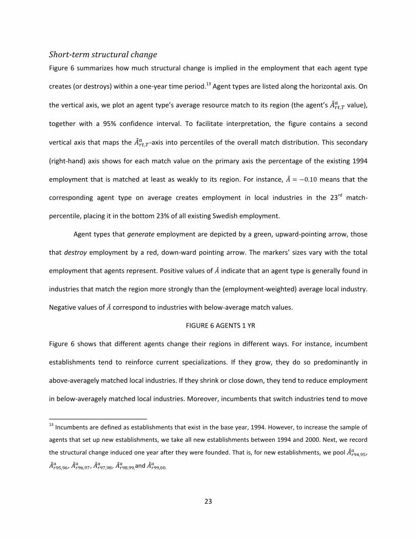
creates (or destroys) within a one-year time period.13 Agent types are listed along the horizontal axis. On
the vertical axis, we plot an agent type’s average resource match to its region (the agent’s �̃�𝑟𝑡,𝑇𝑎 value),
together with a 95% confidence interval. To facilitate interpretation, the figure contains a second
vertical axis that maps the �̃�𝑟𝑡,𝑇𝑎 -axis into percentiles of the overall match distribution. This secondary
(right-hand) axis shows for each match value on the primary axis the percentage of the existing 1994
employment that is matched at least as weakly to its region. For instance, �̃� = −0.10 means that the
corresponding agent type on average creates employment in local industries in the 23rd match-
percentile, placing it in the bottom 23% of all existing Swedish employment.
Agent types that generate employment are depicted by a green, upward-pointing arrow, those
that destroy employment by a red, down-ward pointing arrow. The markers’ sizes vary with the total
employment that agents represent. Positive values of �̃� indicate that an agent type is generally found in
industries that match the region more strongly than the (employment-weighted) average local industry.
Negative values of �̃� correspond to industries with below-average match values.
FIGURE 6 AGENTS 1 YR
Figure 6 shows that different agents change their regions in different ways. For instance, incumbent
establishments tend to reinforce current specializations. If they grow, they do so predominantly in
above-averagely matched local industries. If they shrink or close down, they tend to reduce employment
in below-averagely matched local industries. Moreover, incumbents that switch industries tend to move
13
Incumbents are defined as establishments that exist in the base year, 1994. However, to increase the sample of
agents that set up new establishments, we take all new establishments between 1994 and 2000. Next, we record
the structural change induced one year after they were founded. That is, for new establishments, we pool �̃�𝑟94,95𝑎 ,
�̃�𝑟95,96𝑎 , �̃�𝑟96,97
𝑎 , �̃�𝑟97,98𝑎 , �̃�𝑟98,99,
𝑎 and �̃�𝑟99,00.𝑎

24
to industries that fit the region better: on average, they abandon industries in the 40th and enter
industries in the 47th match-percentile. In contrast, new establishments tend to diversify a region’s
resource base. Indeed, in support of Hypothesis 1 (incumbents induce less structural change than new
establishments), almost all new-establishment types display below-average �̃�-values. However, they do
so to different extents.
New subsidiaries of existing firms occupy on average more strongly matched industries (42nd
match-percentile), than those of entrepreneurs (29th match-percentile). This supports Hypothesis 3b
over Hypothesis 3a: entrepreneurs induce more structural change than expanding firms.
Furthermore, establishments that come from outside the region induce much more structural
change than those that originate from within the region. On average, local entrepreneurs create
employment in the 32nd match-percentile, against the 22nd for non-local entrepreneurs, which is both
statistically and economically significant. The difference between new subsidiaries of local (59th match-
percentile) and non-local (33rd) firms is even larger. We conclude therefore that there is strong support
for Hypothesis 2.
Interestingly, and contradicting hypothesis 1, the new subsidiaries of local firms are mostly
found in industries that are closely related to the region’s industry mix. Just like incumbent
establishments, these subsidiaries reinforce the existing resource base. However, local firms’ new
subsidiaries can be regarded as incumbent growth that is accommodated in new facilities. In hindsight,
it is therefore not surprising to find these establishments to behave much like growing incumbents.14
14
These findings are related to those in Dumais et al. (2002) on changes in industries’ spatial concentration. Consistent with our findings, these authors show that new establishments have a deagglomerating effect on industries. Furthermore, Dumais and colleagues find that exits lead to a strengthening of existing agglomeration patterns, which is similar to our finding that exits reinforce existing capability structures. However, whereas Dumais and co-authors find that the growth and decline patterns of incumbents weaken spatial concentration, we find these patterns to strengthen existing specializations.
25
Overall, we conclude that the new establishments of non-local entrepreneurs change a regional
resource base the most, followed by those of non-local firms.
Long-term structural change
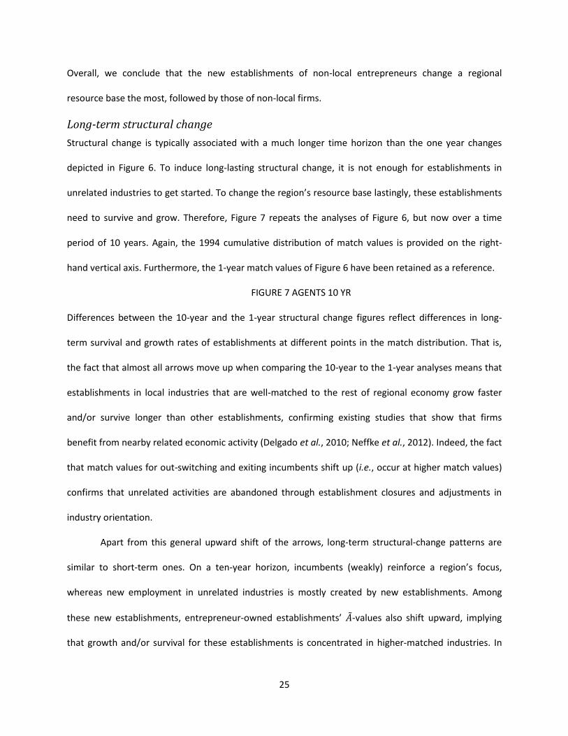
Structural change is typically associated with a much longer time horizon than the one year changes
depicted in Figure 6. To induce long-lasting structural change, it is not enough for establishments in
unrelated industries to get started. To change the region’s resource base lastingly, these establishments
need to survive and grow. Therefore, Figure 7 repeats the analyses of Figure 6, but now over a time
period of 10 years. Again, the 1994 cumulative distribution of match values is provided on the right-
hand vertical axis. Furthermore, the 1-year match values of Figure 6 have been retained as a reference.
FIGURE 7 AGENTS 10 YR
Differences between the 10-year and the 1-year structural change figures reflect differences in long-
term survival and growth rates of establishments at different points in the match distribution. That is,
the fact that almost all arrows move up when comparing the 10-year to the 1-year analyses means that
establishments in local industries that are well-matched to the rest of regional economy grow faster
and/or survive longer than other establishments, confirming existing studies that show that firms
benefit from nearby related economic activity (Delgado et al., 2010; Neffke et al., 2012). Indeed, the fact
that match values for out-switching and exiting incumbents shift up (i.e., occur at higher match values)
confirms that unrelated activities are abandoned through establishment closures and adjustments in
industry orientation.
Apart from this general upward shift of the arrows, long-term structural-change patterns are
similar to short-term ones. On a ten-year horizon, incumbents (weakly) reinforce a region’s focus,
whereas new employment in unrelated industries is mostly created by new establishments. Among
these new establishments, entrepreneur-owned establishments’ �̃�-values also shift upward, implying
that growth and/or survival for these establishments is concentrated in higher-matched industries. In

26
contrast, the new subsidiaries of existing firms either remain at the same match-value (local firms) or
even move down (non-local firms). Apparently, unlike the new establishments of entrepreneurs,
subsidiaries of non-local firms grow more and/or survive longer in low-match industries. As a result,
although confidence intervals partially overlap, new subsidiaries of non-local firms end up in match
values below those of non-local entrepreneurs. In the long run, non-local firms thus surpass
entrepreneurs as the main agents of structural change.
Plant survival
To assess more carefully the differences in survival patterns alluded to above, we investigate for which
agents the presence of related industries is associated with higher establishment survival rates. To do
so, for each new establishment between 1995 and 2000, we create a dummy that is valued at one if it
survives for at least 10 years and at zero otherwise. Next, we estimate linear probability models, i.e., we
regress this dummy variable on a set of founding agent dummies and their interactions with the natural
logarithm of related employment in the region.15 We include entry-year, region and industry dummies
to isolate the effect of the founder type. However, because we are interested in how survival rates differ
by agent type, not necessarily in why they do so, we do not control for any other establishment
characteristics, such as start-up size. Table 5 summarizes the results.
TABLE 5: SURVIVAL
The unconditional average survival rate for new establishments is 0.201. The model in Column (1) of
Table 5 contains only a dummy for whether or not an establishment’s founder comes from outside the
region. The negative coefficient on this dummy shows that establishments of non-local founders have a
2.1 percentage-point lower survival rate than those of local founders. Column (2) adds interactions with
the amount of related employment in the region. Plants that enter regions with a large amount of
15
In these regression analyses, a coefficient for log-transformed employment figures is easier to interpret a coefficient for the match variable, which is normalized against industry and region size. Instead we rely on industry and region fixed effects to absorb any idiosyncrasies at the industry or regional level.

27
related employment tend to survive longer, especially if their founders are local.16 The estimated
coefficients suggest that doubling the related employment translates into a 1.2 percentage-point
increase in survival rates for local establishments and a 0.9 percentage-point increase for non-local
establishments.17 When we split founders into entrepreneurs and existing firms (Columns (3) and (4)),
even larger differences emerge. Whereas firm-owned subsidiaries generally have higher survival rates
than entrepreneur-owned establishments, only the entrepreneur-owned establishments seem sensitive
to the amount of related employment in the region. Column (5) further subdivides establishments by
their geographical origin. Regardless of whether an establishment was founded by local or non-local
entrepreneurs, survival rates of entrepreneur-owned establishments are always lower than those of
firm subsidiaries. However, whereas local roots are associated with higher survival rates among
entrepreneurs (the omitted category consists of local entrepreneurs), the opposite holds for firm-owned
subsidiaries: here, non-local origins are associated with higher survival rates. Furthermore, Column (6)
again suggests that related employment in the region only matters for entrepreneur-owned, not for
firm-owned establishments.18
These findings are consistent with the theoretical framework of section 2. Firstly, the finding
depicted in Column (4) – that only entrepreneur-owned establishments display significantly higher
survival rates in regions with related employment – is in line with the notion that entrepreneurs depend
more strongly on local resources than subsidiaries of larger firms. Secondly, the hypothesis that
entrepreneurs cannot draw on a parent firm to compensate for outsiders’ lack of access to local
resources explains why, in Column (5), we find higher failure rates for non-local entrepreneurs but not
for non-local firms. However, such a causal interpretation is hazardous, because the decision to enter a
16
A t-test reveals that this difference is statistically significant at a p-value of 0.026. 17
The effect size of raising related employment by a factor 𝜉 is calculated as: point estimate × ln (ξ). 18
Although the effect of ln(rel. emp. ) differs between local and non-local entrepreneurs, this difference is not statistically significant (i.e., the difference of the interaction with ln(rel. emp. ) is statistically insignificant).

28
region is endogenous, even conditional on industry and region fixed effects. For instance, the fact that
firm-owned subsidiaries seem unaffected by the local amount of related employment could alternatively
mean that they are more careful when choosing a location. In that case, the absence of an association
with higher survival rates is due to the fact that firms make fewer mistakes (or take less risk) when
deciding where to locate, not because they draw fewer benefits from the local environment.
Aggregate structural change
So far, we have determined the main agents of regional structural change in terms of the intensity, not
the amount of structural change they induce. However, some agent types are more prevalent than
others. For instance, entrepreneurs set up far more establishments than existing firms do: the new
establishments of local entrepreneurs outnumber those of non-local entrepreneurs 5-to-1 and those of
non-local firms 20-to-1. Therefore, although the intensity with which they shift a region’s resource base
is lower, as a group, local entrepreneurs may still constitute an important factor in this shift. To
determine the structural change that agents produce at the group level, we look at the employment
new establishments create on a ten-year horizon in the bottom 5th and bottom 10th match percentiles.
This employment is least related to the rest of the local economy and therefore represents most radical
structural change. Non-local firms contribute about 23% of all new-establishment employment, and they
account for 27% (24%) of this employment in the bottom 5th (10th) percentile. More strikingly, although
non-local entrepreneurs create just 9% of overall new-establishment employment, they produce 29%
(23%) of new-establishment employment at the bottom of the match distribution. Taken together, new
establishments with non-local origins create 56% (47%) in these bottom percentiles, even though they
represent just a third of all new-establishment employment, once more showing the importance of non-
local agents in the process of regional structural change.
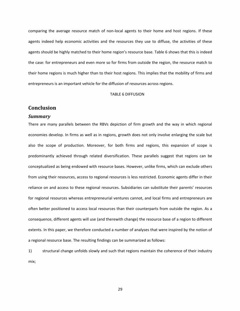
Spatial diffusion through the mobility of firms and entrepreneurs
The finding that non-local agents renew the resource base of a region suggests that non-local agents are
important in the diffusion of industries and the resources they require. We explore this further by
29
comparing the average resource match of non-local agents to their home and host regions. If these
agents indeed help economic activities and the resources they use to diffuse, the activities of these
agents should be highly matched to their home region’s resource base. Table 6 shows that this is indeed
the case: for entrepreneurs and even more so for firms from outside the region, the resource match to
their home regions is much higher than to their host regions. This implies that the mobility of firms and
entrepreneurs is an important vehicle for the diffusion of resources across regions.
TABLE 6 DIFFUSION
Conclusion
Summary
There are many parallels between the RBVs depiction of firm growth and the way in which regional
economies develop. In firms as well as in regions, growth does not only involve enlarging the scale but
also the scope of production. Moreover, for both firms and regions, this expansion of scope is
predominantly achieved through related diversification. These parallels suggest that regions can be
conceptualized as being endowed with resource bases. However, unlike firms, which can exclude others
from using their resources, access to regional resources is less restricted. Economic agents differ in their
reliance on and access to these regional resources. Subsidiaries can substitute their parents’ resources
for regional resources whereas entrepreneurial ventures cannot, and local firms and entrepreneurs are
often better positioned to access local resources than their counterparts from outside the region. As a
consequence, different agents will use (and therewith change) the resource base of a region to different
extents. In this paper, we therefore conducted a number of analyses that were inspired by the notion of
a regional resource base. The resulting findings can be summarized as follows:
1) structural change unfolds slowly and such that regions maintain the coherence of their industry
mix;

30
2) existing establishments tend to deepen a region’s resource base by destroying employment in
unrelated industries and creating employment in related ones, whereas most new establishments create
employment in unrelated industries, thereby shifting the region’s resource base;
3) entrepreneur-owned establishments induce more structural change in the short run than in the
long run, whereas the reverse holds for new subsidiaries of existing firms;
4) consistent with finding 3), whereas entrepreneur-owned establishments tend to survive longer
in regions with more related employment, no such association is found for firm-owned subsidiaries;
5) moreover, being local is associated with higher survival rates for entrepreneurs, whereas the
opposite holds for firm-owned subsidiaries;
6) non-local agents induce significantly more structural change than agents from within the region;
7) and non-local agents diffuse activities from their home regions, in which these activities are
typically much better matched to local resources in their home region, as compared to local resources in
their new host regions.
These findings do not depend on the use of skill relatedness to measure related employment, as
these findings are replicated using alternative relatedness indices based on the industry classification
system and on input-output linkages in Appendix D.
Discussion
We have differentiated the industries mix a region currently hosts from the resources that allow these
industries to thrive. This distinction is in itself important for local policy-making, but also for firms and
entrepreneurs who need to choose suitable locations for their activities. Indeed, our finding that,
although the industry mixes of regions fluctuate strongly, their resource bases change much more
slowly, highlights that the current constellation of industries in a region is just one manifestation of how
the local resources can be put to work. This suggests understanding a region’s strength and weaknesses
at the deeper level of its resources, shifting the focus from the industries that are present in the region
31
to those that could be present. Moreover, the indices we proposed can be used to quantify these
strengths and weaknesses in terms of industries’ resource match to regional economies.
Our application of this framework to identify the agents of structural change in a region provides
important lessons for regional renewal, a topic that ranks highly on the agenda of local policy makers. In
the American context, cities like Detroit and Pittsburg are prime examples of urban economies that at
some point ran into the limits of their economic specializations in car manufacturing and steel making
respectively. In Europe, regional renewal and transformation are important goals of the European
Union’s (EU) smart specialization agenda.19 Such policy frameworks typically place high expectations on
entrepreneurs to discover new activities that are feasible in a region (Hausmann and Rodrik, 2003; Foray
and Goenaga, 2013; McCann and Ortega-Argilés, 2013). However, our results question the canonical
image of the heroic Schumpeterean entrepreneur as the prime transformative force in local economies.
Although entrepreneurs do bring change to a region, they often fail to do so sustainably. Indeed, a more
important factor in structural change than Silicon Valley-style homegrown entrepreneurship seems to
be mobility: unrelated activities are typically transferred from elsewhere by entrepreneurs and firms
from outside the region.
Although entrepreneurs who play a key role in shaking up the regional status quo undoubtedly
exist, we find them to be rather exceptional. Indeed, entrepreneurial ventures much more often fail in
the absence of related economic activities than new subsidiaries of existing firms. We attributed this to
the fact that, whereas subsidiaries have direct, intra-firm links tying them to relevant resources in their
region of origin, non-local entrepreneurs must rely on much weaker, social ties to their home region.
Indeed, this reasoning is supported by the finding in Frost (2001) that foreign subsidiaries draw
19
In a recent policy report for the European Commission, Foray and Goenaga (2013, p. 1) argue that “[smart specialization] seeks robust and transparent means for nominating those new activities, at regional level, that aim at exploring and discovering new technological and market opportunities and at opening thereby new domains for constructing regional competitive advantages.”
32
substantially on their home country’s knowledge base. Moreover, subsidiaries can tap the resource pool
of their parents, which helps them to overcome the liability of newness that activities face in regions
with few related activities. For entrepreneurs, our findings suggest that, absent the ties to a parent
firm’s resources, it is hard to take activities to places where they are badly matched to the existing local
economy. For policy makers, they mean that transformation policies that rely wholly on local
entrepreneurial discovery processes are not without risks.
Caveats
There are a number of caveats in to be considered. First, we only investigate the sources of structural
change, not whether structural change is desirable or not. Most probably, leveraging existing resources
will be attractive in the short run but, in the long run, regions will have to adapt to new economic
realities. However, long-run structural change can be accomplished through a series of small steps, in a
process of related diversification that gradually moves the region away from its traditional resource
base. The optimal balance of related and unrelated diversification – and hence, the optimal speed of
structural change – is an important topic, but left for future research.
Second, by focusing on the new establishments that enter an economy, we have mostly
highlighted the diversification aspect of structural change. However, although our analyses show that
incumbent exit and decline typically take place in unrelated industries, there are well-known examples
in which the core industries of a region collapse (e.g., Grabher, 1993). In these cases, structural change
occurs because of the loss of a core industry and a concurrent erosion of local resources.
Third, our analyses answer the question of who introduces unrelated economic activities in a
region. In essence, this question is descriptive, not causal. We therefore remain agnostic about whether
the reported differences among agent types reflect different intrinsic capacities for structural change or,
for instance, differences in location choices. Similarly, in the survival analyses, we cannot distinguish
33
spatial sorting of establishments from agglomeration externalities, an issue that has attracted
considerable attention in urban economics (e.g., Combes et al., 2008).
Future research
Finally, our study raises a number of new questions. Firstly, the finding that new subsidiaries of existing
firms are better able to grow and survive in unrelated environments than stand-alone establishments
begs the question of why this is the case. Our proposal – that firm-owned establishments draw on their
parent firms’ resources – remains to be proven, and related questions arise of how and across what
distance multi-establishment firms can accomplish this. Secondly, the fact that firms switch industry
affiliations from low-match to high-match industries suggests that firm strategies interact with
regionally available resources in ways that are still poorly understood. We hope that the framework we
developed here will prove useful in approaching these and other questions on how regional economies
and their resource bases co-evolve with the firms they host.
34
REFERENCES
Alcácer J, Chung W. 2007. Location strategies and knowledge spillovers. Management Science 54(5): 760-776.
Alcácer J, Chung W. 2013. Location strategies for agglomeration economies. Management Science. Almeida P, Kogut B (1999) Localization of knowledge and the mobility of engineers. Management Science
45(7): 905–917 Andersson J, Arvidson G. 2006. Företagens och arbetsställenas dynamik (FAD). Memo, Statistics Sweden. Barney J. 1991. Firm resources and sustained competitive advantage. Journal of Management 17: 99–120. Bathelt H, Malmberg A, Maskell P. 2004. Clusters and knowledge: local buzz, global pipelines and the
process of knowledge creation. Progress in Human Geography 28: 31-56. Boschma RA. 2004. Competitiveness of regions from an evolutionary perspective, Regional Studies 38(9):
1001-1014. Boschma R, Frenken K. 2011. Technological relatedness and regional branching, in: H. Bathelt, M.P.
Feldman and D.F. Kogler (eds.), Beyond Territory. Dynamic Geographies of Knowledge Creation, Diffusion and Innovation, Routledge, London and New York, pp. 64-81.
Boschma RA, Minondo A, Navarro M. 2013. The Emergence of New Industries at the Regional Level in Spain: A Proximity Approach Based on Product Relatedness. Economic Geography 89(1): 29-51.
Bryce DJ, Winter SG. 2009. A general inter-industry relatedness index. Management Science 55: 1570-1585.
Combes P-Ph, Duranton D, Gobillon L. 2008. Spatial wage disparities: Sorting matters! Journal of Urban Economics 63(2): 723-742.
Cooke P.H., Morgan K. (1998). The Associational Economy. Firms, Regions, and Innovation. Oxford: Oxford University Press.
Cramer JS, Hartog J, Jonker N, Van Praag CM. 2002. Low risk aversion encourages the choice for entrepreneurship: an empirical test of a truism. Journal of Economic Behavior & Organization 48(1): 29–36.
Dahl MS, Sorenson O. 2012. Home sweet home: Entrepreneurs' location choices and the performance of their ventures, Management Science 58(6): 1059–1071.
Dauth, W. 2010. The mysteries of the trade: employment effects of urban interindustry spillovers. IAB Discussion Paper 15/2010: 1-25.
Delgado M, Porter ME, Stern S. 2010. Clusters and entrepreneurship. Journal of Economic Geography 10(4): 495-518.
Delgado M, Porter ME, Stern S. 2013. Defining clusters of related industries, HBS working paper. Dumais G, Ellison G, Glaeser EL. 2002. Geographic concentration as a dynamic process. Review of
Economics and Statistics, 84(2): 193-204. Duranton G, Puga D. 2004. Micro-foundation of urban agglomeration economies, in Henderson J, Thisse
JF. (Eds) Handbook of Urban and Regional Economics, vol 4, pp. 2065-2118. Elsevier, Amsterdam. Eisenhardt KM, Martin JA. 2000. Dynamic capabilities: What are they? Strategic Management Journal 21:
1105–1121. Ellison G, Glaeser EL, Kerr WR. 2010. What Causes Industry Agglomeration? Evidence from
Coagglomeration Patterns. American Economic Review, 100(3): 1195–1213. Essletzbichler J. 2013. Relatedness, Industrial Branching and Technological Cohesion in US Metropolitan
Areas. Regional Studies, 10.1080/00343404.2013.806793 Faggian A. McCann Ph. (2006). Human capital flows and regional knowledge assets: a simultaneous
equation approach. Oxford Economic Papers 52: 475–500. Farjoun M. 1994. Beyond industry boundaries: Human expertise, diversification and resource-related
industry groups. Organization Science 5(2): 185–199.

35
Florida R, Mellander C, Stolarick K. 2012. Geographies of scope: an empirical analysis of entertainment, 1970–2000. Journal of Economic Geography, 12(1): 183-204.
Foray D, Goenaga X. 2013. The goals of smart specialisation, JRC Scientific and Policy Report, S3 Policy Brief Series No. 01/2013.
Frenken K, Boschma RA. 2007. A theoretical framework for economic geography: industrial dynamics and urban growth as a branching process. Journal of Economic Geography 7 (5), pp. 635-649.
Frost TS. 2001. The geographic sources of foreign subsidiaries' innovations, Strategic Management Journal 22(2): 101-123.
Gertler, M.S. 2003. Tacit knowledge and the economic geography of context, or the undefinable tacitness of being (there), Journal of Economic Geography, 3: 75-99.
Ghemawat P. 1986. Sustainable advantage, Harvard Business Review, 64(5): 53–58. Giuliani E. 2007. The selective nature of knowledge networks in clusters: evidence from the wine industry,
Journal of Economic Geography 7: 139-168. Glaeser EL. 2005. Reinventing Boston: 1630–2003, Journal of Economic Geography 5(2): 119-153. Glaeser EL, Kerr WR. 2009. Local Industrial Conditions and Entrepreneurship: How Much of the Spatial
Distribution Can We Explain? Journal of Economics & Management Strategy 18(3): 623-663. Glaeser, E.L., Kallal, H.D., Scheinkman, J.A., Schleifer A. (1992) Growth in Cities, Journal of Political
Economy, 100 (6): 1126-1152. Glaeser EL, Kerr WR, Ponzetto GAM. 2010. Clusters of entrepreneurship, Journal of Urban Economics
67(1):150–168. Grabher G. (1993) The weakness of strong ties: the lock-in of regional development in the Ruhr area, in
Grabher G. (ed.) The Embedded Firm. London: Routledge. Grant RM. 1996. Toward a knowledge-based theory of the firm. Strategic Management Journal 17: 109–
122. Grant RM, Spender JC. 1996. Knowledge and the firm: overview. Strategic Management Journal 17: 5–9. Hausmann R, Rodrik D. 2003. Journal of Development Economics 72(2): 603-633. Helfat CE, Peteraf MA. 2003. The dynamic resource-based view: capability lifecycles, Strategic
Management Journal, 24(10): 997–1010. Henderson, J.V., Kuncoro, A., Turner, M. (1995) Industrial development in cities, Journal of Political
Economy, 103:1067-1085. Henderson R, Cockburn I. 1994. Measuring Competence? Exploring Firm Effects in Pharmaceutical
Research, Strategic Management Journal 15: 63–84. Hidalgo CA, Klinger B, Barabási A-L, Hausmann R. 2007. The Product Space Conditions the Development of
Nations. Science 317: 482-487. Jacobs J. 1969. The Economy of Cities. New York: Vintage Books. Lawson C. 1999. Towards a competence theory of the region, Cambridge Journal of Economics 23(2): 151-
166. Lawson C, Lorenz E. 1999. Collective learning, tacit knowledge and regional innovative capacity, Regional
Studies 33: 305-317. Maskell P. 2005. Towards a Knowledge-Based Theory of the Geographical Cluster. In: Breschi S, Malerba F
(Eds.). Clusters, Networks, and Innovation. Oxford: Oxford University Press. Chapter 15: 411-432. Maskell P, Malmberg A. 1999. Localised learning and industrial competitiveness, Cambridge Journal of
Economics 23(2): 167-185. McCann Ph, Ortega-Argilés R. 2013. Smart specialization, regional growth and applications to European
Union cohesion policy, Regional Studies, in press. McCann Ph, Simonen J. 2005. Innovation, knowledge spillovers and local labour markets. Papers in
Regional Science 84(3): 465-485.
36
Montgomery CA, Wernerfelt B. 1988. Diversification, Ricardian Rents, and Tobin's q, RAND Journal of Economics 19(4): 623-632.
Muneepeerakul R, Lobo J, Shutters ST, Goméz-Liévano A, Qubbaj MR. 2013. Urban Economies and Occupation Space: Can They Get “There” from “Here”? PLoS ONE 8(9): e73676.
Neffke FMH, Henning M. 2013. Skill relatedness and firm diversification. Strategic Management Journal. 34(3): 297-316.
Neffke FMH, Henning M, Boschma RA. 2012. The impact of aging and technological relatedness on agglomeration externalities: a survival analysis. Journal of Economic Geography 12(2): 485-517.
Neffke FMH, Henning M, Boschma RA. 2011. How do regions diversify over time? Industry relatedness and the development of new growth paths in regions. Economic Geography 87: 237-265.
Neffke FMH, Hidalgo C, Otto A, Weyh A. 2013. Inter-industry labor flows. mimeo. Palich LE, Cardinal LB, Miller C. 2000. Curvilinearity in the diversification-performance linkage: An
examination of over three decades of research. Strategic Management Journal 21: 155–174. Pendall R, Foster KA, Cowell M. 2010. Resilience and regions: building understanding of the metaphor,
Cambridge Journal of Regions, Economy and Society: 3, 71–84 Penrose ET. 1959. The Theory of the Growth of the Firm. Blackwell: Oxford, UK. Peteraf MA. 1993. The cornerstones of competitive advantage: A resource-based view. Strategic
Management Journal 14: 179–191. Porter ME. 1987. From competitive advantage to corporate strategy. Harvard Business Review 65(3): 43–
59. Porter ME. 1990. The Competitive Advantage of Nations. Macmillan, London. Porter, M.E. (1998). Clusters and the new economics of competition. Harvard Business Review 76
(November-December): 77-90. Porter M. 2003. The Economic Performance of Regions. Regional Studies 37(6-7): 549–578. Pouder R, St. John CH. 1996. Hot Spots and Blind Spots: Geographical Clusters of Firms and Innovation,
Academy of Management Review 21(4): 1192-1225. Rosenthal SS, Strange WC. 2004. Evidence on the Nature and Sources of Agglomeration Economies. In:
Handbook of Urban and Regional Economics (4). Henderson J., Thisse J.-F. (eds.). Amsterdam: Elsevier. SCB. 2011. Longitudinell integrationsdatabas för sjukförsäkrings- och arbetsmarknadsstudier (LISA) 1990-
2009. Arbetsmarknads- och utbildningsstatistik 2011:4. Statistiska centralbyrån/Statistics Sweden. Schumpeter JA. 1934. The theory of economic development. Cambridge: Harvard University Press. Sorenson O, Audia PG. 2000. The social structure of entrepreneurial activity: Geographic concentration of
footwear production in the United States, 1940–1989, American Journal of Sociology 106(2): 424-462. Storper M. 1995. The resurgence of regional economies, ten years later: The region as a nexus of
untraded interdependencies, European Urban and Regional Studies 2: 191-221. Storper M, Venables T. 2004. Buzz: face-to-face contact and the urban economy Journal of Economic
Geography, 4 (4). 351-370. Teece DJ. 1982. Towards an economic theory of the multiproduct firm. Journal of Economic Behavior and
Organization 3: 39–63. Teece DJ, Pisano G, Shuen A. 1997. Dynamic capabilities and strategic management. Strategic
Management Journal 18: 509–533. Teece DJ, Rumelt R, Dosi G, Winter S. 1994. Understanding corporate coherence. Theory and evidence.
Journal of Economic Behavior and Organization 23: 1-30. Tushman ML, Anderson Ph. 1986. Technological discontinuities and organizational environments,
Administrative Science Quarterly 31(3): 439-465. Wernerfelt B. 1984. A resource-based view of the firm. Strategic Management Journal 5: 171–180. Zhao H, Seibert SE. 2006. The Big Five personality dimensions and entrepreneurial status: A meta-
analytical review. Journal of Applied Psychology, 91(2): 259-271.

37
Tables and figures
Table 1: Diversity, industrial change, coherence and structural change
Static Dynamic
Industries Diversity
Measured by: entropy
Underlying question: How many different
industries are there and how equal is their
size distribution?
Industrial change
Measured by: cosine distance
Underlying question: How fast are new
industries introduced and how much does
the size distribution of activities change?
Resources Coherence
Measured by: see Table 2
Underlying question: How similar are the
resources required by the various industries
in the region? That is, how related are the
industries in a region to one another?
Structural change
Measured by: see Table 2
Underlying question: To what extent does
the resources base change due to changes
in the region’s industries? That is, how
related are current industries to the
industry mix in the base year?
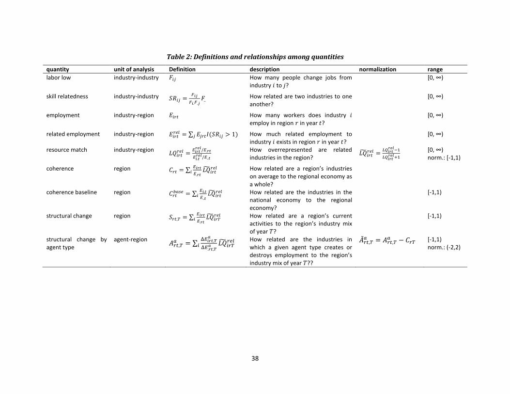
38
Table 2: Definitions and relationships among quantities
quantity unit of analysis Definition description normalization range
labor low industry-industry 𝐹𝑖𝑗 How many people change jobs from industry 𝑖 to 𝑗?
[0, ∞)
skill relatedness industry-industry 𝑆𝑅𝑖𝑗 =𝐹𝑖𝑗
𝐹𝑖.𝐹.𝑗𝐹..
How related are two industries to one another?
[0, ∞)
employment industry-region 𝐸𝑖𝑟𝑡 How many workers does industry 𝑖 employ in region 𝑟 in year 𝑡?
[0, ∞)
related employment industry-region 𝐸𝑖𝑟𝑡𝑟𝑒𝑙 = ∑ 𝐸𝑗𝑟𝑡𝐼(𝑆𝑅𝑖𝑗 > 1)𝑗 How much related employment to
industry 𝑖 exists in region 𝑟 in year 𝑡? [0, ∞)
resource match industry-region
𝐿𝑄𝑖𝑟𝑡𝑟𝑒𝑙 =
𝐸𝑖𝑟𝑡𝑟𝑒𝑙/𝐸.𝑟𝑡
𝐸𝑖.𝑡𝑟𝑒𝑙/𝐸..𝑡
How overrepresented are related industries in the region?
𝐿�̃�𝑖𝑟𝑡𝑟𝑒𝑙 =
𝐿𝑄𝑖𝑟𝑡𝑟𝑒𝑙−1
𝐿𝑄𝑖𝑟𝑡𝑟𝑒𝑙+1
[0, ∞) norm.: [-1,1)
coherence region 𝐶𝑟𝑡 = ∑𝐸𝑖𝑟𝑡
𝐸.𝑟𝑡𝐿�̃�𝑖𝑟𝑡
𝑟𝑒𝑙𝑖 How related are a region’s industries
on average to the regional economy as a whole?
coherence baseline region 𝐶𝑟𝑡𝑏𝑎𝑠𝑒 = ∑
𝐸𝑖.𝑡
𝐸..𝑡𝑖 𝐿�̃�𝑖𝑟𝑡
𝑟𝑒𝑙 How related are the industries in the national economy to the regional economy?
[-1,1)
structural change region 𝑆𝑟𝑡,𝑇 = ∑𝐸𝑖𝑟𝑡
𝐸.𝑟𝑡𝑖 𝐿�̃�𝑖𝑟𝑇
𝑟𝑒𝑙 How related are a region’s current activities to the region’s industry mix of year 𝑇?
[-1,1)
structural change by agent type
agent-region 𝐴𝑟𝑡,𝑇
𝑎 = ∑Δ𝐸𝑖𝑟𝑡,𝑇
𝑎
Δ𝐸.𝑟𝑡,𝑇𝑎 𝐿�̃�𝑖𝑟𝑇
𝑟𝑒𝑙𝑖
How related are the industries in which a given agent type creates or destroys employment to the region’s industry mix of year 𝑇??
�̃�𝑟𝑡,𝑇𝑎 = 𝐴𝑟𝑡,𝑇
𝑎 − 𝐶𝑟𝑇 [-1,1) norm.: (-2,2)
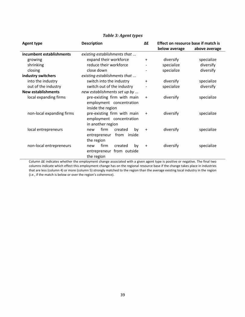
39
Table 3: Agent types
Agent type Description ΔE Effect on resource base if match is below average above average
incumbent establishments existing establishments that ... growing expand their workforce + diversify specialize shrinking reduce their workforce - specialize diversify closing close down - specialize diversify industry switchers existing establishments that ... into the industry switch into the industry + diversify specialize out of the industry switch out of the industry - specialize diversify New establishments new establishments set up by ... local expanding firms pre-existing firm with main
employment concentration inside the region
+ diversify specialize
non-local expanding firms pre-existing firm with main employment concentration in another region
+ diversify specialize
local entrepreneurs new firm created by entrepreneur from inside the region
+ diversify specialize
non-local entrepreneurs new firm created by entrepreneur from outside the region
+ diversify specialize
Column ΔE indicates whether the employment change associated with a given agent type is positive or negative. The final two columns indicate which effect this employment change has on the regional resource base if the change takes place in industries that are less (column 4) or more (column 5) strongly matched to the region than the average existing local industry in the region (i.e., if the match is below or over the region’s coherence).
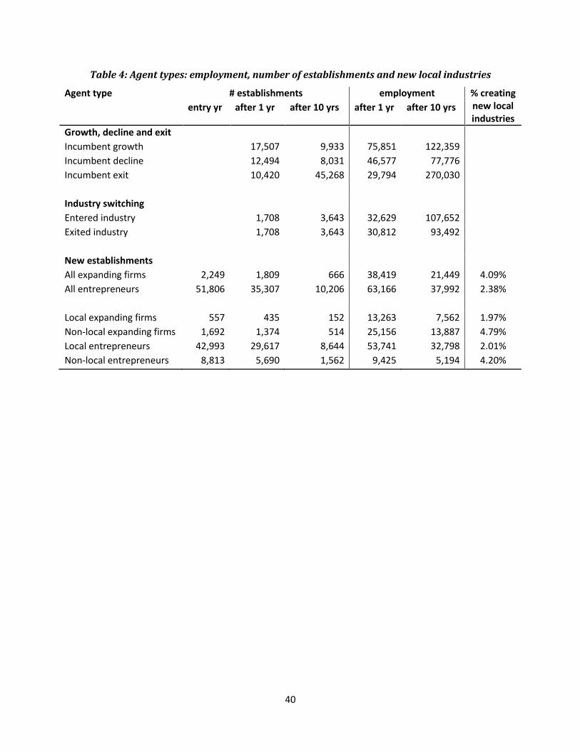
40
Table 4: Agent types: employment, number of establishments and new local industries
Agent type # establishments employment % creating new local industries
entry yr after 1 yr after 10 yrs after 1 yr after 10 yrs
Growth, decline and exit
Incumbent growth 17,507 9,933 75,851 122,359
Incumbent decline 12,494 8,031 46,577 77,776
Incumbent exit 10,420 45,268 29,794 270,030
Industry switching
Entered industry 1,708 3,643 32,629 107,652
Exited industry 1,708 3,643 30,812 93,492
New establishments
All expanding firms 2,249 1,809 666 38,419 21,449 4.09%
All entrepreneurs 51,806 35,307 10,206 63,166 37,992 2.38%
Local expanding firms 557 435 152 13,263 7,562 1.97%
Non-local expanding firms 1,692 1,374 514 25,156 13,887 4.79%
Local entrepreneurs 42,993 29,617 8,644 53,741 32,798 2.01%
Non-local entrepreneurs 8,813 5,690 1,562 9,425 5,194 4.20%
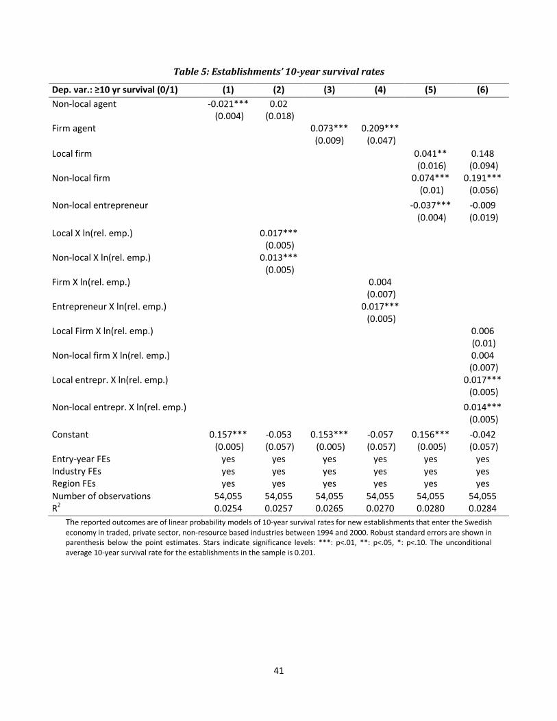
41
Table 5: Establishments’ 10-year survival rates
Dep. var.: ≥10 yr survival (0/1) (1) (2) (3) (4) (5) (6)
Non-local agent -0.021*** (0.004)
0.02 (0.018)
Firm agent 0.073*** (0.009)
0.209*** (0.047)
Local firm 0.041** (0.016)
0.148 (0.094)
Non-local firm 0.074*** (0.01)
0.191*** (0.056)
Non-local entrepreneur -0.037*** (0.004)
-0.009 (0.019)
Local X ln(rel. emp.) 0.017*** (0.005)
Non-local X ln(rel. emp.) 0.013*** (0.005)
Firm X ln(rel. emp.) 0.004 (0.007)
Entrepreneur X ln(rel. emp.) 0.017*** (0.005)
Local Firm X ln(rel. emp.) 0.006 (0.01)
Non-local firm X ln(rel. emp.) 0.004 (0.007)
Local entrepr. X ln(rel. emp.) 0.017*** (0.005)
Non-local entrepr. X ln(rel. emp.) 0.014*** (0.005)
Constant 0.157*** (0.005)
-0.053 (0.057)
0.153*** (0.005)
-0.057 (0.057)
0.156*** (0.005)
-0.042 (0.057)
Entry-year FEs yes yes yes yes yes yes Industry FEs yes yes yes yes yes yes Region FEs yes yes yes yes yes yes
Number of observations 54,055 54,055 54,055 54,055 54,055 54,055 R2 0.0254 0.0257 0.0265 0.0270 0.0280 0.0284
The reported outcomes are of linear probability models of 10-year survival rates for new establishments that enter the Swedish
economy in traded, private sector, non-resource based industries between 1994 and 2000. Robust standard errors are shown in parenthesis below the point estimates. Stars indicate significance levels: ***: p<.01, **: p<.05, *: p<.10. The unconditional average 10-year survival rate for the establishments in the sample is 0.201.
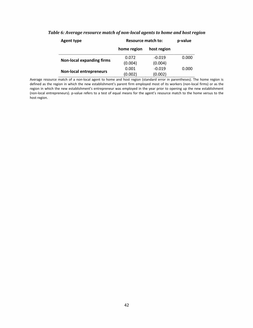
42
Table 6: Average resource match of non-local agents to home and host region
Agent type Resource match to: p-value
home region host region
Non-local expanding firms 0.072
(0.004) -0.019 (0.004)
0.000
Non-local entrepreneurs 0.001
(0.002) -0.019 (0.002)
0.000
Average resource match of a non-local agent to home and host region (standard error in parentheses). The home region is defined as the region in which the new establishment’s parent firm employed most of its workers (non-local firms) or as the region in which the new establishment’s entrepreneur was employed in the year prior to opening up the new establishment (non-local entrepreneurs). p-value refers to a test of equal means for the agent’s resource match to the home versus to the host region.
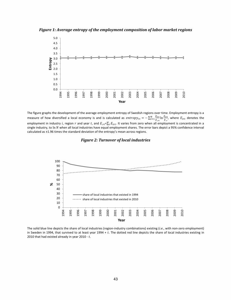
43
Figure 1: Average entropy of the employment composition of labor market regions
The figure graphs the development of the average employment entropy of Swedish regions over time. Employment entropy is a
measure of how diversified a local economy is and is calculated as 𝑒𝑛𝑡𝑟𝑜𝑝𝑦𝑟𝑡 = − ∑𝐸𝑖𝑟𝑡
𝐸..𝑟𝑡ln
𝐸𝑖𝑟𝑡
𝐸..𝑟
𝑁𝑖=1 , where 𝐸𝑖𝑟𝑡 denotes the
employment in industry 𝑖, region 𝑟 and year 𝑡, and 𝐸.𝑟𝑡=∑ 𝐸𝑖𝑟𝑡𝑖 . It varies from zero when all employment is concentrated in a single industry, to ln 𝑁 when all local industries have equal employment shares. The error bars depict a 95% confidence interval calculated as ±1.96 times the standard deviation of the entropy’s mean across regions.
Figure 2: Turnover of local industries
The solid blue line depicts the share of local industries (region-industry combinations) existing (i.e., with non-zero employment) in Sweden in 1994, that survived to at least year 1994 + 𝑡. The dotted red line depicts the share of local industries existing in 2010 that had existed already in year 2010 - 𝑡.
0.0
0.5
1.0
1.5
2.0
2.5
3.0
3.5
4.0
4.5
5.0
19
94
19
95
19
96
19
97
19
98
19
99
20
00
20
01
20
02
20
03
20
04
20
05
20
06
20
07
20
08
20
09
20
10
Entr
op
y
Year
0
10
20
30
40
50
60
70
80
90
100
19
94
19
95
19
96
19
97
19
98
19
99
20
00
20
01
20
02
20
03
20
04
20
05
20
06
20
07
20
08
20
09
20
10
%
Year
share of local industries that existed in 1994
share of local industries that existed in 2010
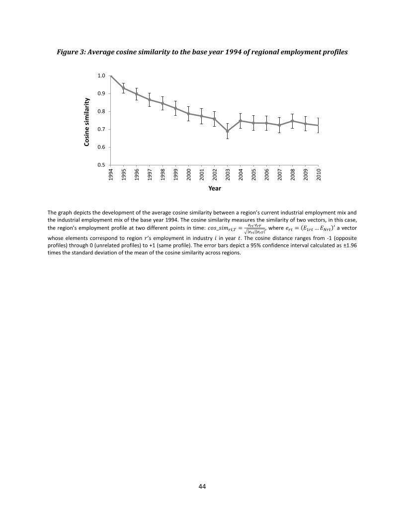
44
Figure 3: Average cosine similarity to the base year 1994 of regional employment profiles
The graph depicts the development of the average cosine similarity between a region’s current industrial employment mix and the industrial employment mix of the base year 1994. The cosine similarity measures the similarity of two vectors, in this case,
the region’s employment profile at two different points in time: 𝑐𝑜𝑠_𝑠𝑖𝑚𝑟𝑡,𝑇 =𝑒𝑟𝑡∙𝑒𝑟𝑇
√|𝑒𝑟𝑡||𝑒𝑟𝑇|, where 𝑒𝑟𝑡 = (𝐸1𝑟𝑡 … 𝐸𝑁𝑟𝑡)′ a vector
whose elements correspond to region 𝑟’s employment in industry 𝑖 in year 𝑡. The cosine distance ranges from -1 (opposite profiles) through 0 (unrelated profiles) to +1 (same profile). The error bars depict a 95% confidence interval calculated as ±1.96 times the standard deviation of the mean of the cosine similarity across regions.
0.5
0.6
0.7
0.8
0.9
1.0
19
94
19
95
19
96
19
97
19
98
19
99
20
00
20
01
20
02
20
03
20
04
20
05
20
06
20
07
20
08
20
09
20
10
Co
sin
e s
imila
rity
Year
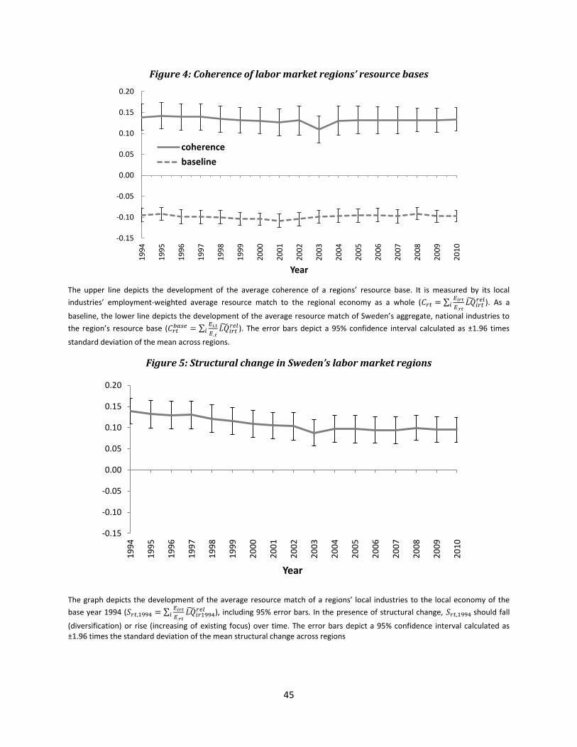
45
Figure 4: Coherence of labor market regions’ resource bases
The upper line depicts the development of the average coherence of a regions’ resource base. It is measured by its local
industries’ employment-weighted average resource match to the regional economy as a whole (𝐶𝑟𝑡 = ∑𝐸𝑖𝑟𝑡
𝐸.𝑟𝑡𝐿�̃�𝑖𝑟𝑡
𝑟𝑒𝑙𝑖 ). As a
baseline, the lower line depicts the development of the average resource match of Sweden’s aggregate, national industries to
the region’s resource base (𝐶𝑟𝑡𝑏𝑎𝑠𝑒 = ∑
𝐸𝑖.𝑡
𝐸..𝑡𝑖 𝐿�̃�𝑖𝑟𝑡
𝑟𝑒𝑙). The error bars depict a 95% confidence interval calculated as ±1.96 times
standard deviation of the mean across regions.
Figure 5: Structural change in Sweden’s labor market regions
The graph depicts the development of the average resource match of a regions’ local industries to the local economy of the
base year 1994 (𝑆𝑟𝑡,1994 = ∑𝐸𝑖𝑟𝑡
𝐸.𝑟𝑡𝑖 𝐿�̃�𝑖𝑟1994
𝑟𝑒𝑙 ), including 95% error bars. In the presence of structural change, 𝑆𝑟𝑡,1994 should fall
(diversification) or rise (increasing of existing focus) over time. The error bars depict a 95% confidence interval calculated as ±1.96 times the standard deviation of the mean structural change across regions
-0.15
-0.10
-0.05
0.00
0.05
0.10
0.15
0.20
19
94
19
95
19
96
19
97
19
98
19
99
20
00
20
01
20
02
20
03
20
04
20
05
20
06
20
07
20
08
20
09
20
10
Year
coherence
baseline
-0.15
-0.10
-0.05
0.00
0.05
0.10
0.15
0.20
19
94
19
95
19
96
19
97
19
98
19
99
20
00
20
01
20
02
20
03
20
04
20
05
20
06
20
07
20
08
20
09
20
10
Year
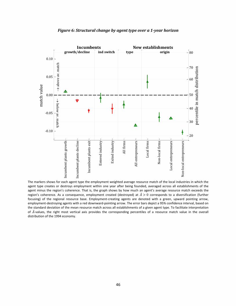
46
Figure 6: Structural change by agent type over a 1-year horizon
The markers shows for each agent type the employment weighted average resource match of the local industries in which the agent type creates or destroys employment within one year after being founded, averaged across all establishments of the agent minus the region’s coherence. That is, the graph shows by how much an agent’s average resource match exceeds the
region’s coherence. As a consequence, employment created (destroyed) at �̃� > 0 corresponds to a diversification (further focusing) of the regional resource base. Employment-creating agents are denoted with a green, upward pointing arrow, employment-destroying agents with a red downward-pointing arrow. The error bars depict a 95% confidence interval, based on the standard deviation of the mean resource match across all establishments of a given agent type. To facilitate interpretation
of �̃�-values, the right most vertical axis provides the corresponding percentiles of a resource match value in the overall distribution of the 1994 economy.
-0.10
-0.05
0.00
0.05
0.10
Incu
mb
ent
pla
nts
gro
wth
Incu
mb
ent
pla
nts
dec
lin
e
Incu
mb
ent
pla
nts
exi
t
En
tere
d i
nd
ust
ry
Exi
ted
in
du
stry
All
fir
ms
All
en
trep
ren
eurs
Lo
cal
firm
s
No
n-l
oca
l fi
rms
Lo
cal
entr
epre
neu
rs
No
n-l
oca
l en
trep
ren
eurs
ma
tch
va
lue
Incumbentsgrowth/decline ind switch
New establishmentstype origin
a
bo
ve
av. m
atch
b
elow
av. m
atch
20
30
40
50
60
70
80
pe
rce
nti
le in
ma
tch
dis
trib
uti
on
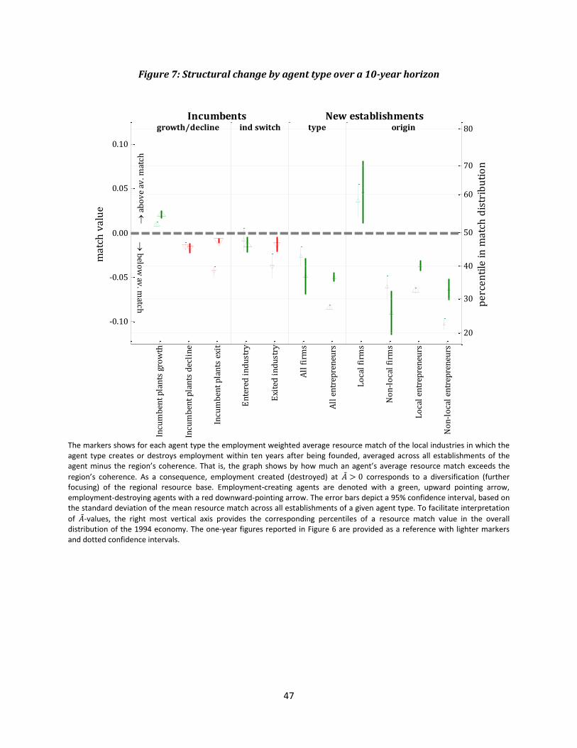
47
Figure 7: Structural change by agent type over a 10-year horizon
The markers shows for each agent type the employment weighted average resource match of the local industries in which the agent type creates or destroys employment within ten years after being founded, averaged across all establishments of the agent minus the region’s coherence. That is, the graph shows by how much an agent’s average resource match exceeds the
region’s coherence. As a consequence, employment created (destroyed) at �̃� > 0 corresponds to a diversification (further focusing) of the regional resource base. Employment-creating agents are denoted with a green, upward pointing arrow, employment-destroying agents with a red downward-pointing arrow. The error bars depict a 95% confidence interval, based on the standard deviation of the mean resource match across all establishments of a given agent type. To facilitate interpretation
of �̃�-values, the right most vertical axis provides the corresponding percentiles of a resource match value in the overall distribution of the 1994 economy. The one-year figures reported in Figure 6 are provided as a reference with lighter markers and dotted confidence intervals.
-0.10
-0.05
0.00
0.05
0.10
Incu
mb
ent
pla
nts
gro
wth
Incu
mb
ent
pla
nts
dec
lin
e
Incu
mb
ent
pla
nts
exi
t
En
tere
d i
nd
ust
ry
Exi
ted
in
du
stry
All
fir
ms
All
en
trep
ren
eurs
Lo
cal
firm
s
No
n-l
oca
l fi
rms
Lo
cal
entr
epre
neu
rs
No
n-l
oca
l en
trep
ren
eurs
ma
tch
va
lue
Incumbentsgrowth/decline ind switch
New establishmentstype origin
a
bo
ve
av. m
atch
b
elow
av. m
atch
20
30
40
50
60
70
80
pe
rce
nti
le in
ma
tch
dis
trib
uti
on

48
Appendix A: Classification of industries
Table A1: Industries included in the analyses
Industry codes Description Definition industry Included
0000 - 1499 Agriculture, hunting and forestry + Fishing + Mining and quarrying
Traded, resource-based no
1500 - 3999 Manufacturing Traded, not resource-based yes
4000 - 4999 Electricity, gas and water supply + Construction
Non-traded no
5000 - 5199 Wholesale and retail trade, repair of motor vehicles, motorcycles and personal and household goods
Non-traded no
5200 - 5299 Retail trade, except of motor vehicles and motorcycles; repair of personal and household goods
Non-traded no
5500 - 5599 Hotels and restaurants Non-traded no
6000 - 6420 Transport, storage and communication Non-traded no
6500 - 6999 Financial intermediation, except insurance and pension funding
Traded, not resource-based yes
7000 - 7199 Real estate + Renting activities Non-traded no
7200 - 7399 Computer and related activities + Research and development
Traded, not resource-based yes
7400 - 7499 Other business activities Traded, not resource-based yes
7500 - 7599 Public administration and defense, compulsory social security
public sector no
7600 - 8599 Education, Health and social work public sector no
8600 - 9999 Other community, social and personal service activities + Activities of households + Extra-territorial organizations and bodies
public sector no
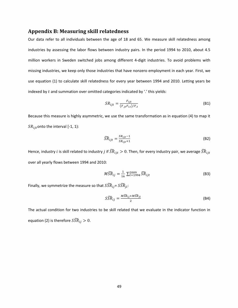
49
Appendix B: Measuring skill relatedness
Our data refer to all individuals between the age of 18 and 65. We measure skill relatedness among
industries by assessing the labor flows between industry pairs. In the period 1994 to 2010, about 4.5
million workers in Sweden switched jobs among different 4-digit industries. To avoid problems with
missing industries, we keep only those industries that have nonzero employment in each year. First, we
use equation (1) to calculate skill relatedness for every year between 1994 and 2010. Letting years be
indexed by 𝑡 and summation over omitted categories indicated by ‘.’ this yields:
𝑆𝑅𝑖𝑗𝑡 =𝐹𝑖𝑗𝑡
(𝐹.𝑗𝑡𝐹𝑖.𝑡) 𝐹..𝑡⁄ (B1)
Because this measure is highly asymmetric, we use the same transformation as in equation (4) to map it
𝑆𝑅𝑖𝑗𝑡onto the interval [-1, 1):
𝑆�̃�𝑖𝑗𝑡 =𝑆𝑅𝑖𝑗𝑡−1
𝑆𝑅𝑖𝑗𝑡+1 (B2)
Hence, industry 𝑖 is skill related to industry 𝑗 if 𝑆�̃�𝑖𝑗𝑡 > 0. Then, for every industry pair, we average 𝑆�̃�𝑖𝑗𝑡
over all yearly flows between 1994 and 2010:
𝑀𝑆�̃�𝑖𝑗 =1
16 ∑ 𝑆�̃�𝑖𝑗𝑡
2009𝑡=1994 (B3)
Finally, we symmetrize the measure so that 𝑆𝑆�̃�𝑖𝑗= 𝑆𝑆�̃�𝑗𝑖:
𝑆𝑆�̃�𝑖𝑗 =𝑀𝑆�̃�𝑖𝑗+𝑀𝑆�̃�𝑗𝑖
2 (B4)
The actual condition for two industries to be skill related that we evaluate in the indicator function in
equation (2) is therefore 𝑆𝑆�̃�𝑖𝑗 > 0.
50
Appendix C: Determining the founders and geographical origins of new establishments
To identify the origins of each establishment, we first determine whether a new establishment is an
entrepreneurial entry or an entry by an existing firm. Every establishment has a unique establishment
identifier and a firm identifier (see Andersson and Arvidsson, 2006), which enables us to follow
establishments over time regardless of changes in ownership or legal status. Entrepreneurial entries are
new establishments that create new firms (i.e., both the establishment and the firm identifiers did not
exist before year 𝑡). New establishments of existing firms arise when the establishment identifier is new
in year 𝑡 but the establishment’s firm identifier already existed in year 𝑡 – 1.
Geographical origins of new establishments are determined as follows. For every new
establishment of pre-existing firms, the origin is the region where the parent firm employed most of its
workers in the year prior to the new establishment’s creation. To identify the origins of entrepreneurial
entries, we take a number of steps. Firstly, Statistics Sweden supplies information on workers who
derive income from a private venture, which we use as an indicator of entrepreneurship. If there is only
one entrepreneur in the new establishment, we take that person as the establishment’s entrepreneur.
The region where he or she was employed in the previous year is now used as the geographical origin of
the new establishment. If a new establishment employs multiple entrepreneurs, and if all these
entrepreneurs used to work in the same region, we take this region as the geographical origin. If no
entrepreneur is found but the new establishment has only one employee, we assume this is the founder
and we take the region in which that person worked in the previous year as geographical origin. If no
entrepreneur is found and if the new establishment has multiple employees, and if all these
entrepreneurs worked in the same region the year before, we take this region as the establishment’s
geographical origin. This way, we were able to trace the origins of 35,000 new establishments that did
not belong to pre-existing firms. All other new establishments were dropped from the analyses.
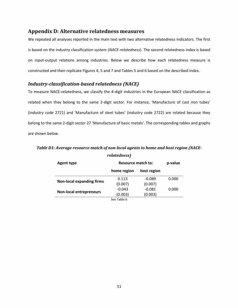
51
Appendix D: Alternative relatedness measures
We repeated all analyses reported in the main text with two alternative relatedness indicators. The first
is based on the industry classification system (NACE-relatedness). The second relatedness index is based
on input-output relations among industries. Below we describe how each relatedness measure is
constructed and then replicate Figures 4, 5 and 7 and Tables 5 and 6 based on the described index.
Industry-classification-based relatedness (NACE)
To measure NACE-relatedness, we classify the 4-digit industries in the European NACE classification as
related when they belong to the same 2-digit sector. For instance, ‘Manufacture of cast iron tubes’
(industry code 2721) and ‘Manufacture of steel tubes’ (industry code 2722) are related because they
belong to the same 2-digit sector 27 ‘Manufacture of basic metals’. The corresponding tables and graphs
are shown below.
Table D1: Average resource match of non-local agents to home and host region (NACE-
relatedness)
Agent type Resource match to: p-value
home region host region
Non-local expanding firms 0.113
(0.007) -0.089 (0.007)
0.000
Non-local entrepreneurs -0.043 (0.003)
-0.081 (0.003)
0.000
See Table 6
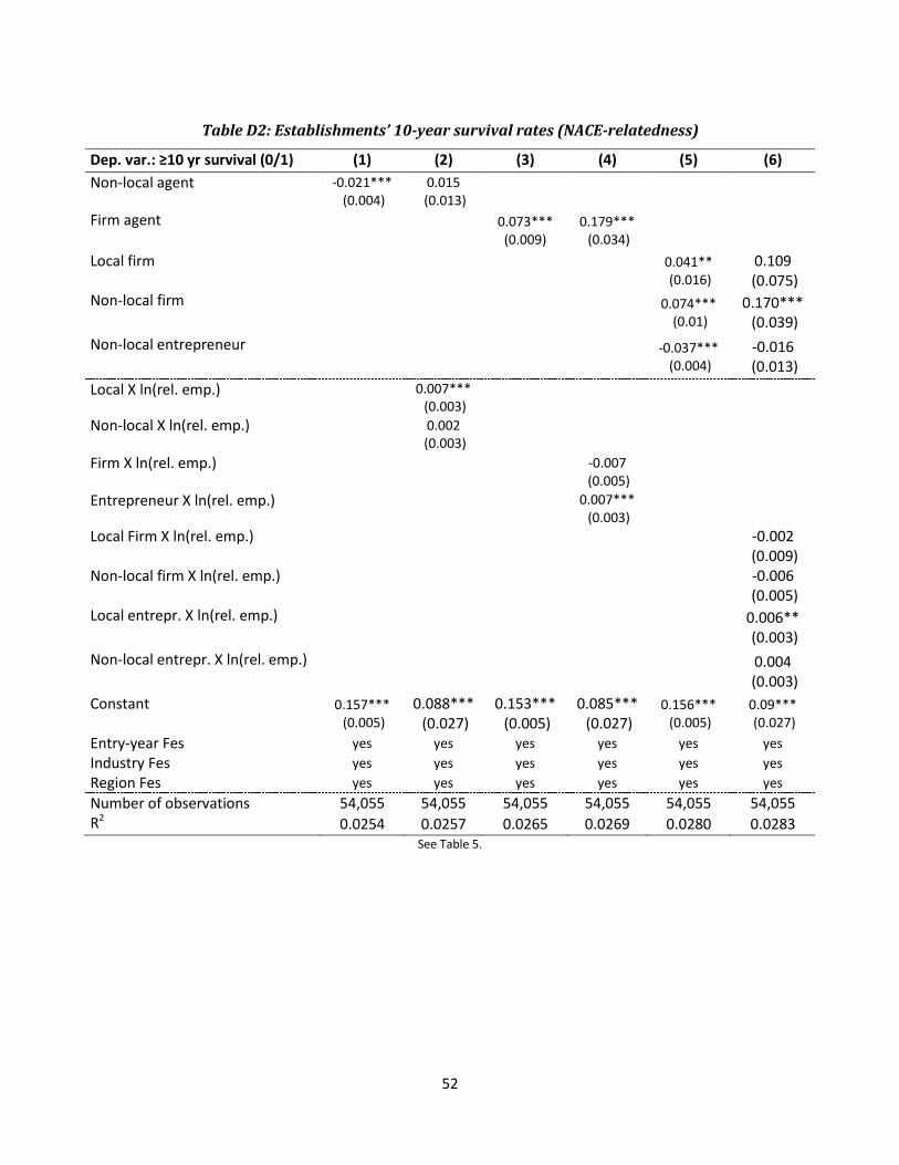
52
Table D2: Establishments’ 10-year survival rates (NACE-relatedness)
Dep. var.: ≥10 yr survival (0/1) (1) (2) (3) (4) (5) (6)
Non-local agent -0.021*** (0.004)
0.015 (0.013)
Firm agent
0.073*** (0.009)
0.179*** (0.034)
Local firm
0.041** (0.016)
0.109 (0.075)
Non-local firm
0.074*** (0.01)
0.170*** (0.039)
Non-local entrepreneur
-0.037*** (0.004)
-0.016 (0.013)
Local X ln(rel. emp.)
0.007*** (0.003)
Non-local X ln(rel. emp.)
0.002 (0.003)
Firm X ln(rel. emp.)
-0.007 (0.005)
Entrepreneur X ln(rel. emp.)
0.007*** (0.003)
Local Firm X ln(rel. emp.)
-0.002 (0.009)
Non-local firm X ln(rel. emp.)
-0.006 (0.005)
Local entrepr. X ln(rel. emp.)
0.006** (0.003)
Non-local entrepr. X ln(rel. emp.)
0.004 (0.003)
Constant 0.157*** (0.005)
0.088*** (0.027)
0.153*** (0.005)
0.085*** (0.027)
0.156*** (0.005)
0.09*** (0.027)
Entry-year Fes yes yes yes yes yes yes
Industry Fes yes yes yes yes yes yes
Region Fes yes yes yes yes yes yes
Number of observations 54,055 54,055 54,055 54,055 54,055 54,055 R2 0.0254 0.0257 0.0265 0.0269 0.0280 0.0283
See Table 5.

53
Figure D1: Coherence of labor market regions’ resource bases (NACE-relatedness)
See Figure 4.
Figure D2: Structural change in Sweden’s labor market regions (NACE-relatedness)
See Figure 5.
-0.4
-0.3
-0.2
-0.1
0
0.1
0.2
0.3
0.41
99
4
19
95
19
96
19
97
19
98
19
99
20
00
20
01
20
02
20
03
20
04
20
05
20
06
20
07
20
08
20
09
20
10
Year
NACE coherence
baseline
-0.15
-0.10
-0.05
0.00
0.05
0.10
0.15
0.20
0.25
0.30
0.35
19
94
19
95
19
96
19
97
19
98
19
99
20
00
20
01
20
02
20
03
20
04
20
05
20
06
20
07
20
08
20
09
20
10
Year
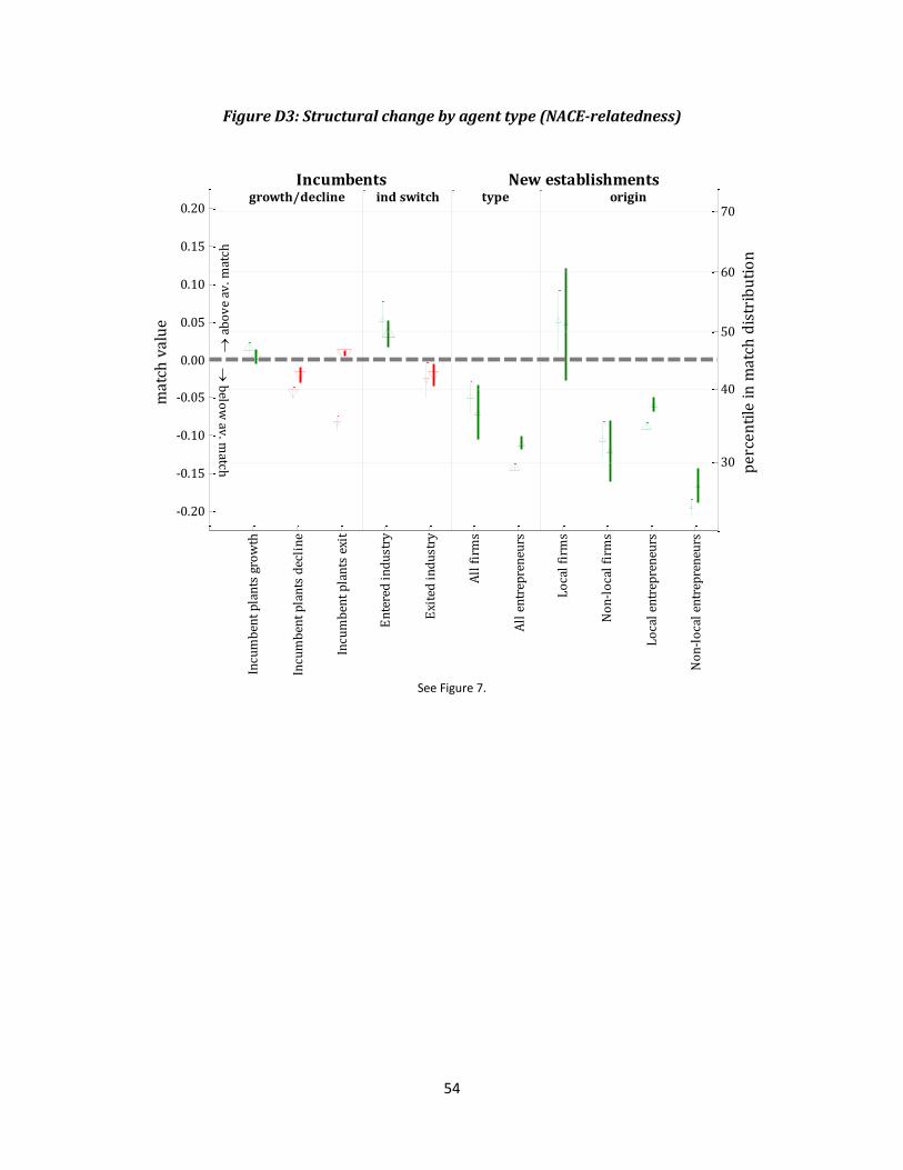
54
Figure D3: Structural change by agent type (NACE-relatedness)
See Figure 7.
-0.20
-0.15
-0.10
-0.05
0.00
0.05
0.10
0.15
0.20
Incu
mb
ent
pla
nts
gro
wth
Incu
mb
ent
pla
nts
dec
lin
e
Incu
mb
ent
pla
nts
exi
t
En
tere
d i
nd
ust
ry
Exi
ted
in
du
stry
All
fir
ms
All
en
trep
ren
eurs
Lo
cal
firm
s
No
n-l
oca
l fi
rms
Lo
cal
entr
epre
neu
rs
No
n-l
oca
l en
trep
ren
eurs
mat
ch v
alu
eIncumbents
growth/decline ind switchNew establishments
type origin
a
bo
ve
av. m
atch
b
elow
av. m
atch 30
40
50
60
70
per
cen
tile
in m
atch
dis
trib
uti
on
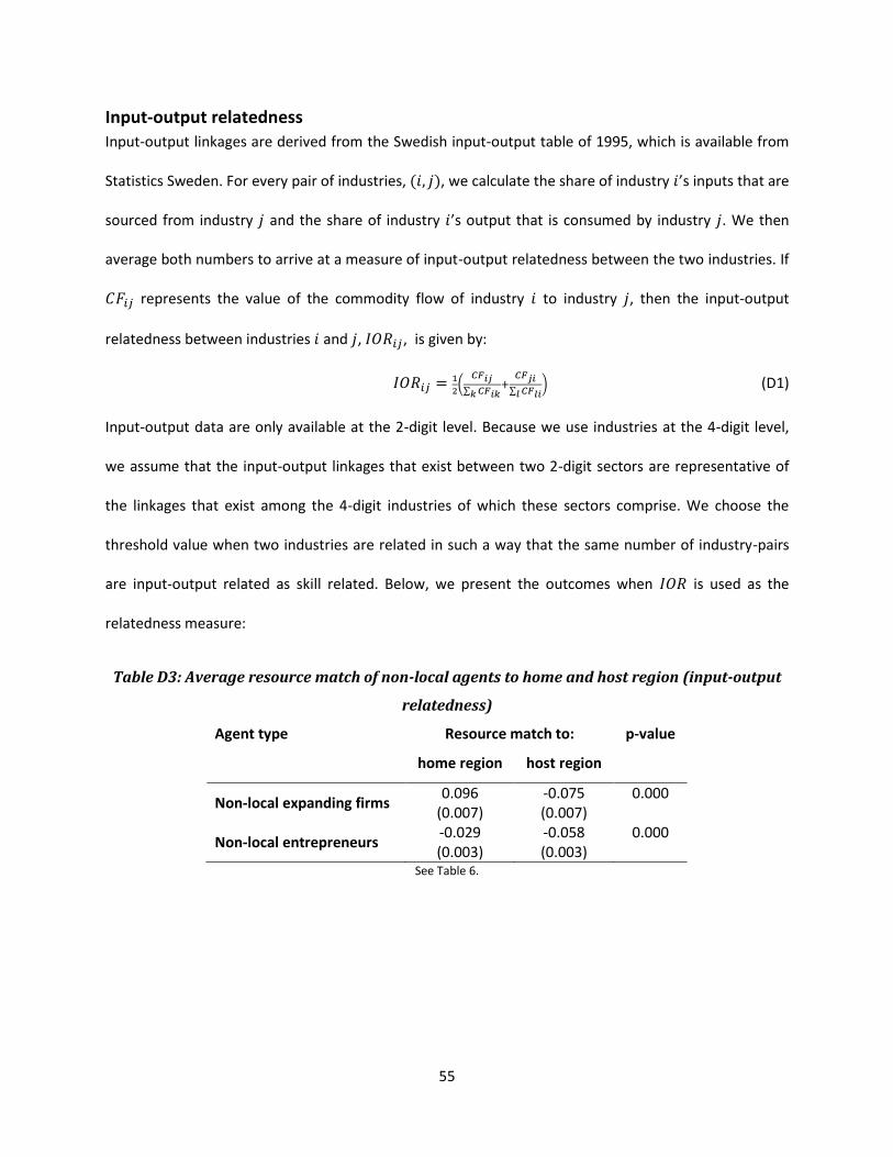
55
Input-output relatedness
Input-output linkages are derived from the Swedish input-output table of 1995, which is available from
Statistics Sweden. For every pair of industries, (𝑖, 𝑗), we calculate the share of industry 𝑖’s inputs that are
sourced from industry 𝑗 and the share of industry 𝑖’s output that is consumed by industry 𝑗. We then
average both numbers to arrive at a measure of input-output relatedness between the two industries. If
𝐶𝐹𝑖𝑗 represents the value of the commodity flow of industry 𝑖 to industry 𝑗, then the input-output
relatedness between industries 𝑖 and 𝑗, 𝐼𝑂𝑅𝑖𝑗, is given by:
𝐼𝑂𝑅𝑖𝑗 = 1
2(
𝐶𝐹𝑖𝑗
∑ 𝐶𝐹𝑖𝑘𝑘+
𝐶𝐹𝑗𝑖
∑ 𝐶𝐹𝑙𝑖𝑙) (D1)
Input-output data are only available at the 2-digit level. Because we use industries at the 4-digit level,
we assume that the input-output linkages that exist between two 2-digit sectors are representative of
the linkages that exist among the 4-digit industries of which these sectors comprise. We choose the
threshold value when two industries are related in such a way that the same number of industry-pairs
are input-output related as skill related. Below, we present the outcomes when 𝐼𝑂𝑅 is used as the
relatedness measure:
Table D3: Average resource match of non-local agents to home and host region (input-output
relatedness)
Agent type Resource match to: p-value
home region host region
Non-local expanding firms 0.096
(0.007) -0.075 (0.007)
0.000
Non-local entrepreneurs -0.029 (0.003)
-0.058 (0.003)
0.000
See Table 6.

56
Table D4: Establishments’ 10-year survival rates (input-output relatedness)
Dep. var.: ≥10 yr survival (0/1) (1) (2) (3) (4) (5) (6)
Non-local agent -0.021*** (0.004)
-0.002 (0.012)
Firm agent
0.073*** (0.009)
0.13*** (0.028)
Local firm
0.041** (0.016)
0.113* (0.061)
Non-local firm
0.074*** (0.01)
0.108*** (0.032)
Non-local entrepreneur
-0.037*** (0.004)
-0.03** (0.012)
Local X ln(rel. emp.)
0.008*** (0.003)
Non-local X ln(rel. emp.)
0.005* (0.003)
Firm X ln(rel. emp.)
0.001 (0.004)
Entrepreneur X ln(rel. emp.)
0.008*** (0.003)
Local Firm X ln(rel. emp.)
-0.001 (0.007)
Non-local firm X ln(rel. emp.)
0.003 (0.004)
Local entrepr. X ln(rel. emp.)
0.007*** (0.003)
Non-local entrepr. X ln(rel. emp.)
0.006** (0.003)
Constant 0.157*** (0.005)
0.073** (0.031)
0.153*** (0.005)
0.067** (0.03)
0.156*** (0.005)
0.078** (0.031)
Entry-year Fes yes yes yes yes yes yes
Industry Fes yes yes yes yes yes yes
Region Fes yes yes yes yes yes yes
Number of observations 54,055 54,055 54,055 54,055 54,055 54,055 R2 0.0254 0.0256 0.0265 0.0268 0.0280 0.0282
See Table 5.
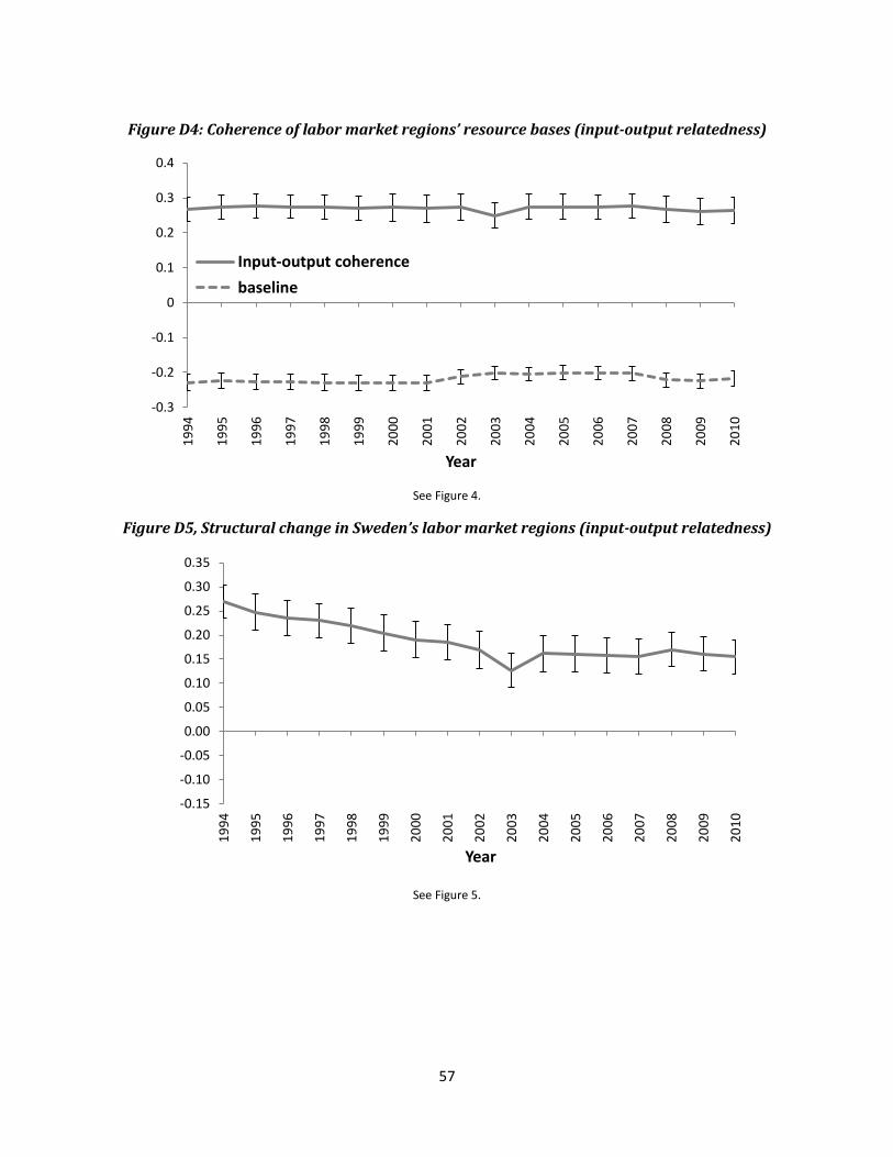
57
Figure D4: Coherence of labor market regions’ resource bases (input-output relatedness)
See Figure 4.
Figure D5, Structural change in Sweden’s labor market regions (input-output relatedness)
See Figure 5.
-0.3
-0.2
-0.1
0
0.1
0.2
0.3
0.4
19
94
19
95
19
96
19
97
19
98
19
99
20
00
20
01
20
02
20
03
20
04
20
05
20
06
20
07
20
08
20
09
20
10
Year
Input-output coherence
baseline
-0.15
-0.10
-0.05
0.00
0.05
0.10
0.15
0.20
0.25
0.30
0.35
19
94
19
95
19
96
19
97
19
98
19
99
20
00
20
01
20
02
20
03
20
04
20
05
20
06
20
07
20
08
20
09
20
10
Year

58
Figure D6: Structural change by agent type (input-output relatedness)
See Figure 7.
-0.20
-0.15
-0.10
-0.05
0.00
0.05
0.10
0.15
0.20
Incu
mb
ent
pla
nts
gro
wth
Incu
mb
ent
pla
nts
dec
lin
e
Incu
mb
ent
pla
nts
exi
t
En
tere
d i
nd
ust
ry
Exi
ted
in
du
stry
All
fir
ms
All
en
trep
ren
eurs
Lo
cal
firm
s
No
n-l
oca
l fi
rms
Lo
cal
entr
epre
neu
rs
No
n-l
oca
l en
trep
ren
eurs
mat
ch v
alu
e
Incumbentsgrowth/decline ind switch
New establishmentstype origin
a
bo
ve
av. m
atch
b
elow
av. m
atch 30
40
50
60
70
per
cen
tile
in m
atch
dis
trib
uti
on


