
UNIVERSITY OF THESSALY
SCHOOL OF ENGINEERING
DEPARTMENT OF MECHANICAL ENGINEERING
AERODYNAMIC DESIGN AND ANALYSIS OF A SOLAR POWERED UAV
(Unmanned Aerial Vehicle)
by
SAVVAS KOKKOS
AND
EFSTRATIOS MORFIDIS

ii
Submitted in partial fulfillment of the requirements for the degree of Diploma
in Mechanical Engineering at the University of Thessaly
Volos, 2020

iii
© 2020 Savvas Kokkos, Efstratios Morfidis
All rights reserved. The approval of the presented Thesis by the Department of Mechanical Engineering, School of Engineering, University of Thessaly, does not imply acceptance of the views of the author (Law 5343/32 art. 202).

iv
Approved by the Committee on Final Examination:
Advisor Dr. Pelekasis Nikolaos,
Professor, Department of Mechanical Engineering,
University of Thessaly
Member Dr. Bontozoglou Vasilis,
Professor, Department of Mechanical Engineering,
University of Thessaly
Member Dr. Stamatelos Anastasios,
Professor, Department of Mechanical Engineering,
University of Thessaly
Date Approved: [February , 2020]
v
AERODYNAMIC DESIGN AND ANALYSIS OF A SOLAR POWERED
UAV (Unmanned Arial Vehicle)
SAVVAS KOKKOS
EFSTRATIOS MORFIDIS
Department of Mechanical Engineering, University of Thessaly, 2020
Supervisor: Dr Nikolaos Pelekasis
Professor of Computational Fluid Dynamics
Abstract
This thesis studies the design of a solar powered unmanned aerial vehicle (UAV) with
maximum altitude 2000 m that can complete a whole 24 h flight. The analysis uses sun data
of the summer season in Greece and by making a first estimation of lift and drag coefficients
the study that follows proves that theoretically the concept can be achieved. Besides the sun
data the electrical components with the whole composite material weight was estimated
using an EXCEL spreadsheet. Having selected the 2D airfoil profiles the study uses the XFLR5
environment to extract the lift and drag coefficients of an arbitrary wing with planform bottom
view and then utilizes initially the lifting line theory to get an estimation of the wing
aerodynamic behavior. Then the comparison, based on efficiency criteria with the most
important one to be the watt consumption of the drag force, takes place and the airfoil that
best matches the preferences of the project is used to create the 3D wing. For the validation
of the results an experimental setup that calculates the pressure distribution over a 2D foil
was introduced but left as future work. After reaching a mesh independent solution using the
ANSYS Fluent environment the aero map of the wing was calculated and used to define the
optimal Angle of Attack of the selected wing. At this time the fuselage design takes place and
comparing the types of the fuselages that Gundmundson introduces two concepts were

vi
chosen. Further study took place in order to achieve the elliptical lift distribution to eliminate
the induced drag and the final design of the fuselage the one with embedded wings was
finalized. Then knowing the place of the center of pressure and the position of the center of
mass, using the xflr5 environment after the stability analysis took place the final geometrical
parameters of the tail were calculated and the whole UAV was finalized. As future work has
been left the PID tuning of the control surfaces and the experimental setup validation.
Key words: Solar powered UAV, Solar Energy, Solar Airplane, Sustainable Flight

vii
ΑΕΡΟΔΥΝΑΜΙΚΟΣ ΣΧΕΔΙΑΣΜΟΣ ΚΑΙ ΑΝΑΛΥΣΗ ΗΛΙΟ-ΤΡΟΦΟΔΟΤΟΥΜΕΝΟΥ MEA
(Μη Επανδρωμένο Αεροσκάφος)
ΣΑΒΒΑΣ ΚΟΚΚΟΣ
ΕΥΣΤΡΑΤΙΟΣ ΜΟΡΦΙΔΗΣ
Τμήμα Μηχανολόγων Μηχανικών, Πανεπιστήμιο Θεσσαλίας, 2020
Επιβλέπων Καθηγητής: Δρ. Νικόλαος Πελεκάσης,
Καθηγητής Υπολογιστικής Ρευστοδυναμικής
Περίληψη
Στην παρούσα διπλωματική εργασία μελετάται ο αεροδυναμικός σχεδιασμός ενός
ηλιοτροφοδοτούμενου μη επανδρωμένου αεροσκάφους με ικανότητα πτήσης έως 2000 m,
το οποίο καλείται να ολοκληρώσει μια πτήση 24 ωρών. Η ανάλυση που ακολουθεί
χρησιμοποιεί δεδομένα ηλιακής ακτινοβολίας κατα τις καλοκαιρινές περιόδους στην Ελλάδα
και με μία πρώτη εκτίμηση των αεροδυναμικων συντελεστών οπισθέλκουσας και άνωσης η
ανάλυση αποδεικνύει ότι θεωρητικά ο στόχος μπορεί να επιτευχθεί. Μετά από έναν
ενδελεχή προσδιορισμό του βάρους όλων των ηλεκτρονικών κομματιών που θα
χρησιμοποιηθούν καθώς και του βάρους της κατασκευής αυτής καθαυτής γίνεται μία αρχική
εκτίμηση του βάρους του μη επανδρωμένου οχήματος. Μετά από την συγκέντρωση
αεροτομών που σαν κύριο χαρακτηρηστικό έχουν την μεγάλη απόδοση χρησιμοποιήθηκε το
περιβάλλον του XFLR5 προκειμένου να προσδιοριστούν οι διδυαστατοι αεροδυναμικοί
συντελεστές της εκάστωτε αεροτομής και εν συνεχεία με την χρήση της μεθόδου της γραμμής
άνωσης προσδιορίσθηκαν τα χαρακτηρηστικά ενός φτερου ορθογωνικής κάτοψης που έχει
την αντίστοιχη αεροτομή σαν προφιλ. Έχοντας θέσει κάποια κριτήρια σχετικά με την
απόδοση των αεροτομών ακολουθεί μια σύγκριση αυτών προκειμένου να επιλεγεί η πίο
κατάλληλη για το πρότζεκτ μας. Φυσικά επειδή η θεωρία απέχει από την πραγματικότητα
προτάθηκε μια πειραματική διάταξη η οποία υπολογίζει το προφίλ των πιέσεων πάνω από

viii
μια πτέρυγα, κάτι το οποίο όμως αφέθηκε για να γίνει στο μέλλον. Σε αυτό το σημείο όλοι οι
υπολογισμοί που έλαβαν χώρα δεν είχαν συνυπολογίσει την συμμετοχή της τριβής μεταξύ
του ρευστού και των μοντέλων μας στραφήκαμε στο ANSYS προκειμένου να
χρησιμοποιήσουμε ένα μοντέλο τύρβης και να εξάγουμε έναν χάρτη των αεροδυναμικών
δυνάμεων προκειμένου να καθορίσουμε την βέλτιστη γωνία προσβολής της πτέρυγας.
Ακολουθώντας τις προτάσεις του Gundmundson για το είδος της ατράκτου που μπορεί να
χρησιμοποιηθεί συγκρίναμε 2 είδη. Το πρώτο είναι κυλινδρικό ενώ το δεύτερο έχει
ενσωματωμένες τις πτέρυγες με τον κυρίως κορμό. Επεκτείναμε την μελέτη των παραμέτρων
της πτέρυγας και αλλάξαμε γεωμετρικά χαρακτηρηστικά όπως την συστροφή το είδος και το
πάχος της αεροτομής προκειμένου να επιτύχουμε την ελλειπτική κατανομή της άνωσης κατα
μήκος του εκπετάσματος του φτερού καταφέρνοντας να εκμηδενίσουμε την επαγώμενη
συνιστώσα της οπισθέλκουσας δύναμης. Έχοντας πλέον στα χέρια μας την θέση του κέντρου
βάρους και του κέντρου πίεσης μπορούμε πλέον να ολοκληρώσουμε τον σχεδιασμό με την
οριστικοποίηση των διαστάσεων της ουράς του μη επανδωμένου οχήματος στέφοντας την
προσοχή μας στην ανάλυση ευστάθειας μέσω του προγράμματος XFLR5. Σαν μελλοντική
δουλειά αφέθηκε η εκτέλεση του πειράματος που προτάθηκε ανωτέρω καθώς και η
βελτιστοποίηση των ενισχύσεων του PID ελεγκτή για τις κινητές επιφάνειες ελέγχου.
Λέξεις-κλειδιά:
ix
Table of Contents Chapter1: Introduction .................................................................................................. 1
1.1. Motivation and Objectives ....................................................................................................... 1
1.2. History of Solar Powered Flight ................................................................................................ 2
1.2.1. : The Conjunction of two Pioneer Fields, Electric Flight and Solar Cells ................................ 2
1.2.2. Early Stages of Solar Aviation with Model Airplane .............................................................. 2
1.2.3. The Dream of Manned Solar Flight ........................................................................................ 4
1.2.4. On the Way to High Altitude Long Endurance Platforms and Eternal Flight ......................... 7
1.3. Basic Principles ...................................................................................................................... 11
1.3.1. Airplane Aerodynamics ........................................................................................................ 11
1.3.2. Airfoil Dynamics ................................................................................................................... 12
1.4. Type of UAVs ......................................................................................................................... 15
1.4.1. Monoplane .......................................................................................................................... 15
1.4.2. VTOL Vehicles ...................................................................................................................... 16
1.4.3. Multicopters ........................................................................................................................ 16
Chapter2: Preliminary Analysis .................................................................................... 18
2.1 Solar Irradiance in Greece ...................................................................................................... 18
2.1.1. Solar Cell Selection .............................................................................................................. 19
2.2. UAV Type Selection ................................................................................................................ 22
2.3. Initial Sizing ............................................................................................................................ 23
2.3.1. Lifting Line Theory(LLT) ........................................................................................................ 25
2.3.2. High Lift Devices .................................................................................................................. 29
2.3.3. Weight Estimation ............................................................................................................... 30
Chapter3: 2D Analysis ................................................................................................. 34
3.1. 2D simulations ....................................................................................................................... 34
3.2. Selection Criteria and 2D Airfoil Comparison ......................................................................... 37
3.2.1. 2D to 3D Estimation ............................................................................................................. 39
3.3. Airfoil Comparison and Rejection Stages ................................................................................ 40
3.4. Experimental Setup ................................................................................................................ 49
Chapter4: Wing ........................................................................................................... 55
4.1. Ansys CFD Simulation............................................................................................................. 61
4.1.1. Geometry Preparation ......................................................................................................... 63

x
4.1.2. Meshing ............................................................................................................................... 69
4.1.3. Solving Process .................................................................................................................... 74
4.1.4. Mesh Dependency ............................................................................................................... 88
4.1.5. Results ................................................................................................................................. 91
4.2. 3D Wing Design ...................................................................................................................... 97
4.2.1. Elliptic Distribution .............................................................................................................. 97
4.2.2. Wing Parameters ................................................................................................................. 98
Chapter5: Fuselage..................................................................................................... 106
5.1. Fuselage Types ..................................................................................................................... 107
5.1.1. The Frustum Fuselage ........................................................................................................ 107
5.1.2. The Pressure Tube Fuselage .............................................................................................. 108
5.1.3. Tadpole Fuselage ............................................................................................................... 109
5.1.4. Blended Wing Fuselage ..................................................................................................... 111
5.2. Fuselage Design ................................................................................................................... 112
Chapter6: Tail Design and Stability ............................................................................. 122
6.1. Stable Flight ......................................................................................................................... 122
6.2. Initial Empennage Design ..................................................................................................... 127
6.3. Static Stability ...................................................................................................................... 131
6.4. Dynamic Stability ................................................................................................................. 135
Chapter7: i
7.1. Conclusion ................................................................................................................................ i
7.2. Future work .............................................................................................................................. i
7.2.1. Experimental Setup .................................................................................................................i
7.2.2. Dynamic Simulation with Control Area Sizing and PID Tuning ............................................... ii
Chapter8: APENDIX ...................................................................................................... iii
Chapter9: Bibliography...................................................................................................x

xi
Table of Figures
Figure 1-1: Sunrise I (1974) and Solaris (1976) .......................................................................... 3
Figure 1-2: Solar Excel (1990) and PicoSol (1998) ...................................................................... 4
Figure 1-3: Gossamer Penguin (1980) and its successor, Solar Challenger (1981) .................... 5
Figure 1-4: Icaré 2 (1996) and Solair II (1998) ............................................................................ 6
Figure 1-5: Centurion (1997-1999) and Helios (1999-2003). ..................................................... 8
Figure 1-6: Solitair (1998) and Solong (2005) ............................................................................ 9
Figure 1-7: Zephyr (2005) and the future Solar Impulse .......................................................... 10
Figure 1-8: Forces acting on an airplane at level flight ............................................................ 11
Figure 1-9: Solar airplane basic principle. ................................................................................ 12
Figure 1-10: Section of an airfoil .............................................................................................. 12
Figure 1-11: Lift and drag coefficients depending on the angle of attack ............................... 14
Figure 1-12: VTOL Vehicles ....................................................................................................... 16
Figure 1-13: VTOL Fixed Wing UAV .......................................................................................... 16
Figure 1-14: Quadcopter .......................................................................................................... 17
Figure 1-15: Tricopter ............................................................................................................... 17
Figure 1-16: Octocopter ........................................................................................................... 17
Figure 1-17: Hexacopter ........................................................................................................... 17
Figure 2-1: Solar Irradiance ...................................................................................................... 18
Figure 2-2: Encapsulated Solar Cells ........................................................................................ 21
Figure 2-3: Flexible Solar Cells .................................................................................................. 22
Figure 2-4: Maxeon Gen II ........................................................................................................ 22
Figure 3-1: Kutta's condition .................................................................................................... 34
Figure 3-2: XFLR5 2d simulation Laplace Equation .................................................................. 35
xii
Figure 3-3: Airfoils @ Re=250.000 & AoA from -5 to 15 Simulations ...................................... 36
Figure 3-4: VLM Panels And Circulation Γi ............................................................................... 41
Figure 3-5: Panel ....................................................................................................................... 42
Figure 3-6: Top 4 airfoils ........................................................................................................... 47
Figure 3-7: Cross Section of the 3D printer Airfoil ................................................................... 51
Figure 3-8: Hole diameter comparison .................................................................................... 51
Figure 3-9: Experimental Setup Render ................................................................................... 53
Figure 3-10: 3D printed adapter/goniometer .......................................................................... 54
Figure 3-11: Manometer tube holder ...................................................................................... 54
Figure 4-1: Fundamental definitions of a trapezoidal wing planform ..................................... 55
Figure 4-2: Cl vs AoA of a planform wing for different Aspect Ratios ..................................... 58
Figure 4-3: Counter rotating wingtip vortices .......................................................................... 59
Figure 4-4: Typical diagram of Cl vs AoA .................................................................................. 60
Figure 4-5: Simulation process ................................................................................................. 62
Figure 4-6: Simulation process ................................................................................................. 63
Figure 4-7:Trailing Edge cutoff ................................................................................................. 65
Figure 4-8: Control Volume of the uav without the size boxes ............................................... 68
Figure 4-9: All the faces that boundary conditions will be applied. ........................................ 69
Figure4-10: Unstructured grid .................................................................................................. 70
Figure 4-11: Structured grid ..................................................................................................... 70
Figure 4-12: Typical trias surface mesh .................................................................................... 71
Figure 4-13: Layers generation ................................................................................................. 72
Figure 4-14: Volume mesh ....................................................................................................... 73
Figure 4-15: Solution process ................................................................................................... 75
Figure 4-16: Boundary conditions used ................................................................................... 81

xiii
Figure 4-17 Curved Control Volume Inlet ................................................................................ 82
Figure 4-18: Inlet boundary condition tab ............................................................................... 83
Figure 4-19:Wall boundary condition ...................................................................................... 85
Figure 4-20: Meshing refinement process ............................................................................... 88
Figure 4-21: Lift and Drag vs Volume and Face Cells Size ........................................................ 89
Figure 4-22: Lift and Drag vs Volume and Volume Cells Size ................................................... 90
Figure 4-23: Final mesh characteristics .................................................................................... 91
Figure 4-24: Indicated polar diagram with flow type............................................................... 92
Figure 4-25: PSU Lift vs AoA for different speed values .......................................................... 93
Figure 4-26: PSU Lift vs AoA for different speed values .......................................................... 93
Figure 4-27: PSU Drag vs Angle of attack ................................................................................. 94
Figure 4-28 :PSU Cd vs Angle of attack .................................................................................... 94
Figure 4-29 PSU Cl to Cd ratio .................................................................................................. 95
Figure 4-30 PSU minimum power efficiency factor ................................................................. 95
Figure 4-31: Drag Power vs AoA ............................................................................................... 95
Figure 4-32: PSU drag power consumption ............................................................................. 96
Figure 4-33 : Elliptical vs Rectangular Cl distribution ............................................................... 97
Figure 4-34: Elliptical vs Uniform Lift Distribution ................................................................... 98
Figure 4-35: Wing Design ......................................................................................................... 99
Figure 4-36: Polar type ........................................................................................................... 100
Figure 4-37: Analysis method ................................................................................................. 100
Figure 4-387: Analysis Method .............................................................................................. 100
Figure 4-39: Mass selection of the airplane ........................................................................... 100
Figure 4-40: Orthogonal Shaped Wing & Induced Drag Distribution .................................... 101
Figure 4-41: Orthogonal Wing, Lift Distribution .................................................................... 101
xiv
Figure 4-42: Orthogonal Wing With Horizontal Winglets, Lift Distribution ........................... 102
Figure 4-43: Orthogonal Wing With Horizontal Winglets ...................................................... 102
Figure 4-44: Orthogonal Wing With Horizontal Winglets & Twist, Lift Distribution.............. 103
Figure 4-45: Orthogonal Wing With Horizontal Winglets & Twist ......................................... 103
Figure 4-46: Orthogonal Wing With Horizontal Winglets & Twist, version II ........................ 104
Figure 4-47: Orthogonal Wing With Horizontal Winglets & Twist, version II, Lift Distribution
........................................................................................................................................ 104
Figure 4-48: Orthogonal Wing With Horizontal Winglets & Twist, version III ....................... 105
Figure 4-49: Orthogonal Wing With Horizontal Winglets & Twist, version III, Lift Distribution
........................................................................................................................................ 105
Figure 5-1: 2D fuselage section ............................................................................................. 107
Figure 5-2: Frustum fuselage type ......................................................................................... 108
Figure 5-3: Pressure Tube Fuselage Vs Angle of Attack ......................................................... 108
Figure 5-4: Frustum vs Tadpole Fuselage Ref. Althaus D. Motorless Flight Research .......... 109
Figure 5-5: Upwash effect in the fuselage ............................................................................. 110
Figure 5-6: Aircrafts with Embeded Wings ............................................................................ 111
Figure 5-7: Electronics Assembly............................................................................................ 112
Figure 5-8: Electronics Assembly Zoomed In ......................................................................... 112
Figure 5-9: Tadpole/Cylindrical Fuselage ............................................................................... 113
Figure 5-10: Electronics Assembly with Sketched Fuselage Around Them ........................... 113
Figure 5-11: Tadpole/Cylindrical Fuselage ............................................................................. 114
Figure 5-12: Tadpole/Cylindrical Fuselage with Wings Attached .......................................... 114
Figure 5-13: First Blended Wing Design & It's Lift Distribution ............................................. 115
Figure 5-14: 2nd Design Lift Distribution ................................................................................. 116
Figure 5-15: 3rd Design Lift Distribution ................................................................................. 116

xv
Figure 5-16: 4th Design Lift Distribution ................................................................................. 117
Figure 5-17: Final Design Lift Distribution .............................................................................. 118
Figure 5-18: Final Assembly With Electrical Components ..................................................... 119
Figure 5-19: Blended Wing ..................................................................................................... 120
Figure 5-20: Blended Wing Fuselage Concept ....................................................................... 121
Figure 5-21: Tadpole/Cylindrical Concept .............................................................................. 120
Figure 6-1: Two different scenarios at high AoA and small AoA............................................ 123
Figure 6-2: Plot of the two scenarios Cm vs AoA ................................................................... 125
Figure 6-3: Initial empennage sizing ...................................................................................... 128
Figure 6-4: Tail volume coefficients ....................................................................................... 128
Figure 6-5: AoA = -3o .............................................................................................................. 131
Figure 6-6: AoA = -1o .............................................................................................................. 132
Figure 6-7: AoA = -2o .............................................................................................................. 132
Figure 6-8: AoA = 1o ................................................................................................................ 133
Figure 6-9: AoA=0o ................................................................................................................. 133
Figure 6-10: Cm vs AoA in final empennage design ............................................................... 134
Figure 6-11: AoA = 2 o ............................................................................................................. 134
Figure 6-12: Phugoid modes .................................................................................................. 135
Figure 6-13: Short period modes ........................................................................................... 136
Figure 6-14: Spiral mode ........................................................................................................ 137
Figure 6-15: Roll damping mode ............................................................................................ 138
Figure 6-16: Ditch roll modes ................................................................................................. 139
Figure 196-17: Longitudinal mode I, Short period mode ....................................................... 140
Figure 6-18:Longitudinal mode II, Short period mode ........................................................... 141
Figure 6-19:Longitudinal mode III & IV, Phugoid modes ....................................................... 142

xvi
Figure 6-20:Lateral mode I, Roll damping mode .................................................................... 143
Figure 6-21:Lateral mode II & III, Dutch roll modes ............................................................... 144
Figure 6-22:Lateral mode IV, Spiral mode.............................................................................. 145
Figure 6-23: Root locus diagram for eigenvalues ................................................................... 146
Figure 7-1:Aquila9.3 .................................................................................................................. iii
Figure 7-2:E374 ......................................................................................................................... iii
Figure 7-3:E387 ......................................................................................................................... iii
Figure 7-4:EH2_10 ..................................................................................................................... iii
Figure 7-5:EPPLER423................................................................................................................ iii
Figure 7-6:FX63137 ................................................................................................................... iv
Figure 7-7:HQ3-8B ..................................................................................................................... iv
Figure 7-8:HS3_9 ....................................................................................................................... iv
Figure 7-9:LA2573A ................................................................................................................... iv
Figure 7-10:LKH2411 ................................................................................................................. iv
Figure 7-11:MEDIUM_S9000(9%) ............................................................................................. iv
Figure 7-12: NACA2412 .............................................................................................................. v
Figure 7-13:NACA63412 ............................................................................................................. v
Figure 7-14:NH1036 ................................................................................................................... v
Figure 7-15:NLF0215F ................................................................................................................ v
Figure 7-16:NLF1015 .................................................................................................................. v
Figure 7-17:OA209 ..................................................................................................................... v
Figure 7-18:PHOENIX ................................................................................................................. vi
Figure 7-19:PSU94-097 .............................................................................................................. vi
Figure 7-20:S510 ........................................................................................................................ vi
Figure 7-21:S905 ........................................................................................................................ vi

xvii
Figure 7-22:SELIG1223 .............................................................................................................. vi
Figure 7-23:S9037......................................................................................................................vii
Figure 7-24:SA7038 ...................................................................................................................vii
Figure 7-25:SD7032 ...................................................................................................................vii
Figure 7-26:SG6040 ...................................................................................................................vii
Figure 7-27:SG6042 .................................................................................................................. viii
Figure 7-28:WE3.55 .................................................................................................................. viii
Figure 7-29: Final UAV Design .................................................................................................. viii
Figure 7-30: Final Airplane ....................................................................................................... viii

1 | P a g e
Chapter1: Introduction
1.1. Motivation and Objectives
The field of application of energy autonomous UAV is extremely wide. Worldwide
there are examples of its application like Human rescue situations, wildlife surveillance, fire
detection, observation of inaccessible territories for example radioactive areas as also
emissions measurement.
These applications would require remaining airborne during days, weeks or even
months. For the moment, it is only possible to reach such ambitious goals using electric solar
powered platform. Photovolataic modules may be used to collect the energy of the sun during
the day, one part being used directly to power the propulsion unit and onboard instruments,
the other part being stored for the night time.
The design manufacturing of an UAV underlies a huge field of study and parts that need
to be taken into consideration for making a project like this take flesh and bone. The whole
project needs to be split into objectives to be studied separately and in combination with each
other since there are compensations to be done in order to find a setup-solution to meet our
goal. The goal will be the endurance of the flight off duty which means that the primal goal is
the 24-hour flight. If this goal achieved, it is very possible that the duration of the fight will be
defined from the sunlight day after day.
The field of the applications is such that a quick responsiveness is not required
and in our case will be avoided. The big deal in our case is the steady flight with an acceptable
range of flight weather conditions. In terms of automatic control and stability we want our
system to be robust, aerodynamically efficient and to have the tendency to reject external
disturbances that can be caused from wind fluctuations, with as smaller flight controller’s
interference as possible.

2 | P a g e
1.2. History of Solar Powered Flight
1.2.1. The Conjunction of two Pioneer Fields, Electric Flight and Solar Cells
The use of electric power for flight vehicles propulsion is not new. The first one was
the hydrogen-filled dirigible France in year 1884 that won a 10 km race around Villacoulbay
and Medon. At this time, the electric system was superior to its only rival, the steam engine,
but then with the arrival of gasoline engines, work on electrical propulsion for air vehicles was
abandoned and the field lay dormant for almost a century. On the 30th of June 1957, Colonel
H. J. Taplin of the United Kingdom made the first officially recorded electric powered radio
controlled flight with his model "Radio Queen", which used a permanent-magnet motor and
a silver-zinc battery. Unfortunately, he didn’t carry on these experiments. Further
developments in the field came from the great German pioneer, Fred Militky, who first
achieved a successful flight with an uncontrolled model in October1957. Since then, electric
flight continuously evolved with constant improvements in the fields of motors and batteries.
Three years before Taplin and Militky’s experiments, in 1954, photovoltaic technology was
born at Bell Telephone Laboratories. Daryl Chapin,Calvin Fuller, and Gerald Pearson developed
the first silicon photovoltaic cell capable of converting enough of the sun’s energy into power
to run every day electrical equipment. First at 4 %, the efficiency improved rapidly to 11%.Two
more decades will be necessary to see the solar technology used for the propulsion of electric
model airplanes.
1.2.2. Early Stages of Solar Aviation with Model Airplane
On the 4th of November 1974, the first flight of a solar powered aircraft took place on
the dry lake at Camp Irwin, California. Sunrise I, designed by R.J.Boucher from Astro Flight Inc.
under a contract with ARPA, flew 20 minutes at an altitude of around 100m during its
inaugural flight. It had a wing span of 9.76 m, weighed 12.25 kg and the power output of the
4096 solar cells was450W. Scores of flights for three to four hours were made during the
winter, but Sunrise I was seriously damaged when caught flying in a sandstorm. Thus, an
improved version, Sunrise II, was built and tested on the12th of September 1975. With the
same wingspan, its weight was reduced to10.21 kg and the 4480 solar cells were able this time
to deliver 600W thanks to their 14% efficiency. After many weeks of testing, this second
3 | P a g e
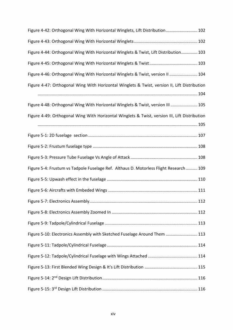
version was also damaged due to a failure in the command and control system. Despite all,
the history of solar flight was engaged and its first demonstration was done.
Figure 1-1: Sunrise I (1974) and Solaris (1976)
On the other side of the Atlantic, Helmut Bruss was working in Germany on a solar
model airplane in summer 1975 without having heard anything about Boucher’s project.
Unluckily, due to overheating of the solar cells on his model, he didn’t achieve level flight and
finally the first one in Europe was his friend Fred Militky, one year later, with Solaris. On the
16th of August 1976, it completed three flights of 150 seconds reaching the altitude of 50m.
Since this early time, many model airplane builders tried to fly with solar energy, this passion
becoming more and more affordable. Of course, at the beginning, the autonomy was limited
to a few seconds, but it rapidly became minutes and then hours. Some people distinguished
themselves like Dave Beck from Wisconsin,USA, who set two records in the model airplane
solar category F5 open SOLof the FAI. In August 1996, his Solar Solitude flew a distance of
38.84kmin straight line and two years later, it reached the altitude of 1283m.The master of
the category is still Wolfgang Schaeper who holds now all the official records: duration (11h
34min 18s), distance in a straight line(48.31 km), gain in altitude (2065 m), speed (80.63 km/h),
distance in a closed-circuit (190 km) and speed in a closed circuit (62.15 km/h). He achieved
these performances with Solar Excel from 1990 to 1999 in Germany.
4 | P a g e
.
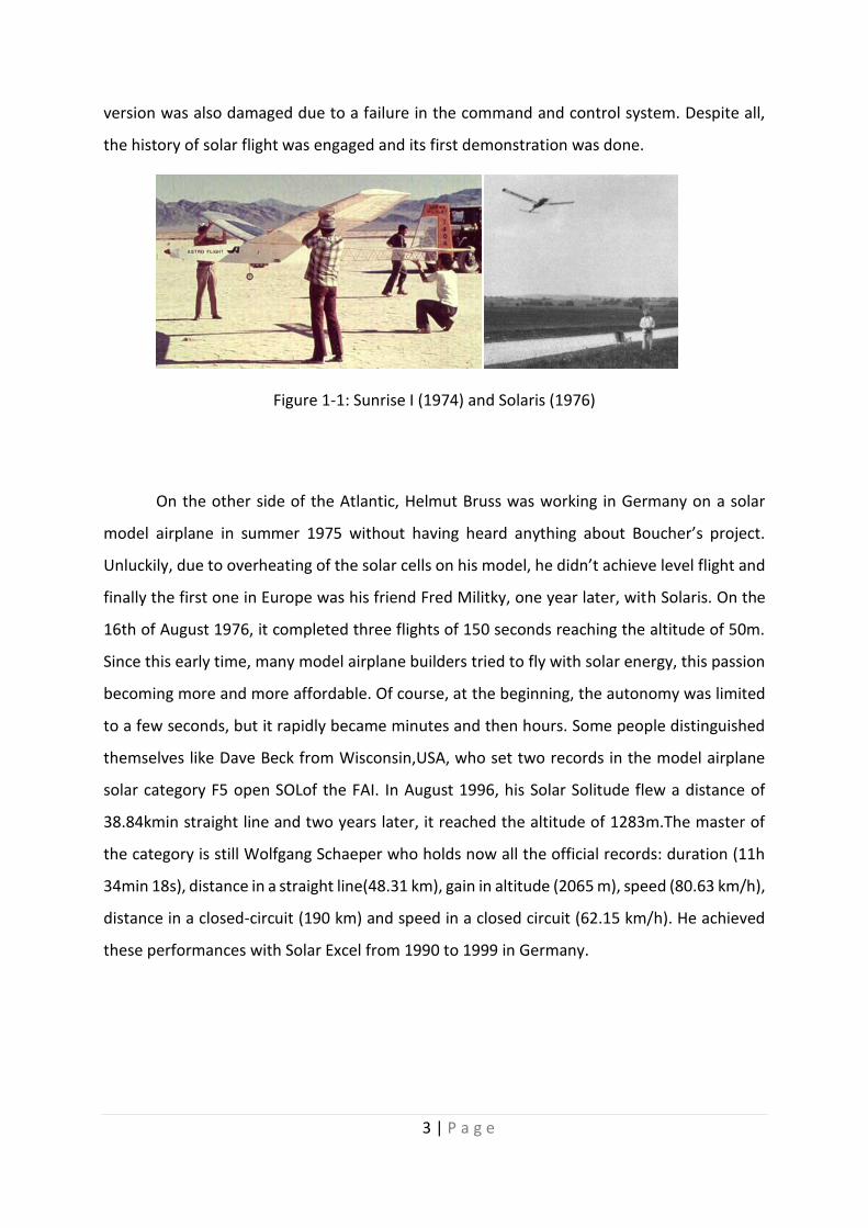
Figure 1-2: Solar Excel (1990) and PicoSol (1998)
We can mention as well the miniature models MikroSol, PicoSol and NanoSol of Dr.
Sieghard Dienlin. PicoSol, the smallest one, weighs only 159.5 g for a wingspan of 1.11m and
its solar panels can provide 8.64 W.
1.2.3. The Dream of Manned Solar Flight
After having flown solar model airplanes and proved it was feasible with sufficient
illumination conditions, the new challenge that fascinated the pioneers at the end of the 70’s
was manned flights powered solely by the sun. On the 19th of December 1978, Britons David
Williams and Fred Tolaunched Solar One on its maiden flight at Lasham Airfield, Hampshire.
First intended to be human powered in order to attempt the Channelcrossing, this
conventional shoulder wing monoplane proved too heavy and thus was converted to solar
power. The concept was to use nickel-cadmium battery to store enough energy for short
duration flights. Its builder was convinced that with high-efficiency solar cells like the one used
on Sunrise, he could fly without need of batteries, but their exorbitant price was the onlylimit.
On April 29, 1979, Larry Mauro flew for the first time the Solar Riser, a solar version of his Easy
Riser hang glider, at Flabob Airport, California. The 350Wsolar panel didn’t have sufficient
power to drive the motor directly and was here again rather used as a solar battery charger.
After a three hours charge the nickel-cadmium pack was able to power the motor for about
ten minutes. His longest flight covered about 800m at altitudes varying between1.5m and
5m.This crucial stage consisting in flying with the sole energy of the sun without any storage
was reached by Dr. Paul B. McCready and AeroVironmentInc, the company he founded in 1971
in Pasadena, California. After having demonstrated, on August 23, 1977, sustained and
5 | P a g e
maneuverable human-powered flight with the Gossamer Condor, they completed on June12,
1979 a crossing of the English Channel with the human-powered GossamerAlbatross. After
these successes, Dupont sponsored Dr. MacCreadyin an attempt to modify a smaller version
of the Gossamer Albatross, called Gossamer Penguin, into a man carrying solar plane. R.J.
Boucher, designer of Sunrise I and II, served as a key consultant on the project. He provided
the motor and the solar cells that were taken from the two damaged versions of Sunrise. On
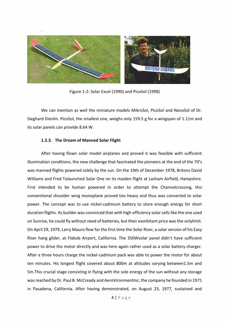
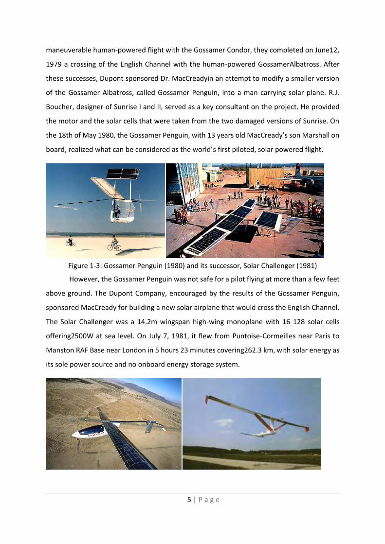
the 18th of May 1980, the Gossamer Penguin, with 13 years old MacCready’s son Marshall on
board, realized what can be considered as the world’s first piloted, solar powered flight.
Figure 1-3: Gossamer Penguin (1980) and its successor, Solar Challenger (1981)
However, the Gossamer Penguin was not safe for a pilot flying at more than a few feet
above ground. The Dupont Company, encouraged by the results of the Gossamer Penguin,
sponsored MacCready for building a new solar airplane that would cross the English Channel.
The Solar Challenger was a 14.2m wingspan high-wing monoplane with 16 128 solar cells
offering2500W at sea level. On July 7, 1981, it flew from Puntoise-Cormeilles near Paris to
Manston RAF Base near London in 5 hours 23 minutes covering262.3 km, with solar energy as
its sole power source and no onboard energy storage system.

6 | P a g e
As they were in England, the members of the Solar Challenger team were surprised to
hear for the first time about a German competitor who was trying to realize exactly the same
performance at the same time from Biggin Hill airport. Günter Rochelt was the designer and
builder of Solair I, a 16m wingspan solar airplane based on the Canard 2FL from AviaFiber that
he slightly modified and covered with 2499 solar cells providing 1800 W. He invited members
of the Solar Challenger team to visit him and R.J. Boucher, who accepted the invitation, was
very impressed by the quality of the airplane. However, with a little more than half the wing
area of solar cells, Solair I didn’t have enough energy to climb and thus incorporated a 22.7 kg
nickel-cadmium battery. Rochelt didn’t realize the Channel crossing this year but on the 21st
of August 1983 he flew in Solair I, mostly on solar energy and also thermals, rising currents of
warm air, during 5 hours 41 minutes. In 1986, Eric Raymond started the design of the
Sunseeker in the United States. The Solar Riser in 1979, Solar Challenger two years later and
a meeting with Günter Rochelt in Germany had convinced him to build his own manned solar
powered aircraft. At the end of 1989, the Sunseeker was test flown as a glider and during
August 1990, it crossed the USA in 21 solar powered flights with 121 hours in the air.
.
Figure 1-4: Icaré 2 (1996) and Solair II (1998)
In Germany, the town of Ulm organized regularly aeronautical competitions in the
memory of Albrecht Berblinger, a pioneer in flying machines200 years ago. For the 1996 event,
they offered attractive prizes to develop a real, practically usable solar aircraft that should be
able to stay up with at least half the solar energy a good summer day with clear sky can give.
This competition started activities round the Earth and more than 30 announced projects, but

7 | P a g e
just some arrived and only one was ready to fly for the final competition. On the 7th of July,
the motor glider Icaré 2 of Prof. Rudolf Voit-Nitschmann from Stuttgart University won the
100,000DM price. Two other interesting competitors were O Sole Mio from the Italian team
of Dr. Antonio Bubbico and Solair II of the team of Prof. Günter Rochelt who took profit of the
experiences gained with the Solair I. Both projects were presented in an advanced stage of
development, but were not airworthy at the time of the competition. The first flight of Solair
II took place two years later in May 1998.
1.2.4. On the Way to High Altitude Long Endurance Platforms and Eternal Flight
After the success of Solar Challenger, the US government gave funding to
AeroVironment Inc. to study the feasibility of long duration, solar electric flight above 19
812km (65 000 ft). The first prototype HALSOL proved the aerodynamics and structures for
the approach, but it suffered from its subsystem technologies, mainly for energy storage, that
were inadequate for this type of mission. Thus, the project took the direction of solar
propulsion with the Pathfinder that achieved its first flight at Dryden in 1993. When funding
for this program ended, the 30m wingspan and 254 kg aircraft became a part of NASA’s
Environmental Research Aircraft Sensor Technology (ERAST) program that started in 1994. In
1995, it exceeded Solar Challenger’s altitude record for solar powered aircraft when it reached
15392m (50 500 ft) and two years later he set the record to 21 802m (71 530 ft). In 1998,
Pathfinder was modified into a new version, Pathfinder Plus, which had a larger wingspan and
new solar, aerodynamic, propulsion and system technologies. The main objective was to
validate these new elements before building its successor, the Centurion. Centurion was
considered to be a prototype technology demonstrator fora future fleet of solar powered
aircrafts that could stay airborne for weeks or months achieving scientific sampling and
imaging missions or serving as telecommunications relay platforms [17]. With a double
wingspan compared to Pathfinder, it was capable to carry 45 kg of remote sensing and data
collection instruments for use in scientific studies of the Earth’s environment and also 270 kg
of sensors, telecommunications and imaging equipment up to24 400m (80 000 ft) altitude. A
lithium battery provided enough energy to the airplane for two to five-hour flight after sunset,
but it was insufficient to fly during the entire night.

8 | P a g e
.
Figure 1-5: Centurion (1997-1999) and Helios (1999-2003).
The last prototype of the series designated as Helios was intended to be the ultimate
"eternal airplane", incorporating energy storage for night-time flight. For NASA, the two
primary goals were to demonstrate sustained flight at an altitude near 30 480m (100 000 ft)
and flying non-stop for at least 24 hours, including at least 14 hours above 15 240m (50 000
ft). In 2001, Helios achieved the first goal near Hawaii with an unofficial world-record altitude
of 29 524m (96 863 ft) and a 40-minute flight above 29 261m (96 000 ft). Unfortunately, it
never reached the second objective as it was destroyed when it fell into the Pacific Ocean on
June 26, 2003 due to structural failures.
In Europe, many projects were also conducted on high altitude, long endurance (HALE)
platforms. At the DLR Institute of Flight Systems, Solitair was developed within the scope of a
study from 1994 to 1998. The solar aircraft demonstrator was designed for year-around
operations in northern European latitude by satisfying its entire onboard energy needs by its
solar panels. So far, a 5.2m wingspan proof-of-concept model aircraft was built with adjustable
9 | P a g e
solar panels for optimum solar radiation absorption. Flight tests were achieved and various
projects are still carried out on this scaled version.
The Helinet project, funded by a European Program, ran between January 2000 and
March 2003 with the target to study the feasibility of a solar powered high altitude platform
of 73m wingspan and 750 kg named Heliplat. It was intended to be used for broadband
communications and Earth observation. The project involved ten European partners and led
to the construction of a 24m wingspan scale prototype of the structure. Politecnico di Torino,
the overall coordinator, is still leading research on Heliplat and also on a new platform named
Shampo.
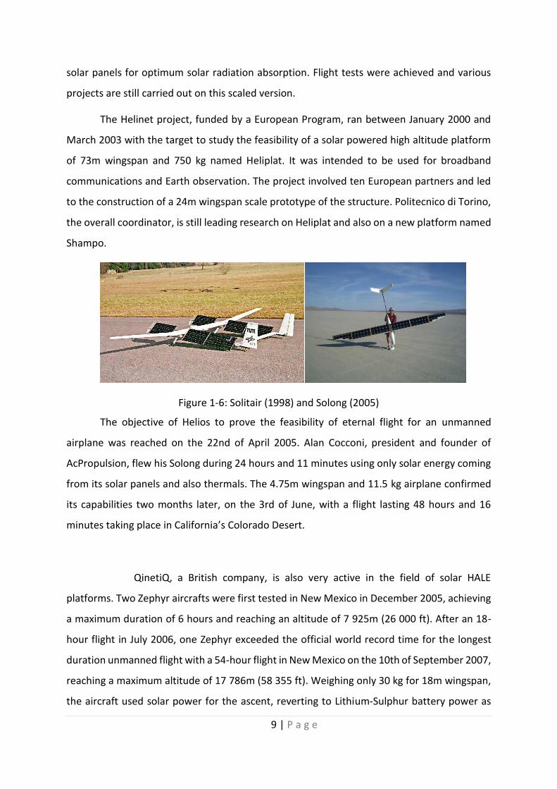
Figure 1-6: Solitair (1998) and Solong (2005)
The objective of Helios to prove the feasibility of eternal flight for an unmanned
airplane was reached on the 22nd of April 2005. Alan Cocconi, president and founder of
AcPropulsion, flew his Solong during 24 hours and 11 minutes using only solar energy coming
from its solar panels and also thermals. The 4.75m wingspan and 11.5 kg airplane confirmed
its capabilities two months later, on the 3rd of June, with a flight lasting 48 hours and 16
minutes taking place in California’s Colorado Desert.
QinetiQ, a British company, is also very active in the field of solar HALE
platforms. Two Zephyr aircrafts were first tested in New Mexico in December 2005, achieving
a maximum duration of 6 hours and reaching an altitude of 7 925m (26 000 ft). After an 18-
hour flight in July 2006, one Zephyr exceeded the official world record time for the longest
duration unmanned flight with a 54-hour flight in New Mexico on the 10th of September 2007,
reaching a maximum altitude of 17 786m (58 355 ft). Weighing only 30 kg for 18m wingspan,
the aircraft used solar power for the ascent, reverting to Lithium-Sulphur battery power as

10 | P a g e
dusk fell. QinetiQ expects in the future flight duration of some months at an altitude above 15
240m (50 000 ft).Zephyr has recently been selected as the base platform for the Flemish
HALE UAV remote sensing system Mercator in the framework of the Pegasus project.
The targeted platform should be able to carry a 100 kg payload in order to fulfill its missions
that are forest fire monitoring, urban mapping, coastal monitoring, oil spill detection and
many others.
Figure 1-7: Zephyr (2005) and the future Solar Impulse
The next dream to prove continuous flight with a pilot on board will perhaps come true
with Solar-Impulse, a project officially announced in Switzerland in 2003. A nucleus of twenty-
five specialists, surrounded by some forty scientific advisors from various universities like
EPFL, is working on the 80m wingspan, 2000 kg lightweight solar airplane. After the
manufacturing of a 60m prototype in 2007-2008 and the final airplane in 2009-2010, a round-
the-world flight should take place in May 2011 with a stopover on each continent.
Of course History is still going on. In early 2007, the DARPA announced the launch of a
new solar HALE project. The Vulture air vehicle program aims at developing the capability to
deliver and maintain a single 453 kg(1000 lbs.), 5 kW airborne payload on station for an
uninterrupted period of at least 5 years.

11 | P a g e
1.3. Basic Principles
1.3.1. Airplane Aerodynamics
Like all other airplanes, a solar airplane has wings that constitute the lifting part.
During steady flight, the airflow due to its relative speed creates two forces: the lift that
maintains the airplane airborne compensating theweight and the drag that is compensated
by the thrust of the propeller.
Figure 1-8: Forces acting on an airplane at level flight
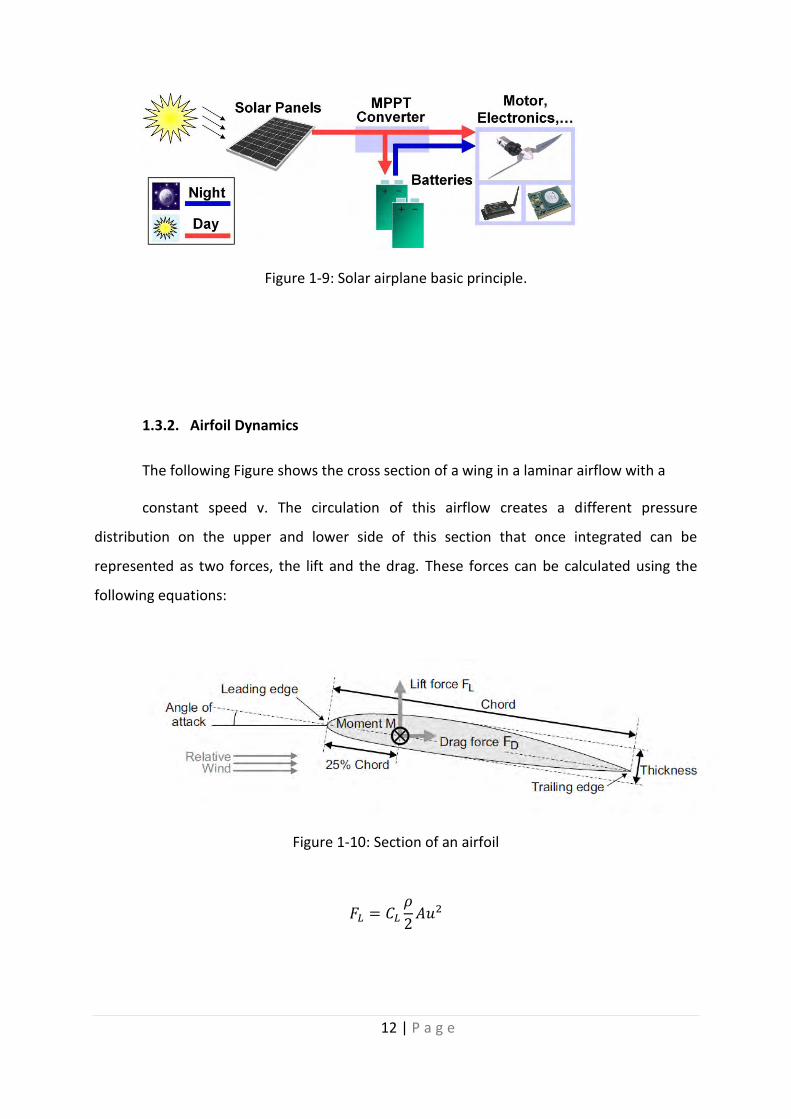
The solar panels, composed by solar cells connected in a defined configuration, cover
a given surface of the wing or potentially other parts of the airplane like the tail or the fuselage.
During the day, depending on the sun irradiance and elevation in the sky, they convert light
into electrical energy. A converter ensures that the solar panels are working at their maximum
power point. That is the reason why this device is called a Maximum Power Point Tracker, that
we will abbreviate MPPT. This power obtained is used firstly to supply the propulsion group
and the onboard electronics, and secondly to charge the battery with the surplus of energy.
12 | P a g e
Figure 1-9: Solar airplane basic principle.
1.3.2. Airfoil Dynamics
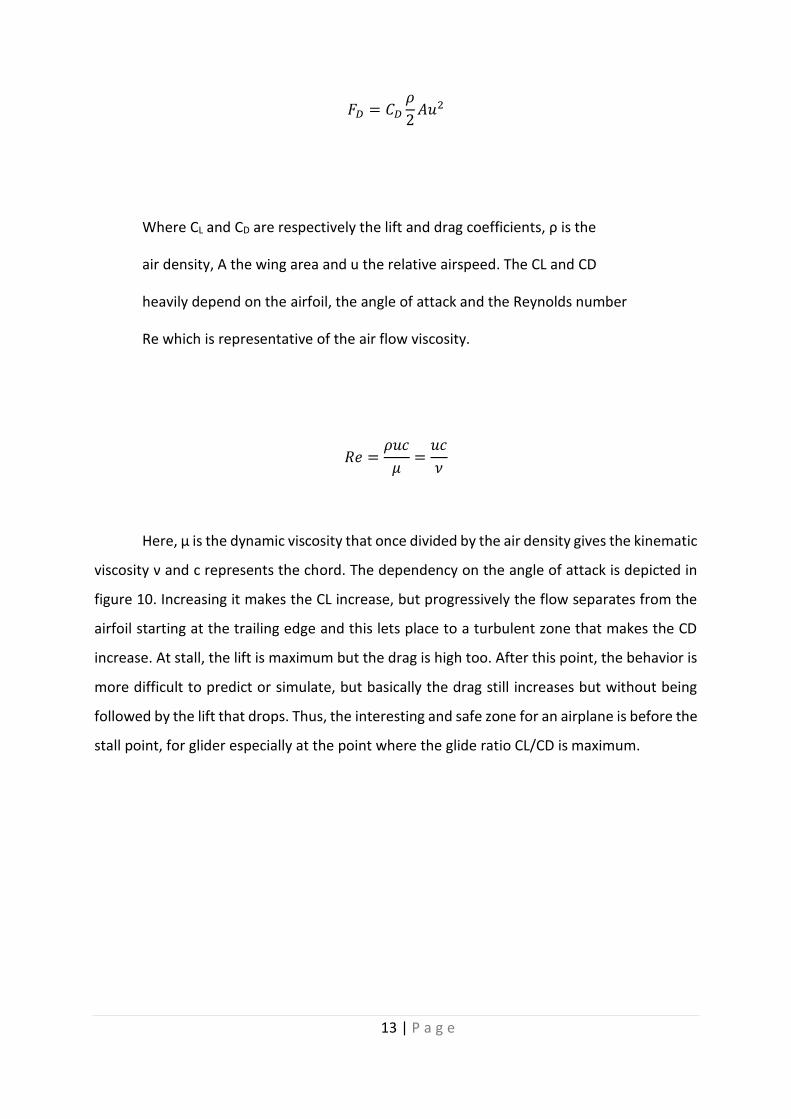
The following Figure shows the cross section of a wing in a laminar airflow with a
constant speed v. The circulation of this airflow creates a different pressure
distribution on the upper and lower side of this section that once integrated can be
represented as two forces, the lift and the drag. These forces can be calculated using the
following equations:
Figure 1-10: Section of an airfoil
𝐹𝐿 = 𝐶𝐿
𝜌
2𝐴𝑢2
13 | P a g e
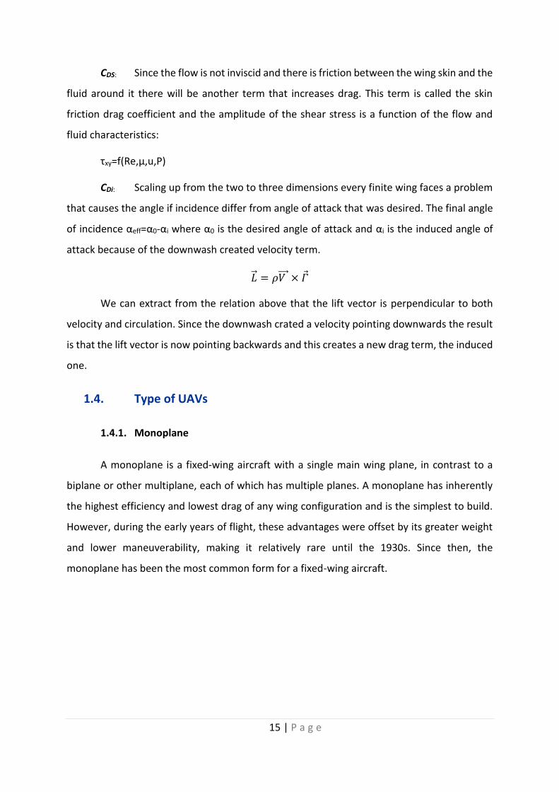
𝐹𝐷 = 𝐶𝐷
𝜌
2𝐴𝑢2
Where CL and CD are respectively the lift and drag coefficients, ρ is the
air density, A the wing area and u the relative airspeed. The CL and CD
heavily depend on the airfoil, the angle of attack and the Reynolds number
Re which is representative of the air flow viscosity.
𝑅𝑒 =𝜌𝑢𝑐
𝜇=
𝑢𝑐
𝜈
Here, μ is the dynamic viscosity that once divided by the air density gives the kinematic
viscosity ν and c represents the chord. The dependency on the angle of attack is depicted in
figure 10. Increasing it makes the CL increase, but progressively the flow separates from the
airfoil starting at the trailing edge and this lets place to a turbulent zone that makes the CD
increase. At stall, the lift is maximum but the drag is high too. After this point, the behavior is
more difficult to predict or simulate, but basically the drag still increases but without being
followed by the lift that drops. Thus, the interesting and safe zone for an airplane is before the
stall point, for glider especially at the point where the glide ratio CL/CD is maximum.

14 | P a g e
Figure 1-11: Lift and drag coefficients depending on the angle of attack
What was depicted so far is the case of an infinite length wing and inviscid flow but for
a real wing, the total drag is the sum of five components:
C0 is the drag due to pressure difference
CDi is the induced drag that is generated from the wingtip vortex
CDS is the overall shear stress due to friction between the wing and the fluid
CDw is created since the object disturbs the surround fluid and a wave extending from
the wing is generated pushing outwards the surroundings and this change in
momentum is added to the overall drag.
CD0: Visualizing the flow around and object with the help of steam, we can observe
high and low streamline density areas. When the streamlines are closer one to other the fluids
speed is greater than areas with greater distance between the streamlines and from
Bernoulli’s principle we can find out that the first region has lower and the second one greater
than the free stream pressure. The integral of the pressure around the airfoil will give us the
resultant force which is always perpendicular to the mean airfoil camber as shown below. The
projection of this force in an axis parallel to the free stream flow will give us the first term of
the drag force which is caused by this pressure difference between the upper and lower
surface.
15 | P a g e
CDS: Since the flow is not inviscid and there is friction between the wing skin and the
fluid around it there will be another term that increases drag. This term is called the skin
friction drag coefficient and the amplitude of the shear stress is a function of the flow and
fluid characteristics:
τxy=f(Re,μ,u,P)
CDi: Scaling up from the two to three dimensions every finite wing faces a problem
that causes the angle if incidence differ from angle of attack that was desired. The final angle
of incidence αeff=α0-αi where α0 is the desired angle of attack and αi is the induced angle of
attack because of the downwash created velocity term.
�⃗� = 𝜌𝑉 ⃗⃗ ⃗ × 𝛤
We can extract from the relation above that the lift vector is perpendicular to both
velocity and circulation. Since the downwash crated a velocity pointing downwards the result
is that the lift vector is now pointing backwards and this creates a new drag term, the induced
one.
1.4. Type of UAVs
1.4.1. Monoplane
A monoplane is a fixed-wing aircraft with a single main wing plane, in contrast to a
biplane or other multiplane, each of which has multiple planes. A monoplane has inherently
the highest efficiency and lowest drag of any wing configuration and is the simplest to build.
However, during the early years of flight, these advantages were offset by its greater weight
and lower maneuverability, making it relatively rare until the 1930s. Since then, the
monoplane has been the most common form for a fixed-wing aircraft.

16 | P a g e
Figure 1-12: VTOL Vehicles
1.4.2. VTOL Vehicles
A vertical take-off and landing (VTOL) aircraft is one that can hover, take off, and land
vertically. This classification can include a variety of types of aircraft including fixed-wing
aircraft as well as helicopters and other aircraft with powered rotors, such as cyclogyros/
cyclocopters and tiltrotors.
Figure 1-13: VTOL Fixed Wing UAV
1.4.3. Multicopters
A multicopter is a rotorcraft with more than two rotors. An advantage of multirotor
aircraft is the simpler rotor mechanics required for flight control. Unlike single and double-
rotor helicopters which use complex variable pitch rotors whose pitch varies as the blade

17 | P a g e
rotates for flight stability and control, multirotors often use fixed-pitch blades. Control of
vehicle motion is achieved by varying the relative speed of each rotor to change the thrust
and torque produced by each.
Due to their ease of both construction and control, multirotor aircraft are frequently
used in radio control aircraft and UAV projects in which the names tricopter, quadcopter,
hexacopter and octocopter are frequently used to refer to 3-, 4-, 6- and 8-rotor rotorcraft,
respectively.
Figure 1-15: Tricopter Figure 1-14: Quadcopter
Figure 1-17: Hexacopter Figure 1-16: Octocopter

18 | P a g e
Figure 2-1: Solar Irradiance
Chapter2: Preliminary Analysis
The monoplane selection for the purpose of our application give us plenty of room for
tuning and modification in the geometry while still maintaining a very simplistic and delicate
way of achieving our goal. The greatest advantage among different kinds of aerial vehicles is
the large wing areas that is necessary to exist in order to acquire enough irradiation from the
sun for the whole system to function in the desired point. At this point we need to do some
preliminary calculation and analysis in order to acquire the desired goals for the aerodynamic
coefficients and the area need for the solar energy gathering.
2.1 Solar Irradiance in Greece
The irradiance depends on a lot of variables such as geographic location, time, plane
orientation, weather conditions and albedo that represents the reflection on the ground
surface. A typical diagram of solar irradiation during day can be seen below. The interpolated
data can be then integrated and acquire either the average amount of irradiation or the total
amount of irradiance that is emitted over an area. Our goal here is to use some average values
and see weather our solar powered UAV can be used throughout the year or if it is restricted
from weather conditions during winter season. Radiation data for the city of Volos show that
the irradiation ranges from 1.93 kWh/m2/day up to 6.85 kWh/m2/day which corresponds to
80 and 285 W/m2 respectively.
19 | P a g e
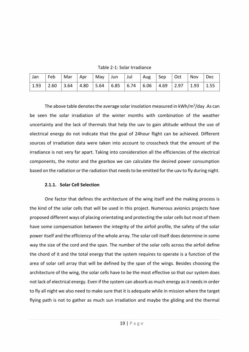
Table 2-1: Solar Irradiance
The above table denotes the average solar insolation measured in kWh/m2/day .As can
be seen the solar irradiation of the winter months with combination of the weather
uncertainty and the lack of thermals that help the uav to gain altitude without the use of
electrical energy do not indicate that the goal of 24hour flight can be achieved. Different
sources of irradiation data were taken into account to crosscheck that the amount of the
irradiance is not very far apart. Taking into consideration all the efficiencies of the electrical
components, the motor and the gearbox we can calculate the desired power consumption
based on the radiation or the radiation that needs to be emitted for the uav to fly during night.
2.1.1. Solar Cell Selection
One factor that defines the architecture of the wing itself and the making process is
the kind of the solar cells that will be used in this project. Numerous avionics projects have
proposed different ways of placing orientating and protecting the solar cells but most of them
have some compensation between the integrity of the airfoil profile, the safety of the solar
power itself and the efficiency of the whole array. The solar cell itself does determine in some
way the size of the cord and the span. The number of the solar cells across the airfoil define
the chord of it and the total energy that the system requires to operate is a function of the
area of solar cell array that will be defined by the span of the wings. Besides choosing the
architecture of the wing, the solar cells have to be the most effective so that our system does
not lack of electrical energy. Even if the system can absorb as much energy as it needs in order
to fly all night we also need to make sure that it is adequate while in mission where the target
flying path is not to gather as much sun irradiation and maybe the gliding and the thermal
Jan Feb Mar Apr May Jun Jul Aug Sep Oct Nov Dec
1.93 2.60 3.64 4.80 5.64 6.85 6.74 6.06 4.69 2.97 1.93 1.55
20 | P a g e
chasing process will be replaced by the desired mission. That said we can understand that
there is no room for efficiency losses in the selection of the panels.
One mounting technique which is not very efficient is to take small rectangular
stiff panels and stick them on the upper side of the wing. The benefit of this method is that
the small area of each panel allows to cover even the tiniest gaps in the whole glider, and they
play not a very important role in the wing dimensions. They can even cover the moving control
areas like ailerons rudders etc without adding much weight. The major disadvantage of those
cells is that the airfoil should not have great gradients in its geometry because the cells in
order to be placed they will remove the curvature altering the whole geometry. One can think
of it as integrating a continuous function with the trapezoid method. The final shape of the
wing will be way different from the designed one and all the minor edges on the wing can
cause early flow separation and thus decreasing the efficiency of the uav. This method was
used as an initial concept in sunsailor (Israel 2006).
The second mounting technique is the safest for the solar cells themselves
because they are encapsulated inside the wing and mounted on the spars and ribs of it. This
method preceds that the architecture of the wing will not be made by composite materials as
we plan but with some spar and rib grid and that the upper skin of the glider will be made by
a transparent material. That way the cells may be very well protected by the surrounding wing
but there are some serious disadvantages that make them unwanted for our purposes. First
of all the spar and rib architecture is a pretty complicated structure that needs further study
in order to get the desired stiffness of the wing. It can also result in a very bulky heavy and
compact assembly without sufficient space for extra electronics after the manufacturing
process. The encapsulation of the solar cells comes with the insufficient head disposal
increasing the temperature inside the wing and thus decreasing the effectiveness of all the
electronic components. But again the major disadvantage is that the geometry of the upper
wing skin has to be made by a transparent material which in most cases is of a membrane
type. The membrane might have adequate rigidity to endure hard maneuvering and
temperatures but some of the irradiance will be reflected from the surface and they cannot
guarantee that the geometry of the wing will remain as was designed.

21 | P a g e
Figure 2-2: Encapsulated Solar Cells
The third and base on the above thoughts concept is to use flexible solar panels. As
their name indicates the solar panels are flexible up to 45 degrees and their efficiency rises up
to 24% which is one of the most efficient solar panel that exists today. They have rectangular
shape with 12.5 mm side and as all the solar cells they can be connected serial or parallel
based on the current and the voltage required. They can be mounted on the outter surface of
the wings not effecting the manufacturing process and since they are flexible they can enfold
the wing. They are only 0.3 mm thick and there is no need to create a slot in the wing in order
to keep the curvature of the wing intact. As for the thermal behavior the placement in the
outer surface of the construction will provide the desired cooling.

22 | P a g e
The selection was very clear and without doubts. The Maxeon Gen II left no space for
controversies for the type of the solar cell that will be used as well as for the type of the
manufacturing process of the UAV. The composite combined with the foam is a robust
material selection we previous validation in a race car aerodynamics package and the
existence of the flexible solar panel allows us to use this method to incarnate our project.
2.2. UAV Type Selection
In chapter one we did present some of the aerial vehicles that exist today and some of
them might be appropriate for surveillance but very few can be capable to succeed the 24-
hour flight endurance time. All the multicopters and VTOL airplanes do have the advantage of
the easiest control among the others but their power consumption exceeds our limitations.
Figure 2-3: Flexible Solar Cells
Figure 2-4: Maxeon Gen II

23 | P a g e
Their major issue is that their shape consists of very small area for solar cell placement and
even if they do the model becomes bulky and stiff and in most cases aesthetically poor. The
ideal airplane shape is the monoplane because of its simplistic shape and the relative big area
to weight ratio, it can be light weight and can absorb the amount of energy that we require.
The other advantage of the monoplane is that the simplistic shape of it is that once knowing
the airfoil profile there are only two variables do be defined, the chord and the span of the
wing. Since we do need to place some cells on the outer surface we can understand that the
chord cannot be arbitrary but it should have adequate space for the panels to be placed. Thus
the chord has to be at least 12.5 cm times the rows of the solar cells that will be placed. In
example one row of cells will result in a very long wing which is not desired because of the
stress concentration in the base of the wing and a huge amount of cell rows will result in a
very short wing and as we did present in the first chapter the smallest the aspect ratio the
lower the efficiency of the wing. The answer will be found somewhere in the middle but we
need do take into consideration that the airfoil profile should not have great gradients for the
cells to be placed, to be placed in a small angle of attack for the greater sun irradiance
absorbance and the chord of the wing will be such that the efficiency is great enough end the
stresses can be handled by the composite material.
2.3. Initial Sizing
The initial sizing method that is introduced in Snori Gudmundson General Aviation Airc
is based on preliminary calculations and is based on thrust to weight ratio to define
parameters of the UAV such us stall speed maximum lift coefficient cruising speed and then
calculate based on standard tables the wing area of the airplane. Since we do not have yet
chose an appropriate motor and propeller we need to find an alternative way to calculate the
properties of the wing that we need. Furthermore, our analysis will be based on the level flight
and will ignore the take off and the landing of the aerial vehicle. The initial calculations of the
power consumption and the efficiencies of the electronics were taken from similar projects.
The power needed is calculated as:
𝑃𝑜𝑢𝑡 = 𝑛𝑝𝑟𝑜𝑝𝑒𝑙𝑙𝑒𝑟𝑛𝑟𝑒𝑑𝑢𝑐𝑒𝑟𝑛𝑀𝑃𝑃𝑇𝑛𝑒𝑙𝑒𝑐𝑡𝑟𝑜𝑛𝑖𝑐𝑠𝑛𝑠𝑜𝑙𝑎𝑟_𝑐𝑒𝑙𝑙𝑠 ∗ 𝑠𝑢𝑛_𝑖𝑟𝑟𝑎𝑑𝑖𝑎𝑡𝑖𝑜𝑛

24 | P a g e
Table 2-2: Electronics' efficiencies
Npropeller Nreducer Nmppt Nelectronics Nsolar_cells
0.85 0.95 0.97 0.93 0.24
Based on the irradiation data in Volos during the summer season the amount of daily
irradiation is 250watt/m2. For that irradiation power the Pout is equal to 46.0071 watt/m2.
This means that for a wing area of one square meter we need to have a drag power
consumption of around 23 watts in order for the rest of the power to be stored in the batteries
and used overnight. As Snori gundmundson indicates typical drag coefficient values for high
efficiency devices are between 0.04-0.05 for Gliders and typical cruising speeds are around 10
m/s. So for those two values taking the worst scenario of the uav Cd coefficient which is 0.05
we can calculate the initial Area of the wing.
𝑃𝑑𝑟𝑎𝑔 =1
2𝜌𝐶𝐷𝐴𝑢3 ⇔
46 =1
2∗ 1 ∗ 0.05 ∗ 103𝐴 ⇔
𝐴 = 1.84 𝑚2
We can round the area of the wing in 1.9m2 making things more strict in order of drag
power. So now that we do have the area of the wing we need to define the chord of it. As said
before we need to have adequate space for the cells to be placed on it. The two concepts of
placing one and three rows of cells are have disadvantages the first one in the margin of the
stresses and the second one in the efficiency of the wing. Thus placing two series of panels
will result in a chord that is more or less, greater than 25 centimeters. Considering that we
need space for the ailerons and the leading edge section that the panels cannot be placed due
to the tilt of them we can say that a sufficient chord will be in around 30 centimeters. The
planform area of the wing is 1.84m2 and with a 0.3 m chord the span of the wings will be
6meters long. All the above calculations are based on speeds that gliders fly and data that

25 | P a g e
were taken in literature. During the design process those dimensions are very likely to be
altered to match our criteria.
2.3.1. Lifting Line Theory(LLT)
Based on Jan (Lan, 1997) who quotes Prandtl’s the lifting line theory as a bridge to
connect the 2D airfoil Cl and Cd coefficients with the 3D wing parameters we can have an
expression of the wing aerodynamic coefficients with a very simply way just by using an Excel
Sheet. As he denotes
From the Momentum Method:
According to the linear momentum principle, assuming uniform downwash over the
span of the wing S’:
𝐿 = 𝜌𝑉(𝑆′𝑉)𝑤1
𝑉= 𝜌𝑤1(𝑆
′𝑉)
And from the Energy Method which relies that
The work done on the air mass per unit time equals the kinetic energy increase
per unit time.
Therfore :
𝐷𝑖𝑉 = 𝜌𝑆′𝑉𝑤1
2
2
Dividing by V yields:
𝐷𝑖𝑉 = 𝜌𝑆′𝑤1
2
2
Recalling Eqn:
𝐿 =𝐷𝑖
𝑎𝑖=
𝜌𝑆′𝑤1
2
2𝑤𝑉
From this it follows that:
𝜌𝑤1(𝑆′𝑉) = 𝜌𝑆′
𝑉𝑤12
2𝑤

26 | P a g e
From this, it is now seen that:
2𝑤 = 𝑤1
This result means that the induced downwash far behind the wing is twice that of the
downwash on the wing itself. The area, S’ may be written as: 𝑆′ =𝜋𝑏2
4. Thus, it is seen that the
equation may be written as:
𝐿 = 𝜌(2𝑤)𝜋𝑏2
4𝑉
This is just another way of writing previous equation. Now solving for the downwash,
w:
𝑤 =2𝐿
𝜌𝜋𝑏𝑉2=
𝐶𝐿𝑞𝑆𝑉
𝜋𝑞𝑏2=
𝐶𝐿𝑆𝑉
𝜋𝑏2=
𝐶𝐿𝑉
𝜋𝛢
The angle, αι may now be written as:
𝛼𝑖 =𝑤
𝑉=
𝐶𝐿
𝜋𝛢
Also, it follows that:
𝐷𝑖 = 𝐿𝑎𝑖 = 𝐶𝐿𝑞𝑆𝐶𝐿
𝜋𝛢
The induced drag coefficient can therefore be written as:
𝐶𝐷𝑖=
𝐷𝑖
𝑞𝑆=
𝐶𝐿2
𝜋𝛢
These equations are only valid for wings with uniform downwash distribution.
The latter can be achieved only if the span loading of the wing is elliptical. It has been shown
that in such a case the induced drag coefficient is a minimum. It is shown as Jan Roskam implies
that this condition can be achieved using an elliptical planform. When, as is normally the case,
the downwash distribution is not uniform, a correction factor “e” called Oswald efficiency
factor is introduced to yield:
𝐶𝐷𝑖=
𝐶𝐿2
𝜋𝛢𝑒
Therefore, the induced angle, αi can be written as:
𝛼𝑖 =𝐶𝐿
𝜋𝛢𝑒
Experimentally it has been found that e ranges from 0.85 to 0.95 for a wind by itself.
27 | P a g e
The factor Ae is frequently referred to as the effective aspect ratio: Aeff. The
total drag coefficient for a wing can therefore be written as:
𝐶𝐷 = 𝐶𝐷0+
𝐶𝐿2
𝜋𝛢𝑒𝑓𝑓
Where: 𝐶𝐷0 is the lift independent sum of skin friction and pressure drag.
The factor Ae can be used to determine the lift curve slope of one wing from
knowledge of the lift curve slope of another wing. To show this, assume that two wings have
high but different aspect ratios. Also assume that both wings use the same airfoil. According
to Prandtl’s Lifting Line Theory if these wings are placed at the same effective angle of attack,
αa=α-α0 , their lift coefficient, CL will be the same. The angle αa=α-α0 is called the absolute
angle of attack and a0 is the angle of attack for zero lift. Therefore:
𝑎𝑎1−
𝐶𝐿
𝜋(𝐴𝑒)1= 𝑎𝑎2
−𝐶𝐿
𝜋(𝐴𝑒)2
𝛼𝑎1= 𝛼𝑎2
+𝐶𝐿
𝜋{
1
(𝐴𝑒)1−
1
(𝐴𝑒)2}
Because the lift curve slope, a, is related to the lift coefficient by:a
𝐶𝐿 = 𝑎𝑎𝑎
It follows that:
𝐶𝐿
𝑎1=
𝐶𝐿
𝑎2+
𝐶𝐿
𝜋{
1
(𝐴𝑒)1−
1
(𝐴𝑒)2}
From the latter the lift curve slope of one wing follows from that for the other wing
from:
𝑎1 =𝑎2
1 +𝑎2
𝜋 {1
(𝐴𝑒)1−
1(𝐴𝑒)2
}
Again, this equation allows an estimate of the lift curve slope, a1 of one wing
with effective aspect ratio, (Ae)1 if the corresponding, but different, properties of the other
wing are known. This result should be used only for high aspect ratio wings. Generally, for A>5
the relation works well. The previously shown figure shows the effect of aspect ratio of wings
with the same angle of attack for zero lift. Note that wings of varying aspect ratio tend to have
28 | P a g e
approximately the same angle of attack for zero lift. The lift curve slope is seen to decrease
significantly with increasing aspect ratio. That effect agrees with Eqn (4.30).
For the same wing area and for the same airfoils, the wing zero lift drag is also
essentially independent of aspect ratio. Application of induced drag equation to two wings
which differ only in aspect ratio yields:
𝐶𝐷𝑖= 𝐶𝐷2
+𝐶𝐿
2
𝜋{
1
(𝐴𝑒)1−
1
(𝐴𝑒)2}
The drag polars show that, although the drag coefficients at zero lift are
essentially independent of aspect ratio marked reductions in the drag coefficient CD, occur as
the aspect ratio is increased. This is particularly true at high values of lift coefficient, CL.
Equations 4.27 and 4.31 can be used to reduce the data to a wing with a
common aspect ratio. It can therefore be concluding, that the characteristics of a wing of one
aspect ratio may be predicted with considerable accuracy from similar data on a wing of
different aspect ratio.
Eqn(4.30) can be used to determine the lift curve slope of a wing 1 when the
characteristics of a wing 2 with the same airfoil section are known. If wing 2 has an infinite
aspect ratio (i.e. is the equivalent of a two-dimensional airfoil selection), Eqn (4.30) can be
reduced to:
𝑎1 =𝑎∞
1 +𝑎∞
𝜋𝛢𝑒
As it was previously mentioned the above equation produces good results only
for wins with aspect ratios larger than 5 and with sweep angles below about 15 degrees. In
our case the UAV will not utilize the sweep angle and so the above assumption can take place.
We can now use the above methodology to estimate the lift and the drag of a
planform wing with arbitrary profile of airfoil used in it. Thus we can obtain. The two
dimensional data the xflr5 simulations to get a first estimation of the plane characteristics.
The first option is to take the slope of the Cl vs AoA curve of the airfoil, interpolate them
integrate the polynomial equation and use the zero lift angle of attack value as a condition to
calculate the integration constant, or we can either begin from the zero lift angle of attack and
since we know the slope of the curve we can apply a shooting method (Taylor series with one
term for example), to find the value of the lift at the next point. From the next point we again
know the slope of the curve and by ‘shooting’ again we obtain the Cl of the new angle of attack
and so on until we reach the angle of attack that we desire. In our case we used the second
method with only one term in the Taylor series also known as Euler’s method for solving first
order differential equations with increment of one degree. It is also important to mention that
if we chose to calculate the Cl in more than 15 points the first method has a tremendous

29 | P a g e
disadvantage because high order polynomials tend to oscillate between the interpolation
values and thus either some Spline method should be used or break the whole domain in
smaller spaces and apply the polynomial interpolation in sections.
2.3.2. High Lift Devices
We can say that an airfoil is a device that can generate enough lift force with relatively
small generation of drag otherwise it can be called a bluff body. The airfoil pool that we are
interested in is the high efficiency ones which means that the ratio of the Cl to Cd ratio is
relatively higher from other airfoils and this means that they can generate the same amount
of lift while producing less drag. A family of this kind of airfoils and the most common and
widely use onces are the NACA 4-digit and NACA-5digit. Although that NACA airfoils tend to
have a very consistent behavior in different Reynolds numbers and maintain a high efficiency
we will not use them as a main wing airfoil but we will only use a symmetrical one as control
surface in the empennage of the glider. Most of the airfoil coordinates that we collected can
be found online via the site http://airfoiltools.com/ . The diagrams for the airfoil’s behavior
are extracted by using the XFLR tool. The following table summarizes the airfoil name the
application that they were designed for, the projects that they were used at and some
geometrical parameters such as maximum airfoil thickness, foil perimeter and the cross area
of them. These specs will later on be used on the weight estimation method and also as criteria
for airfoil rejection. The pool consists of 31 airfoils with the NACA0012 not included because
it won’t be used as a lift device but as a control surface
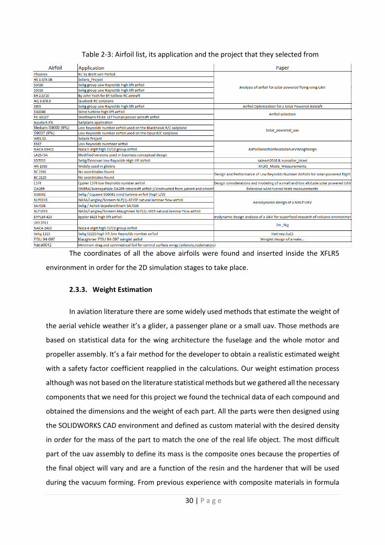
30 | P a g e
Table 2-3: Airfoil list, its application and the project that they selected from
The coordinates of all the above airfoils were found and inserted inside the XFLR5
environment in order for the 2D simulation stages to take place.
2.3.3. Weight Estimation
In aviation literature there are some widely used methods that estimate the weight of
the aerial vehicle weather it’s a glider, a passenger plane or a small uav. Those methods are
based on statistical data for the wing architecture the fuselage and the whole motor and
propeller assembly. It’s a fair method for the developer to obtain a realistic estimated weight
with a safety factor coefficient reapplied in the calculations. Our weight estimation process
although was not based on the literature statistical methods but we gathered all the necessary
components that we need for this project we found the technical data of each compound and
obtained the dimensions and the weight of each part. All the parts were then designed using
the SOLIDWORKS CAD environment and defined as custom material with the desired density
in order for the mass of the part to match the one of the real life object. The most difficult
part of the uav assembly to define its mass is the composite ones because the properties of
the final object will vary and are a function of the resin and the hardener that will be used
during the vacuum forming. From previous experience with composite materials in formula

31 | P a g e
student wing manufacturing process, we can estimate the amount of the carbon fiber mass
that will be used as well as the carbon to resign ratio and the overall volume of the
polyurethane foam that will be used inside the wings.
For the estimation of the total mass we considered taking the worst case scenario. The
heaviest part of the wing and fuselage part is the resign and the carbon fiber cloth. The foams
that will be used have density around 30kg/m3 and thus we can tell that their contribution to
the whole glider mass is not of vital importance. That said the weight of a wing with
rectangular top view can be acquired as:
𝑚𝑡𝑜𝑡𝑎𝑙 = 𝑚𝑐𝑎𝑟𝑏𝑜𝑛 + 𝑚𝑝𝑜𝑙𝑢𝑜𝑢𝑟𝑒𝑡ℎ𝑎𝑛𝑒
Or
𝑚𝑡𝑜𝑡𝑎𝑙 = 𝐴𝑐𝑎𝑟𝑏𝑜𝑛 ∗𝐶𝑎𝑟𝑏𝑜𝑛𝑚𝑎𝑠𝑠
𝐴𝑟𝑒𝑎+ 𝐴𝑓𝑜𝑖𝑙 ∗ 𝑏 ∗ 𝜌𝑓𝑜𝑎𝑚
Where Afoil is the area of the chosen airfoil, b is the span of the wing and ρfoam is the
density of the foam. As was discussed previously the carbon mass is the greater one because
it includes the mass of the resin with a 0.4 carbon to resign ratio. Thus to acquire the worst
case scenario we did calculate the perimeter of all the airfoils and then we calculated the mass
of the wing that uses the corresponding foil as profile. The results of the structural mass
prediction are shown in the table below:

32 | P a g e
Table 2-4: Structural weight estimation
Besides the mass of the structural components, we also need to take into
consideration the mass of the electrical parts that will be used in this project and even add a
payload mass that may be added in the future. Because of the amount of the batteries that
we need to use in order for the glider to endure a whole night flight the total weight of the
electrical components pay a very serious role in the overall process. We did thought neglect
the contribution of wires, tie wraps spacers etc.
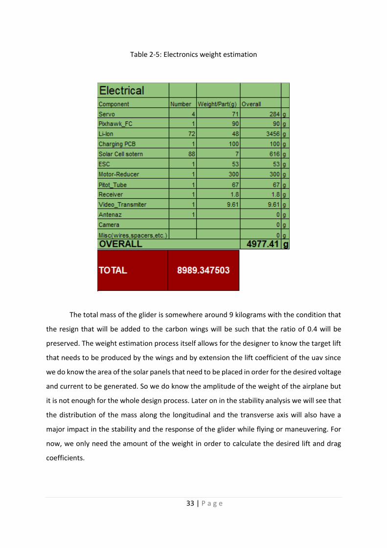
33 | P a g e
Table 2-5: Electronics weight estimation
The total mass of the glider is somewhere around 9 kilograms with the condition that
the resign that will be added to the carbon wings will be such that the ratio of 0.4 will be
preserved. The weight estimation process itself allows for the designer to know the target lift
that needs to be produced by the wings and by extension the lift coefficient of the uav since
we do know the area of the solar panels that need to be placed in order for the desired voltage
and current to be generated. So we do know the amplitude of the weight of the airplane but
it is not enough for the whole design process. Later on in the stability analysis we will see that
the distribution of the mass along the longitudinal and the transverse axis will also have a
major impact in the stability and the response of the glider while flying or maneuvering. For
now, we only need the amount of the weight in order to calculate the desired lift and drag
coefficients.

34 | P a g e
Chapter3: 2D Analysis
As was previously discussed the LLT is a method that can allow us to save time by
running 2D simulations and then, since our wing has an Aspect ratio of 20, map the existing
results to a planform wing that was created by extruding the profile of the airfoil. The above
simulation took place in XFLR5 environment and there is the capability of batch analysis which
means that the user gives as input the desired range of angles of attack and Reynolds number
and the simulations take place one after another.
3.1. 2D simulations
The 2D XFLR5 simulation environment solves the Euler’s equations which arise from
the Navier-Stokes equation with the assumption of inviscid and irrational flow around the 2D
airfoil. The above assumptions can give some good results only in cases where the Reynolds
number is high enough and the viscous term of the drag is negligible. In other words, the
farther we are from the creeping flow the more precise the results that we will acquire. Those
two assumptions come along with the Kutta condition in the trailing edge of the airfoil. The
Kutta condition indicates that in an inviscid flow the speed of the fluid in the upper and the
lower side of the airfoil match at the trailing edge and the wake remains calm and undisturbed.
Figure 3-1: Kutta's condition

35 | P a g e
The examination of the steady flight of the uav in the altitude of 2000 meters
has as a result the atmospheric pressure to drop around 78.000 Pa and the density of the air
to decrease around 10 percent which means that at that altitude is equal to 1. Along with the
density the viscosity of the air has also decreased and reached 17.84E-06 Pa*s. It will be later
on used on the 3D simulation with the VLM method. The Reynolds number is calculated at
that speed and altitude and is equal to Re=250.000 and the corresponding Mach number is
Ma=0.036 which is far away from the 0.3 area where the flow is considered compressible. That
said we used the batch analysis method and run calculations for each airfoil from -5 up to 15
degrees Angle of Attack in order to capture the zero lift angle of attack for the 3D wing
estimation process. All the airfoil results had the form that we did expect with some having
better efficiency over others.
Figure 3-2: XFLR5 2d simulation Laplace Equation
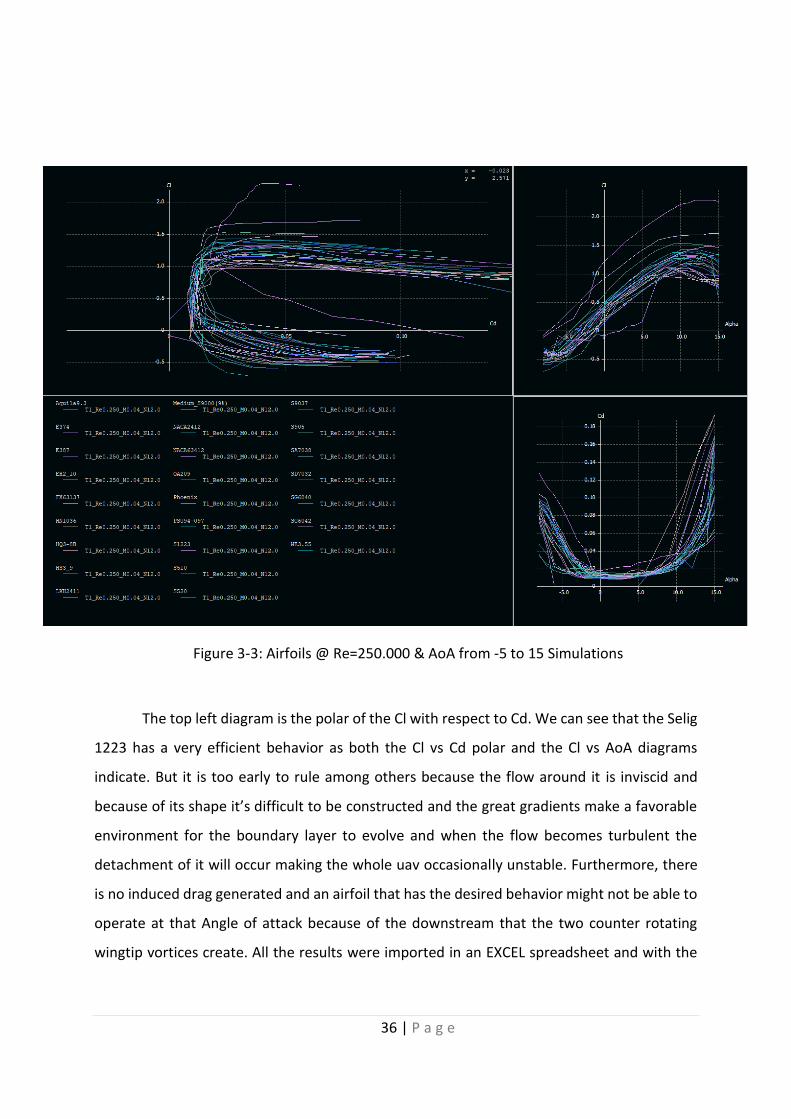
36 | P a g e
The top left diagram is the polar of the Cl with respect to Cd. We can see that the Selig
1223 has a very efficient behavior as both the Cl vs Cd polar and the Cl vs AoA diagrams
indicate. But it is too early to rule among others because the flow around it is inviscid and
because of its shape it’s difficult to be constructed and the great gradients make a favorable
environment for the boundary layer to evolve and when the flow becomes turbulent the
detachment of it will occur making the whole uav occasionally unstable. Furthermore, there
is no induced drag generated and an airfoil that has the desired behavior might not be able to
operate at that Angle of attack because of the downstream that the two counter rotating
wingtip vortices create. All the results were imported in an EXCEL spreadsheet and with the
Figure 3-3: Airfoils @ Re=250.000 & AoA from -5 to 15 Simulations

37 | P a g e
use of the previous methodology that was developed and by using Taylor Series with only one
term the 3D Cl and Cd data were calculated for all the above operation points.
3.2. Selection Criteria and 2D Airfoil Comparison
Once the initial size of the whole airplane was defined and the preliminary dimensions
of the wing we had to choose among a wide variety of airfoils and wing types. We came across
with 30 different airfoils each of one is considered either high performance or high lift device
in low Reynolds number flights. At first we did utilize the XFLR5 environment for the majority
of the cases, because of the ease and the short simulation time of it. In avionics projects
phenomena such us wing flutter and wind fluctuations, boundary layer detachment and
reattachment, the effects of the roughness of the wing surface, compressibility effects,
propeller wake etc. that can alter the nature of the flight and that transient simulation have
to take place in order for a better understanding and design of the glider. However, our thesis
does not extend to that level and a steady state simulation is used in all cases for comparison.
So our first goal is to reject the majority of the airfoils and pick those that have the better
performance. So we did set some strict criteria in order to start restricting our choices. Thus
the criteria that were set focus on the aerodynamic performance of the wing and in
miscellaneous factors that can affect our glider. Most popular and of main importance are the
following:
High 𝐶𝑙
𝐶𝑑 ratio
Lift distribution within the desired flight range (constant function of velocity is preferable)
Maximum thickness for structural installation with batteries encapsulation in the wing
High 𝐶𝑙
32
𝐶𝑑 ratio. This is a term that was extracted for maximum endurance- minimum power
consumption
Adequate lift in moderate angles of attack for high solar irradiation absorbance
Low Cm amplitude for minimum torsional stress concentration at the fuselage-wing
connection
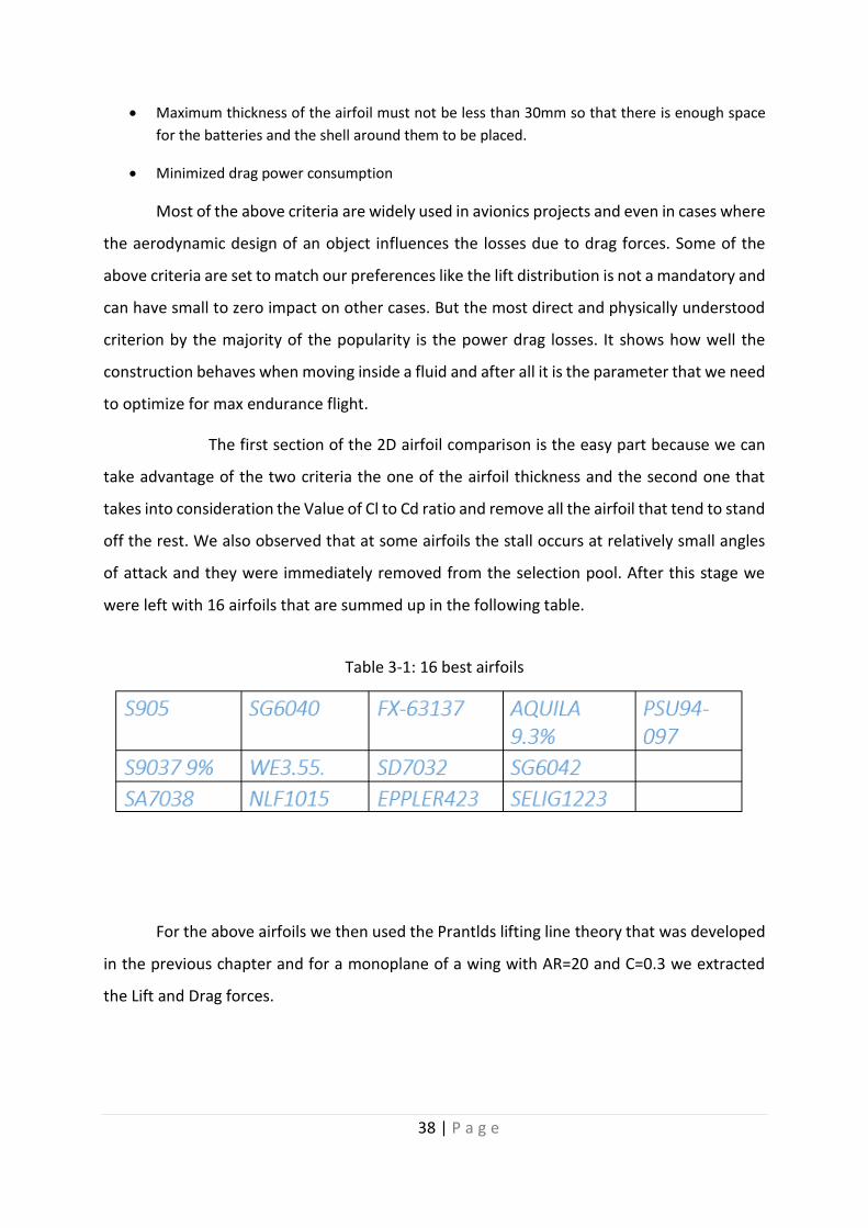
38 | P a g e
Table 3-1: 16 best airfoils
Maximum thickness of the airfoil must not be less than 30mm so that there is enough space
for the batteries and the shell around them to be placed.
Minimized drag power consumption
Most of the above criteria are widely used in avionics projects and even in cases where
the aerodynamic design of an object influences the losses due to drag forces. Some of the
above criteria are set to match our preferences like the lift distribution is not a mandatory and
can have small to zero impact on other cases. But the most direct and physically understood
criterion by the majority of the popularity is the power drag losses. It shows how well the
construction behaves when moving inside a fluid and after all it is the parameter that we need
to optimize for max endurance flight.
The first section of the 2D airfoil comparison is the easy part because we can
take advantage of the two criteria the one of the airfoil thickness and the second one that
takes into consideration the Value of Cl to Cd ratio and remove all the airfoil that tend to stand
off the rest. We also observed that at some airfoils the stall occurs at relatively small angles
of attack and they were immediately removed from the selection pool. After this stage we
were left with 16 airfoils that are summed up in the following table.
For the above airfoils we then used the Prantlds lifting line theory that was developed
in the previous chapter and for a monoplane of a wing with AR=20 and C=0.3 we extracted
the Lift and Drag forces.

39 | P a g e
Table 3-2 :Phoenix XFLR Data
3.2.1. 2D to 3D Estimation
The simulation in the XFLR5 were using nondimensionalization hence the airfoil had
length equal to 1. This means that the match of the 3D data will happen by using the Drag
calculation formula and the area of the wing with the fixed aspect ratio will give us the final
pressure drag and lift. Now we do have the resulting Cl of the two dimensional airfoil from
the XFLR simulations with increment one degree. We did not keep all the values from -5 up to
15 degrees but we reduced that range so that the data of each airfoil include the zero lift angle
of attack.
The previous table is an example of what a spreadsheet of an airfoil looks like after the
data have been imported inside excel. We can tell that the data include the zero Cl angle of
attack since the Cl starts from negative values and then they rise above zero. The zero lift
angle of attack was calculating with linear interpolation of the values prior and after it. The
second stage is to calculate the rate of change of the Cl with respect to the angle of attack. To
do so we used the discretized derivative and the slopes were calculated as

40 | P a g e
𝑑𝐶𝑙
𝑑𝑎=
𝐶𝑙𝑖+1 − 𝐶𝑙𝑖𝑎𝑖+1 − 𝑎𝑖
For i ranging from 0 to the n-1 value of Cl. Then the relation that was extracted from
the Lifting line theory in chapter 2 94.30) can help us to calculate the Cl curve slope of the
corresponding rectangular wing.
𝑎1 =𝑎∞
1 +𝑎∞
𝜋𝛢𝑒
Where a1 is the slope of the wing and a∞ is the slope of the airfoil. Here the e term is
the Oswald efficiency factor and it is equal to 1 for the elliptic lift distribution. The K column
in the excel worksheet uses the above formula to calculate the slope and then with Eulers
method we calculated the L column which has the 3D wing Cl slope. We can see that in the
Phoenix and then in the column M finally the Cl of the wing is found. The above methodology
allows us also to calculate the pressure difference drag and the induced drag but since the
flow is inviscid the friction drag term is neglected. The estimation of the 3D wing Cd is used to
compare the airfoils based on the efficiency criteria. As we know the Reynolds number of our
wing is pretty low and the friction drag cannot be neglected but at this point since the airfoils
have not great gradients on them and the flow can be considered laminar we only use the
calculated values for comparison and further reduce the amount of the airfoils in our pool.
After the final airfoil is chosen we will proceed in Ansys CFD simulations using turbulence
models for better results.
3.3. Airfoil Comparison and Rejection Stages
Having reduce the amount of airfoil profiles that we currently have in our hands we
need not to just estimate the lift of a wing with the LLT but we also need to compare our data
with other methods and then validate the results with a real life testing. The next stage in the
rejection process is to take advantage of the imbedded Vortice Lattice Method that the XFLR5
extension has implemented and use them to further compare and then reject the remaining
airfoils. To do so we designed the 13 above wings and we did run simulations with the VLM
method.

41 | P a g e
Figure 3-4: VLM Panels And Circulation Γi
A solution for three-dimensional wings of any general form can be obtained by using a
vortex lattice model. For incompressible, inviscid flow, the wing is modelled as a set of lifting
panels. Each panel will contain a single horse-shoe vortex. A bound vortex is located at the
panel 1/4 chord position with two trailing vortex lines shed from each end.
Both span-wise and chord-wise variation in lift can be modelled as a set of step changes
from one panel to the next.
The required strength of the bound vortex on each panel will need to be calculated by
applying a surface flow boundary condition. The equation used is the usual condition of zero
flow normal to the surface. For each panel the condition is applied at the 3/4 chord position
along the center line of the panel. The normal velocity is made up of a freestream component
and an induced flow component. This induced component is a function of strengths of all
vortex panels on the wing. Thus for each panel an equation can be set up which is a linear
combination of the effects of the strengths of all panels. A matrix of influence coefficients is
created which is multiplied by the vortex strengths and equal to a right hand side vector of
freestream effects.
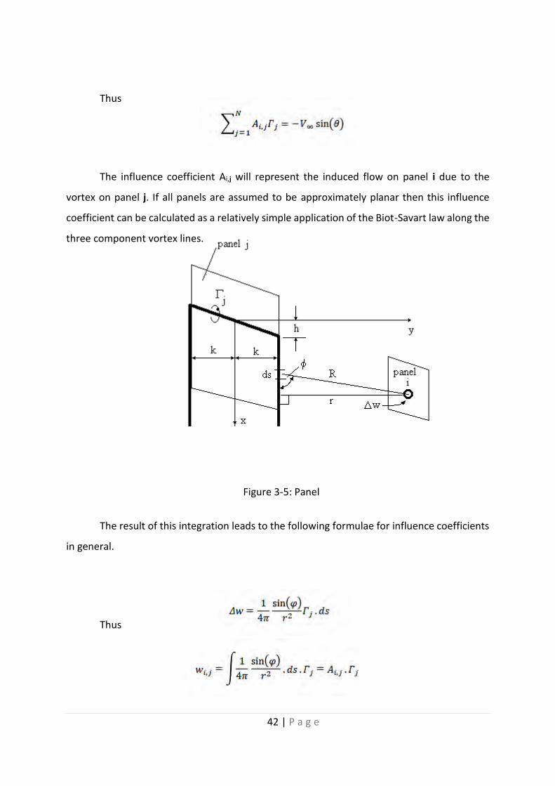
42 | P a g e
Figure 3-5: Panel
Thus
The influence coefficient Ai,j will represent the induced flow on panel i due to the
vortex on panel j. If all panels are assumed to be approximately planar then this influence
coefficient can be calculated as a relatively simple application of the Biot-Savart law along the
three component vortex lines.
The result of this integration leads to the following formulae for influence coefficients
in general.
Thus

43 | P a g e
where the integration is done in three parts, the two trailing lines and the bound
vortex, giving
where
The right-hand side terms for the boundary condition equations will depend upon the
freestream velocity, the angle of attack for the wing and the slope of the panels due to camber
effects.
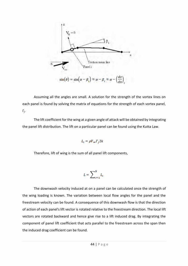
44 | P a g e
Assuming all the angles are small. A solution for the strength of the vortex lines on
each panel is found by solving the matrix of equations for the strength of each vortex panel,
Γj.
The lift coefficient for the wing at a given angle of attack will be obtained by integrating
the panel lift distribution. The lift on a particular panel can be found using the Kutta Law.
Therefore, lift of wing is the sum of all panel lift components,
The downwash velocity induced at on a panel can be calculated once the strength of
the wing loading is known. The variation between local flow angles for the panel and the
freestream velocity can be found. A consequence of this downwash flow is that the direction
of action of each panel's lift vector is rotated relative to the freestream direction. The local lift
vectors are rotated backward and hence give rise to a lift induced drag. By integrating the
component of panel lift coefficient that acts parallel to the freestream across the span then
the induced drag coefficient can be found.

45 | P a g e
Which is the induced drag from panel i.
Therefore, the lift induced drag of the wing is
The induced flow angle (αi≈𝑤𝑖
𝑉∞) represents a rotation of the lift vector backward and
must be calculated from the velocities induced on the bound vortex of the panel by other
panels and the freestream.
Pitching moment about the wing root leading edge can be calculated by summing the
panel lift multiplied by a moment arm which extends in the x-direction from the leading edge
of the wing to the center of the bound vortex for the panel.
At this point a standard wing design procedure would first calculate the Cl and
Cd for a specified Reynolds number or we could better say for a fixed velocity for the angle
range that the wing might fly and repeat the above process until we have data for a desired
velocity range. Then we would calculate based on our weight estimation the stall speed or the
stall angle that the airplane needs to fly in order to maintain a constant altitude and then
compare the above wings and chose the best one. This process is very time consuming and
with the help of XFLR we can choose the option of constant lift generation, which in our case
want to be equal to our weight and then acquire all the stalling velocities of each angle. This
option saves us from multiple simulations and can give us a very clear view of each airfoil
characteristics. With span equal to b=6 meters and chord C=0.3 m we have the above data for
each wing and import them in EXCEL.
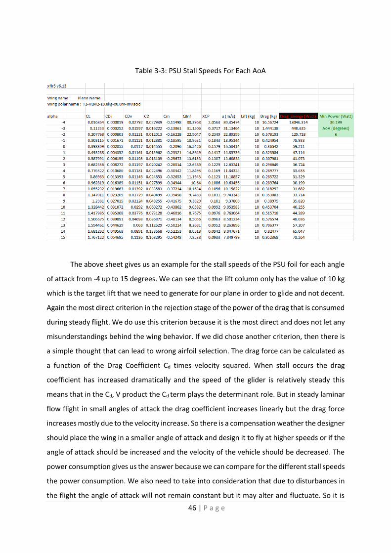
46 | P a g e
Table 3-3: PSU Stall Speeds For Each AoA
The above sheet gives us an example for the stall speeds of the PSU foil for each angle
of attack from -4 up to 15 degrees. We can see that the lift column only has the value of 10 kg
which is the target lift that we need to generate for our plane in order to glide and not decent.
Again the most direct criterion in the rejection stage of the power of the drag that is consumed
during steady flight. We do use this criterion because it is the most direct and does not let any
misunderstandings behind the wing behavior. If we did chose another criterion, then there is
a simple thought that can lead to wrong airfoil selection. The drag force can be calculated as
a function of the Drag Coefficient Cd times velocity squared. When stall occurs the drag
coefficient has increased dramatically and the speed of the glider is relatively steady this
means that in the Cd, V product the Cd term plays the determinant role. But in steady laminar
flow flight in small angles of attack the drag coefficient increases linearly but the drag force
increases mostly due to the velocity increase. So there is a compensation weather the designer
should place the wing in a smaller angle of attack and design it to fly at higher speeds or if the
angle of attack should be increased and the velocity of the vehicle should be decreased. The
power consumption gives us the answer because we can compare for the different stall speeds
the power consumption. We also need to take into consideration that due to disturbances in
the flight the angle of attack will not remain constant but it may alter and fluctuate. So it is

47 | P a g e
important to compare the range of the drag power that will be consumed to get a better
understanding of this phenomenon. We can see that the distribution of the PSU airfoil around
the 6 degrees remains relatively constant. It is a desired behavior for our application and for
application where efficiency is the determinant factor.
After the second stage that was described above we have the pool with the top 10
most efficient airfoils. The selection is not that obvious and for that reason we need to develop
a point gaining system that will split them and will distinguish the best of them. An indicative
value of the behavior of the remaining airfoils can be observed in the diagrams bellow. The
selected airfoils are the 4 best of the pool based on the drag power consumption as was
previously described.
Figure 3-6: Top 4 airfoils

48 | P a g e
Table 3-4: Voting Method
All of the airfoils have the same local minimum value of power consumption which is
30 watts. But we can also observe the behavior of them in greater and smaller angles of attack.
For example, the Wortman airfoil has a pretty constant consumption while the FX increases
rapidly on either side of the local minimum. This behavior is not positive and we do not want
them to act like that unless we can guarantee that the designed operation point will not
change during flight.
The voting method compares the colored cell parameters that are in the second
column and the best of each airfoil is given the lowest number. This means that each airfoil
gathers points based on its performance of each parameter and then the whole column is
added. The airfoil that its points sum is the smallest one is the one that has the better overall
performance. That way we are allowed to compare the airfoils based on the desired criterion.
The star on the Overall row means that the placement has been altered because that airfoils
might have gathered smaller amount of points but the criteria are not the desired. For
example, we did discus that the Cl to Cd ratio might mislead the reader and therefore despite
the fact that the SG6042 airfoil has a smaller sum of points the PSU is the best airfoil since the
Endurance criterion and the minimum power consumption are more important and direct that
the Cl to Cd ratio and therefore the places have been swapped. Another aspect that was not
taken into consideration during the voting process is the distribution that was referred
previously. We can observe that the SG6042 might have better Cl to Cd ratio but the lowest
consumption is not extended for a great range like the PSU.

49 | P a g e
3.4. Experimental Setup
The simulation stage is really important in the design of the UAV but since the XFLR5
is a tool that has not been used in the industry widely and the projects that are designed are
not based to it we cannot claim that the results have the desired precision and besides doing
a further simulation with some turbulence model we designed an experimental setup that will
allow us to validate the results. There was a greater need to compare the 2D simulation results
with a real life testing rather than the 3D wing results. One way of validating is by wind tunnel
testing in the three dimensional wing. Since our university’s wind tunnel cross section area is
not that big we have to scale down the model in order to obtain the Lift of our wing.
Furthermore, drag force calculation demands the existence of a scale measuring method in
the x axis which our University wind tunnel is not designed for this. Our proposition to
calculate only the pressure drag that is generated by an airfoil is to tight fight a wing that has
span equal to the width of the wind tunnel and then measure the static pressure on the upper
and the lower area of the wing using silicon tubes and create a manometer. That said, the
experimental set up consists of :
A 3D printed wing with holes along its chord wise direction. The holes will be created
along its chord for measuring the local static pressure in the upper and lower side.
Silicon tubes that will be used as manometers to measure the static pressure in each
hole.
3D printed adapters that will mount the wing in the side panels of the wind tunnel and
will allow us to change the angle of attack of the wing in the desired range (0-10
degrees).
The two dimensional flow assumption is accurate enough since there will be no gap
between the wind tunnel glass and the wing and so the circulation distribution along the span
of the wing will be the same in each transverse plane. The two major problems that will make
our results deviate from the two dimensional flow is first and foremost the 3d printed wing
surface roughness because it can translate the transition point of the boundary layer further
forward and cause the stall to occur at lower angles of attack and at even higher Reynolds
number as well as the location of the pressure measuring holes because if they are placed

50 | P a g e
close to the wind tunnel wall the development of the boundary layer can alter the acting
pressure over the airfoil. Another aspect to be taken into consideration is the size of the holes,
their number and the alignment. Placing them one really close to another can cause
recirculation of the airflow above them causes the flow that each hole meets be different. In
order to avoid such problems, we will try to avoid placing holes one rear another in the 3d
printed model. Furthermore, the frontal area of objects that will be tested inside a wind tunnel
should not exceed the 5% of the wind tunnel’s cross section area because otherwise the
boundary layer that is created from its walls will affect the flow around the object. In our case
the maximum thickness of our airfoil is 29.5mm and therefore the speed on the upper and
lower area will be increased since the Venturi effect takes place. The speed increase can be
calculated from the continuity equation as:
�̇� =𝜌𝜐𝛢 = 𝑐𝑜𝑛𝑠𝑡𝑎𝑛𝑡
𝜌𝜐1𝛢1=𝜌𝜐2𝛢2
𝑢2 = 𝑢1𝐴1
𝐴2 =𝑢1
𝐻
𝐻−𝑇
Where the H and T are the wind tunnel height and the airfoil maximum thickness
respectively. As a result, the velocity u2 will be:
𝑢2 = 𝑢1700
700−29.5=1.044𝑢1
The design of the wing took place in Solidworks design environment. The wing is
made in parts since the building height of the 3d printer is 165 mm the wing will be made in
5 parts. The middle part will be the one to carry the pressure line holes and will be
connected to the others with press to fit assembly. Each hole is designed to a plane tangent
to the wing surface as shown below:

51 | P a g e
As was shown from the Mathew McCarty’s thesis the hole diameter in pressure
measurement can range from 1.5mm up to 5.4 mm without observing any strange behavior
in the pressure coefficient. The following diagram gives a visual representation of the values
fluctuation which in our case can be considered negligible.
Figure 3-7: Cross Section of the 3D printer Airfoil
Figure 3-8: Hole diameter comparison

52 | P a g e
Once knowing the pressure distribution of an object we can extract the pressure
coefficient (Cp) and by integrating it around it we can obtain the total force that acts on it. As
the figure 2 indicates we need to find the projection of the Lift vector to the perpendicular
direction and then integrate the local Cp to acquire the generated lift.
Thus we can write:
𝐶𝐿 =∫ (𝑝𝑖 − 𝑝∞) sin(𝜃)𝑑𝑠𝐶
12𝜌𝑈∞
2 𝑐
Where θ is the angle of surface normal to free-stream flow. The 15 pressure values
that will be acquired will let us interpolate them and get expressions of the pressure
distribution. It is important to be noted that we have to split the points and create 2 or even
three functions because high order polynomials tend to oscillate between the interpolation
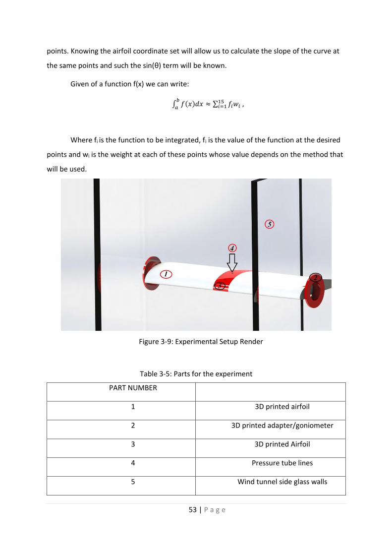
53 | P a g e
points. Knowing the airfoil coordinate set will allow us to calculate the slope of the curve at
the same points and such the sin(θ) term will be known.
Given of a function f(x) we can write:
∫ 𝑓(𝑥)𝑑𝑥𝑏
𝑎≈ ∑ 𝑓𝑖𝑤𝑖
15𝑖=1 ,
Where fi is the function to be integrated, fi is the value of the function at the desired
points and wi is the weight at each of these points whose value depends on the method that
will be used.
Table 3-5: Parts for the experiment
PART NUMBER
1 3D printed airfoil
2 3D printed adapter/goniometer
3 3D printed Airfoil
4 Pressure tube lines
5 Wind tunnel side glass walls
Figure 3-9: Experimental Setup Render

54 | P a g e
The goniometer is 3D printed
and the indications are engraved on
it while still in the printing process. In
case the precision of the angle
measuring is not enough the 3D
printed airfoil can have a specifically
designed slot to enter a Gyroscope.
The adapter is bored so that the
pressure tubes can come outside the
airfoil and end up to the manometer.
The experimental
setup was not performed and was
let as future work.
Figure 3-11: Manometer tube holder
Figure 3-10: 3D printed adapter/goniometer

55 | P a g e
Figure 4-1: Fundamental definitions of a trapezoidal wing planform
Chapter4: Wing
With the end of the 2D simulation process and having validated the results with the
experimental setup that was proposed in the previous section our next step is to define the
parameters of the three dimensional wing and study their effect on the aerodynamic behavior
of our plane.
The above figure represents the fundamental definitions of an arbitrary 3d wing and
all the parameters that can alter its top view shape. Other parameters that cannot be present
by the top view is the dihedral angle and the twist of the wing in the spanwise direction. The
first one plays an important role in the lateral stability around the roll axis as it will be shown
later on the stability section, while the second one is used to decrease the angle of incidence
in the wingtip and by that way decreasing the amplitude of the counter wingtip vortices that
tend to be generated from the pressure difference above and under the wing.
Figure 1 shows the general definitions for the geometry of the trapezoidal planform
and indicates important details of such sections. A leading edge is the part of a lifting surface
that faces the direction of intended movement. The trailing edge is opposite to that side. The
root is the inboard side of the planform and, as can be seen in the figure, is where the two
trapezoids join. This would typically be the centerline of the aircraft or the plane of symmetry.
Although the term root sometimes refers to where the wing intersects the fuselage, that

56 | P a g e
definition is not used in this text because the geometry of the fuselage may be changing and
thus defining a wing chord there would lead to some undesirable issues. The tip is the side
opposite of the root e it is the outboard side. The distance between the left and right tip is
called the span, denoted by the variable b. The transverse dimension is called chord. Thus we
talk about a root-chord or tip-chords the length of the corresponding sides, denoted by the
variables Cr and Ct, respectively. We also call the ratio of the tip-chord to the root-chord the
taper ratio, denoted by l. Another important ratio is the aspect ratio, AR, which indicates the
slenderness of the wing. Both are expressed mathematically below. The quarter-chord line is
drawn from a point one fourth of the distance from the leading edge of the root-chord to a
point one-fourth of the distance from the leading edge of the tip chord. It is important because
two-dimensional aerodynamic data frequently uses the quarter-chord point as a reference
when presenting pitching moment data. Scientific literature, for instance the USAF DATCOM,
regularly uses the quarter-chords a reference point for its graphs and computational
techniques. Additionally, this is often the location of the main spar in lifting surfaces and it is
very convenient to the structural analysts to not have to perform moment transformation
during the design of the structure. The center chord line is obtained in a similar fashion to the
quarter-chord line and is sometimes used as a reference in scientific literature, although not
as frequently. Other important parameters are the sweep angles of the leading edge and
quarter-chord line, denoted by LLE and LC/4, respectively. The mean geometric chord (MGC)
of the planform is often (and erroneously) referred to as the mean aerodynamic chord (MAC),
which is the chord at the location on the planform at which the center of pressure is presumed
to act. The problem is that this location is dependent on three-dimensional influences, such
as that of the airfoils, twist, sweep and other factors, not to mention angle-of-attack, in
particular when flow separation begins. Authors who refer to the MGC as the atypically
acknowledge the shortcoming, present the geometric formulation presented here to calculate
it, before continuing to call it the MAC. In this text, we will break from this convention and
simply call it by its appropriate title e the MGC. The importance of them is that it can be
considered a reference location on a wing, to which the location of the center of gravity is
referenced and even for a quick preliminary estimation of wing bending moments inside it.
Therefore, it is important to also estimate what its span wise station, yMGC, is.

57 | P a g e
Wing Span:
b
Wing Area:
𝑆 = 𝑏(𝐶𝑟 + 𝐶𝑡
2)
Aspect ratio- General:
AR=𝑏2
𝑆
Taper ratio- constant-chord:
𝐴𝑅 =𝑏
𝐶𝑎𝑣𝑔
Taper ratio:
𝜆 =𝐶𝑡
𝐶𝑟
Average chord:
𝐶𝑎𝑣𝑔 =𝐶𝑟 + 𝐶𝑡
2=
𝐶𝑟
2(1 + 𝜆)
Mean geometric chord (MGC):
𝐶𝑀𝐺𝐶 = (2
3)𝐶𝑟(
1 + 𝜆 + 𝜆2
1 + 𝜆)
Mean aerodynamic chord(MAC):
𝐶𝑀𝐴𝐶 ≈ 𝐶𝑀𝐺𝐶
Y-Location of MGCLE:

58 | P a g e
Figure 4-2: Cl vs AoA of a planform wing for different Aspect Ratios
𝑦𝑀𝐺𝐶 = (𝑏
6)(
1 + 2𝜆
1 + 𝜆)
Χ-Location of MGCLE:
𝑥𝑀𝐺𝐶 = 𝑦𝑀𝐺𝐶𝑡𝑎𝑛𝛬𝐿𝐸
Our goal is to define the above parameters so that the final wing setup meets our
criteria. To begin with we have to understand what are the differences of a 3d wing
aerodynamic behavior compared to its foil. The simplest wing that can be generated from an
airfoil is the planform because it has steady chord along its span, has no twist or taper ratio
and overall is an extrusion of the foil to the 3rd dimension. Comparing the lift coefficient of a
2d foil with its planform wing for a constant chord C for different angles of attack we can see
that increasing the span of the wing and such the AR of it the Cl curve tends to increase and
try to match the one of the airfoil as shown in the figure below.
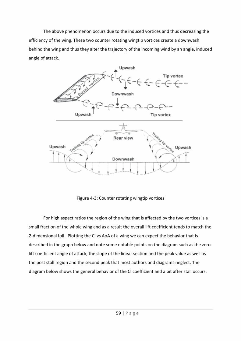
59 | P a g e
The above phenomenon occurs due to the induced vortices and thus decreasing the
efficiency of the wing. These two counter rotating wingtip vortices create a downwash
behind the wing and thus they alter the trajectory of the incoming wind by an angle, induced
angle of attack.
For high aspect ratios the region of the wing that is affected by the two vortices is a
small fraction of the whole wing and as a result the overall lift coefficient tends to match the
2-dimensional foil. Plotting the Cl vs AoA of a wing we can expect the behavior that is
described in the graph below and note some notable points on the diagram such as the zero
lift coefficient angle of attack, the slope of the linear section and the peak value as well as
the post stall region and the second peak that most authors and diagrams neglect. The
diagram below shows the general behavior of the Cl coefficient and a bit after stall occurs.
Figure 4-3: Counter rotating wingtip vortices

60 | P a g e
Figure 4-4: Typical diagram of Cl vs AoA
The continuous curve shows the behavior of a wing with an infinite span which concurs
with the 2D wing curve. We can see there is an angle of attack where the lift coefficient is
equal to zero and it is below zero. This indicates that the chosen airfoil has a cambered profile
cause otherwise, in case of being a symmetrical airfoil, the zero-lift angle would have been in
the zero degrees angle of attack. It is important to notate this specific point cause later on it
will help use define the wing characteristics of an arbitrary wing based on the two-dimensional
data of the airfoil. Furthermore, it is worth mentioning that the above diagram ranges
between -20 to 25 degrees. This range is not enough to show the second peak of the curve
after the stall region as was previously mentioned. One of the reasons that someone wants to
use a high lift device at its post stall region is only as an airbrake that needs to utilize high drag
coefficient and still maintain a high lift coefficient while breaking. Otherwise the same lift
coefficient can be achieved in lower angles of attack without sacrificing that much of energy
in winning the drag force.
61 | P a g e
4.1. Ansys CFD Simulation
Computational Fluid Dynamics (CFD) is the use of applied mathematics, physics,
numerical analysis and data structures to solve and analyze problems that involve fluid flows
and visualize how a fluid (air is the fluid for Aerodynamics) flows as well as how it affects
objects as the flow pass. Computational fluid dynamics is based on the Navier-Stokes
equations. These equations describe how the velocity, pressure, temperature, and density of
a moving fluid are related. Computers are used to perform the calculations required to
simulate the interaction of liquids and gases with surfaces defined by boundary conditions.
With high-speed supercomputers, better solutions can be achieved. Initial experimental
validation of such software is performed using a wind tunnel with the final validation coming
in full-scale testing. Τhe current generation of CFD packages generally is capable of producing
accurate solutions of simple flows. The codes are, however, designed to be able to handle very
complex geometries and complex industrial problems. When used with care by a
knowledgeable user CFD codes are an enormously valuable design tool.
In this chapter there will be a brief representation of the workflow process that
someone can follow in order to achieve simulating the field around an object that comes in
contact with a fluid. In our external aerodynamics simulation, we need to calculate the
pressure and the velocity field of a 3D wing and by extension the aerodynamic characteristics
of the wing and of the whole uav respectively. The results that will be acquired from the
simulation process have to be validated with real life testing like wind tunnel testing or some
prototype data acquisition. The CFD process has to be accompanied with real life constants
that need to be calculated and altered base on each case study. In our case we will use the
default values of the Ansys fluent platform in all the physical constants except the very simple
ones such us density and we did chose to use the k-epsilon turbulence model because of
previous experience. Our previous experience is based on the participation in our University’s
FSAE team in the aerodynamics field. Simulations of a FormulaSAE car were more complex
and included more simplified model of the car compared to the real one. After the
manufacture of the car took place the validation process calculated a magnitude of error of
around 13% with some parts of the car not included in the simulation process. The flow of the
intake and the exhaust was not included and some parts of the transmission were not inserted
in the simulated model. So by comparing the two case studies we can assume that the real life
62 | P a g e
model will have less error than the FSAE car because of the simpler and less complex
phenomena around our geometry.
Our workflow starts with the design process which occurred in the Solidworks CAD
environment in order to get the 3 dimensional geometric description of the examining object
which initially was the planform wing. Once having the geometry most simulation Suites have
embedded tools in order to simplify and ‘clean’ some geometrical faults. This process is called
Pre-processing. With the end of it the geometry is ready to be discretized into smaller
elements. An example of pre-processing is the removal of tiny details or patch gaps that their
overall contribution to the result is negligible and the removal of them will help the mesh
generation. The second stage is the discretization of the subdomain which is called mesh
generation. It consists of the surface mesh generation, the boundary layer elements
generation in the case of external aerodynamics simulation and finally the volume mesh
generation. Once having acquired the mesh of the geometry we then pass to the solution
section. We define the boundary conditions in the control volume, as they will be discussed
later, and then our whole problem is being deduced in solving a system of linear equations.
Finally, all the simulation suites offer a user friendly way of monitoring and calculating the
desired variables such us temperatures velocity and pressure contours, mass flow, etc. with a
UI program called the post processing.
It has to be mentioned that the designer has to design having in mind that the
produced geometry will have to generate a mesh based on it. It is usually a painful task to get
mesh with good quality in difficult geometries. Most program suites do not have a good
preprocessor and thus the geometry cleanup has to take place in the CAD software.

63 | P a g e
4.1.1. Geometry Preparation
The main difference between designing for production and designing for simulation is
the pre process of the simulation which is the meshing. During simulations and especially
external aerodynamic simulation some defects of the geometry and some minor changes can
alter slightly the result of the simulation but offer you less computational time and less
meshing time. For example, deleting the bolt and the nut in an airplane that exceeds the
surface of a 200 square meter, has not a major impact in the overall aerodynamic behavior of
the model in the simulation and it can save you some computational time and even decrease
the amount of effort you need to make in order to obtain the mesh of your geometry. The
major aspects that someone who designs for external simulation has to take into
consideration are:
Overlapping faces
Intersecting geometry
Proximity regions
Zero thickness geometry
Very thin shells or features
Figure 4-6: Simulation process
64 | P a g e
A strong preprocessor like ANSA can avoid the designer bumping on those problematic
areas but since most of the free and commonly used software has embedded or even no
preprocessors the above have to be taken into consideration during the design process.
Overlapping faces: They are faces that for a reason coexist in the same region and
during the meshing process the mesh will be generated on both of them and the result will be
a mixed area of elements that do not match the quality criteria and as a result even if the
meshing process succeeds the fluent solver will crash.
Intersecting geometry: Intersecting geometry is the area where two features or
entities have common points and some region of the space is common for both of them. In
example we can think a sphere inside a cube. Again, the mesh process will try to take place
between them, and the result will not allow us to run the calculation during solving.
Proximity regions: These regions are some areas where the meshing that will be
created between them has to be very fine and the element size has to be really small in order
for the gap to be filled. These regions are regularly problematic because a sizing method has
to be added to allow for further decrease in the size of the elements. The major difficulty is
the boundary layer generation process because this will inflate the elements towards the
adjacent proximity surface.
Zero thickness geometry: Zero thickness geometry are usually areas where two
surfaces meet with the angle between them to be really small. This is the major problem of
our geometry and it is in the trailing edge of the wings. The region where the upper and the
lower surfaces meet they create an area where the mesh cannot be generated cause the
skewness of the elements will be greater than 0,9 which is not an acceptable value for the
fluent solver or the amount of the small elements that have to be generated in order for the
area to be described is not reasonable and having lots of those areas will dramatically increase
the number of your element. One way of overcoming that problem is to either cutoff a small
portion of the trailing edge that can cause an imperceptible effect on the wing or to filet that
edge. We chose the first option because if we want to fit more than 2 elements in the trailing
edge the size of the elements had to be lower than 0.3mm which is lower than the defeaturing
size and as a result the filet would have been replaced by a flat area. As shown in the picture
below the thickness of the trailing edge was set at 1mm and the minimum element size of that

65 | P a g e
Figure 4-7:Trailing Edge cutoff
region se to 0.5mm. That way the mesh generation algorithm can mesh the rear side of the
trailing edge with elements across its span without causing the number nor the quality of them
to exceed the limitations.
This technique is widely used in wing simulation area but it abrogates the Kutta
condition in the end of the wing and thus creates a vortice aft of the wing and thus ‘steals’
some kinetic energy of the air that ideally could have been used to generate more lift.
After the clean-up and simplifications like the one shown above are done the next step
is to define the control volume where the calculation will occur. In the case of external
aerodynamics simulation, the control volume can be seen as a wide wind tunnel where the
walls of the tunnel are really far from the geometry and thus, they do not affect our flow close
to the object. Instead of the faces of the control volume being a static wall which as a boundary
condition is translated to no slip condition and no penetration condition now these faces are
considered as a symmetry and thus they simply do not affect physically the field inside the
domain. That said we can understand that during the pre-Processing the Fluid Domain inside
which the CFD simulation is going to take place must be defined carefully to ensure the
reliability of the results. In most external aerodynamics the Fluid Domain has the shape of a
rectangular box and represents a virtual wind tunnel in which the body of interest must be

66 | P a g e
placed and must be ensured that there is always enough space between the inlet, the
geometry and the outlet so, that the boundary conditions could be met with the geometry of
the uav included thus the dissipation of vortices downstream from the wing does not disturb
the solution upstream and the pressure at the stagnation point evolves reasonably. The
entrance to the wind tunnel is typically placed about 4-5 times the characteristic length ahead
of the geometry and an inlet velocity is defined on it. Respectively the exit of the wind tunnel
is placed about 8-10 times the characteristic length behind the geometry and is considered as
a pressure outlet while the side walls of the domain are placed about 2-3 times the
characteristic length further. Typically, the ratio of the vehicle cross section to the wind tunnel
cross section is within a certain range. This ratio is called blockage ratio and has to be less than
6% or even less than 2% depending on the inlet velocity and the kind of results that the user
wants to examine on each case. As a result, the effects of the Fluid Domain walls on the
pressure distribution and thus, the drag coefficient are small. Otherwise, the flow field around
the uav is disturbed by wall influences. The user must also consider taking advantage of
symmetries in the geometry and run the simulation in the symmetrical section. After the
calculation is complete the complete part can be regenerated by the symmetrical part of the
geometry.
To reduce the total cell number, and therefore computing time, a symmetry plane was
used down the center of all the geometries. Symmetric Computational domain may be used
to reduce the computation effort without significant loss of accuracy and can save up to 50%
or more in simulation turnaround time. Additionally, you can use the shortage memory to run
more accurate simulations with more mesh cells clustered in areas of interest. However, it is
not always given that a symmetric model will also have a symmetric flow field. For instance,
the flow over a symmetric cylinder in a certain Reynolds number range exhibits vortex
shedding that is clearly not a symmetric flow field. However, for external flow over airplanes
and gliders the flow is symmetric enough to only run a simulation on symmetric half model.
Symmetric simulations are also not applicable if the domain boundaries represent the walls
of a real wind-tunnel. In this case the simulation should take into account the related wall
effects. Simulations with complete vehicle domain is recommended when the uav is tested in
cornering or if a correlation with experimental data has to be done.

67 | P a g e
Once the geometry is inserted into the Ansys design modeler we need to create the
enclosure with the dimensions described above. Once we did that, we now need to remove
the airplane geometry from the domain and we want to keep only the fluid volume to
examine. This can be achieved with the Boolean operation in the tool tab of the Ansys design
modeler. The remaining faces that in contact with the fluid will later on be assigned as walls
and this is how the wing affects our velocity field. After the pressure distribution on those
faces is calculated the forces that act on the plane will be calculated with numerical integration
and projected on each direction giving us the total amount of drag and lift that the air above
the plane is generating.
Besides the control volume domain, we can clearly understand even from our intuition
that some areas around the under examination object play a more important role in the
overall aerodynamic behavior. In the case of a car the flow behind the wheel or over the
cockpit or even right above the wings are more crucial than that in the free stream right before
the geometry where the air stays undisturbed. Since those areas are of a greater importance,
we can increase the number of the elements or even the order of the base functions in order
to capture the phenomena with more detail. Within the user interface meshing program of
the Ansys suite we can use the so called size boxes. Those boxes have as a main function not
to allow the element size increase above one specific value. We did place two of those boxes
one in the wing and fuselage and one around the empennage. Other techniques are to
gradually decrease and increase the size of the elements across the domain so that there is
some room for the element size transition to happen.

68 | P a g e
Figure 4-8: Control Volume of the uav without the size boxes
Figure 8: Fluid domain with the size boxes included

69 | P a g e
Figure 4-9: All the faces that boundary conditions will be applied.
While at the preprocessing section it is commonly used to name the planes of the
domain so that the program will automatically define those with the correct boundary
conditions. All of the faces that define the wing and the empennage we will apply the
boundary condition later on while solving. All the other areas are named based on the
property of the face. In example we have the velocity inlet as well as the pressure outlet and
all the plane surrounding faces are called symmetry.
4.1.2. Meshing
Meshing is the part of the simulation that the whole domain will be discretized into
finite elements. The meshing process begins with defining the type of meshing that the user
wants to generate. The two main categories are the structured and unstructured mesh.

70 | P a g e
Structured grids are identified by regular connectivity. The
possible element choices are quadrilateral in 2D and hexahedra in
3D. This model is highly space efficient,
since the neighborhood relationships are
defined by storage arrangement. Some
other advantages of structured grid over
unstructured are better convergence and
higher resolution. While on the other
hand. An unstructured grid is identified by irregular connectivity. It
cannot easily be expressed as a two-dimensional or three-
dimensional array in computer memory. This allows for any possible element that a solver
might be able to use. Compared to structured meshes, this model can be highly space
inefficient since it calls for explicit storage of neighborhood relationships. These grids typically
employ triangles in 2D and tetrahedral in 3D. The second one is a more robust because the
existence of small triangular in 2D and pyramids in the 3D allows for small gap filling without
increasing excessively the amount of elements that we use. The combination of those two
types of elements create another category the Hybrid one where the structured grid is used
in easy to create areas while in the tighter areas the pyramids can fill the hardest areas.
The first step is the surface meshing procedure which is imposing of the estimated
average element size on the whole vehicle geometry. The most common type of elements
that is used for a CFD simulation is the triangle elements. Triangle cells are shaped of 3 sides
and is one of the simplest types of mesh. The faceted triangular surface resolution has to meet
several requirements. For a typical airplane shape, pressure or form drag is dominant over
skin friction, so the accuracy of the drag and lift predictions are largely determined by the
accuracy of the predicted static pressure distribution on the body. This pressure distribution
is strongly affected by the locations of flow separation and reattachment. Even though that
the mesh must be very fine in the critical regions there is still the problem of knowing where
these regions are and how fine the mesh should be. Along solid surfaces there will be a
boundary layer and so there must be several points close to the surface in a direction normal
to the surface. This allows the numerical solution to model the rapid variation in velocity
through the boundary layer. Another example is where a surface has a large amount of
Figure 4-11: Structured grid
Figure4-10: Unstructured grid

71 | P a g e
Figure 4-12: Typical trias surface mesh
curvature causing a rapid variation in pressure in the flow direction. However, large flow
gradients also exist in areas of the flow away from the solid surfaces, like in the wake behind
the car. Creating a suitable mesh in these areas is more difficult as the exact location of the
critical areas is difficult to determine.
After the average element size is defined the user defines the range of the
element size and the maximum acceptable angle between two adjacent vectors of an element
and the choice for the algorithms to try to capture the curvature of the geometry which is
really important because otherwise the surface will be destroyed or it will not have the desired
resolution. Typical values of the curvature normal angle are between 12 to 18 degrees (the
smaller the angle the finer the mesh). In all our cases previously and after the mesh
dependency we did chose 12 degrees which corresponds to fine meshing. We can also see in
the picture above that around the half of the chord where the curvature of the wing is not
changing dramatically like in the leading edge the size of the cells is greater and this is caused
by the above normal angle.
After the surface meshing is complete on all the areas of the control volume we will
create some elements that are called the layers. As we know from basic fluid dynamics when
a fluid comes in contact with a wall then the friction between the fluid layers cause the fluid

72 | P a g e
Figure 4-13: Layers generation
speed to decrease when getting closer to the wall where we make the hypothesis that the
fluid has zero speed (no slip condition). Thus the viscosity of the fluid is responsible for the
creation of the boundary layer. In order to capture the friction effects between the fluid and
the surface and calculate the friction fraction of the drag in our device we need to generate
the layers which practically is an extrusion of the pre-generated surface elements. Getting a
proper layer generation is not an easy task because of their prism shape they cannot be fitted
everywhere with the criteria that we set. Proximities my cause these elements to intersect
and create overlapping faces or even elements that exist in the same place in space. Before
the generation exist the user needs to have an idea of the boundary layer thickness because
this will define the number and the size of the cells. The first element size was determined by
the use of Y+ calculator that had as inputs the velocity the density and the dynamic viscosity
we took as a result the height of the first layer and the local Reynolds number.
As we can see in the figure above the augmented elements that come in contact with
the faces of the airfoil are the boundary layer ones. Ansys has lots of algorithms for defining
the layers the most commonly used is by giving the aspect ratio of size to thickness of the first
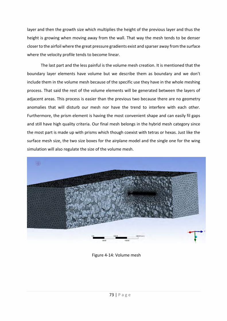
73 | P a g e
Figure 4-14: Volume mesh
layer and then the growth size which multiplies the height of the previous layer and thus the
height is growing when moving away from the wall. That way the mesh tends to be denser
closer to the airfoil where the great pressure gradients exist and sparser away from the surface
where the velocity profile tends to become linear.
The last part and the less painful is the volume mesh creation. It is mentioned that the
boundary layer elements have volume but we describe them as boundary and we don’t
include them in the volume mesh because of the specific use they have in the whole meshing
process. That said the rest of the volume elements will be generated between the layers of
adjacent areas. This process is easier than the previous two because there are no geometry
anomalies that will disturb our mesh nor have the trend to interfere with each other.
Furthermore, the prism element is having the most convenient shape and can easily fil gaps
and still have high quality criteria. Our final mesh belongs in the hybrid mesh category since
the most part is made up with prisms which though coexist with tetras or hexas. Just like the
surface mesh size, the two size boxes for the airplane model and the single one for the wing
simulation will also regulate the size of the volume mesh.

74 | P a g e
4.1.3. Solving Process
After the pre-Processing is completed and all the models are successfully meshed the
CFD cases are ready to be solved, using ANSYS-Fluent. At this section are defined the numerical
methods and the parameters of the CFD solver like the solving algorithms, the turbulence
models, the boundary conditions, the convergence criteria, the monitors of interest, the
number of iterations and anything else needed to properly solve each case. The governing
equations for the time dependent three-dimensional fluid flow and heat transfer around a
body are the continuity equation, momentum equations and energy equation. The general
approach in long range glider or uav external aerodynamics is to assume incompressible and
isothermal flow, as Ma << 0.3, which is in the velocity of 20-30m/s with common altitude
2000m and it is unlikely that the flow will reach this velocity anywhere in the domain. Thus,
the energy equation can be neglected and the momentum- and continuity equations can be
written on incompressible form, neglecting the density terms. The same solver settings are
used for all the models, so they are going to be described only once for all the cases. On the
diagram bellow are shown the steps of the solving process as they are followed for all models,
until the final results reach the desired accuracy. The steps that will be described in this
chapter can be summarized and presented in the following schematic.
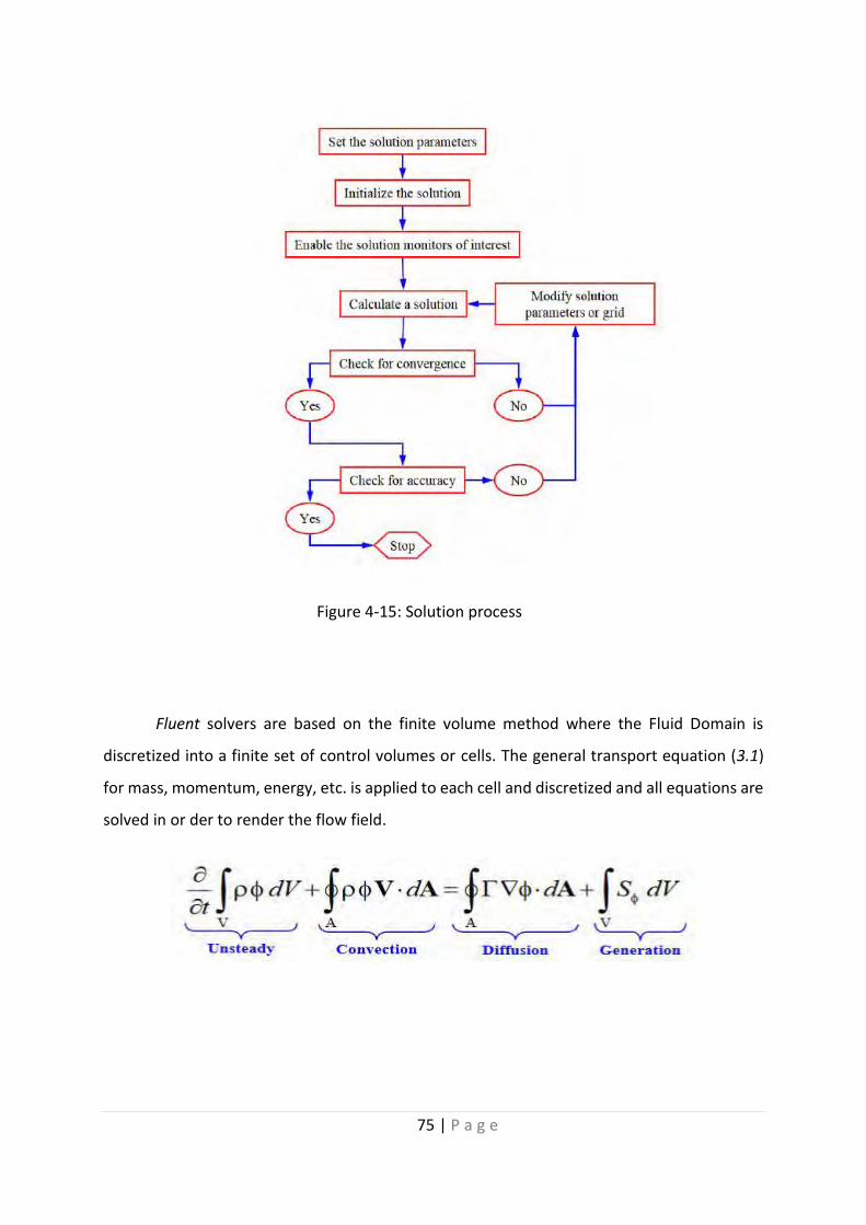
75 | P a g e
Fluent solvers are based on the finite volume method where the Fluid Domain is
discretized into a finite set of control volumes or cells. The general transport equation (3.1)
for mass, momentum, energy, etc. is applied to each cell and discretized and all equations are
solved in or der to render the flow field.
Figure 4-15: Solution process

76 | P a g e
Each transport equation is discretized into algebraic form. For a given cell, P:
Discretized equations require information at both cell centers and faces. Field data
(material properties, velocities, etc.) are stored at cell centers. Face values are interpolated in
terms of local and adjacent cell values while the discretization accuracy depends on the
“stencil” size. The discretized scalar transport equation contains the unknown scalar variable
at the cell center as well as the unknown values in surrounding neighbor cells. This equation
will, in general, be nonlinear with respect to these variables. The discretized equation (3.3)
can be expressed simply as:
where the subscript nb refers to neighbor cells, and αp and αnb are the linearized
coefficients for φ and φnb. The above equation is written for every control volume in the
domain resulting in equation sets which are solved iteratively. Coefficients αp and αnb are
typically functions of solution variables (nonlinear and coupled), they are written to use values
of solution variables from the previous iteration and they are updated with each outer
iteration.
The Pressure-Based solver is selected by default on the Solver Type field and is used
for all models. In this case, the coefficients αp and αnb are scalar values. This type of solver
employs an algorithm which belongs to a general class of methods called the projection
method. In the projection method, wherein the constraint of mass conservation (continuity)
of the velocity field is achieved by solving a pressure (or pressure correction) equation. The
pressure equation is derived from the continuity and the momentum equations in such a way
that the velocity field, corrected by the pressure, satisfies the continuity. Since the governing
equations are nonlinear and coupled to one another, the solution process involves iterations
wherein the entire set of governing equations is solved repeatedly until the solution
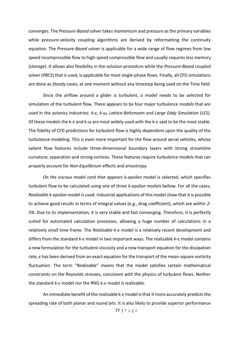
77 | P a g e
converges. The Pressure-Based solver takes momentum and pressure as the primary variables
while pressure-velocity coupling algorithms are derived by reformatting the continuity
equation. The Pressure-Based solver is applicable for a wide range of flow regimes from low
speed incompressible flow to high-speed compressible flow and usually requires less memory
(storage). It allows also flexibility in the solution procedure while the Pressure-Based coupled
solver (PBCS) that is used, is applicable for most single-phase flows. Finally, all CFD simulations
are done as Steady cases, at one moment without any timestep being used on the Time field.
Since the airflow around a glider is turbulent, a model needs to be selected for
simulation of the turbulent flow. There appears to be four major turbulence models that are
used in the avionics industries: k-ε, k-ω, Lattice-Boltzmann and Large Eddy Simulation (LES).
Of these models the k-ε and k-ω are most widely used with the k-ε said to be the most stable.
The fidelity of CFD predictions for turbulent flow is highly dependent upon the quality of the
turbulence modeling. This is even more important for the flow around aerial vehicles, whose
salient flow features include three-dimensional boundary layers with strong streamline
curvature, separation and strong vortices. These features require turbulence models that can
properly account for Non-Equilibrium effects and anisotropy.
On the viscous model card that appears k-epsilon model is selected, which specifies
turbulent flow to be calculated using one of three k-epsilon models bellow. For all the cases,
Realizable k-epsilon model is used. Industrial applications of this model show that it is possible
to achieve good results in terms of integral values (e.g., drag coefficient), which are within 2-
5%. Due to its implementation, it is very stable and fast converging. Therefore, it is perfectly
suited for automated calculation processes, allowing a huge number of calculations in a
relatively small time frame. The Realizable k-ε model is a relatively recent development and
differs from the standard k-ε model in two important ways. The realizable k-ε model contains
a new formulation for the turbulent viscosity and a new transport equation for the dissipation
rate, ε has been derived from an exact equation for the transport of the mean-square vorticity
fluctuation. The term "Realizable'' means that the model satisfies certain mathematical
constraints on the Reynolds stresses, consistent with the physics of turbulent flows. Neither
the standard k-ε model nor the RNG k-ε model is realizable.
An immediate benefit of the realizable k-ε model is that it more accurately predicts the
spreading rate of both planar and round jets. It is also likely to provide superior performance

78 | P a g e
for flows involving rotation, boundary layers under strong adverse pressure gradients,
separation, and recirculation. Both the Realizable and RNG k-ε models have shown substantial
improvements over the standard k-ε model where the flow features include strong streamline
curvature, vortices, and rotation. Since the model is still relatively new, it is not clear in exactly
which instances the Realizable k-ε model consistently outperforms the RNG model. However,
initial studies have shown that the realizable model provides the best performance of all the
k-ε model versions for several validations of separated flows and flows with complex
secondary flow features. One of the weaknesses of the Standard k-ε model or other traditional
k-ε models lies with the modeled equation for the dissipation rate (ε) limitation of the
Realizable k-ε model is that it produces non-physical turbulent viscosities in situations when
the computational domain contains both rotating and stationary fluid zone. This is due to the
fact that the Realizable k-ε model includes the effects of mean rotation in the definition of the
turbulent viscosity. This extra rotation effect has been tested on single rotating reference
frame systems and showed superior behavior over the Standard k-ε model. However, due to
the nature of this modification, its application to multiple reference frame systems should be
taken with some caution.
To understand the mathematics behind the Realizable k-epsilon model, consider
combining the Boussinesq relationship (3.4) and the Eddy Viscosity (μt) definition (3.5) to
obtain the following expression (3.6) for the normal Reynolds Stress in an incompressible
strained mean flow:

79 | P a g e
Using 3.5 equation for 𝑣𝑡=𝜇𝑡𝜌, one obtains the result that the normal stress
𝑢2̅̅̅̅̅̅̅̅̅, which by definition is a positive quantity, becomes negative, that is, “non-Realizable”,
when the strain is large enough to satisfy 3.7 equation.
The modeled transport equations for k and ε in the realizable k-ε model are:
The model constants C2, σk and σε have been established to ensure that the
model performs well for certain canonical flows. The model constants are:
The next field to be filled is the Near-Wall Treatment, which specifies the near-
wall treatment to be used for modeling turbulence. Non-Equilibrium Wall Functions is used

80 | P a g e
for all the CFD cases. The key elements in the Non-Equilibrium Wall Functions are the Launder
and Spalding’s log-law for mean velocity is sensitized to pressure-gradient effects and the two-
layer-based concept which is adopted to compute the budget of turbulence kinetic energy (𝐺𝑘̅̅̅,̅̅̅
) in the wall-neighboring cells. The log-law for mean velocity sensitized to the pressure
gradients is:
The non-equilibrium wall function employs the two-layer concept in computing the
budget of turbulence kinetic energy at the wall-adjacent cells, which is needed to solve the 𝑘
equation at the wall-neighboring cells. The wall-neighboring cells are assumed to consist of a
viscous sublayer and a fully turbulent layer. The following profile assumptions for turbulence
quantities are made:
Using these profiles, the cell-averaged production of 𝑘, 𝐺𝑘̅̅̅, and the cell-averaged
dissipation rate 𝜀̅̅̅ , can be computed from the volume average of and of the wall-adjacent
cells. For quadrilateral and hexahedral cells for which the volume average can be
approximated with a depth-average:

81 | P a g e
The next step in the simulation process is to define the boundary conditions around
the domain. Altering the boundary condition alters the whole domain solution and choosing
the proper once is an issue of vital importance for the integrity and the rightness of the results.
Besides the kind of the surface that we need to define and give some values to the speed and
the pressure on them we also need to define the turbulence intensity I in the inlet and in the
pressure outlet.
𝐼 =𝑢′
𝑈′
Where u’ is the root-mean-square of the turbulent velocity fluctuations and U is the
mean velocity. If the turbulent energy k is known u’ can be computed as:
𝑢′ = √1
3(𝑢′
𝑥2 + 𝑢′𝑦
2 + 𝑢′𝑧2) = √
2
3𝑘
Turbulence intensity varies based on the kind of problem. Consulted by the fluent
physics manuals the free stream intensity is around 1% while for cases like turbofans turbos
and propellers peaks at around 5%. Since in this simulation the propeller and its rotation will
not be included we have no reason to increase the intensity beyond 2% both on inlet and on
outlet.
The boundary conditions that the user directly applies to the problem are of two types.
The so called Dirichlet boundary condition which is a first-type and it defines the value of a
function in a specific along the chosen boundary of the
domain. This boundary condition is met in the inlet where
the velocity is specified and at the outlet where the pressure
is defined to match the altitude pressure of the flight. The
second one is the Neumann or second type boundary condition
and it is used to describe the rate of change or in more
Figure 4-16: Boundary conditions used

82 | P a g e
Figure 4-17 Curved Control Volume Inlet
mathematical terms the derivative or the gradient of the function in a boundary. This
condition is applied to all the symmetrical planes where the derivative is set to zero.
In the inlet boundary condition tab, the user can choose either to give the specified
value and the normal of the plane that the velocity vector is parallel to or to either give the
components of the velocity on each direction respectively. In the 2D simulation stage in Ansys
a commonly used technique is to create a circular inlet curve and that way the user can save
time by creating only once the mesh and then change the velocity compounds in order to
achieve the desired angle of attack in the airfoil as shown below.
But in our case since each model case will run in a different geometry and the mesh
has to be generated from the beginning the control volume has a uniform shape and to define
the inlet velocity we just need to define the amplitude of it and the normal vector to the inlet
plane will define the direction of the velocity. As mentioned above the inlet boundary

83 | P a g e
Figure 4-18: Inlet boundary condition tab
clearance has to be large enough so that the flow field in front of the object has space to
evolve and thus the stagnation points will calculate the pressure with greater precision.

84 | P a g e
The pressure outlet boundary defines the absolute static pressure that initially is
applied in all the cells of the computational grid before the iterative solution process begins.
In our case taking into consideration that the flight can occur at altitudes around 2000 meters
the density of the air at that height is equal to 1 and the atmospheric pressure is around 79.000
Pa. Both here and in the inlet section the turbulent intensity was set to 1 due to the low
Reynolds number and due to the fact that in the most area of the UAV the flow remains
undisturbed and not great mix phenomena occur.
During the pre-procession chapter, we referred that using only the half of the model
for the simulation will save us computational time and memory storage space. This symmetry
plane is defined by using the symmetry boundary condition which mathematically can be
described as
𝜕𝛷
𝜕𝑥= 0 @ 𝐵𝑢
Where the term Φ corresponds to each variable that is calculated in the boundary
(pressure, velocity, density, temperature, etc), and Bu is the boundaries where the symmetry
condition is applied.
And the final boundary condition for our external aerodynamics case is the one that
can be separated into two different conditions. This boundary condition kind is called wall and
there are a lot of different problems where it can be applied. It can either describe a stationary
wall there the no slip condition is applied or even a moving wall where the velocity of the fluid
right above the wall is equal to the translating speed of the wall. If someone has data about
the slip of the fluid, then he can also define a specific shear on that wall. In our case and
generally in airfoil study the condition is described as shown below:
�⃗� ∙ �⃗� = 0

85 | P a g e
Figure 4-19:Wall boundary condition
Where u is the velocity above the airfoil and �⃗� is the normal vector to the surface. The
component on a direction perpendicular to the surface has to be zero also known as no
penetration condition and implies that the fluid particles cannot penetrate our geometry
otherwise our geometry will be considered as a porous medium and the second one is the no
slip condition where the fluid layer right above the geometry does not slip on it.
Scheme provides a drop-down list of the available pressure-velocity coupling schemes
while as previously mentioned, the Pressure-Based solver allows to solve flow problems in
either a Segregated or Coupled manner. The Coupled algorithm is selected because it obtains
a robust and efficient single phase implementation for steady-state flows, with superior
performance compared to the segregated solution schemes. The Pressure-Based Segregated
algorithm solves the momentum equation and pressure correction equations separately, but
this semi-implicit solution method results in slow convergence. The Coupled algorithm on the
other hand, solves the momentum and pressure-based continuity equations together.
However, the memory requirement increases by 1.5 - 2 times that of the segregated algorithm
since the discrete system of all momentum and pressure-based continuity equations must be
stored in the memory when solving for the velocity and pressure fields (rather than just a

86 | P a g e
single equation, as is the case with the segregated algorithm). The full implicit coupling is
achieved through an implicit discretization of pressure gradient terms in the momentum
equations, and an implicit discretization of the face mass flux, including the Rhie-Chow
pressure dissipation terms.
In the momentum equations, the pressure gradient for component k is of the form:
Where 𝑎𝑢𝑘𝑝 is the coefficient derived from the Gauss divergence theorem and
coefficients of the pressure interpolation schemes. Finally, for any 𝑖th cell, the discretized form
of the momentum equation for component 𝑢𝑘 is defined as:
As a result, the overall system of equations (3.18) and (3.19), after being
transformed to the δ-form, is presented as:
where the influence of a cell 𝑖 on a cell 𝑗 has the form:
Spatial Discretization contains settings that control the spatial discretization of the
convection terms in the solution equations. Gradient contains a drop-down list of the options
for setting the method of computing the gradient. Gradients are needed not only for
constructing values of a scalar at the cell faces, but also for computing secondary diffusion
terms and velocity derivatives. The gradient 𝛻𝜑 of a given variable 𝜑 is used to discretize the
convection and diffusion terms in the flow conservation equations. The Least Squares Cell-
Based gradient method t is selected and used for all the CFD models. In this method, the
solution is assumed to vary linearly. In Cell Centroid Evaluation, the change in cell values
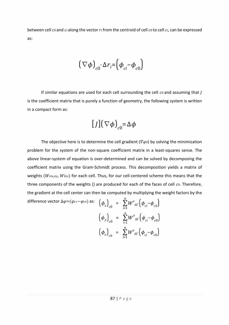
87 | P a g e
between cell 𝑐0 and 𝑐𝑖 along the vector 𝑟𝑖 from the centroid of cell 𝑐0 to cell 𝑐𝑖, can be expressed
as:
If similar equations are used for each cell surrounding the cell 𝑐0 and assuming that 𝐽
is the coefficient matrix that is purely a function of geometry, the following system is written
in a compact form as:
The objective here is to determine the cell gradient (𝛻𝜑0) by solving the minimization
problem for the system of the non-square coefficient matrix in a least-squares sense. The
above linear-system of equation is over-determined and can be solved by decomposing the
coefficient matrix using the Gram-Schmidt process. This decomposition yields a matrix of
weights (𝑊𝑖0𝑥,0𝑦, 𝑊𝑖0𝑧) for each cell. Thus, for our cell-centered scheme this means that the
three components of the weights () are produced for each of the faces of cell 𝑐0. Therefore,
the gradient at the cell center can then be computed by multiplying the weight factors by the
difference vector Δ𝜑=(𝜑𝑐1−𝜑𝑐0) as:

88 | P a g e
Figure 4-20: Meshing refinement process
After the initialization of every case that we run the spatial discretization technique
that we did use was the first order upwind for the pressure and momentum and after 100
iterations we chose the second order one. The above technique was used during our
experience with the FSAE aerodynamics team and it was observed to give faster convergence.
4.1.4. Mesh Dependency
While using finite differences or finite volume or finite element methods someone can
tell that the denser the computational grid the more accurate our solution and our simulation
prediction will be. At some point though our solution will converge to a certain value and
further increasing the number of our elements will have no practical meaning to our solution
we need to find a point where our solution is no longer mesh depended. This will help us keep
the calculation time low and will save us a lot of time. Our mesh independency plan started
by using the default mesh as a starting point with no size boxes placed in the geometry
domain. The next step was to place some size boxes around our wing and decrease both locally
and globally the average volume element size as well as the surface element size on the wing.
During this process the number of the boundary layer elements was constant and the mesh
densing strategy is shown in the table and diagrams below. For all the simulations we used
the PSU airfoil placed in 6 degrees angle of attack and at 10m/s flying speed.
We can see that the mesh refinement procedure took into consideration both the
volume element size and the face element size. Both of them have impact on the solution
since greater number of face elements means that we have a more precise expression of the
pressure field above the wing the when the surface integration happens we have more
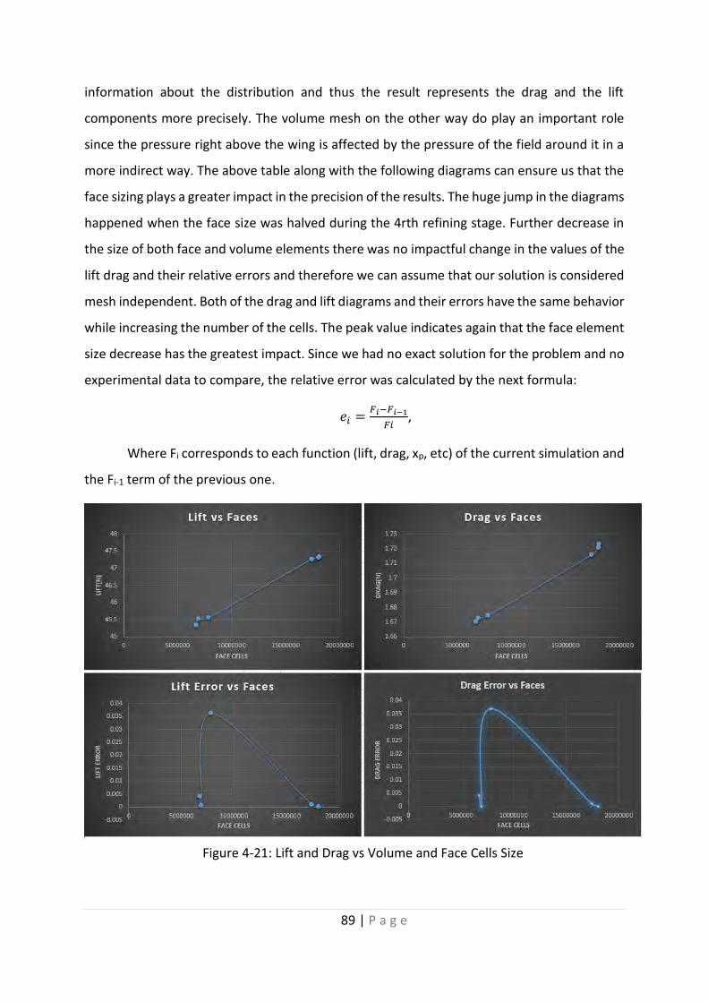
89 | P a g e
Figure 4-21: Lift and Drag vs Volume and Face Cells Size
information about the distribution and thus the result represents the drag and the lift
components more precisely. The volume mesh on the other way do play an important role
since the pressure right above the wing is affected by the pressure of the field around it in a
more indirect way. The above table along with the following diagrams can ensure us that the
face sizing plays a greater impact in the precision of the results. The huge jump in the diagrams
happened when the face size was halved during the 4rth refining stage. Further decrease in
the size of both face and volume elements there was no impactful change in the values of the
lift drag and their relative errors and therefore we can assume that our solution is considered
mesh independent. Both of the drag and lift diagrams and their errors have the same behavior
while increasing the number of the cells. The peak value indicates again that the face element
size decrease has the greatest impact. Since we had no exact solution for the problem and no
experimental data to compare, the relative error was calculated by the next formula:
𝑒𝑖 =𝐹𝑖−𝐹𝑖−1
𝐹𝑖,
Where Fi corresponds to each function (lift, drag, xp, etc) of the current simulation and
the Fi-1 term of the previous one.

90 | P a g e
Figure 4-22: Lift and Drag vs Volume and Volume Cells Size
When plotting the relative error of a function having the exact solution using a
stable scheme we can observe that the function follows a constant increase or decrease path
towards zero (for the relative error) even if the error fluctuates around the path. This is a
healthy way of reducing the relative error without convergence issues. In our case though the
relative error is calculated based on the current value of the function and therefore we can
observe this huge peak in the diagrams. On the other hand, the lift and drag diagrams have
no such issue since the greater the mesh resolution the closer we get to the mesh independent
solution and in a very linear way.
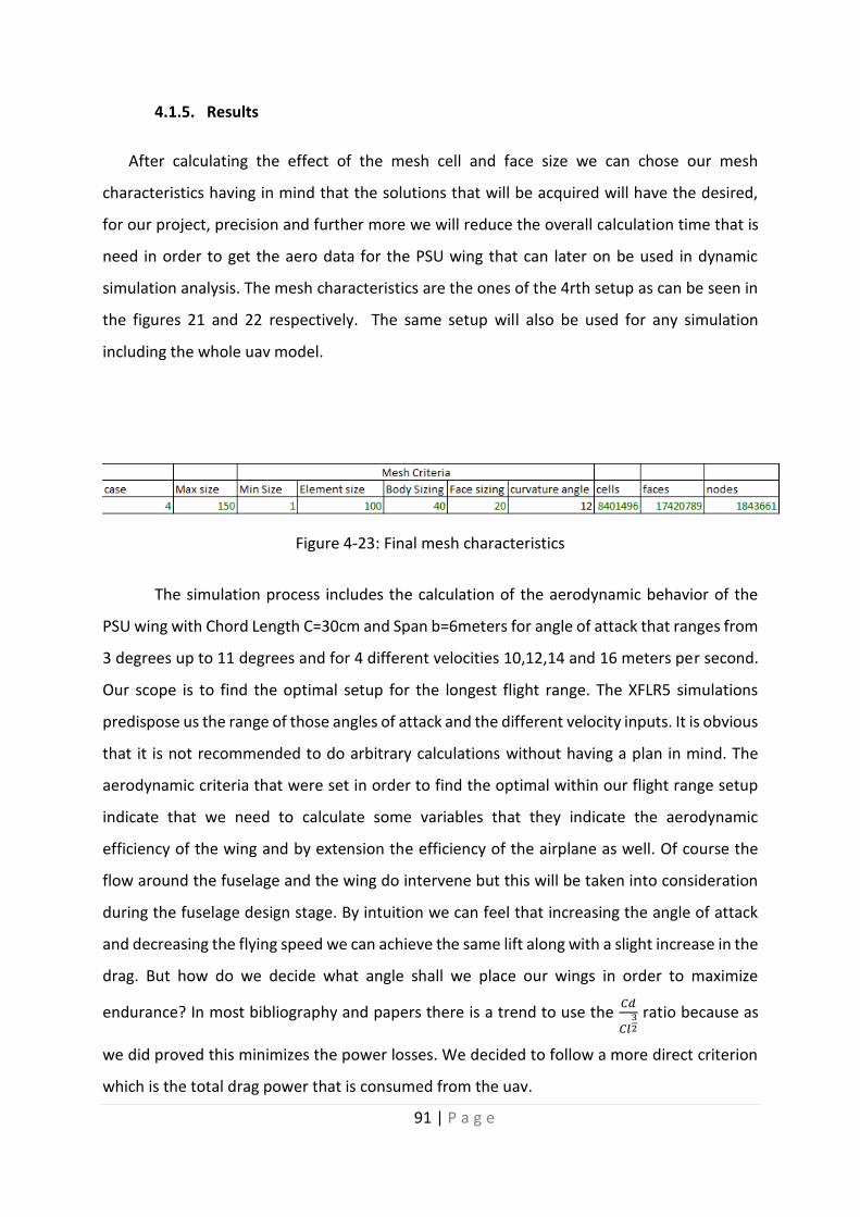
91 | P a g e
Figure 4-23: Final mesh characteristics
4.1.5. Results
After calculating the effect of the mesh cell and face size we can chose our mesh
characteristics having in mind that the solutions that will be acquired will have the desired,
for our project, precision and further more we will reduce the overall calculation time that is
need in order to get the aero data for the PSU wing that can later on be used in dynamic
simulation analysis. The mesh characteristics are the ones of the 4rth setup as can be seen in
the figures 21 and 22 respectively. The same setup will also be used for any simulation
including the whole uav model.
The simulation process includes the calculation of the aerodynamic behavior of the
PSU wing with Chord Length C=30cm and Span b=6meters for angle of attack that ranges from
3 degrees up to 11 degrees and for 4 different velocities 10,12,14 and 16 meters per second.
Our scope is to find the optimal setup for the longest flight range. The XFLR5 simulations
predispose us the range of those angles of attack and the different velocity inputs. It is obvious
that it is not recommended to do arbitrary calculations without having a plan in mind. The
aerodynamic criteria that were set in order to find the optimal within our flight range setup
indicate that we need to calculate some variables that they indicate the aerodynamic
efficiency of the wing and by extension the efficiency of the airplane as well. Of course the
flow around the fuselage and the wing do intervene but this will be taken into consideration
during the fuselage design stage. By intuition we can feel that increasing the angle of attack
and decreasing the flying speed we can achieve the same lift along with a slight increase in the
drag. But how do we decide what angle shall we place our wings in order to maximize
endurance? In most bibliography and papers there is a trend to use the 𝐶𝑑
𝐶𝑙32
ratio because as
we did proved this minimizes the power losses. We decided to follow a more direct criterion
which is the total drag power that is consumed from the uav.
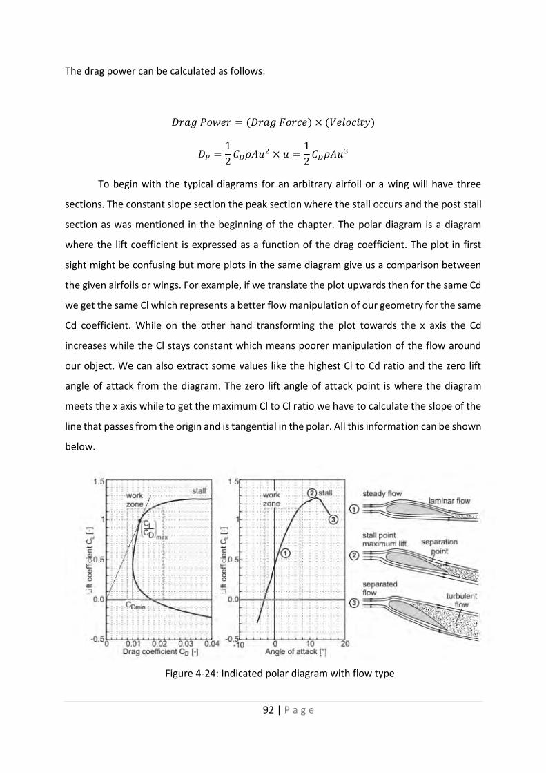
92 | P a g e
Figure 4-24: Indicated polar diagram with flow type
The drag power can be calculated as follows:
𝐷𝑟𝑎𝑔 𝑃𝑜𝑤𝑒𝑟 = (𝐷𝑟𝑎𝑔 𝐹𝑜𝑟𝑐𝑒) × (𝑉𝑒𝑙𝑜𝑐𝑖𝑡𝑦)
𝐷𝑃 =1
2𝐶𝐷𝜌𝐴𝑢2 × 𝑢 =
1
2𝐶𝐷𝜌𝐴𝑢3
To begin with the typical diagrams for an arbitrary airfoil or a wing will have three
sections. The constant slope section the peak section where the stall occurs and the post stall
section as was mentioned in the beginning of the chapter. The polar diagram is a diagram
where the lift coefficient is expressed as a function of the drag coefficient. The plot in first
sight might be confusing but more plots in the same diagram give us a comparison between
the given airfoils or wings. For example, if we translate the plot upwards then for the same Cd
we get the same Cl which represents a better flow manipulation of our geometry for the same
Cd coefficient. While on the other hand transforming the plot towards the x axis the Cd
increases while the Cl stays constant which means poorer manipulation of the flow around
our object. We can also extract some values like the highest Cl to Cd ratio and the zero lift
angle of attack from the diagram. The zero lift angle of attack point is where the diagram
meets the x axis while to get the maximum Cl to Cl ratio we have to calculate the slope of the
line that passes from the origin and is tangential in the polar. All this information can be shown
below.

93 | P a g e
Figure 4-25: PSU Lift vs AoA for different speed values
Figure 4-26: PSU Lift vs AoA for different speed values
All the graphs that follow can describe the aerodynamic behavior of our wing
within the velocity and angle range that was given during the simulation process. One can also
calculate the aerodynamic coefficients or the lift and drag forces of the wing by interpolating
the values that are already calculated and get the desired values.

94 | P a g e
Figure 4-27: PSU Drag vs Angle of attack Figure 4-28 :PSU Cd vs Angle of attack
When the speed and by extension the Reynolds number increases we can expect an
increase in the lift coefficient value since the circulation will increase and thus the flow
transition point from laminar to turbulent will delay to appear on the airfoil and thus
increasing the total lift that can be generated. This can also be achieved by increasing the
thickness of the airfoil. Greater thickness will increase the u+ (the velocity on the upper wing
section) and thus again the transition point will be aft the previous one. One more important
aspect of the PSU choice is the linear section of the lift and as shown below drag amplitude in
the area of 3-5 degrees. This will not alter neither the total amount of power that is consumed
for small angle of attack fluctuations nor its lift that is produced decreasing the oscillations
while midair.
Efficiency is the most desirable aspect of our geometry especially for a MALE
(medium altitude long endurance) uav. The two variables that describe the efficiency of an
object that is moving inside a fluid are the:
𝐶𝑙
𝐶𝑑
And the term:

95 | P a g e
Figure 4-30 PSU minimum power efficiency factor Figure 4-29 PSU Cl to Cd ratio
Figure 4-31: Drag Power vs AoA
𝐶𝑑
𝐶𝑙
32
The second term is not something that can be intuitively understood but was extracted
by minimum power consumption criterion in chapter 3.2
Finally, the most direct endurance criterion of an object is the power consumption
itself. It was calculated based on the drag force and the velocity of the flight and lets no space
for misunderstanding and misleading on what is the optimal setup of the geometrical variables
that we need to be defined. It can also be used as an optimization criterion.

96 | P a g e
Figure 4-32: PSU drag power consumption
It is obvious that increasing the angle of attack of a wing then the drag increases since
the vector of the total force is pointing more backwards and thus the component of the drag
is greater, what we are interested in this graph is the behavior of the power consumption at
a given speed for a range of angles like previously. The more constant the power consumption
then the more accurate predictions we can make for the average consumption of the wing
since it does not have a constant angle of attack but it fluctuated throughout the flight. But
the selection of the desired uflight which is the speed that the glider will fly and the angle of
attack of the main wing can be done by looking the next graph.
The horizontal axis of the graph indicates the power consumption while on the y axis
we can see the total amount of lift that can be produced while we spent the equivalent x axis
power. The blue horizontal line indicates the estimated weight that was calculated during the
weight estimation process. Thus all the points that are above the line are points where the lift
produced can lift the weight of the plane and thus the plane flies or accelerates while the
points below the line represent the points where the lift is less than the weight and the uav
starts to decelerate and decent. We want to pick the point that is borderline above the weight
estimation line and has the fewest consumption of drag power. The point of minimum power
that can produce adequate lift is the 2nd point of the orange curve. Which is at 3.5 degrees

97 | P a g e
Figure 4-33 : Elliptical vs Rectangular Cl distribution
angle of attack and 12 m/s flying speed. Thus, this will be the target flying speed and the angle
that the wing placement angle.
4.2. 3D Wing Design
In the introduction in this chapter there was a short representation of the most wing
geometrical parameters and values that define its geometry. Now the whole simulation
process was done only by altering the velocity and the angle of attack of the given PSU wing
and no alter in its shape took place. The factors that can alter its geometry are the taper ratio,
the twist of the wing, the dihedral angle, the swept ratio and the placement or not of winglets
in the ends of the wings. Of course, the changes that we will make have no arbitrary character
but the purpose of them is to ensure that the flow around the wing is the closest to the
optimal.
4.2.1. Elliptic Distribution
As can be seen the figure 33 shows the distribution of section lift coefficients, Cl, along
the span of some arbitrary wing planform. The figure shows the frontal view of a cantilevered
wing (the left wing is shown, looking toward the leading-edge). The plane of symmetry (left)
is where the wing root would be located and the right side is the left wingtip. The figure 34
shows two kinds of distribution of Cl. The first can be considered an ideal span wise
distribution, which would be achieved if the laws of physics didn’t require the lift to gradually
go to zero at the wingtip. This distribution would result in each span wise station contributing
uniformly to the total lift coefficient. As a consequence, it would require the least amount of
AoA at any given airspeed to maintain altitude. And the less the AoA, the less is the generation
of lift-induced drag.

98 | P a g e
Figure 4-34: Elliptical vs Uniform Lift Distribution
4.2.2. Wing Parameters
A way to achieve the elliptical wing distribution is to create a wing with an elliptical
span wise chord distribution. Another way of achieving this distribution is by altering the
shape even the profile of the airfoil when reaching the wingtip. In order for the wing to
generate the same amount of lift we can place the profile of the airfoil closer to the fuselage
in a higher angle of attack. That way we change the lift distribution and we reduce some lift
from the tip of the wing, and we add it closer to the fuselage. One drawback of this is that the
stall will start to occur closer to the fuselage since the airfoil there will be placed in higher
angle of attack. But it is the only way as long as the wing must retain its chord for two rows of
solar panels to be fitted.

99 | P a g e
The analysis began with the initial orthogonal shaped wing. The wing has been
designed in the XFLR5, putting the parameters such as (0.3m) chord, (6m) span and zero
sweep, dihedral and wing twist, as seen below.
After designing the wing, the first step is to select the polar type of the analysis. By
selecting Fixed Lift analysis, the code calculates the speed and the other aerodynamic
coefficients for a fixed value of lift, making it easy for the comparison after a change in
geometry through the optimal solution. The Vortice Lattice Method (VLM2) has been used as
it is the most accurate method and the only one that considers viscous forces. The mass of the
airplane was inputted 10 kilograms, as it initially calculated.
Figure 4-35: Wing Design

100 | P a g e
Figure 4-387: Analysis Method
Figure 4-36: Polar type
Figure 4-37: Analysis method
Figure 4-39: Mass selection of the airplane

101 | P a g e
The span wise lift distribution of the orthogonal shaped wing, as seen below, was far
from an elliptical distribution, so we tried reducing lift from the tips of the wing by putting a
symmetric airfoil as the last section of the wing, in zero angle of attack.
Figure 4-40: Orthogonal Shaped Wing & Induced Drag Distribution
Figure 4-41: Orthogonal Wing, Lift Distribution

102 | P a g e
The outcome of the next run is better and the induced drag is reduced due to
reducing of wing tip vortices. The procedure that was followed afterwards was a sequence of
changing the twist of the wing in the points that the lift needed reduction, until the target
curve is achieved.
Figure 4-42: Orthogonal Wing With Horizontal Winglets, Lift Distribution
Figure 4-43: Orthogonal Wing With Horizontal Winglets

103 | P a g e
Figure 4-45: Orthogonal Wing With Horizontal Winglets & Twist
Figure 4-44: Orthogonal Wing With Horizontal Winglets & Twist, Lift Distribution

104 | P a g e
Figure 4-46: Orthogonal Wing With Horizontal Winglets & Twist, version II
Figure 4-47: Orthogonal Wing With Horizontal Winglets & Twist, version II, Lift Distribution

105 | P a g e
Figure 4-48: Orthogonal Wing With Horizontal Winglets & Twist, version III
Figure 4-49: Orthogonal Wing With Horizontal Winglets & Twist, version III, Lift Distribution

106 | P a g e
Chapter5: Fuselage
Fuselage is the central portion of the body of an airplane, designed to accommodate
the crew, passengers, and cargo. It varies greatly in design and size according to the function
of the aircraft. In a jet fighter the fuselage consists of a cockpit large enough only for the
controls and pilot, but in a jet airliner it includes a much larger cockpit as well as a cabin that
has separate decks for passengers and cargo. The fuselage also serves to position control and
stabilization surfaces in specific relationships to lifting surfaces, which is required for aircraft
stability and manoeuvrability.
Once having decided the airfoil profile as well as the parameters of the wing we
obtained the lift generating device. So one of the major fuselage purpose use is to provide
adequate rigidity so that it can withstand the static and dynamic loads during the flight and in
our case to house all the electrical components needed in order for the UAV to flight in a
controllable manner. Before analysing the geometry and the type of the fuselage we have to
take into consideration some aspects and features that our plane requires. The major ones
are:
Fineness ratio to avoid large pressure gradients and flow separation
Ease of removing and replacing electrical components
Rigidity
Streamlined design for low drag generation and moment balancing
Proper wing placement so that COG is aft of the COP
Do not obstruct the folding of the propeller blades
The aircraft fineness ratios are defined as length divided by diameter, which including nose
fineness ratios and tail cone fineness ratios. In all of the following nose cone shape equations
L is the overall length of the nose cone and R is the radius of the base of the nose cone. Y is
the radius at any point x, as x varies from 0, at the tip of the nose cone, to L. The equations
define the 2-dimensional profile of the nose shape. The full body of revolution of the nose
cone is formed by rotating the profile around the centerline (C/L). Note that the equations
describe the 'perfect' shape practical nose cones are often blunted or truncated for
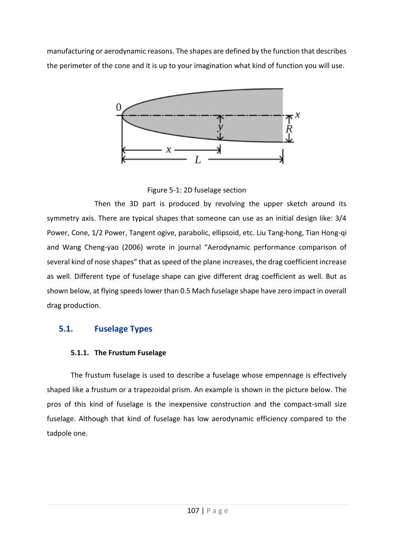
107 | P a g e
manufacturing or aerodynamic reasons. The shapes are defined by the function that describes
the perimeter of the cone and it is up to your imagination what kind of function you will use.
Figure 5-1: 2D fuselage section
Then the 3D part is produced by revolving the upper sketch around its
symmetry axis. There are typical shapes that someone can use as an initial design like: 3/4
Power, Cone, 1/2 Power, Tangent ogive, parabolic, ellipsoid, etc. Liu Tang-hong, Tian Hong-qi
and Wang Cheng-yao (2006) wrote in journal “Aerodynamic performance comparison of
several kind of nose shapes” that as speed of the plane increases, the drag coefficient increase
as well. Different type of fuselage shape can give different drag coefficient as well. But as
shown below, at flying speeds lower than 0.5 Mach fuselage shape have zero impact in overall
drag production.
5.1. Fuselage Types
5.1.1. The Frustum Fuselage
The frustum fuselage is used to describe a fuselage whose empennage is effectively
shaped like a frustum or a trapezoidal prism. An example is shown in the picture below. The
pros of this kind of fuselage is the inexpensive construction and the compact-small size
fuselage. Although that kind of fuselage has low aerodynamic efficiency compared to the
tadpole one.

108 | P a g e
Figure 5-2: Frustum fuselage type
5.1.2. The Pressure Tube Fuselage
The look of that fuselage is pretty familiar since the most of the passenger airplanes
are designed like this. It consists of three parts the two capped sections in the front and the
rear of the airplane and a cigar like cylinder in the middle. The circular middle section is ideal
for carrying pressure loads and therefore is used in high altitude avionics. One drawback is
that the huge diameter of the fuselage as well as the sloped aft (so that it does not touch the
ground during take-off) is that they create turbulent wake decreasing the effectiveness of the
rudder. Ways to avoid this phenomenon is to add a dorsal or vertical fin between the fuselage
and the rudder but since this type is not appropriate for our purpose no further analysis will
take place.
Figure 5-3: Pressure Tube Fuselage Vs Angle of Attack

109 | P a g e
5.1.3. Tadpole Fuselage
As the name of this fuselage implies the shape of it is similar to a tadpole. It consists of
an ellipsoidal cabin in the front a lofted lever to connect the fuselage with the empennage,
the wings and the empennage itself. Tadpole fuselages generate far less drag than the frustum
kind for two primary reasons: (1) their forward portion is shaped to sustain laminar boundary
layer and (2) their empennage shape results in as much as 30-40% less wetted area, where
wetted area is the portion of the control surfaces that are affected from the turbulent wake.
Figure 5-4: Frustum vs Tadpole Fuselage Ref. Althaus D. Motorless Flight Research
In low Reynolds numbers like in our case a big fraction of the total drag is created by
the shear stresses in the fuselage circumference and the rest is created from the pressure
difference between the rear and the front face of the fuselage. Another aspect of tadpole
fuselage design is the downward tilt of the fuselage as shown in the next figure. This is a
response to the upwash caused in the airflow ahead of the wing. A straight fuselage will be at
a higher angle of incidence and this will increase its drag. To reduce this, the forward portion

110 | P a g e
of the fuselage is tilted downward to align it with the oncoming airflow, reducing its drag.
Some further efficiency increase can be achieved by tilt the tail-boom down or reshape it to
better match the flow behind the wing as well.
This phenomenon occurs at relatively high velocities which are translated to lower
pressure on the upper area of the wings. In our case we have to take into consideration and
other aspects before we rework our model like the fact that the upper area of the wings is
quite distant from the nosecone of the fuselage and at low Reynolds flights the upwash that
is created has not that much of an effect in the overall drag. Furthermore, as it was said in
previous chapter in low Reynolds flows a decent amount of drag is caused by the fluid friction.
Thus, we can decrease the amplitude of drag by simply making a more compact with smaller
surface fuselage.
One more influential aspect of the design, is the wash that the propeller can generate
by creating a vortex like rotational wake that will affect the wing that lies right behind it. It is
a drawback that all the propeller propulsed aerial vehicles have to deal with, and the most
common way to counter its effect is to place the propeller in the rear of the fuselage. This
though comes with great disadvantages like the moment that the propeller force produces,
does not constitute to self-aligning torque making the whole aircraft more unstable since it
not only tends to rotate the construction around the pitch axis and it also leaves dirty air for
the ailerons and the ruder making the passive and active control more difficult and the control
Figure 5-5: Upwash effect in the fuselage
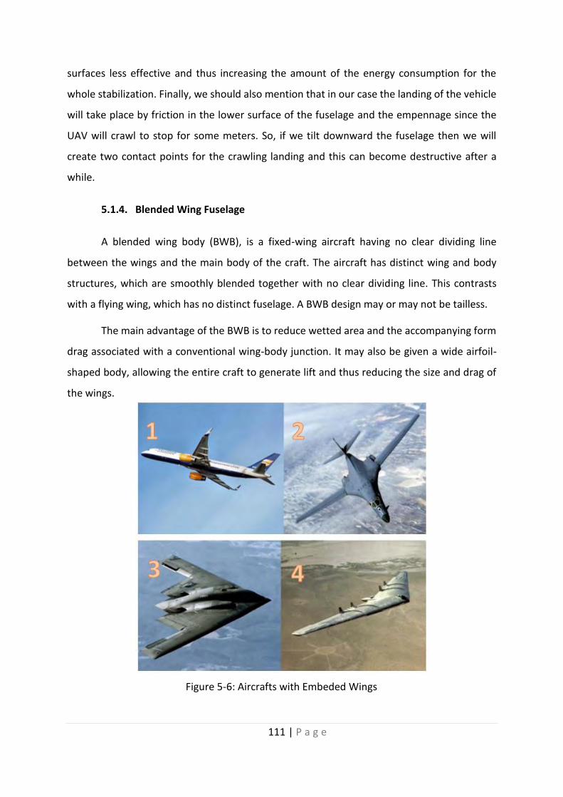
111 | P a g e
Figure 5-6: Aircrafts with Embeded Wings
surfaces less effective and thus increasing the amount of the energy consumption for the
whole stabilization. Finally, we should also mention that in our case the landing of the vehicle
will take place by friction in the lower surface of the fuselage and the empennage since the
UAV will crawl to stop for some meters. So, if we tilt downward the fuselage then we will
create two contact points for the crawling landing and this can become destructive after a
while.
5.1.4. Blended Wing Fuselage
A blended wing body (BWB), is a fixed-wing aircraft having no clear dividing line
between the wings and the main body of the craft. The aircraft has distinct wing and body
structures, which are smoothly blended together with no clear dividing line. This contrasts
with a flying wing, which has no distinct fuselage. A BWB design may or may not be tailless.
The main advantage of the BWB is to reduce wetted area and the accompanying form
drag associated with a conventional wing-body junction. It may also be given a wide airfoil-
shaped body, allowing the entire craft to generate lift and thus reducing the size and drag of
the wings.

112 | P a g e
5.2. Fuselage Design
After the possible concepts were taken into consideration, the geometry of the
fuselage has to be designed. The first thing is to design the electronic components assembly
in that way so the Center of Gravity will be as far forward as possible and in the aircraft
symmetry plane.
Figure 5-7: Electronics Assembly
Figure 5-8: Electronics Assembly Zoomed In
Motor
Motor Controller Energy
Management
System
Li-ion Battery Cells
Flight Controller
Reveiver
Transmitter

113 | P a g e
So the Li-ion batteries divided in two pairs, each fitted in a wing and the other
electronic components have put along the roll axis so the aircraft is balanced. The first concept
to be applied is the tadpole shaped fuselage that is efficient and with minimal design since the
already designed wing can be attached straight to the fuselage.
The fuselage designed around the electronic components with as less frontal
area as possible for minimum aerodynamic drag. Another limitation was that the (600mm)
diameter propeller has to be folded in when the motor shuts down. The design process can
be shown to the figures below.
Figure 5-9: Electronics Assembly with Sketched Fuselage Around Them
Figure 5-10: Tadpole/Cylindrical Fuselage

114 | P a g e
Figure 5-12: Tadpole/Cylindrical Fuselage with Wings Attached
Figure 5-11: Tadpole/Cylindrical Fuselage
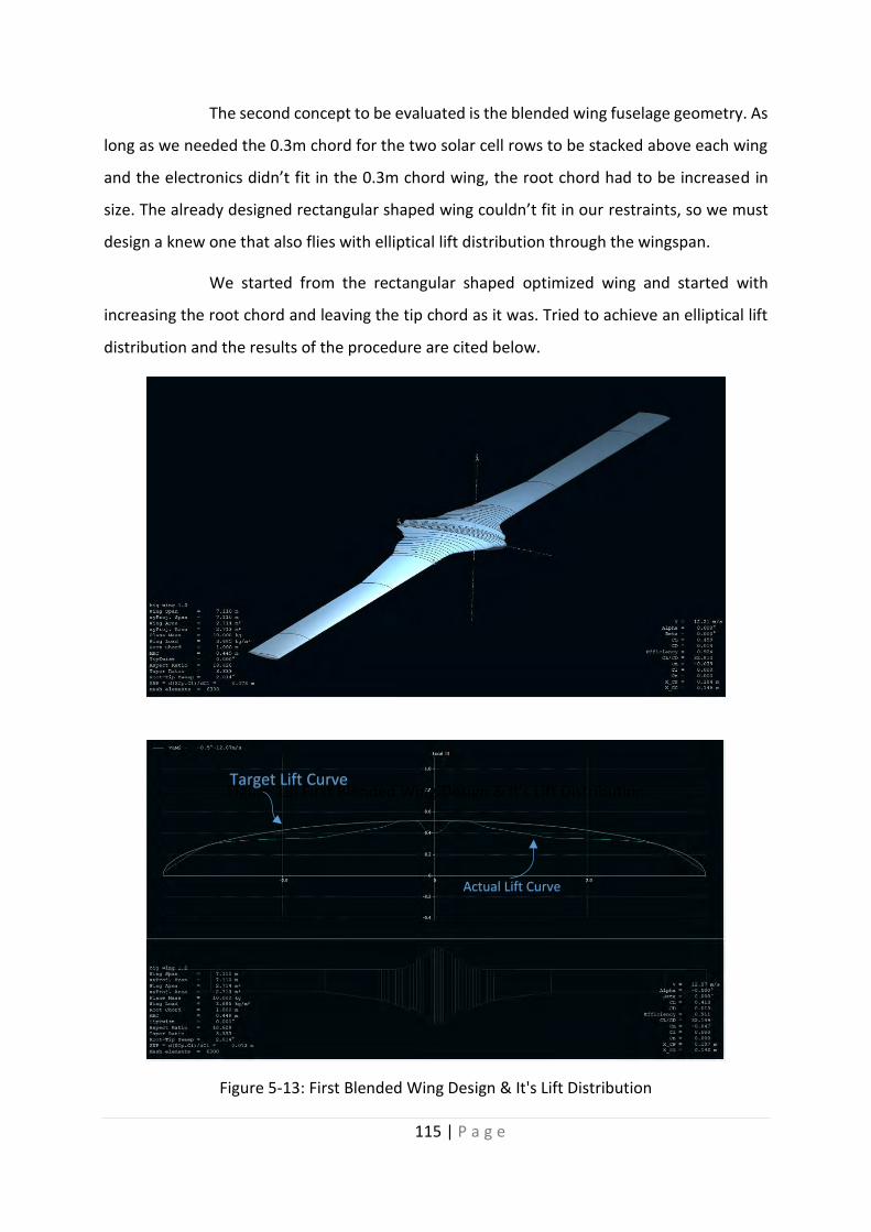
115 | P a g e
Figure 5-13: First Blended Wing Design & It's Lift Distribution
The second concept to be evaluated is the blended wing fuselage geometry. As
long as we needed the 0.3m chord for the two solar cell rows to be stacked above each wing
and the electronics didn’t fit in the 0.3m chord wing, the root chord had to be increased in
size. The already designed rectangular shaped wing couldn’t fit in our restraints, so we must
design a knew one that also flies with elliptical lift distribution through the wingspan.
We started from the rectangular shaped optimized wing and started with
increasing the root chord and leaving the tip chord as it was. Tried to achieve an elliptical lift
distribution and the results of the procedure are cited below.
Figure 13: First Blended Wing Design & It's Lift Distribution
Target Lift Curve
Actual Lift Curve

116 | P a g e
Figure 5-15: 3rd Design Lift Distribution
Figure 5-14: 2nd Design Lift Distribution

117 | P a g e
Figure 5-16: 4th Design Lift Distribution

118 | P a g e
Figure 5-17: Final Design Lift Distribution
The simulation in the XFLR5 was executed for fixed “10kg” lift, and the results were
the speed that the aircraft must fly, as also its aerodynamic coefficients. As soon as the elliptic
lift distribution was achieved the next step was the comparison of the two optimized Wing-
Fuselage concepts so that can be selected the one with the smaller drag force.
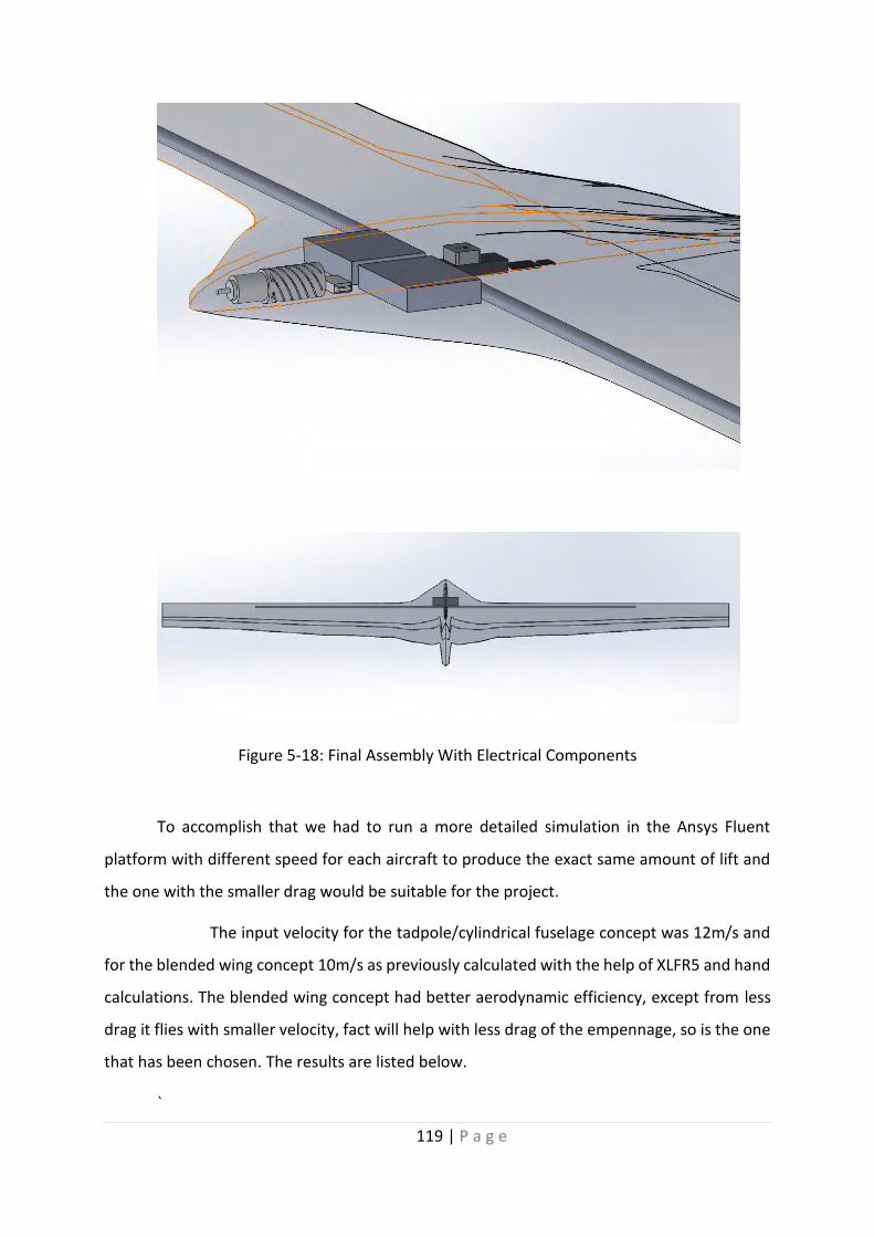
119 | P a g e
Figure 5-18: Final Assembly With Electrical Components
To accomplish that we had to run a more detailed simulation in the Ansys Fluent
platform with different speed for each aircraft to produce the exact same amount of lift and
the one with the smaller drag would be suitable for the project.
The input velocity for the tadpole/cylindrical fuselage concept was 12m/s and
for the blended wing concept 10m/s as previously calculated with the help of XLFR5 and hand
calculations. The blended wing concept had better aerodynamic efficiency, except from less
drag it flies with smaller velocity, fact will help with less drag of the empennage, so is the one
that has been chosen. The results are listed below.
`

120 | P a g e
Figure 5-19: Blended Wing
Tadpole/ Cylindrical Concept Blended Wing Concept
Pressure Viscous Total Pressure Viscous Total
DRAG[N] 1.49 2.08 73.5 1.53 1.77 3.30
LIFT[N] 101.32 0.058 101.38 98.94 0.055 98.99
POWER[W] 42.84 33
Figure 5-20: Tadpole/Cylindrical Concept

121 | P a g e
Figure 5-21: Blended Wing Fuselage Concept

122 | P a g e
Chapter6: Tail Design and Stability
6.1. Stable Flight
Until this point we have chosen a proper airfoil for our high efficiency flight, we altered
the geometry of the wing to match the elliptical lift distribution achieving minimum induced
drag generation and we designed a fuselage that its purpose is to hold all the electrical
components and actuators that the UAV need in order to operate. The next major step is to
make the flight of our vehicle as smooth as possible. The importance of the stability analysis
is vital to every vehicle and system that operates under transient conditions and is called to
reject possible disturbances while trying to reach the set point that the user stations. For
example, our aerial vehicle needs to stay at a certain level during its flight and damp any
oscillations along the 3 axis because that way will be flying in the desired operational point
which is designed to have maximum efficiency. Our stability analysis consists of three parts.
Load case: Every possible combinations of angles in each axis causes the flow over
the UAV to create moments and forces around the center of mass. Acquiring these
data will give us the aero map of the construction. To achieve this, we need to run
simulations for each angle change on each direction and the problem is that during the
simulation we cannot simplify our model by using a symmetry plane. Furthermore, the
forces that act on an object that moves inside a fluid are proportional to the square of
the velocity. This means that the steady state simulation will not provide us with
adequate data. Therefore, a transient simulation has to be set in order to get the right
moments around the 3 axis.
Dynamics of a UAV: After the data have been acquired there is further need for a
dynamic simulation to take place. The environment of Simulink allows for a dynamic
simulation by simulating the system with a 6 DOF block. The simulation considers that
the forces acting on the body do not create moment coupling in a random axis but only
around the center of mass. That way we can consider the center of mass as a fixed
point for every axis.

123 | P a g e
Figure 6-1: Two different scenarios at high AoA and small AoA
Empennage: The empennage term is used to describe the tail of the glider which can
be broken in two parts the vertical one and the horizontal one. The length that they
will be placed at, the area of the control surfaces and the type of the airfoil that will be
used defines the response of the system at any changes. To make things simpler the
whole concept is to create a greater moment around the center of mass with the
smallest possible deflection of the empennage. The moment is defined as a Force that
acts on a distance from the rotation axis. The force itself of the empennage is a
function of its area, the rotational speed and the lever that the force is placed at
relative to the center of rotation. Therefore, a compensation has to be made between
the area of the control surfaces and the location of them behind the wing.
PID tuning: The PID is a great field of automation study and provides the users the
ability to control the response characteristics of a system. For example, we can change
the behavior of the system by altering the values of the PID constants. We can make a
system faster but with greater error of the set point or reduce the overshooting with
compensating to the rise time which is the time that the system needs to reach the set
point. The PID controllers here are not different physical objects and should not be
confused with the PWM controllers of the motor. They are embedded inside the flying
controller each one for the set of moving control areas. The tuning that needs to be
done is to define the parameters for each set and the tuning method will not provide
any information for the moving areas but it will only optimize their function on the
overall stability.
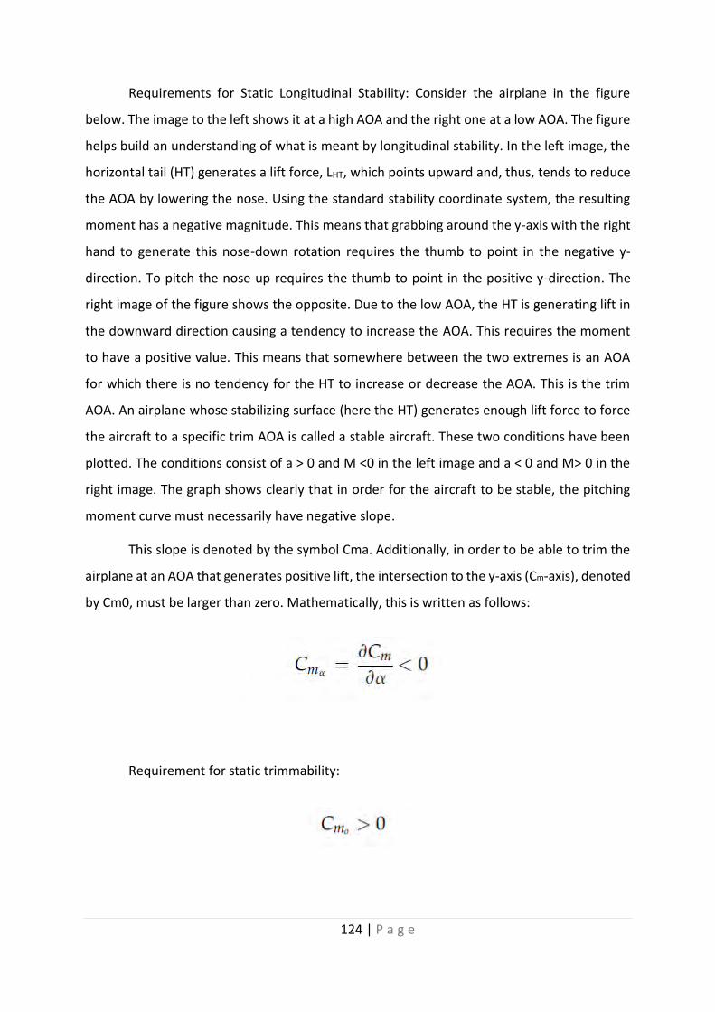
124 | P a g e
Requirements for Static Longitudinal Stability: Consider the airplane in the figure
below. The image to the left shows it at a high AOA and the right one at a low AOA. The figure
helps build an understanding of what is meant by longitudinal stability. In the left image, the
horizontal tail (HT) generates a lift force, LHT, which points upward and, thus, tends to reduce
the AOA by lowering the nose. Using the standard stability coordinate system, the resulting
moment has a negative magnitude. This means that grabbing around the y-axis with the right
hand to generate this nose-down rotation requires the thumb to point in the negative y-
direction. To pitch the nose up requires the thumb to point in the positive y-direction. The
right image of the figure shows the opposite. Due to the low AOA, the HT is generating lift in
the downward direction causing a tendency to increase the AOA. This requires the moment
to have a positive value. This means that somewhere between the two extremes is an AOA
for which there is no tendency for the HT to increase or decrease the AOA. This is the trim
AOA. An airplane whose stabilizing surface (here the HT) generates enough lift force to force
the aircraft to a specific trim AOA is called a stable aircraft. These two conditions have been
plotted. The conditions consist of a > 0 and M <0 in the left image and a < 0 and M> 0 in the
right image. The graph shows clearly that in order for the aircraft to be stable, the pitching
moment curve must necessarily have negative slope.
This slope is denoted by the symbol Cma. Additionally, in order to be able to trim the
airplane at an AOA that generates positive lift, the intersection to the y-axis (Cm-axis), denoted
by Cm0, must be larger than zero. Mathematically, this is written as follows:
Requirement for static trimmability:

125 | P a g e
Figure 6-2: Plot of the two scenarios Cm vs AoA
If these conditions are satisfied, then there exists an AOA > 0 for which the Cm is equal
to zero. The importance of AOA > 0 is that the vehicle can generate lift in the opposite direction
of the weight and simultaneously be statically stable.
The next thing that we have to check is the corresponding stability around the yaw axis
(directional stability). Directional stability is the capability of the vehicle to weather vane.
Imagine standing behind an actual weather vane with the wind directly in your face. If the
vane is rotated so its nose points, say, right (and the tail points left) intuition tells us its tail
will generate lift that points to the right, in the positive y-direction (see depiction in the
upcoming figure). This, in turn, generates a moment whose tendency is to rotate the nose left
and align it (and the tail) with the wind. Since the moment corrects the alignment, it is said to
be restoring. If the above weather vane is yawed nose right, then, using the stability
coordinate system (SCS), the angle b< 0o. This means that if looking along the centerline of the
vane, the wind would strike the left cheek. The restoring moment is negative because per the
right hand rule, the resulting rotation is analogous to grabbing around the z-axis with the right
hand to rotate it with the right thumb pointing upward e in the negative z-direction. The
opposite holds true if the weather vane is rotated nose left e a positive moment (thumb

126 | P a g e
pointing down) is then required to bring the nose right to the initial position. As we can see
from the figure it shows how this establishes requirements for static directional stability. It
turns out that in order for this correcting tendency to be realized, the slope of the yawing
moment curve must have a positive slope. Mathematically this is written as follows:
Requirement for static directional stability:
Next consider lateral stability (see the figure below). It differs from both longitudinal
and directional stability in that it requires sideslip (or yaw), and not roll itself, to be corrected
(ignoring the application of devices like ailerons). This is the aforementioned dihedral effect.
The geometric features of airplanes are such that when flying asymmetrically a restoring
rolling as well as directional moments are created. It is the responsibility of the designer to
decide how to manipulate the geometry to make these moments restoring or convergent (and
not diverging). Dihedral effect has many sources as will become evident shortly. Consider the
airplane in the upper left part of the figure, whose nose points to the right of the wind
direction (which is normal to the plane). For now, consider only the contribution of the wing
to the rolling moment. It can be seen from the top view in the lower left corner that the left
wing leads the right one. This causes asymmetric loading on the wing that generates more lift
on the left wing than the right one. The difference creates a rolling moment that tends to lift
the leftwing and bring it back to level. The rolling moment is positive because, according to
the right-hand rule, the resulting moment vector points forward (the thumb would point
forward) along the positive x-axis. The opposite holds if the nose is yawed to the left so the
rightwing leads the left one; a negative moment is created. By plotting a line between those
two conditions it can be seen that the rolling moment must have a negative slope in order to
be stable. Mathematically:
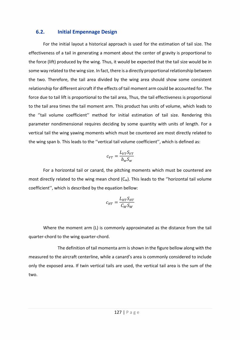
127 | P a g e
6.2. Initial Empennage Design
For the initial layout a historical approach is used for the estimation of tail size. The
effectiveness of a tail in generating a moment about the center of gravity is proportional to
the force (lift) produced by the wing. Thus, it would be expected that the tail size would be in
some way related to the wing size. In fact, there is a directly proportional relationship between
the two. Therefore, the tail area divided by the wing area should show some consistent
relationship for different aircraft if the effects of tail moment arm could be accounted for. The
force due to tail lift is proportional to the tail area, Thus, the tail effectiveness is proportional
to the tail area times the tail moment arm. This product has units of volume, which leads to
the ‘’tail volume coefficient’’ method for initial estimation of tail size. Rendering this
parameter nondimensional requires deciding by some quantity with units of length. For a
vertical tail the wing yawing moments which must be countered are most directly related to
the wing span b. This leads to the ‘’vertical tail volume coefficient’’, which is defined as:
𝑐𝑉𝑇 =𝐿𝑉𝑇𝑆𝑉𝑇
𝑏𝑤𝑆𝑤
For a horizontal tail or canard, the pitching moments which must be countered are
most directly related to the wing mean chord (Cw). This leads to the ‘’horizontal tail volume
coefficient’’, which is described by the equation bellow:
𝑐𝐻𝑇 =𝐿𝐻𝑇𝑆𝐻𝑇
𝐶𝑊𝑆𝑊
Where the moment arm (L) is commonly approximated as the distance from the tail
quarter-chord to the wing quarter-chord.
The definition of tail momenta arm is shown in the figure bellow along with the
measured to the aircraft centerline, while a canard’s area is commonly considered to include
only the exposed area. If twin vertical tails are used, the vertical tail area is the sum of the
two.
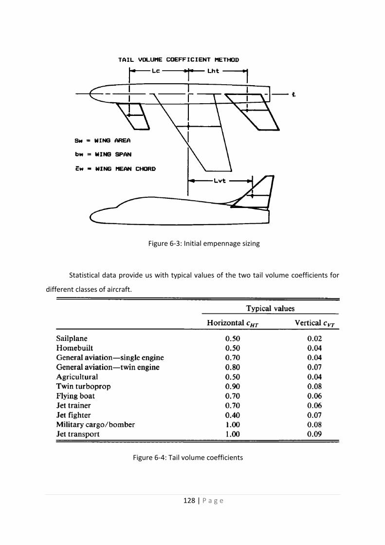
128 | P a g e
Figure 6-4: Tail volume coefficients
Statistical data provide us with typical values of the two tail volume coefficients for
different classes of aircraft.
Figure 6-3: Initial empennage sizing

129 | P a g e
𝑆𝑉𝑇 = 𝑐𝑉𝑇𝑏𝑤𝑆𝑤/𝐿𝑉𝑇
𝑆𝐻𝑇 = 𝐶𝐻𝑇𝐶𝑊𝑆𝑊/𝐿𝐻𝑇
To calculate the tail size, the moment arm must be estimated. This can be
approximated at this stage of design by a percent of the fuselage length as previously
estimated. For an aircraft with a front-mounted propeller, Raymer proposes, the tail arm is
about 60% of the fuselage length. For an aircraft with the engines on the wings, the tail arm is
about 50-55% of the fuselage length. For aft-mounted engines the tail arm is about 45-50% of
the fuselage length. A sailplane has a tail movement arm of about 65% of the fuselage length.
Our UAV type can be related to the sailplane and since we need steady with not great response
characteristics plane the 65% is the case for us. The problem with our case is that the above
methodology needs an estimation for the fuselage which is based on same methods that rely
on the thrust to weight ratio that the sailplane is called to reach. With those numbers and
since our UAV has a great moment of inertia around the y axis the vertical tail had to be
enormous for the responses of the above methodology. The initial design is presented in the
following figures.

130 | P a g e
Table 6-1: Initial empennage sizing, input parameters
Table 6-2: Initial empennage sizing, output parameters
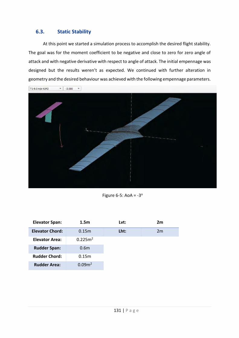
131 | P a g e
6.3. Static Stability
At this point we started a simulation process to accomplish the desired flight stability.
The goal was for the moment coefficient to be negative and close to zero for zero angle of
attack and with negative derivative with respect to angle of attack. The initial empennage was
designed but the results weren’t as expected. We continued with further alteration in
geometry and the desired behaviour was achieved with the following empennage parameters.
Elevator Span: 1.5m Lvt: 2m
Elevator Chord: 0.15m Lht: 2m
Elevator Area: 0.225m2
Rudder Span: 0.6m
Rudder Chord: 0.15m
Rudder Area: 0.09m2
Figure 6-5: AoA = -3o
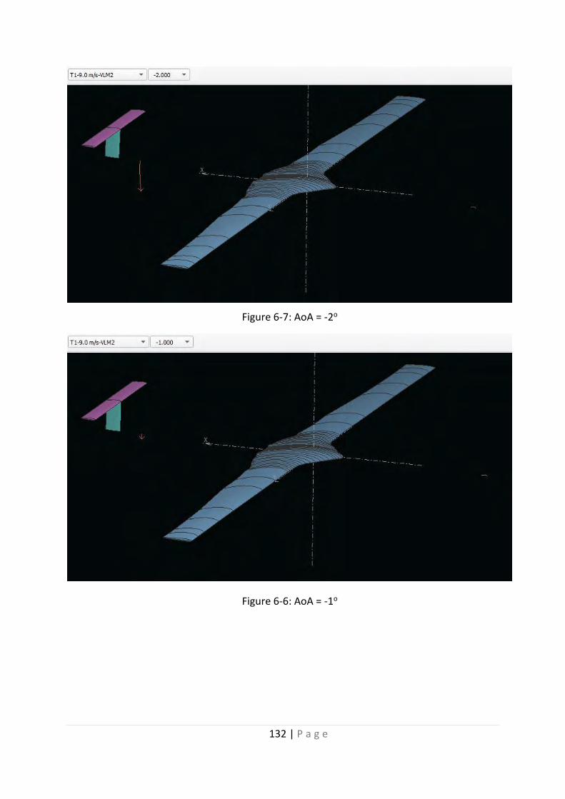
132 | P a g e
Figure 6-7: AoA = -2o
Figure 6-6: AoA = -1o

133 | P a g e
Figure 6-9: AoA=0o
Figure 6-8: AoA = 1o

134 | P a g e
Figure 6-11: AoA = 2 o
Figure 6-10: Cm vs AoA in final empennage design

135 | P a g e
6.4. Dynamic Stability
After the aircraft proven statically stable, it must be tested for dynamic stability as well.
The dynamic stability analysis took place in XFLR5 and the procedure is described in the
upcoming paragraphs. Α well-designed aircraft has 4 natural longitudinal modes and 4 natural
lateral modes.
Longitudinal Lateral
2 symmetric phugoid modes
2 symmetric short period modes
1 spiral mode
1 roll damping mode
2 Dutch roll modes
Phugoid modes: The longer period mode, called the "phugoid mode" is the one
in which there is a large-amplitude variation of air-speed, pitch angle, and altitude, but almost
no angle-of-attack variation. The phugoid oscillation is a slow interchange of kinetic energy
(velocity) and potential energy (height) about some equilibrium energy level as the aircraft
attempts to re-establish the equilibrium level-flight condition from which it had been
disturbed. The motion is so slow that the effects of inertia forces and damping forces are very
low. Although the damping is very weak, the period is so long that the pilot usually corrects
for this motion without being aware that the oscillation even exists. Typically, the period is
20–60 seconds. This oscillation can generally be controlled by the pilot.
Figure 6-12: Phugoid modes
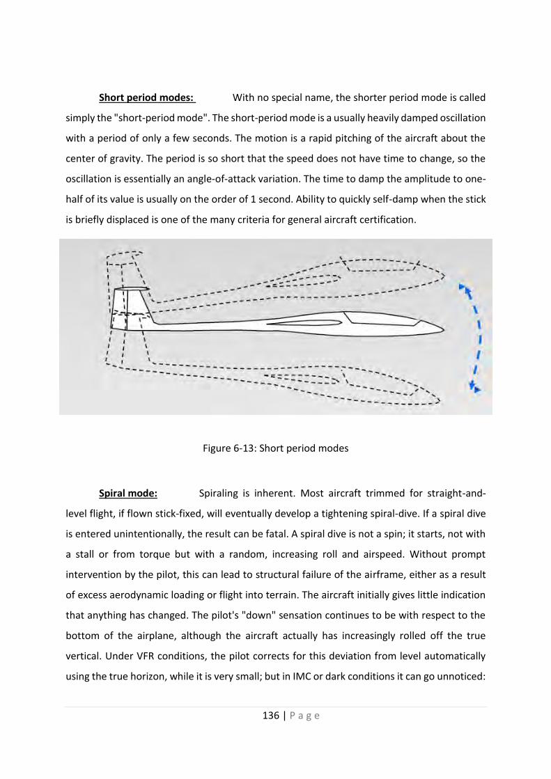
136 | P a g e
Short period modes: With no special name, the shorter period mode is called
simply the "short-period mode". The short-period mode is a usually heavily damped oscillation
with a period of only a few seconds. The motion is a rapid pitching of the aircraft about the
center of gravity. The period is so short that the speed does not have time to change, so the
oscillation is essentially an angle-of-attack variation. The time to damp the amplitude to one-
half of its value is usually on the order of 1 second. Ability to quickly self-damp when the stick
is briefly displaced is one of the many criteria for general aircraft certification.
Figure 6-13: Short period modes
Spiral mode: Spiraling is inherent. Most aircraft trimmed for straight-and-
level flight, if flown stick-fixed, will eventually develop a tightening spiral-dive. If a spiral dive
is entered unintentionally, the result can be fatal. A spiral dive is not a spin; it starts, not with
a stall or from torque but with a random, increasing roll and airspeed. Without prompt
intervention by the pilot, this can lead to structural failure of the airframe, either as a result
of excess aerodynamic loading or flight into terrain. The aircraft initially gives little indication
that anything has changed. The pilot's "down" sensation continues to be with respect to the
bottom of the airplane, although the aircraft actually has increasingly rolled off the true
vertical. Under VFR conditions, the pilot corrects for this deviation from level automatically
using the true horizon, while it is very small; but in IMC or dark conditions it can go unnoticed:

137 | P a g e
the roll will increase and the lift, no longer vertical, is insufficient to support the airplane. The
nose drops and speed increases: the spiral dive has begun.
Figure 6-14: Spiral mode
Roll damping mode: Roll subsidence mode is simply the damping of rolling
motion. There is no direct aerodynamic moment created tending to directly restore wings-
level, i.e. there is no returning "spring force/moment" proportional to roll angle. However,
there is a damping moment (proportional to roll rate) created by the slewing-about of long
wings. This prevents large roll rates from building up when roll-control inputs are made or it
damps the roll rate (not the angle) to zero when there are no roll-control inputs. Roll mode
can be improved by dihedral effects coming from design characteristics, such as high wings,
dihedral angles or sweep angles.

138 | P a g e
Figure 6-15: Roll damping mode
Dutch roll modes: The second lateral motion is an oscillatory combined roll
and yaw motion called Dutch roll, perhaps because of its similarity to an ice-skating motion of
the same name made by Dutch skaters; the origin of the name is unclear. The Dutch roll may
be described as a yaw and roll to the right, followed by a recovery towards the equilibrium
condition, then an overshooting of this condition and a yaw and roll to the left, then back past
the equilibrium attitude, and so on. The period is usually on the order of 3–15 seconds, but it
can vary from a few seconds for light aircraft to a minute or more for airliners. Damping is
increased by large directional stability and small dihedral and decreased by small directional
stability and large dihedral. Although usually stable in a normal aircraft, the motion may be so
slightly damped that the effect is very unpleasant and undesirable. In swept-back wing
aircraft, the Dutch roll is solved by installing a yaw damper, in effect a special-purpose
automatic pilot that damps out any yawing oscillation by applying rudder corrections. Some
swept-wing aircraft have an unstable Dutch roll. If the Dutch roll is very lightly damped or
unstable, the yaw damper becomes a safety requirement, rather than a pilot and passenger
convenience. Dual yaw dampers are required and a failed yaw damper is cause for limiting
flight to low altitudes, and possibly lower Mach numbers, where the Dutch roll stability is
improved.

139 | P a g e
Figure 6-16: Ditch roll modes
These natural modes describe the aircraft’s response on its natural frequencies,
without any pilot’s or flight controller’s interference.
The code running in XFLR5:
Searches the angle of attack such that Cm=0
Calculates the trim speed to achieve a steady flight
Evaluates the stability derivatives
Extracts the eigenvalues
In the results we can see the time response in relevance to the variables that
describe the aircraft’s state at any instant. The four longitudinal variables are:
u is the variation of speed along the x-axis
w is the variation of speed along the z-axis
q is the pitch rate, i.e. the rotation vector around the y-axis
θ is the pitch angle, i.e. the angle between the stability x-axis and the horizontal flight
line, the angle is positive for a nose up.
The four lateral variables are:
v is the variation of speed along the w-axis
p is the roll rate, i.e. the rotation vector around the x-axis
r is the yaw rate, i.e. the rotation vector around the z-axis

140 | P a g e
φ is the bank angle, i.e. the angle between the stability y-axis and the horizontal flight
line, the angle is positive for a right wing down.
Figure 6-17: Longitudinal mode I, Short period mode
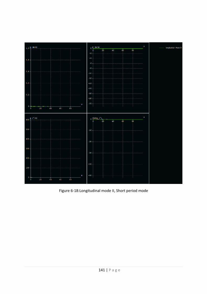
141 | P a g e
Figure 6-18:Longitudinal mode II, Short period mode
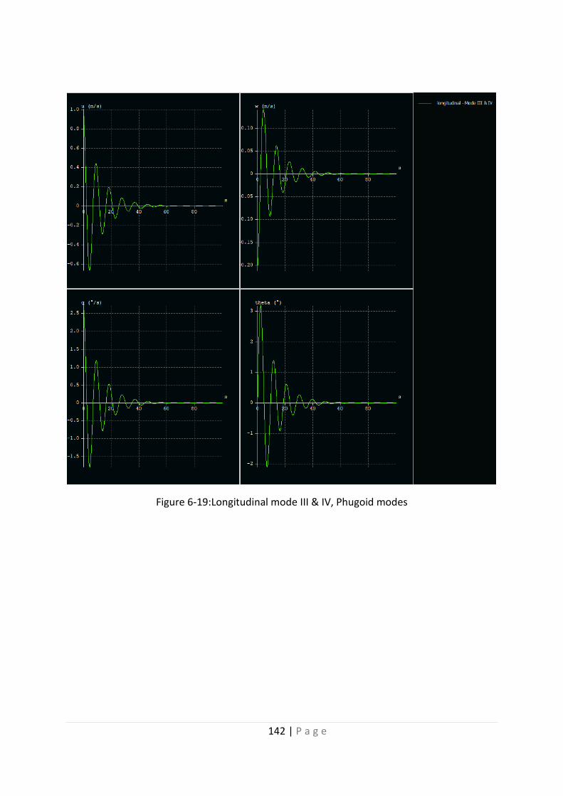
142 | P a g e
Figure 6-19:Longitudinal mode III & IV, Phugoid modes

143 | P a g e
Figure 6-20:Lateral mode I, Roll damping mode

144 | P a g e
Figure 6-21:Lateral mode II & III, Dutch roll modes

145 | P a g e
Figure 6-22:Lateral mode IV, Spiral mode

146 | P a g e
Figure 6-23: Root locus diagram for eigenvalues
+
All modes except spiral, lead to dynamic stability, which is the goal of this analysis.
Spiral mode is a common result to come to divergence and it’s up to pilot or flight controller
to bring the aircraft in stability. This is a primary dynamic stability analysis that indicates a
generally stable aircraft without the intervention of the controller.
Longitudinal Lateral
Spiral
Dutch Roll
Dutch Roll
Roll Short Period
Short Period
Phugoid
Phugoid

i | P a g e
Chapter7:
7.1. Conclusion
After all the simulations that took place both in aerodynamics and stability area we
can tell that we achieved our goal. The embedded wings UAV can fly with a power
consumption of 35.7 watt taking into consideration the drag power of the tail. Furthermore
because of the embedded wing design some extra area that was not taken into consideration
has come up and add 12 extra solar cells in the tail and another 18 cells on the body of the
UAV. Furthermore because of the summer period that the flight will take place we have some
thermal ascending air currents that will gain us altitude without the need of motor spinning.
The Pixhawk flight controller has integrated thermal searching mode where the plane can only
glide and absorb energy without wasting any at moving the propeller. Finally there was
enough space for some extra panels both on the fuselage and the horizontal stabilizer. Thus
the amount of the panels was raised in 136 and the total energy that is fed to the system is
97.75.
Solar Panels Area
m2
Power
Watt
Drag Power Watt
136 2.125 97.75 35
As we can see from the data presented in the table above the total power balance has
a positive result in our system.
7.2. Future work
7.2.1. Experimental Setup
The experimental setup is a necessity for the validation process before
proceeding into the manufacturing of the wing. It allows for data to be acquired and compared
with the simulation once leaving no room for errors if the experiment is set properly. Due to
the time limitation we did not bring the experiment into life and left as future work.

ii | P a g e
7.2.2. Dynamic Simulation with Control Area Sizing and PID Tuning
The static stability chapter was complete in all of three axis (Yaw, Pitch and Roll) and
the UAV provides a decent passive stability as a construction. The further that someone needs
to enrich the dynamic stability by introducing the flaps, elevators, rudders, and ailerons of the
plane in order to make its response more accurate or fast. To do so a dynamic 6DOF model
has to be set in Simulink. We have to refer that the Pixhawk flight controller has embedded
onboard real life PID tuning and therefore only some initial values are need in order for the
first ascent to take place. Then the auto tuning takes over and defines the gains of each term
for the desired response characteristics. If that is not possible then some initial values can be
found based on Roskam initial sizing method for the actuation areas.
Figure 7-1: Final Model Design

iii | P a g e
Chapter8: APENDIX
Figure 8-1:Aquila9.3
Figure 8-2:E374
Figure 8-3:E387
Figure 8-4:EH2_10
Figure 8-5:EPPLER423
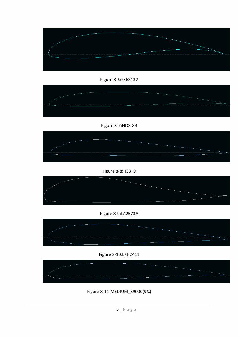
iv | P a g e
Figure 8-6:FX63137
Figure 8-7:HQ3-8B
Figure 8-8:HS3_9
Figure 8-9:LA2573A
Figure 8-10:LKH2411
Figure 8-11:MEDIUM_S9000(9%)
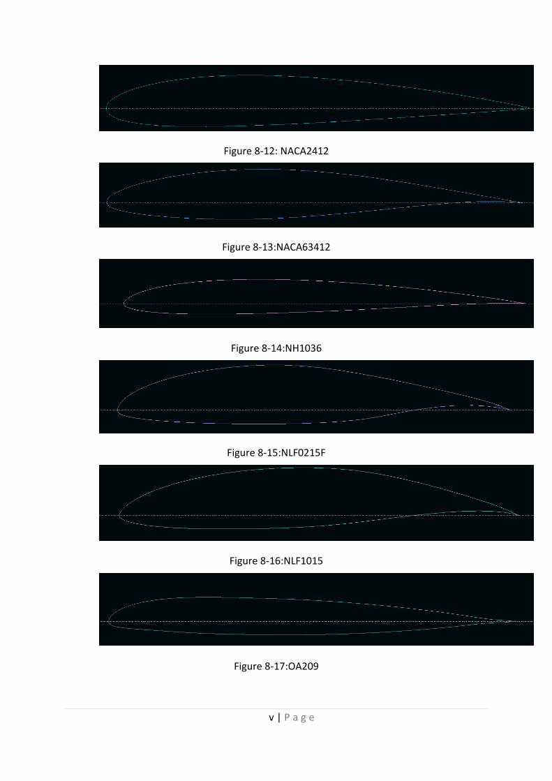
v | P a g e
Figure 8-12: NACA2412
Figure 8-13:NACA63412
Figure 8-14:NH1036
Figure 8-15:NLF0215F
Figure 8-16:NLF1015
Figure 8-17:OA209

vi | P a g e
Figure 8-18:PHOENIX
Figure 8-19:PSU94-097
Figure 8-20:S510
Figure 8-21:S905
Figure 8-22:SELIG1223

vii | P a g e
Figure 8-23:S9037
Figure 8-24:SA7038
Figure 8-25:SD7032
Figure 8-26:SG6040

viii | P a g e
Figure 8-27:SG6042
Figure 8-28:WE3.55

ix | P a g e
Table 8-1: Geometrical Parameters of the Final Wing
x | P a g e
Chapter9: Bibliography
A. Weider, H. L. (2006). SunSailor: Solar Powered UAV.
Bruscoli, S. (2011). Airfoil Optimization for a Solar Powered Aircraft.
D.Raymer. (1992). Aircraft Design. A Conceptual Approach.
Eun-Mi Kwon, K.-H. Y.-J.-Y. (2011). Design Considerations and Modeling of a Small and Low
Altitude Solar Powered UAV.
Gudmundsson, S. (2014). General Aviation Aircraft Design Applied Methods and Procedures.
http://www.airfoiltools.com. (n.d.).
J.Hartney, C. (2011). DESIGN OF A SMAL SOLAR-POWERED UNMANNED AERIAL VEHICLE.
Johansson, M. (2011). Project Solaris – Construction of Solar.
Joseph Katz, A. P. (2001). Low speed aerodynamics.
Karthik Reddy Buchireddy Sri, P. A. (2016). Design Analysis of Solar-Powered Unmanned Aerial
Vehicle.
Lan, D. J.-T. (1997). Airplane Aerodynamics and Performance.
Lee, K. (2004). DEVELOPMENT OF UNMANNED AERIAL VEHICLE (UAV).
NOTH, A. (2008). Design of Solar Powered Airplanes.
P. Panagiotou, P. K. (2016). Aerodynamic design of a MALE UAV.
Parvathy Rajendran, H. S. (2016). Modelling of solar irradiance and daylight duration for solar-
powered UAV sizing.
Pedro David Bravo-Mosquera, L. B.-B.-G.-M. (2017). Aerodynamic design analysis of a UAV for
superficial research.
Poonsong, P. (2004). DESIGN AND ANALYSIS OF A MULTI-SECTION VARIABLE CAMBER WING.
Sultan, A. (2011). Project Solaris - The Design of a Solar Powered UAV.
Tsagarakis, M. (2011). Project Solaris – Analysis of airfoil for solar powered flying wing UAV.
Vinayak Bembrekar, A. R. (2018). Design of a Wing with Bell-shaped Span-load using VLM
Method.

xi | P a g e
Weisheng Chen, L. P. (2008). Design and Performance of Low Reynolds Number Airfoils.
(http://www.airfoiltools.com, n.d.)

xii | P a g e


