ADRESSE : FASEG/UCAD, BP : 47337 Dakar-Liberté, Dakar, Sénégal
SITE INTERNET : www.larem-ucad.org
Seydi Ababacar DIENG
Adjusted Net Savings (ANS) and economic
growth in WAEMU
Document de travail n° 14
Avril 2015
LAREM – UCAD
Sénégal
ECOLE DOCTORALE SCIENCES
JURIDIQUES, POLITIQUES,
ECONOMIQUES ET DE GESTION
(ED-JPEG)
UNIVERSITE CHEIKH
ANTA DIOP DE DAKAR
LABORATOIRE DE RECHERCHES
ECONOMIQUES ET MONETAIRES
Résumé
L’objectif de cet article est de mesurer la contribution de l’ENA dans la croissance
économique des pays de l’UEMOA. Les résultats de l’estimation du modèle de données de panel à
effets communs ont révélé, contrairement à l’hypothèse retenue, que le coefficient de l’ENA par tête
est négatif et significatif au seuil de 5 %.Ainsi, d'une année à l'autre, si la croissance de l'ENA baisse
de 0,105 point, alors, ceteris paribus, la croissance du PIB augmente d'un point. Ce résultat peint
fidèlement la situation des pays de l’UEMOA, caractérisée par une tendance baissière dans presque
tous les pays de la zone. Cette baisse est la conséquence de l'épuisement des ressources forestières,
énergétiques, minières et les dommages causés par la pollution. Or cet épuisement des ressources –
exploitation des mines pour créer de la richesse – et ces dommages dus à la pollution – utilisation des
véhicules pour le transport des marchandises – contribuent grandement à l'accroissement du PIB.
Les résultats ont aussi montré le rôle positif et très significatif au seuil de 1 % de la formation
brute de capital fixe (FBCF) sur le taux de croissance économique de l’UEMOA. Ainsi, une
augmentation de 1 % de la FBCF par tête génère une croissance par tête supplémentaire de 0,527
point. Ces résultats devraient conduire les autorités communautaires, notamment la BCEAO, à créer
les conditions favorables à l’accroissement de l’ENA.
Classification JEL : O550, C130
Abstract
The objective of this paper is to measure the contribution of ANS in the economic growth of
the WAEMU countries. The results of the estimate to the common effects panel data model revealed,
contrary to the assumption that the ANS head coefficient is negative and significant at the 5%
threshold. Thus, from one year to another, if the NAS growth down 0.105 points then, ceteris paribus,
increases GDP growth by one point. This result faithfully painted the situation in WAEMU countries,
characterized by a downward trend in almost all countries in the region. This decrease is a
consequence of the depletion of forest resources, energy, mining and damage caused by pollution.
Now this resource depletion - Mining to create wealth - and the damage caused by pollution - use of
vehicles for the transport of goods – contribute greatly to GDP growth.
The results also showed positive and significant role in the 1% of gross fixed capital formation
(GFCF) on the economic growth of the WAEMU. Thus, a 1% increase in GFCF per capita growth
generates additional head 0.527 points. These results should lead the Community authorities, including
the BCEAO, to create conditions favorable to the growth of the NAS.
JEL Classification : O550, C130
1
Introduction
Several reports - including those of Brundtland (1987) and IPCC (2015) - have
particularly highlighted the degradation of soil quality, depletion of resources, pollution and
climatic disturbances1. These facts constitute credible threats to the environment and thus ultimately
on the future of the human species. These have promoted economic development approach taking greater account of environmental capital and advocating a rational use of resources and respect for
nature. It is in this perspective that the concept of adjusted net savings (ANS) was developed and proposed by the World Bank.
ANS or genuine savings integrates different forms of capital - physical, human and naturally to assess the level of sustainability or sustainable development of countries
2. Pearce and Atkinson (1993)
were the first to offer an empirical illustration of the ANS.
According to the World Bank (1999) ANS is equal to net national saving - corresponding strictly
to physically capital increased human capital accumulation and reduced depletion of the stock of natural resources and damage caused by pollution - carbon dioxide and particulate pollutants. Human
capital is considered here only to current expenditure on education. The theories underlying the ANS are optimal growth and weak sustainability property. Sustainability can be defined as maintaining or increasing social welfare, apprehended by the value of
all components of the ANS. The weak sustainability property stipulates the substitutability of different
components of the ANS. Thus, a decrease in the natural resource base can be offset by investment in
human or physical capital gains from the exploitation of some of these3: it is the rule of Hartwick
(1974) or Hicks rule-Solow-Hartwick or weak sustainability rule. Hamilton and Clemens (1999) and
Dasgupta Mäler (2000) and Asheim and Weitzman (2001) are the main authors that contributed to
the ENA theory.
The richness of this concept - especially compared to traditional national savings - and
issues relating to the future of humanity and its ecosystem justify the interest that we should
give him, especially for the developing countries (DCs ) and in particular the countries of the
West Africa Economic and Monetary Union (WAEMU). Indeed, WAEMU countries are
mainly based on long-term renewable resources to develop. But sustainable development
seems to necessarily pass through the promotion of ANS, including through its environmental
component. This leads us naturally to study the impact of ANS on economic growth in
WAEMU countries.
The relevance and legitimacy of this question resident, first, in the fact that the various
theories of growth have shown the important role of the three components of the ANS in
economic growth4. Then, two recent empirical studies have suggested including ANS in the
1 1 See the Brundtland Report (1987), French version, p. 14 and the IPCC (2015), pp. 39-54. You can also read
with interest and Adjakidje EbongEnone (2011) for the specific case of sub-Saharan Africa.
2 See the Institute for Sustainable Development (IDD). "Qu’est-ce que l’épargne véritable ? " In indicators for
sustainable development, No. 01-1, January-February 2001, 3p 3Stiglitz (1974) estimates that the substitution plausible hypothesis is advancing two non-contradictory
justifications: the reserves are inexhaustible because of their abundance; technical progress and economies of
scale allow a net increase in the stock of natural resources. To Dasgupta and Heal (1974) and Hamilton (1995),
Hartwick rule is valid only when the elasticity of substitution between physical capital and natural capital is
greater than unity. 4This is the Keynesian and neoclassical growth models (physical capital), endogenous growth models (human
capital) and theories of optimal growth (physical capital, human capital and natural capital).

2
determinants of economic growth. Ngégné (2010) showed that the NAS has a significant
positive effect on economic growth in developing countries. Agbahoungbata and Dieng
(2014) found an unambiguous causal link NAS towards economic growth in some countries
of the WAEMU.
This article aims to assess the contribution of ANS in economic growth in WAEMU countries. Our hypothesis states that the ANS positively and significantly affects economic growth in WAEMU
countries. The data used in this study are taken from the base WDI 2013 edition of the World Bank
for the ANS. The estimation period is 1990-2010. The rest of the article is organized as follows:
section 2 is devoted to the presentation and the descriptive analysis of the model variables. Section 3
analyzes the results of the correlation, econometric tests and estimates. Section 4 concludes while
offering recommendations.
2. Presentation and descriptive analysis of the model variables
The model used to measure the impact of the ANS on economic growth in WAEMU countries is
a panel data model. ANS is the main explanatory variable and the rest are control variables traditionally recognized as determinants of growth by growth theorists and different authors cited in
the literature review. The specified model is5:
ln (PIB_tete) =H + a*ln (FBCF_tete) +b*ln (ENA_tete) +c*ln (OUV_comm) + d*ln
(CR_urb) + e*ln (IPC) +f*Dumm
The selected variables are:
- Production per capita (PIB_tete)
- The capital per head (GFCF / total population) (FBCF_tete)
- Adjusted net savings, excluding damage resulting from the emission of particles per head
(ENA_tete) Adjusted net savings are equal to net national savings plus education expenditure, minus
energy depletion, mineral and forest resources and less damage from carbon dioxide. This set
excludes damage caused by particulate emissions.
The degree of trade openness, which means the ratio of the sum of exports (X) and imports (M) and
GDP (OUV_comm = (X + M) / GDP)
- The urban growth rate: This is the annual growth rate of urban population
- Inflation designated by the consumer price index (CPI)
- Dummy variable that takes the value 0 before 1994 and 1 after 1994 to assess the impact of
devaluation on economic growth.
The model is already specified, it is important to perform a descriptive analysis uni and bivariate of the model variables over the period 1990-2010.
Table 1 shows the descriptive statistics for different variables. The average value of the ANS stood at 135.17, with a minimum of 45.79 and a maximum of 276.79. The CPI has the highest relative
dispersion (CV = 4.63) compared to other variables in the model. This significant fluctuation in the
CPI values shows that price convergence process in the WAEMU zone is far from complete. The
average GDP per head is 478 FCFA; which remains very low compared to other least developed
countries. The minimum and maximum values of per capita GDP of the area are 163.64 and 1282.27 respectively FCFA.
5 Note that in estimated ln (variable) rating is the (variable). Also, the variables are expressed in constant 2005
FCFA units.

3
Table 1: Descriptive Statistics Variable
The WAEMU countries have achieved an average gross per capita investment of 83.62 CFA
francs over the period6. The dispersion of GFCF per capita values around their average is 1.73. This
resume with that of GDP per capita remains the lowest of all the variables under review. The average
trade openness is 0.6 and presents more pronounced fluctuations (CV = 3.34) than those of GDP per
head, per head of ANS and GFCF per capita. The average growth rate of urban population is high
compared to the average rate of economic growth of the area since it stood at 4.28%, with extreme
values of 2.77 and 6.93%. This high growth rate of the urban population may, all things being equal, contribute to reducing the impact of economic growth on the amount of income per head. Also, the
dispersion of the urban growth rate is more pronounced after the CPI.
3. Analysis of the results of the correlation, econometric tests and estimates
In this section, we will first comment on the results of the correlation matrix. Then we clear
the need briefly to certain econometric tests and interpret their results. In the end, the results of econometric estimates will be presented and analyzed. Table 1 below provides the results of the correlation matrix. Analysis of the level of correlations
between the different variables in the model allows us to detect the risk of multicollinearity in case of strong correlations between certain variables. Reading this table shows that gross fixed capital
formation per capita (FBCF_tête) is the most correlated variable growth rate per head.
Table 1: Correlation Matrix
pib_tete epa_tete fbcf_tete ouv_comm cr_urb Ipc Dumm
pib_tete 1,000
ena_tete -0,0877 1,000
fbcf_tete 0,7648 0,0323 1,000
ouv_comm 0,4563 0,2027 -0,2670 1,000
cr_urb -0,4083 -0,1631 -0,2360 -0,5654 1,000
Ipc 0,3184 0,3017 0,4761 0,2869 0,0803 1,000
Dumm 0,0440 -0,1393 0,1592 0,2613 0,0571 0,7809 1,000
The correlation between these two variables is positive and relatively high. This result
confirms a priori theoretical predictions affirming the importance of investment to economic growth. However, the correlation between GDP per capita and most of the other variables is low or very low. It is thus found that the ANS is weakly negatively correlated with GDP per head. Trade openness is
positively and weakly correlated with GDP per capita while the urban growth rate is negatively
6 We had to estimate GFCF of Côte d'Ivoire for the past two years (2009 and 2010) because they are missing
values.
Variables Mean Standard
deviation
Coefficient of
variation (CV)
Minimum Maximum
pib_tete 478,0634 253,6993 1,8843702 163,6401 1282,267
ena_tete 135,1674 42,86061 3,15365087 45,78715 276,7927
fbcf_tete 83,62334 48,20789 1,73464012 12,711663 293,3188
ouv_comm 0,60008573 0,1794698 3,34365854 0,2837402 1,024848
cr_urb 4,278483 0,9639223 4,43861813 2,77475 6,92715
Ipc 78,05586 16,84698 4,63322566 38,25 105,22

4
correlated with low GDP per capita. We also note a high positive correlation between the CPI and the
dummy variable. The results also show a low correlation - often very small - between the explanatory variables. Finally, the existence of colinearity between explanatory variables is excluded; making it plausible
use in the model chosen. Using a panel data model previously required verifying the conditions of stationarity of variables and
homogeneity.
To study the variables stationary, unit root test Levin, Lin and Chu (LLC) one of the most
relevant tests, was used. The null hypothesis of this test admits the presence of unit root. The test
results are shown in the LLC box above.
Table 2 : Test de Stationnarité de Levin-Lin-Chu
Variables p-value
lpib_tete 0.9966
lfbcf_tete 0.9924
lepa_tete 0.1751
louv_comm 0.4635
lcr_urb 0.0186
Lipc 0.0000
The results of the stationary test LLC indicate a stationary raw series lCR_urb and LIPC variables at the 5% threshold. For all other variables in the model, we accept the null hypothesis of
unit root presence and therefore their non-stationary. After the differential natural logarithm these
variables, we used the LLC test whose results are shown in Table below.
Table 3: Stationary Test Levin-Lin-Chu for differentiated series
Variables p-value
dlpib_tete 0.0000
dlfbcf_tete 0.0000
dlepa_tete 0.0001
dlouv_comm 0.0000
The letter d is placed before the names of the series meant for it is differentiated series.
The p-values values show that all series differentiated variables are stationary at the 1%. Once
solved the problem of stationary variables, the model used is as follows:
dlpib_tete=H + a*dlfbcf_tete +b*dlepa_tete +c*dlouv_comm + d*lcr_urb + e*lipc+f*dumm
The use of the homogeneity test is fully justified insofar as it simultaneously allows assessing
the relevance of using panel data for modeling and determining the most appropriate panel
data model. To recap, there are three types of panel data models: the model common effects,
the fixed effects model and random effects model.
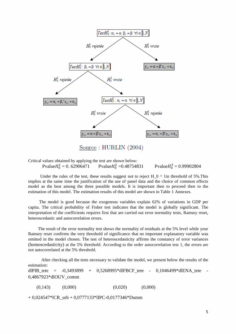
According Hurlin (2004), the test procedure follows the logic defined via the following tree:
5
Critical values obtained by applying the test are shown below:
Pvalue = 0. 62906471 Pvalue
=0.48754831 Pvalue = 0.99902804
Under the rules of the test, these results suggest not to reject H_0 ^ 1in threshold of 5%.This implies at the same time the justification of the use of panel data and the choice of common effects model as the best among the three possible models. It is important then to proceed then to the
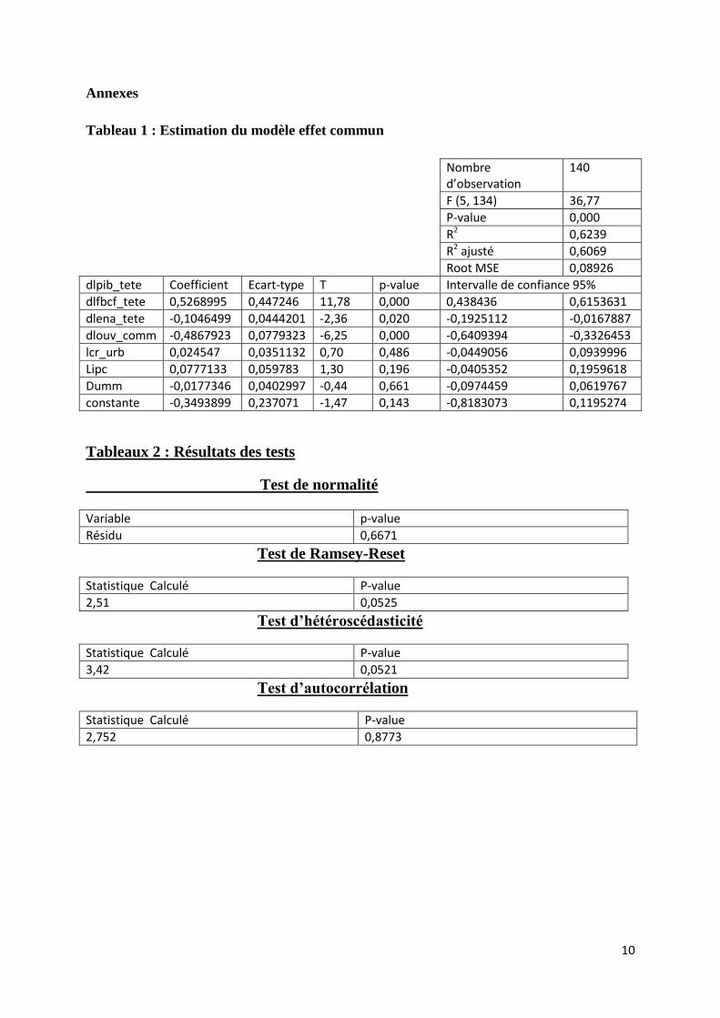
estimation of this model. The estimation results of this model are shown in Table 1 Annexes.
The model is good because the exogenous variables explain 62% of variations in GDP per
capita. The critical probability of Fisher test indicates that the model is globally significant. The
interpretation of the coefficients requires first that are carried out error normality tests, Ramsey reset,
heteroscedastic and autocorrelation errors.
The result of the error normality test shows the normality of residuals at the 5% level while your Ramsey reset confirms the very threshold of significance that no important explanatory variable was
omitted in the model chosen. The test of heteroscedasticity affirms the constancy of error variances
(homoscedasticity) at the 5% threshold. According to the order autocorrelation test 1, the errors are
not autocorrelated at the 5% threshold.
After checking all the tests necessary to validate the model, we present below the results of the
estimation:
dlPIB_tete = -0,3493899 + 0,5268995*dlFBCF_tete - 0,1046499*dlENA_tete -
0,4867923*dlOUV_comm
(0,143) (0,000) (0,020) (0,000)
+ 0,024547*lCR_urb + 0,0777133*lIPC-0,0177346*Dumm
6
(0,486) (0,196) (0,661)
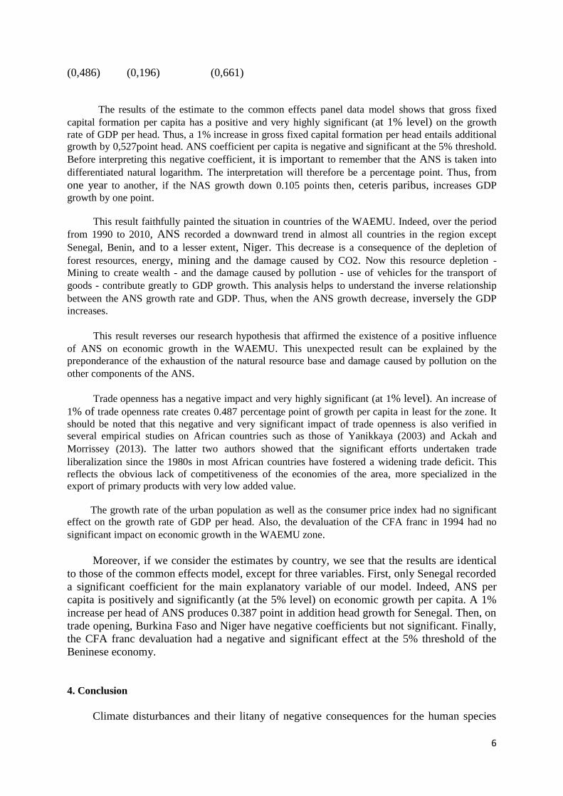
The results of the estimate to the common effects panel data model shows that gross fixed
capital formation per capita has a positive and very highly significant (at 1% level) on the growth
rate of GDP per head. Thus, a 1% increase in gross fixed capital formation per head entails additional
growth by 0,527point head. ANS coefficient per capita is negative and significant at the 5% threshold. Before interpreting this negative coefficient, it is important to remember that the ANS is taken into
differentiated natural logarithm. The interpretation will therefore be a percentage point. Thus, from
one year to another, if the NAS growth down 0.105 points then, ceteris paribus, increases GDP
growth by one point.
This result faithfully painted the situation in countries of the WAEMU. Indeed, over the period from 1990 to 2010, ANS recorded a downward trend in almost all countries in the region except
Senegal, Benin, and to a lesser extent, Niger. This decrease is a consequence of the depletion of
forest resources, energy, mining and the damage caused by CO2. Now this resource depletion - Mining to create wealth - and the damage caused by pollution - use of vehicles for the transport of
goods - contribute greatly to GDP growth. This analysis helps to understand the inverse relationship
between the ANS growth rate and GDP. Thus, when the ANS growth decrease, inversely the GDP increases.
This result reverses our research hypothesis that affirmed the existence of a positive influence of ANS on economic growth in the WAEMU. This unexpected result can be explained by the
preponderance of the exhaustion of the natural resource base and damage caused by pollution on the
other components of the ANS.
Trade openness has a negative impact and very highly significant (at 1% level). An increase of
1% of trade openness rate creates 0.487 percentage point of growth per capita in least for the zone. It should be noted that this negative and very significant impact of trade openness is also verified in
several empirical studies on African countries such as those of Yanikkaya (2003) and Ackah and Morrissey (2013). The latter two authors showed that the significant efforts undertaken trade
liberalization since the 1980s in most African countries have fostered a widening trade deficit. This
reflects the obvious lack of competitiveness of the economies of the area, more specialized in the
export of primary products with very low added value.
The growth rate of the urban population as well as the consumer price index had no significant effect on the growth rate of GDP per head. Also, the devaluation of the CFA franc in 1994 had no
significant impact on economic growth in the WAEMU zone.
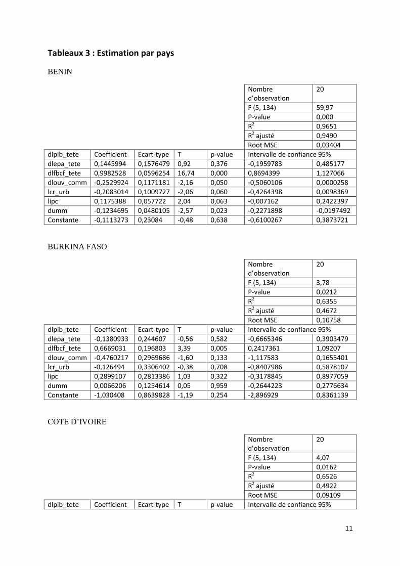
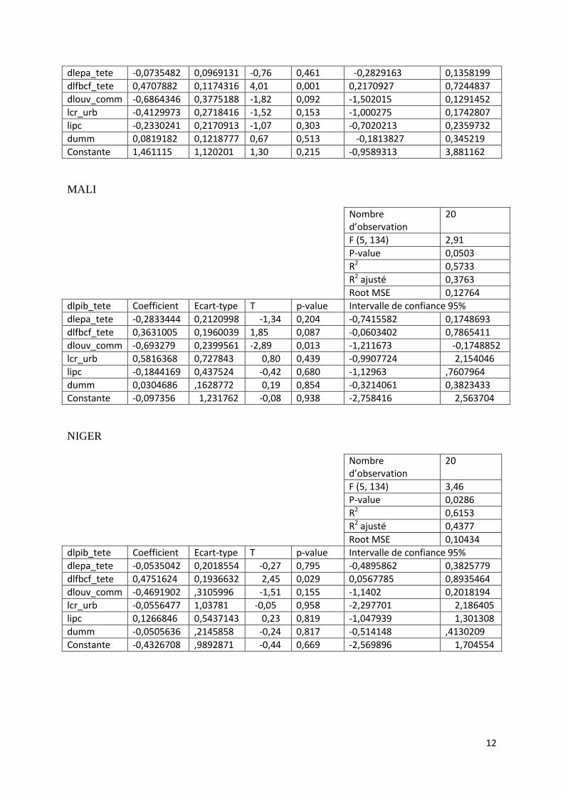
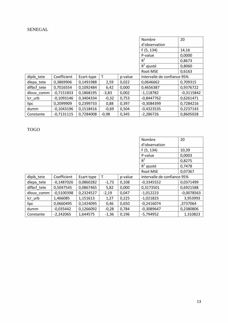
Moreover, if we consider the estimates by country, we see that the results are identical
to those of the common effects model, except for three variables. First, only Senegal recorded
a significant coefficient for the main explanatory variable of our model. Indeed, ANS per
capita is positively and significantly (at the 5% level) on economic growth per capita. A 1%
increase per head of ANS produces 0.387 point in addition head growth for Senegal. Then, on
trade opening, Burkina Faso and Niger have negative coefficients but not significant. Finally,
the CFA franc devaluation had a negative and significant effect at the 5% threshold of the
Beninese economy.
4. Conclusion
Climate disturbances and their litany of negative consequences for the human species

7
and its ecosystem fostered an awareness of the need for better use of renewable resources and
development that respects nature. It is in this context that the World Bank has developed
ANS, composed of physical capital, human capital and environmental capital. It is a relevant
indicator for assessing the sustainable development level of a country. Measuring the contribution of ANS in economic growth in WAEMU countries is the focus of
this article. The results of the estimation of panel data model for common effects have shown, contrary to the hypothesis originally considered that the ANS has a negative and significant effect at
the 5% threshold on growth in the WAEMU zone. Indeed, the results have rather shown an inverse
relationship between the ENA growth rate and GDP. Thus, when the ENA growth decreases by 0.105 points, the GDP increases by one. The importance of natural resource depletion and damage caused
by pollution in relation to other components of the ENA - net national savings and human capital
accumulation - explains the nature of this relationship. This result also puts implicitly highlight an
unfortunate reality in environmental policy in the UEMOA area.
The results also revealed positive and significant role at the 1% of GFCF on economic growth
rates of the UEMOA. Thus, a 1% increase in GFCF per capita growth generates additional head 0.527 points.
The implications of these results in terms of economic policy for WAEMU countries can
be summarized in four points. First, the BCEAO should ease monetary conditions to further
promote private investment and increasing the ANS through its physical component. Then the
eurozone countries have interest in adopting a more sober behavior for operating expenses to
increase the volume of their net savings. Then, at Community level, states could encourage,
through targeted and appropriate tax incentives, companies based in the sub-region to adopt a
more judicious and responsible natural resource management. So it is urgent to take corrective
measures to ensure that the increase in the income of a eurozone countries may be
accompanied by investment in physical capital can compensate for the depletion of natural
resources. Finally, each member state would do well to substantially increase spending on
education to promote human capital essential component of ANS.

8
REFERENCES
Ackah, C., Morrissey, O., 2013, « Trade Policy and Performance in Sub-Saharan Africa Since
The 1980s », CREDIT Research Paper, No. 05/13, Centre for Research in
EconomicDevelopment and International Trade, University of Nottingham, 46 p.
Adjakidje D. et EbongEnone M. (2011), « Impact de la croissance urbaine sur la croissance
économique en Afrique au sud du Sahara : une analyse en données de panel. », Colloque
Dynamiques de croissance au sein de l’Union Economique et Monétaire Ouest Africaine
(UEMOA)’, Ouagadougou, juillet, 23 p.
Agbahoungbata, C. T. S., Dieng, S. A. (2014), « Financement des économies de l’UEMOA :
une analyse en termes de causalité, entre l’aide publique au développement, l’épargne
véritable et la croissance économique », Working Paper, LAREM, n° 16, 34 p.
Asheim, G. B., Weitzman, M. L., (2001). « Does NNP growth indicate welfare improvement
? », Economics Letters, 73, pp. 233–239.
Atkinson, G., Hamilton K. (2003), « Saving, growth and the resource curse hypothesis »,
World Development, pp. 1793-1807.
Atkinson, G., Hamilton, K. (2007), Progress along the path : evolving issues in the
measurement of genuine saving, Environmental and Resource Economics, P. 43-61.
Banque mondiale (1999)
Bruntland, G. H. (1987). « Notre avenir à tous», Commission mondiale sur l’environnement
et le développement, version française, Editions du Fleuve, 349 p.
Dasgupta, P., Heal, M. G. (1974). « The optimal depletion of exhaustible resources », Review
of economic studies, 41 (S), pp. 3-28.
Dasgupta, P., Mäler, K.-G. (2000). « Net national product, wealth, and social well-being »,
Environment and Development Economics, 5, pp. 69-93.
IPCC (GIEC). (2015). « climate Change 2014, Synthesis Report», WMO, UNEP, 169 p.
Hamilton, C. (2007). Measuring sustainable economic welfare : in Atkinson, G., Dietz, S.,
Hamilton, K. (1995). GNP and genuine savings, Centre for Social and Economic Research on
the Global Environment (CSERGE), University College London and University of East
Anglia, London.
Hamilton, K., Clemens, M. (1999),« Genuine savings rates in developing countries », The
World Bank Economic Review, 13, no. 2, pp. 333–56.
Hartwick, J. M. (1977), « Intergenerational Equity and the Investing of Rents from
Exhaustible Resources », The American Economic Review, Vol. 67, No. 5, pp. 972-974.
9
Hurlin, C., 2004, Testing Granger Causality in Heterogeneous Panel Data Models with Fixed
Coe¢ cients. Document de recherche LEO.
Institut pour un développement durable (IDD) (2001), « Qu’est-ce que l’épargne véritable ? »,
in Indicateurs pour un développement durable, N°01-1, Janvier-février 2001, 3p.
Koopmans, T. C. (1965), « On the Concept of Optimal Economie Growth », The econometric
approach to development planning, PontificiaeAcademiaeScientiarumScriptaVaria, P. 225-
287.
Kuznets S. (1955), Economic growth and income inequality, American Economic Review,
vol 49, P. 1-28.
Levin, A., C.-F. Lin, and C.-S. J. Chu., 2002, Unit root tests in panel data: Asymptotic and
finite-sample properties, Journal of Econometrics 108: 1–24.
Mankiw, G., Romer, D. et Weil, D. (1992), A Contribution to the Empirics of Economic
Growth, Quarterly Journal of Economics, 107, P. 407-437.
Ngégné, Y. (2010), « Le développement soutenable : Quatre essais sur l’épargne nette ajustée
et la mesure du développement soutenable », Thèse Nouveau Régime, CERDI, Université
d’Auvergne Clermont-Ferrand I, 177 p.
Pillarisetti, J.R. et Bergh, V. D. J. (2008), Sustainable Nations : What do Aggregate Indicators
Tell Us ?, In Tinbergen Institute Discussion Paper, N° 012/3.
PNUD (2014). Rapport sur le développement humain, 2014, 259 p.
Ramsey, J. B., 1969, "Test for Specification error in Classical Linear Least Squares
Regression Analysis," Journal of the Royal Statistical Society, Series B. 31, 350-371.
Stiglitz, J., 1974, « Growth with Exhaustible Natural Resources : Efficient and Optimal
Growth Paths », The Review of Economic Studies, 41, pp. 123-137.
Yanikkaya, H., 2003, « Trade openness and economicgrowth : a cross-country empirical
investigation», Journal of DevelopmentEconomics, 72, pp. 57–89.
10
Annexes
Tableau 1 : Estimation du modèle effet commun
Nombre d’observation
140
F (5, 134) 36,77
P-value 0,000
R2 0,6239
R2 ajusté 0,6069
Root MSE 0,08926
dlpib_tete Coefficient Ecart-type T p-value Intervalle de confiance 95%
dlfbcf_tete 0,5268995 0,447246 11,78 0,000 0,438436 0,6153631
dlena_tete -0,1046499 0,0444201 -2,36 0,020 -0,1925112 -0,0167887
dlouv_comm -0,4867923 0,0779323 -6,25 0,000 -0,6409394 -0,3326453
lcr_urb 0,024547 0,0351132 0,70 0,486 -0,0449056 0,0939996
Lipc 0,0777133 0,059783 1,30 0,196 -0,0405352 0,1959618
Dumm -0,0177346 0,0402997 -0,44 0,661 -0,0974459 0,0619767
constante -0,3493899 0,237071 -1,47 0,143 -0,8183073 0,1195274
Tableaux 2 : Résultats des tests
Test de normalité
Test de Ramsey-Reset
Statistique Calculé P-value
2,51 0,0525
Test d’hétéroscédasticité
Statistique Calculé P-value
3,42 0,0521
Test d’autocorrélation
Statistique Calculé P-value
2,752 0,8773
Variable p-value
Résidu 0,6671
11
Tableaux 3 : Estimation par pays
BENIN
Nombre d’observation
20
F (5, 134) 59,97
P-value 0,000
R2 0,9651
R2 ajusté 0,9490
Root MSE 0,03404
dlpib_tete Coefficient Ecart-type T p-value Intervalle de confiance 95%
dlepa_tete 0,1445994 0,1576479 0,92 0,376 -0,1959783 0,485177
dlfbcf_tete 0,9982528 0,0596254 16,74 0,000 0,8694399 1,127066
dlouv_comm -0,2529924 0,1171181 -2,16 0,050 -0,5060106 0,0000258
lcr_urb -0,2083014 0,1009727 -2,06 0,060 -0,4264398 0,0098369
lipc 0,1175388 0,057722 2,04 0,063 -0,007162 0,2422397
dumm -0,1234695 0,0480105 -2,57 0,023 -0,2271898 -0,0197492
Constante -0,1113273 0,23084 -0,48 0,638 -0,6100267 0,3873721
BURKINA FASO
Nombre d’observation
20
F (5, 134) 3,78
P-value 0,0212
R2 0,6355
R2 ajusté 0,4672
Root MSE 0,10758
dlpib_tete Coefficient Ecart-type T p-value Intervalle de confiance 95%
dlepa_tete -0,1380933 0,244607 -0,56 0,582 -0,6665346 0,3903479
dlfbcf_tete 0,6669031 0,196803 3,39 0,005 0,2417361 1,09207
dlouv_comm -0,4760217 0,2969686 -1,60 0,133 -1,117583 0,1655401
lcr_urb -0,126494 0,3306402 -0,38 0,708 -0,8407986 0,5878107
lipc 0,2899107 0,2813386 1,03 0,322 -0,3178845 0,8977059
dumm 0,0066206 0,1254614 0,05 0,959 -0,2644223 0,2776634
Constante -1,030408 0,8639828 -1,19 0,254 -2,896929 0,8361139
COTE D’IVOIRE
Nombre d’observation
20
F (5, 134) 4,07
P-value 0,0162
R2 0,6526
R2 ajusté 0,4922
Root MSE 0,09109
dlpib_tete Coefficient Ecart-type T p-value Intervalle de confiance 95%
12
dlepa_tete -0,0735482 0,0969131 -0,76 0,461 -0,2829163 0,1358199
dlfbcf_tete 0,4707882 0,1174316 4,01 0,001 0,2170927 0,7244837
dlouv_comm -0,6864346 0,3775188 -1,82 0,092 -1,502015 0,1291452
lcr_urb -0,4129973 0,2718416 -1,52 0,153 -1,000275 0,1742807
lipc -0,2330241 0,2170913 -1,07 0,303 -0,7020213 0,2359732
dumm 0,0819182 0,1218777 0,67 0,513 -0,1813827 0,345219
Constante 1,461115 1,120201 1,30 0,215 -0,9589313 3,881162
MALI
Nombre d’observation
20
F (5, 134) 2,91
P-value 0,0503
R2 0,5733
R2 ajusté 0,3763
Root MSE 0,12764
dlpib_tete Coefficient Ecart-type T p-value Intervalle de confiance 95%
dlepa_tete -0,2833444 0,2120998 -1,34 0,204 -0,7415582 0,1748693
dlfbcf_tete 0,3631005 0,1960039 1,85 0,087 -0,0603402 0,7865411
dlouv_comm -0,693279 0,2399561 -2,89 0,013 -1,211673 -0,1748852
lcr_urb 0,5816368 0,727843 0,80 0,439 -0,9907724 2,154046
lipc -0,1844169 0,437524 -0,42 0,680 -1,12963 ,7607964
dumm 0,0304686 ,1628772 0,19 0,854 -0,3214061 0,3823433
Constante -0,097356 1,231762 -0,08 0,938 -2,758416 2,563704
NIGER
Nombre d’observation
20
F (5, 134) 3,46
P-value 0,0286
R2 0,6153
R2 ajusté 0,4377
Root MSE 0,10434
dlpib_tete Coefficient Ecart-type T p-value Intervalle de confiance 95%
dlepa_tete -0,0535042 0,2018554 -0,27 0,795 -0,4895862 0,3825779
dlfbcf_tete 0,4751624 0,1936632 2,45 0,029 0,0567785 0,8935464
dlouv_comm -0,4691902 ,3105996 -1,51 0,155 -1,1402 0,2018194
lcr_urb -0,0556477 1,03781 -0,05 0,958 -2,297701 2,186405
lipc 0,1266846 0,5437143 0,23 0,819 -1,047939 1,301308
dumm -0,0505636 ,2145858 -0,24 0,817 -0,514148 ,4130209
Constante -0,4326708 ,9892871 -0,44 0,669 -2,569896 1,704554
13
SENEGAL
Nombre d’observation
20
F (5, 134) 14,16
P-value 0,0000
R2 0,8673
R2 ajusté 0,8060
Root MSE 0,6163
dlpib_tete Coefficient Ecart-type T p-value Intervalle de confiance 95%
dlepa_tete 0,3869906 0,1491988 2,59 0,022 0,0646662 0,709315
dlfbcf_tete 0,7016554 0,1092484 6,42 0,000 0,4656387 0,9376722
dlouv_comm -0,7151833 0,1868195 -3,83 0,002 -1,118782 -0,3115842
lcr_urb -0,1093146 0,3404334 -0,32 0,753 -0,8447762 0,6261471
lipc 0,2099909 0,2399733 0,88 0,397 -0,3084399 0,7284216
dumm -0,1043196 0,1518416 -0,69 0,504 -0,4323535 0,2237143
Constante -0,7131115 0,7284008 -0,98 0,345 -2,286726 0,8605028
TOGO
Nombre d’observation
20
F (5, 134) 10,39
P-value 0,0003
R2 0,8275
R2 ajusté 0,7478
Root MSE 0,07367
dlpib_tete Coefficient Ecart-type T p-value Intervalle de confiance 95%
dlepa_tete -0,1487026 0,0860282 -1,73 0,108 -0,3345552 0,0371499
dlfbcf_tete 0,5047545 0,0867465 5,82 0,000 0,3173501 0,6921588
dlouv_comm -0,5100398 0,2324527 -2,19 0,047 -1,012223 -0,0078563
lcr_urb 1,466085 1,151613 1,27 0,225 -1,021823 3,953993
lipc 0,0660495 0,1424095 0,46 0,650 -0,2416074 ,3737064
dumm -0,035442 0,1266092 -0,28 0,784 -0,3089647 0,2380806
Constante -2,242065 1,644575 -1,36 0,196 -5,794952 1,310823


