Download - Adjoint Based Anisotropic Mesh Adaptation for the CPR …dept.ku.edu/~cfdku/papers/AIAA-2013-2869.pdf · Adjoint Based Anisotropic Mesh Adaptation for the ... 10.2514/6.2013-2869

Adjoint Based Anisotropic Mesh Adaptation for the

CPR Method

Lei Shi∗ and Z.J. Wang †

Department of Aerospace Engineering, University of Kansas, Lawrence, KS, 66045

Adjoint-based adaptive methods have the capability of dynamically distributing comput-ing power to areas which are important for predicting an engineering output such as lift ordrag. In this paper, we apply an anisotropic h-adaptation method for simplex meshes usingthe correction procedure via reconstruction(CPR) method with the target of minimizingthe output error. An adjoint-based error estimation with a local refinement sampling pro-cess is utilized to drive the anisotropic mesh refinement without making any assumptionabout the solution features. The accuracy and efficiency of the isotropic and anisotropicadaptation strategies are compared on several 2D inviscid flow problems.

I. Introduction

High order methods have the potential of delivering higher accuracy with less CPU time than lower ordermethods. However, for a compact scheme, the number of degrees of freedom (DOF) rises rapidly with

the increased order of accuracy, which affects the prevalence of high-order methods in industry applications.Solution based adaptive methods has the capability of dynamically distributing computing power to a desiredarea to achieve required accuracy with minimal costs.[1–3] For this reason, adaptive high-order methods havereceived considerable attention in the high-order CFD community. [4–9].

The truncation error of a spatial discretization is determined by the mesh size and the order of thepolynomial approximation. P-adaptations can be applied to smooth regions while h-adaptations are preferredfor shock waves or singularities[10, 11]. The discretization of a compact scheme only depends on a small stencilof local DOFs. This compact support simplifies the task of hp-adaptations involving complex geometries.Several compact high-order methods for unstructured meshes have been developed, such as the discontinuousGalerkin(DG) method [10, 12, 13], the spectral volume (SV) method [14, 15] and the spectral difference (SD)method [16]. Unlike the finite volume method that achieves high-order by expanding their reconstructionstencil, the above methods employ local DOFs to support high-order piecewise solution polynomials in eachelement, and the interaction between the local cell and its neighbors is provided by the common flux at theboundary. Recently, the flux reconstruction or the correction procedure via reconstruction (CPR) formulationwas developed in 1D [17], and further extended in Ref. [18–23]. It is a nodal differential formulation whichcan unite several well known high-order methods such as DG, SV and SD. The CPR formulation combinesthe compactness and high accuracy with the simplicity and efficiency of the finite difference method, andcan be easily implemented for mixed unstructured meshes.

The effectiveness of adaptation methods highly depends on the accuracy of error estimations. There areat least three major types of adaptation criteria: gradient or feature based [24–27], residual-based [28–33],and adjoint-based [4–8, 34–42]. Heuristic feature-based criterion such as large gradient cannot provide anuniversal and robust error estimation [5, 43]. The residual-based error indicator which is defined locallyon each element has had some successes; however, it can lead to false refinements in convection-dominatedflow. Adjoint-based error estimations relates a specific functional output directly to the local residual bysolving an additional adjoint problem, and is gaining a lot of research attention, which relates a specificfunctional output directly to the local residual by solving an additional adjoint problem. It can capturethe propagation effects inherent in hyperbolic equations and has been shown very effective in driving an

∗PhD Student, Department of Aerospace Engineering, 2120 Learned Hall, Lawrence, KS 66045, AIAA Member.†Spahr Professor and Chair, Department of Aerospace Engineering, 2120 Learned Hall, Lawrence, KS 66045, Associate

Fellow of AIAA.

1 of 18

American Institute of Aeronautics and Astronautics

Dow

nloa

ded

by U

NIV

ER

SIT

Y O

F K

AN

SAS

on J

uly

1, 2

013

| http

://ar

c.ai

aa.o

rg |

DO

I: 1

0.25

14/6

.201

3-28

69

21st AIAA Computational Fluid Dynamics Conference

June 24-27, 2013, San Diego, CA

AIAA 2013-2869

Copyright © 2013 by the American Institute of Aeronautics and Astronautics, Inc. All rights reserved.

hp-adaptation procedure to obtain a very accurate prediction of the functional output. Recently Fidkowskiand P.L Roe developed a new error indicator based on the entropy variables to drive an hp-adaptation forinviscid and viscous flow. Entropy variables can be interpreted as the dual solution for the output of entropybalance in the whole domain. It can be obtained directly from the state variables without solving extraadjoint equations.[44, 45]

Compressible viscous flow may produce strong directional phenomena, such as boundary layers, shearlayers and shock waves. For isotropic adaptation, each cell is subdivided into four elements in 2D and eightelements in 3D, which is very costly to resolve these behaviors. In contrast, stretched elements with highaspect ratio are preferred for optimal resolution of anisotropic features. Considerable work has been devotedto the adjoint based anisotropic adaptation. A common and simple approach to incorporate the directionalinformation for adaptation is to use the Hessian-based metric field of a solution variable, which representsthe interpolation error[2, 46]. However, it does not provide any information for the functional error. Vendittiand Darmofal [5] have extended the Hessian-based metric of the Mach number to the dual weighted metricswith size information. While similar techniques have been applied in the Ref. [3, 7, 47–49], their anisotropydecision requires a priori knowledge of the solution. Furthermore, the directional information does notdirectly relate to the functional error. Recently, a popular approach to drive anisotropic adaptation is toperform a output error sampling procedure from a discrete set of refinement choices. The idea of guidinganisotropy adaptation for the engineering output by solving local problems has been previously proposedin the Ref. [39, 41, 42, 50]. During the trial refinements process, the elemental functional error is directlyestimated and monitored. In this paper, we use this sampling procedure to drive the anisotropic adaptation.

The adjoint solution is particularly important for the error estimation and output-based adaptation.There are two approaches to obtain the adjoint solution for primal problems. We can solve the continuousadjoint equation which is a partial differential equation using any numerical method or directly solve thediscrete adjoint equation derived from the discretized primal equation. It has been shown that the discreteadjoint solution leads to a more accurate error estimation for the fine grid functional, while continuousadjoints gives better output estimation when the primal and adjoint solutions are well resolved [51]. However,the discrete adjoint solution should be consistent with the exact adjoint from the continuous adjoint equation.It is well known that the dual consistency can significantly impact the convergence of both the primal andadjoint approximations. There are several possible sources of dual inconsistency that can be introduced intoa high-order discretization. A dual consistent discretization with semilinear forms such as the finite elementand DG methods have been well examined for the Euler and Navier-Stokes equations [34, 37, 52, 53].However, the analysis of dual consistency for differential-type methods has not been well investigated, whichis one of the focuses of the present paper.

The rest of the paper is organized as follows: In section 2 we briefly review the high-order CPR method.The continuous and discrete adjoint equations and the dual consistent discretization of the CPR method aredescribed in Section 3. Then section 4 presents adaptation strategies and procedures for hp-adaptations.Finally, several numerical test cases are presented in Section 5, and conclusions are given in section 6.

II. Review of the CPR Method

For the sake of completeness, the CPR formulation is briefly reviewed. The CPR formulation wasoriginally developed by Huynh in Ref. [17, 54] under the name of flux reconstruction, and extended tosimplex and hybrid elements by Wang & Gao in Ref. [18] under lifting collocation penalty. In Ref. [55], CPRwas further extended to 3D hybrid meshes. The method is also described in two book chapters [56]. CPRcan be derived from a weighted residual method by transforming the integral formulation into a differentialone. First, a hyperbolic conservation law can be written as

∂Q

∂t+∇ · ~F(Q) = 0 (1)

with proper initial and boundary conditions, where Q is the state vector, and ~F (F,G) is the flux vector.Assume that the computational domain Ω is discretized into N non-overlapping triangular elements ViNi=1

Let W be an arbitrary weighting function or test function. The weighted residual formulation of Eq. (1) onelement Vi can be expressed as ∫

Vi

(∂Q

∂t+∇ · ~F(Q))W dV = 0. (2)

2 of 18


Dow

nloa

ded

by U

NIV

ER

SIT

Y O

F K

AN

SAS

on J

uly

1, 2

013

| http

://ar

c.ai

aa.o

rg |

DO

I: 1

0.25

14/6

.201

3-28

69


After applying integration by parts to the flux divergence, we can get∫Vi

∂Q

∂tW dV +

∫∂Vi

W ~F(Q) · ~ndS −∫Vi

∇W · ~F(Q) dV = 0. (3)

Let Qi be an approximate solution to the analytical solution Q on Vi. On each element, the solution belongsto the space of polynomials of degree k or less, i.e., Qi ∈ P k(Vi) (or P k if there is no confusion) with nocontinuity requirement across element interfaces. Let the dimension of P k be K = (k + 1)(k + 2)/2. Inaddition, the numerical solution Qi , for the moment, is required to satisfy Eq. (3) as∫

Vi

∂Qi∂t

W dV +

∫∂Vi

W ~F(Qi) · ~ndS −∫Vi

∇W · ~F(Qi) dV = 0. (4)

Obviously the surface integral is not properly defined because the numerical solution is discontinuous acrosselement interfaces. Following the idea used in the Godunov method [57, 58], the normal flux term in Eq. (4)is replaced with a common Riemann flux, e.g., in Ref. [59–61]

Fn(Qi) ≡ ~F(Qi) · ~n ≈ Fncom(Qi, Qi+, ~n), (5)

where Qi+ denotes the solution outside the current element Vi. Instead of Eq. (4), the approximate solutionis required to satisfy ∫

Vi

∂Qi∂t

W dV +

∫∂Vi

WFncom dS −∫Vi

∇W · ~F(Qi) dV = 0. (6)

Applying integration by parts again to the last term of the above LHS, we obtain∫Vi

∂Qi∂t

W dV +

∫Vi

W∇ · ~F(Qi) dV +

∫∂Vi

W [Fncom −Fn(Qi)] dS = 0. (7)

Here, the test space has the same dimension as the solution space, and is chosen in a manner to guaranteethe existence and uniqueness of the numerical solution.

Note that the quantity ∇ · ~F(Qi) involves no influence from the data in the neighboring cells. Theinteraction between the current cell and its neighbors is represented by the above boundary integral, whichis also called a penalty term, penalizing the normal flux differences.

The next step is critical in the elimination of the test function. The boundary integral above is cast as avolume integral via the introduction of a correction field on Vi, δi ∈ P k(Vi),∫

Vi

Wδi dV =

∫∂Vi

W [Fn] dS, (8)

where [Fn] = Fncom − Fn(Qi) is the normal flux difference. The above equation is sometimes referred to asthe lifting operator, which has the normal flux differences on the boundary as input and a member of P k(Vi)as output. Substituting Eq. (8) into Eq. (7), we obtain∫

Vi

(∂Qi∂t

+∇ · ~F(Qi) + δi)W dV = 0. (9)

If the flux vector is a linear function of the state variable, then ∇· ~F(Qi) ∈ P k. In this case, the terms insidethe square bracket are all elements of P k . Because the test space is selected to ensure a unique solution,Eq. (9) is equivalent to

∂Qi∂t

+∇ · ~F(Qi) + δi = 0. (10)

For nonlinear conservation laws, ∇ · ~F(Qi) is usually not an element of P k. As a result, Eq. (9) cannot

be reduced to Eq. (10). In this case, the most obviously choice is to project ∇ · ~F(Qi) into P k. Denote

Π(∇ · ~F(Qi)) as a projection of ∇ · ~F(Qi) to P k. One choice is∫Vi

Π(∇ · ~F(Qi))W dV =

∫Vi

∇ · ~F(Qi)W dV. (11)

3 of 18


Dow

nloa

ded

by U

NIV

ER

SIT

Y O

F K

AN

SAS

on J

uly

1, 2

013

| http

://ar

c.ai

aa.o

rg |

DO

I: 1

0.25

14/6

.201

3-28

69


Then Eq. (9) reduces to∂Qi∂t

+ Π(∇ · ~F(Qi)) + δi = 0. (12)

With the introduction of the correction field δi, and a projection of ∇· ~F(Qi) for nonlinear conservation laws,we have reduced the weighted residual formulation to a differential formulation, which involves no explicitintegrals. Note that for δi defined by Eq. (8), if W ∈ P k, Eq. (12) is equivalent to the DG formulation, atleast for linear conservation laws; if W belongs to another space, the resulting δi is different. We obtain aformulation corresponding to a different method such as the SV method.

Next, let the DOFs be the solutions at a set of solution points (SPs) ~ri,j (j varies from 1 to K), asshown in Figure 1. Then Eq. (12) holds true at the SPs, i.e.,

∂Qi,j∂t

+ Πj(∇ · ~F(Qi)) + δi,j = 0, (13)

where Πj(∇ · ~F(Qi)) denotes the values of Π(∇ · ~F(Qi)) at SP j. The efficiency of the CPR approach hinges

on how the correction field δi and the projection Π(∇ · ~F(Qi)) are computed. Two approaches can be usedto compute this divergence as detailed in Ref. [18]. To compute δi, we define k+1 points named flux points

Figure 1. Gaussian solution points(SP) and flux points(FP) for k=2 (©-SP ,a

-FP)

(FPs) along each interface, where the normal flux differences are computed, as shown in Figure 1. Weapproximate (for nonlinear conservation laws) the normal flux difference [Fn] with a degree k interpolationpolynomial along each interface

[Fn]f ≈ Ik[Fn]f ≡∑l

[Fn]f,lLFPl , (14)

where f is a face (or edge in 2D) index, and l is the FP index, and LFPl is the Lagrange interpolationpolynomial based on the FPs in a local interface coordinate. For linear triangles with straight edges, oncethe solution points and flux points are chosen, the correction at the SPs can be written as

δi,j =1

|Vi|∑f∈∂Vi

∑l

αj,f,l[Fn]f,lSf , (15)

where αj,f,l are lifting constants independent of the solution variables, Sf is the face area, |Vi| is the volumeof Vi. Note that the correction for each solution point, namely δi,j , is a linear combination of all the normalflux differences on all the faces of the cell. Conversely, a normal flux difference at a flux point on a face, say(f,l) results in a correction at all solution points j of an amount αj,f,l[Fn]f,lSf/|Vi|.

III. Adjoint-Based Error Estimation

III.A. The Continuous Adjoint Equation

Adjoint-based error estimation can directly relate the local residual error from the primal equation to theengineering output. The accuracy of adjoint solution is particularly important for accurate error estimation.There are two approaches to obtain the adjoint solution. We can solve the continuous adjoint equation which

4 of 18


Dow

nloa

ded

by U

NIV

ER

SIT

Y O

F K

AN

SAS

on J

uly

1, 2

013

| http

://ar

c.ai

aa.o

rg |

DO

I: 1

0.25

14/6

.201

3-28

69


is a partial differential equation using any numerical method or directly solve the discrete adjoint equationderived from the discretized primal equation. As for the primal problem, a numerical scheme is defined as aconsistent method if its discrete operator converges to the continuous operator, or the exact solution couldsatisfy the discrete numerical formulation as the mesh size approach to zero. Similarly, dual-consistency isdefined as the exact adjoint solution from the continuous adjoint equation should satisfy the discrete adjointequation. In order to analyze the dual consistency of the CPR method, we need to derive the continuousadjoint equation and its boundary conditions first. Consider a primal differential equation as a conservationlaw

N (Q) = ∇ · ~F(Q) = 0. (16)

Given a scalar output J (Q) of interest, which may consist of surface (∂Ω) and volume (Ω) integration ingeneral as

J (Q) =

∫Ω

JΩ(Q) dΩ +

∫∂Ω

Jτ (Q) ds. (17)

We can define a Lagrangian of the output with the constraint of the solution Q satisfies the primal equationN (Q) = 0, which leads to

L = J (Q) +

∫Ω

ψTN (Q) dΩ. (18)

Here ψ is the adjoint solution, furthermore, it also serves as a Lagrangian multiplier [45, 62]. Let the Frechetlinearization with respect to an argument in the square bracket defined as

J ′[Q](δQ) = J (Q+ δQ)− J (Q) = δJ =∂J∂Q

δQ. (19)

After enforcing stationary of L to a permissible variation δQ, which is belong to the space of permissiblestate variations δQ ∈ Vperm, Eq. (18) yields the linearized Lagrangian or the adjoint equation

L′[Q](δQ) = J ′[Q](δQ) +

∫Ω

ψTN ′[Q](δQ) dΩ = 0 ∀δQ ∈ Vperm. (20)

Plug the definition of Frechet linearization into the above equation, the adjoint Eq. (20) can be expressed as

(∂J∂Q

+

∫Ω

ψT∂N (Q)

∂QdΩ) δQ = 0. (21)

After substituting the definition of the output J and the primal differential equation N (Q) in the adjointEq. (21)

(

∫Ω

∂JΩ

∂QdΩ +

∫∂Ω

∂Jτ∂Q

ds+

∫Ω

ψT∂

∂xi

∂Fi∂Q

dΩ) δQ = 0, (22)

then performing integration by parts leads to

[

∫Ω

(∂JΩ

∂Q− ∂ψT

∂xi

∂Fi∂Q

) dΩ] δQ+ [

∫∂Ω

(∂Jτ∂Q

+ ψT∂Fi∂Q

ni) ds] δQ = 0. (23)

Most of time, the output J only consists of boundary integrations, which means JΩ = 0, so the aboveequation yields the governing equation for the continuous adjoint

∂Fi∂Q

T ∂ψ

∂xi= 0, (24)

and the corresponding boundary conditions defined as

[

∫∂Ω

(∂Jτ∂Q

ds+ ψT∂Fi∂Q

ni) ds] δQ = 0 ∀δQ ∈ Vperm. (25)

The continuous adjoint equation is a linear partial differential equation which can be solved using anynumerical method. An adjoint solution can be used to perform error estimation for an engineering output.First the output error is defined as the difference between the functional evaluated with the analytical solution

5 of 18


Dow

nloa

ded

by U

NIV

ER

SIT

Y O

F K

AN

SAS

on J

uly

1, 2

013

| http

://ar

c.ai

aa.o

rg |

DO

I: 1

0.25

14/6

.201

3-28

69


Q and the discrete numerical solution Qh, which can be further approximated using a linear analysis afterdropping the high order terms as

δJ = J (Qh)− J (Q) ≈ J ′[Q](δQ). (26)

With Eq. (20), the output error can also be expressed as

δJ ≈ J ′[Q](δQ) = −∫

Ω

ψTN ′[Q](δQ) dΩ. (27)

Here, N ′[Q](δQ) is the residual error for the primal problem induced by the primal discretization δQ = Q−Qh

δN = N (Qh)−N (Q) = N (Qh) ≈ N ′[Q](δQ). (28)

So we can express the output error in the form of the adjoint solution weighted with the primal residual

δJ = −∫

Ω

ψTN (Qh) dΩ. (29)

III.B. The Discrete Adjoint Equation

As shown in the previous session, the continuous adjoint equation is a partial differential equation, which isderived directly from the linearized primal equation and the linearized functional outputs. Obviously, thenumerical scheme for the continuous adjoint equation and the primal governing equation can be different. Forthe discrete adjoint approach, the discrete adjoint equation is directly result from linearizing the discretizedprimal equation. In this session, discrete adjoint formulations for schemes with a variational form anddifferential-type schemes are presented and their difference are compared.

For the fully discrete formulation, we need to consider two approximation levels. Here, H stands for acoarse level and h denotes as a fine level. In practise, the coarse and fine levels of the approximation can beachieved using h-refinement or p-enrichment. The output error between those two different approximationscan be denoted as

δJh = Jh(QH)− Jh(Qh). (30)

Our target is to estimate the output Jh(Qh) at fine level without solving the primal solution on the finespace. With the Taylor expansion, the output Jh(Qh) and the residual Rh(Qh) at the fine space h can beexpanded to a prolongated fine solution QHh from a coarse solution QH

Jh(Qh) = Jh(QHh ) +∂Jh∂Qh

|QHh

(Qh −QHh ) + ... (31)

Rh(Qh) = Rh(QHh ) +∂Rh∂Qh

|QHh

(Qh −QHh ) + ...

with the assumption of Rh(Qh) = 0. The prolongated solution QHh = IHh QH can be obtained using theinjection operator IHh . After dropping high order terms and canceling the solution difference (Qh − QHh )between the truth solution at the fine level and the prolongated solution, the above equation can be writtenas

Jh(Qh) ≈ Jh(QHh )− ∂Jh∂Qh

|QHh

(∂Rh∂Qh

|QHh

)−1︸︷︷︸Rh(QHh ) (32)

≈ Jh(QHh ) + (ψh|QHh

)TRh(QHh )

from where we can define the equation for the discrete adjoint solution ψh as

−(ψh)T∂Rh∂Qh

=∂Jh∂Qh

.

After transposing both sides of the above equation, we can express the fully discrete adjoint equation in thefollowing form

−∂Rh∂Qh

T

ψh =∂Jh∂Qh

T

. (33)

6 of 18


Dow

nloa

ded

by U

NIV

ER

SIT

Y O

F K

AN

SAS

on J

uly

1, 2

013

| http

://ar

c.ai

aa.o

rg |

DO

I: 1

0.25

14/6

.201

3-28

69


For numerical methods with a weak form such as FEM methods or DG methods, after choosing a properbasis , Eq. (33) is equivalent to its variational formulation. Detailed derivations can be found in Ref. [9, 52].The fully discrete adjoint solution for numerical schemes in semilinear form is consistent with the continuousadjoint equation. However, this is not true for numerical schemes in differential form such as the CPRmethod, which does not born with a variational form.

Let r(Q)i,j denotes a pointwise residual of a differential scheme defined at each solution point j of cell i

r(Q)i,j = (~∇ · ~F(Qi))j . (34)

If the CPR method is used for discretizing the primal equation, the pointwise residual ri,j can be expressedas

r(Q)i,j = Π(~∇ · ~F(Qi))j +1

|Vi|∑f∈∂Vi

∑l

αj,f,l[Fn]f,lSf . (35)

Substitute the pointwise residual ri,j arising from a differential scheme, the fully discrete adjoint Eq. (33)can be written as

−∑i

∑j

∂ri,j∂Qk

ψi,j =∂J∂Qk

, (36)

where k is index of total DOFs in the whole domain. However, this approach is not consistent with continuousadjoint equation. If we assume the adjoint solution belongs to the same space of the primal solution andapproximate the adjoint variable ψ of the cell i using the Lagrange basis Lj

ψi =∑j

Ljψi,j . (37)

With the above equation, directly discretizing the continuous adjoint Eq. (21) leads to

−∫

Ω

∂N (Q)

∂Q

T

ψ dΩ =∂J∂Q

T

⇒ −∑i

∑j

∂ri,j∂Qk

ωj |Ji,j |ψi,j =∂J∂Qk

, (38)

where ωj and |Ji,j | are the quadrature weight and the element Jacobian at the solution point j of cell i.

Compared with Eq. (36), the following relation can be derived between the discrete adjoints ψi,j and the

continuous adjoint ψi,jψi,j = ωj |Ji,j |ψi,j . (39)

So the fully discrete adjoint formula for a numerical scheme in differential forms is not consistent withthe continuous adjoint equation. The only difference between them are the quadrature weights ω and cellJacobian |J | at each solution point. The discrete adjoint formula for differential schemes should be derivedin integral form. Alternatively, an explicit weak formulation should be defined for numerical schemes indifferential forms for the purpose of obtaining the discrete adjoint solution only. In the next session, adiscrete adjoint equation in integral form for the CPR method, which is dual consistent with the continuousadjoint, is presented and verified using several numerical tests.

III.C. Numerical Verifications of the Dual Consistent CPR Method

Since there is no variational or weak form of the CPR method, its discrete adjoint equation can be directlyderived from the continuous adjoint equation

−∑i

∑j

∂ri,j∂Qk

ωj |Ji,j |ψi,j =∂J∂Qk

, (40)

which results an integral equation. This integral equation can be interpreted as an explicitly defined varia-tional form for the CPR method, whose purpose is only to find the dual consistent discrete adjoint solution.

7 of 18


Dow

nloa

ded

by U

NIV

ER

SIT

Y O

F K

AN

SAS

on J

uly

1, 2

013

| http

://ar

c.ai

aa.o

rg |

DO

I: 1

0.25

14/6

.201

3-28

69


First, inviscid flow over a NACA 0012 airfoil is utilized to demonstrate the smoothness of the discrete adjointsolution from the dual consistent CPR method. This test case is used in Ref. [9]. The inflow condition is setto be M∞ = 0.4 with an angle of attack of 5. The 3rd order CPR formulation using Gaussian quadraturepoints as solution points and flux points is used to ensure the integration accuracy for solving the discreteadjoint equation in integral forms. The dual solution from the fully discrete adjoint formulation of the CPRmethod is shown in Figure 2(a), which is not dual consistent and has an irregular mosaic like distributionsin every cell. Figure 2(b) shows the adjoint solution from the discrete adjoint equation in integral forms.The adjoint solution looks much more smooth than the fully discrete adjoint. Furthermore the square rootsingularity of adjoint solution with respect to distance from the stagnation streamline introduced in Ref. 34are observed near the leading edge.

(a) The fully discrete adjoint (b) The discrete adjoint in the integral form

Figure 2. The x-momentum component of the lift adjoint for a NACA 0012 airfoil at M∞ = 0.4, α = 5

The problem C1.3(a) of the 1st international workshop on high-order methods is used to further assessthe accuracy of the adjoint-based error estimation with the CPR method. This test case involves subsonicflow over a NACA 0012 airfoil with a free-stream Mach number of M∞ = 0.5 and the angle of attack, α = 2.The output of interest is chosen as the lift of the airfoil. The error in the functional JH(QH) − Jh(Qh) iscomputed using p-enrichment from p = 1 to p = 2 and the effectivity of the error estimation is defined as

ηeH =−(ψh)TRh(QHh )

JH(QH)− Jh(Qh)(41)

Table 1 shows the results with 4 levels of uniformly refined meshes from the high-order workshop. Note thatthe error of the initial lift estimation on the very coarse meshes are kind of large; however, the effectivityindex ηeH approaches unity as the mesh refined.

Table 1. Adjoint-based Error Estimation for the lift of a Sub-sonic NACA 0012 Airfoil at M∞ = 0.5, α = 2

Cells JH(QH)− Jh(Qh) −(ψh)TRh(QHh ) ηeH280 -5.859e-3 -1.103e-2 1.88

1120 -2.638e-3 -4.002e-3 1.52

4480 -8.736e-4 -9.995e-4 1.14

17920 -1.933e-4 -1.988e-4 1.03

In this test case, subsonic inviscid flow over a Gaussian-shaped bump is used to demonstrate the implica-tion of the boundary flux for the discrete adjoint solutions near the walls. Again, 3rd order CPR formulationusing Gaussian quadrature points as the solution points and the flux points is employed. This test case getrid of the influence from geometry singularities and stagnation points, which is first used in Ref. 62. Thechannel has an height of 0.8 unit and a length of 3 unit. The bump geometry is defined as

y = 0.0625e−25x2

(42)

8 of 18


Dow

nloa

ded

by U

NIV

ER

SIT

Y O

F K

AN

SAS

on J

uly

1, 2

013

| http

://ar

c.ai

aa.o

rg |

DO

I: 1

0.25

14/6

.201

3-28

69


and the output is defined as a weighted lift on bump surface

J =

∫bump

p(x, y)nye−50x2

ds. (43)

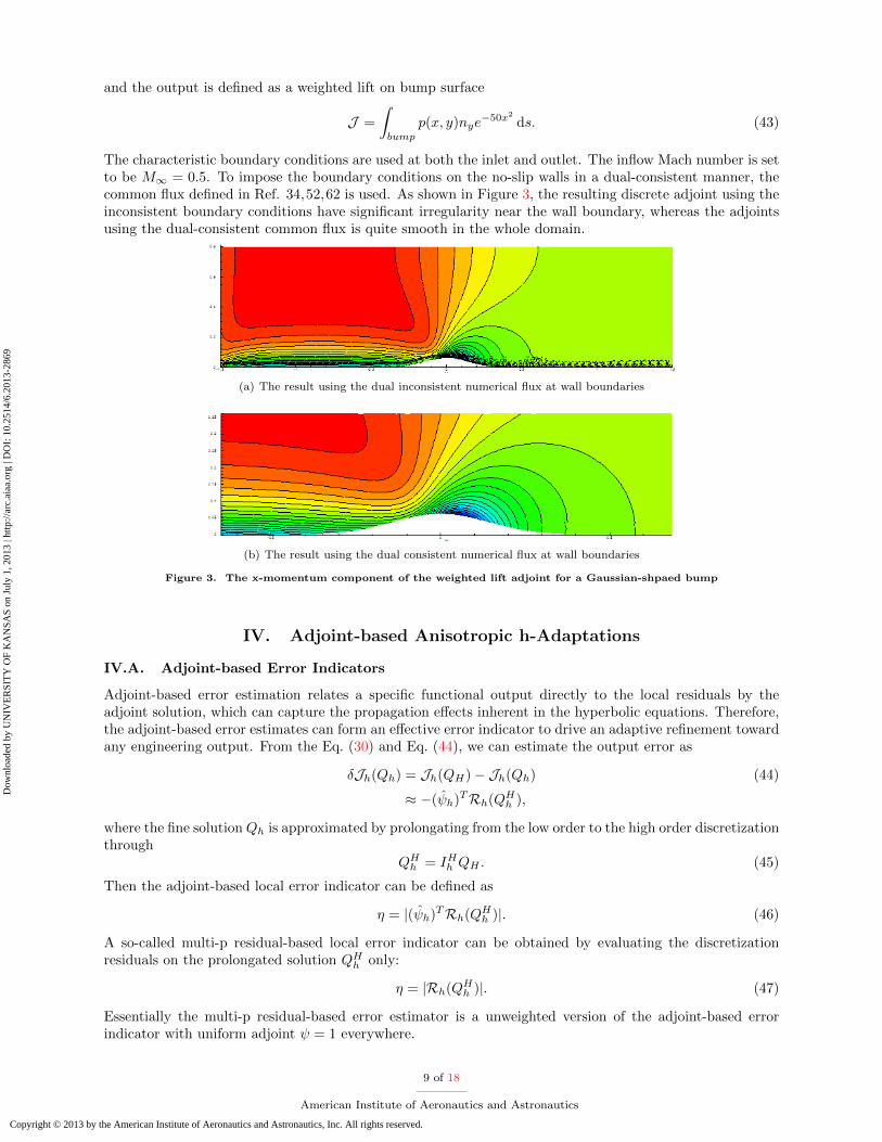
The characteristic boundary conditions are used at both the inlet and outlet. The inflow Mach number is setto be M∞ = 0.5. To impose the boundary conditions on the no-slip walls in a dual-consistent manner, thecommon flux defined in Ref. 34,52,62 is used. As shown in Figure 3, the resulting discrete adjoint using theinconsistent boundary conditions have significant irregularity near the wall boundary, whereas the adjointsusing the dual-consistent common flux is quite smooth in the whole domain.

(a) The result using the dual inconsistent numerical flux at wall boundaries

(b) The result using the dual consistent numerical flux at wall boundaries

Figure 3. The x-momentum component of the weighted lift adjoint for a Gaussian-shpaed bump

IV. Adjoint-based Anisotropic h-Adaptations

IV.A. Adjoint-based Error Indicators

Adjoint-based error estimation relates a specific functional output directly to the local residuals by theadjoint solution, which can capture the propagation effects inherent in the hyperbolic equations. Therefore,the adjoint-based error estimates can form an effective error indicator to drive an adaptive refinement towardany engineering output. From the Eq. (30) and Eq. (44), we can estimate the output error as

δJh(Qh) = Jh(QH)− Jh(Qh) (44)

≈ −(ψh)TRh(QHh ),

where the fine solution Qh is approximated by prolongating from the low order to the high order discretizationthrough

QHh = IHh QH . (45)

Then the adjoint-based local error indicator can be defined as

η = |(ψh)TRh(QHh )|. (46)

A so-called multi-p residual-based local error indicator can be obtained by evaluating the discretizationresiduals on the prolongated solution QHh only:

η = |Rh(QHh )|. (47)

Essentially the multi-p residual-based error estimator is a unweighted version of the adjoint-based errorindicator with uniform adjoint ψ = 1 everywhere.

9 of 18


Dow

nloa

ded

by U

NIV

ER

SIT

Y O

F K

AN

SAS

on J

uly

1, 2

013

| http

://ar

c.ai

aa.o

rg |

DO

I: 1

0.25

14/6

.201

3-28

69


IV.B. Anisotropic h-Adaptations

The error indicators defined above are used to drive a fixed-fraction anisotropic h-adaptation. In thisapproach, a certain fraction f of the current elements with the largest local error indicators η are marked forh-refinements. Then the anisotropic adaptation decision is driven by an error sampling procedure for choosingthe optimal refinement from a discrete set of adaptation choices. The idea of guiding anisotropy adaptationfor the engineering output by solving local problems has been previously proposed in the Ref. [39, 41, 42, 50].The elemental functional error is directly estimated and monitored during the sampling process. For a simplexelement, we consider 4 local refinement options by splitting the edges, as shown in Figure 4.

(a) The original coarse mesh

(b) Isotropic refinement (c) Edge 1 Split (d) Edge 2 Split (e) Edge 3 Split

Figure 4. The simplex refinement options for probing the local functional error behavior

Mesh refinement is performed in the original element’s polynomial space using the reference coordinates.So the refined elements inherit the same geometry approximation order. However, for elements on thegeometry boundaries, the newly generated vertex on the boundary edge may not be exactly on the realgeometry. An extra remapping process is employed to snap the boundary points to the truth geometryduring each adaptation level. As shown in Figure 5, non-conforming interfaces between cells with differenth levels are created during the adaptation process. In order to maintain the smoothness of the solution, atmost one level of difference is allowed for h-refinement. Special treatment is required when computing thecommon numerical flux on those non-conforming interfaces. Basically, a L2 projection approach is used topreserve conservation and maintain accuracy. Detailed procedures can be found in Ref. [32]. For the simplexanisotropic adaptations, as shown in Figure 6, the hanging nodes can be completely removed by refining itsface neighbors. This is in contrast to the quadlateral meshes which always generates the hanging nodes afterrefinements.

For each refinement option denoted as κj of the candidate element i marked by the local error indicatorsη, an element-wise local problem is created and solved dynamically at each adaptation step. As shown inFigure 4, all of elements in the stencil of the candidate element i are created and the current primal solutionQH and adjoint solution ψh are injected by the prolongating operator IHκj

QHκj= IHκj

QH (48)

andψhκj

= IHκjψh. (49)

10 of 18


Dow

nloa

ded

by U

NIV

ER

SIT

Y O

F K

AN

SAS

on J

uly

1, 2

013

| http

://ar

c.ai

aa.o

rg |

DO

I: 1

0.25

14/6

.201

3-28

69


Figure 5. Hanging nodes with one level restrictions

(a) Remove hanging nodes, 1 edge (b) Remove hanging nodes, 2 edges

Figure 6. Remove hanging nodes for refinements

The residual or perturbation created by the refinement option κj is evaluated. Then the locale functionalerror indicator can be obtained using

ηκj= |(ψhκj

)TRκj(QHκj

)|. (50)

Finally, a simple merit indicator mκj defined as

mκj=benefit

cost=

ηκj

DOF 2. (51)

are used to pick up a particular refinement option in this paper.

V. Numerical Results

V.A. Subsonic Flow over a NACA 0012 Airfoil

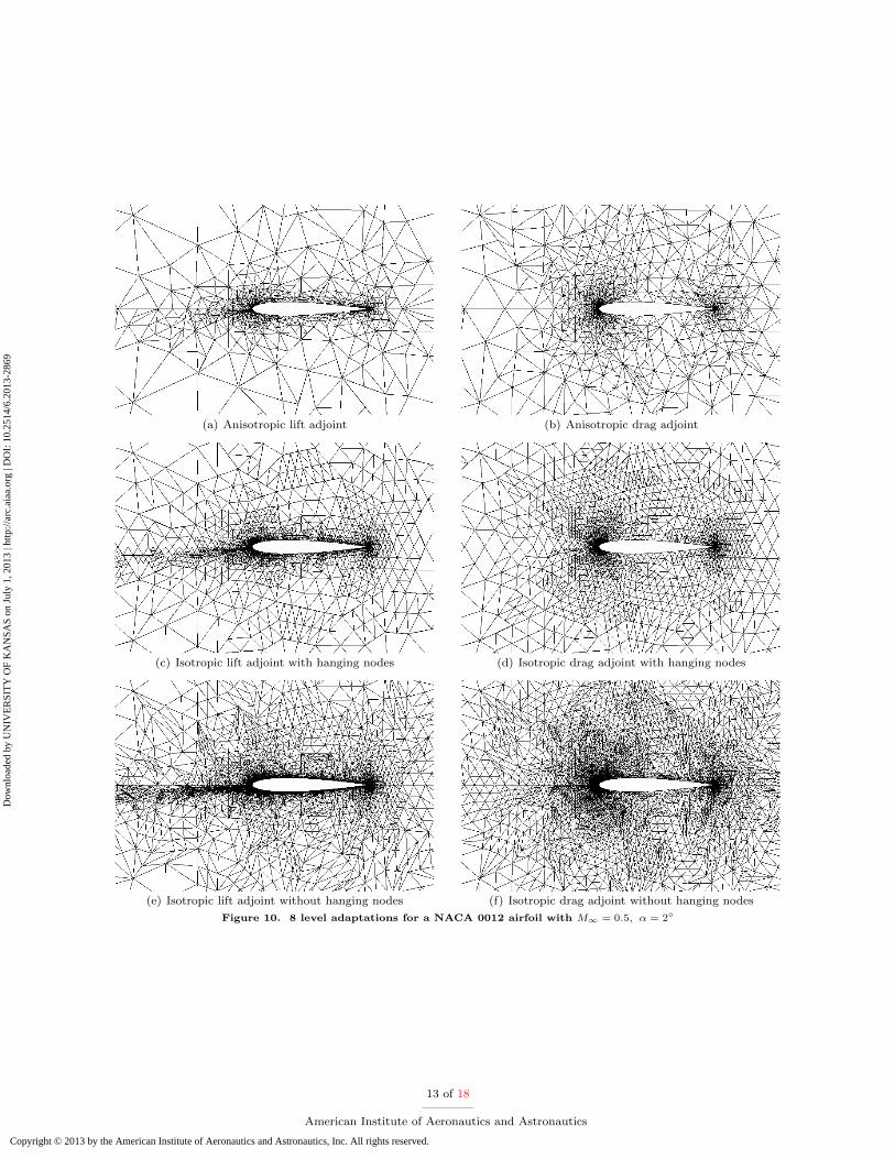
The first test case involves subsonic flow over a NACA 0012 airfoil with a free-stream Mach number ofM∞ = 0.5 and the angle of attack, α = 2. The ’truth’ lift coefficient of 0.286472 and drag coefficient of2.3e−6 are chosen from the finest level of the h-adaptation result. In order to reduce the influence from thefar field, the outer boundary is located 2000 chords away. The initial mesh is shown in Figure 7. All ofthe simulations undergo 12 levels of isotropic and anisotropic h-adaptations. For all of cases, the solutionpolynomial is p = 2 and refinement fraction f=0.1 is used. The drag coefficient and lift coefficient areconsidered as the output of interest. The final h-adapted meshes of each strategy are shown in Figure 10.For both of the anisotropic and isotropic adaptations, the regions near the trailing edge and the leading edgeare adapted consistently.

Figure 8 shows the convergence of the base and corrected lift and drag coefficients for all of the adaptationstrategies. When corrected by the output-based error estimates, the outputs converge much faster than thebase outputs. Figure 9 compares the lift coefficient error and drag coefficient error. It is clearly to see that,for test cases with the lift and drag adjoint as the output, the anisotropic h-adaptive methods could producemore efficient error reductions in term of the DOFs. Compare with the result of the isotropic adaptation with

11 of 18


Dow

nloa

ded

by U

NIV

ER

SIT

Y O

F K

AN

SAS

on J

uly

1, 2

013

| http

://ar

c.ai

aa.o

rg |

DO

I: 1

0.25

14/6

.201

3-28

69


Figure 7. The initial mesh for a NACA 0012 airfoil at M0 = 0.5, α = 2

DOFs

Cl

50000 1000001500002000000.286

0.2862

0.2864

0.2866

0.2868

0.287

Uniform refinement

Lift adj (iso, hanging)

Lift adj( iso, no hanging)

Lift adj(aniso, no hanging)

Lift adj (iso, hanging)corrLift adj(aniso, no hanging)corr

(a) CL

DOFs

Cd

50000 100000150000

0.0E+00

2.0E04

4.0E04

6.0E04

8.0E04

1.0E03

1.2E03 Uniform refinement

Drag adj(iso, hanging)

Drag adj(iso, no hanging)

Drag adj (aniso, no hanging)

Drag adj(iso, hanging)corr

Drag adj (aniso, no hanging)corr

(b) CD

Figure 8. The corrected outputs of the h-adaptations for a NACA 0012 airfoil at M0 = 0.5, α = 2

sqrt_dof

Cl

200 400 600 800

106

105

104

103

Uniform refinement

Lift adj (iso, hanging)

Lift adj( iso, no hanging)

Lift adj(aniso, no hanging)

(a) CL errorsqrt_dof

Cd

100 200 300 400 50

107

106

105

104

103

102

101

Uniform refinement

Drag adj(iso, hanging)

Drag adj(iso, no hanging

Drag adj (aniso, no hang

(b) CD errorFigure 9. The output error of the h-adaptations for a NACA 0012 airfoil at M0 = 0.5, α = 2

12 of 18


Dow

nloa

ded

by U

NIV

ER

SIT

Y O

F K

AN

SAS

on J

uly

1, 2

013

| http

://ar

c.ai

aa.o

rg |

DO

I: 1

0.25

14/6

.201

3-28

69


(a) Anisotropic lift adjoint (b) Anisotropic drag adjoint

(c) Isotropic lift adjoint with hanging nodes (d) Isotropic drag adjoint with hanging nodes

(e) Isotropic lift adjoint without hanging nodes (f) Isotropic drag adjoint without hanging nodes

Figure 10. 8 level adaptations for a NACA 0012 airfoil with M∞ = 0.5, α = 2

13 of 18


Dow

nloa

ded

by U

NIV

ER

SIT

Y O

F K

AN

SAS

on J

uly

1, 2

013

| http

://ar

c.ai

aa.o

rg |

DO

I: 1

0.25

14/6

.201

3-28

69


hanging nodes, the adaptation without hanging nodes waste some DOFs to refine their neighbors, which isnot necessarily required in term of minimizing functional error. Since there is a geometry singularity pointat the trailing edge of the airfoil and the initial mesh has relatively coarse elements near the trailing edge,the uniform mesh refinements can not achieve their expected order of accuracy. The current results showthat the h-adaptations successively refine the mesh around the trailing edge; therefore it could reduce theeffect of this geometry singularity and reveal the potential accuracy from the high order CPR method.

(a) Mach number contours with the lift adjoint (b) Mesh with the lift adjoint

Figure 11. Anisotropic h-adaptation for a NACA 0012 airfoil at M0 = 0.8, α = 1.25

V.B. Transonic Flow over a NACA 0012 Airfoil

The last test case is a NACA 0012 airfoil in inviscid transonic flow with an inflow Mach number M∞ = 0.8and the angle of attack, α = 1.25. Again, this test is the problem C1.3(b) of the 1st international workshopon high-order methods. The structure of the solution to this transonic problem includes shockwaves on theupper and lower surfaces of the airfoil.

All of the calculations start with an uniform solution order of p=2 and consistently refined using previouslydescribed adaptation procedure. The jump indicator

φk =1

|∂Ωk|

∫∂Ωk

|JqK · ~nq

|ds (52)

introduced in Ref. [63] is used to examine the smoothness of the primal solution and determine which cellshould be limited. Here, the pressure is used as the jump indicator variable q throughout this paper. Thesurface average operator · and the surface jump operator J·K are defined as

q =1

2(q+ + q−) (53)

JqK = ~n(q+ − q−),

where (·)+ and (·)− notations refer to the elements on each side of the edge. The criterion of the smoothnessφk >

1K , h− refinement

φk <1K , p− enrichment

, (54)

where K = 25 suggested in Ref. [64] and Ref. [65] is used. Once a cell with large jumps is marked, the orderof its solution polynomial is reduced to p=0. This approach can be treated as a spacial limiter; thereforethere is no need to use artificial viscosity to stabilize the solution in the presence of shocks. So we don’tneed to worry about any pollution to the adjoint solution by the artificial viscosities. However, it do causesome convergence problems for the primal solver.

The final mesh after 5 adaptation iterations is shown in Figure 11. The result shows that the shockwavesnear the upper and lower surfaces are correctly identified using the current adjoint-based error estimation

14 of 18


Dow

nloa

ded

by U

NIV

ER

SIT

Y O

F K

AN

SAS

on J

uly

1, 2

013

| http

://ar

c.ai

aa.o

rg |

DO

I: 1

0.25

14/6

.201

3-28

69


without any feature based smoothness indicators. Mach number with the lift output are plotted in Figure11(b).

VI. Conclusions

In this paper, we apply an anisotropic h-adaptation method on simplex meshes to minimize the functionalerror. An adjoint-based error estimation with a local refinement sampling process is utilized to drive theanisotropic mesh adaptation without making any assumption about the solution features. Several well-knowntwo-dimensional inviscid flow cases are utilized to compare the effectiveness of anisotropic and isotropicadjoint-based h-adaptations. The refinement driven by the adjoint-based error indicator can directly targetthe error source to the engineering output. Results show some savings of degrees of freedom for the anisotropicadaptations when compared with the isotropic refinements. For the simplex meshes, to fully obtain theadvantage of the DOF reductions inherited in the anisotropic meshes, grid re-generations may be required.We will further test the performance of the anisotropic h-adaptation of simplex meshes for viscous flow.

Acknowledgments

The authors gratefully acknowledge support by NASA under grant NNX12AK04A and AFOSR under grantFA95501210286.

References

1 Lhner, R., Morgan, K., Peraire, J., and Vahdati, M., “Finite element flux-corrected transport (FEMFCT)for the euler and NavierStokes equations,” International Journal for Numerical Methods in Fluids, Vol. 7,No. 10, 1987, pp. 1093–1109.

2 Castro-Daz, M. J., Hecht, F., Mohammadi, B., and Pironneau, O., “Anisotropic unstructured meshadaption for flow simulations,” International Journal for Numerical Methods in Fluids, Vol. 25, No. 4,1997, pp. 475–491.

3 Dompierre, J., Vallet, M., Bourgault, Y., Fortin, M., and Habashi, W., “Anisotropic mesh adaptation: to-wards user-independent, mesh-independent and solver-independent CFD. Part III. Unstructured meshes,”International journal for numerical methods in fluids, Vol. 39, No. 8, 2002, pp. 675–702.

4 Hartmann, R. and Houston, P., “Adaptive Discontinuous Galerkin Finite Element Methods for the Com-pressible Euler Equations,” Journal of Computational Physics, Vol. 183, No. 2, 2002, pp. 508 – 532.

5 Venditti, D. and Darmofal, D., “Anisotropic grid adaptation for functional outputs: application to two-dimensional viscous flows,” Journal of Computational Physics, Vol. 187, No. 1, 2003, pp. 22–46.

6 Venditti, D. A. and Darmofal, D. L., “Anisotropic grid adaptation for functional outputs: application totwo-dimensional viscous flows,” J. Comput. Phys., Vol. 187, No. 1, May 2003, pp. 22–46.

7 Fidkowski, K. and Darmofal, D., “A triangular cut-cell adaptive method for high-order discretizationsof the compressible Navier-Stokes equations,” Journal of Computational Physics, Vol. 225, No. 2, 2007,pp. 1653–1672.

8 Wang, L. and Mavriplis, D., “Adjoint-based hp adaptive discontinuous Galerkin methods for the 2Dcompressible Euler equations,” Journal of Computational Physics, Vol. 228, No. 20, 2009, pp. 7643–7661.

9 Fidkowski, K., “Review of Output-Based Error Estimation and Mesh Adaptation in Computational FluidDynamics,” AIAA Journal , Vol. 49, No. 4, 2011, pp. 673–694.

10 Baumann, C. and Oden, J., “A discontinuous hp finite element method for the Euler and Navier–Stokesequations,” International Journal for Numerical Methods in Fluids, Vol. 31, No. 1, 1999, pp. 79–95.

11 Devloo, P., Tinsley Oden, J., and Pattani, P., “An hp adaptive finite element method for the numericalsimulation of compressible flow,” Computer methods in applied mechanics and engineering , Vol. 70, No. 2,1988, pp. 203–235.

15 of 18


Dow

nloa

ded

by U

NIV

ER

SIT

Y O

F K

AN

SAS

on J

uly

1, 2

013

| http

://ar

c.ai

aa.o

rg |

DO

I: 1

0.25

14/6

.201

3-28

69


12 Bassi, F. and Rebay, S., “High-order accurate discontinuous finite element solution of the 2D Eulerequations,” Journal of Computational Physics, Vol. 138, No. 2, 1997, pp. 251–285.

13 Cockburn, B. and Shu, C., “The Runge–Kutta discontinuous Galerkin method for conservation laws V:multidimensional systems,” Journal of Computational Physics, Vol. 141, No. 2, 1998, pp. 199–224.

14 Liu, Y., Vinokur, M., and Wang, Z., “Spectral (finite) volume method for conservation laws on unstruc-tured grids V: extension to three-dimensional systems,” Journal of Computational Physics, Vol. 212,No. 2, 2006, pp. 454–472.

15 Wang, Z., “Spectral (Finite) Volume Method for Conservation Laws on Unstructured Grids. Basic For-mulation:: Basic Formulation,” Journal of Computational Physics, Vol. 178, No. 1, 2002, pp. 210–251.

16 Liu, Y., Vinokur, M., and Wang, Z., “Discontinuous spectral difference method for conservation laws onunstructured grids,” Computational Fluid Dynamics 2004 , 2006, pp. 449–454.

17 Huynh, H. T., “A flux reconstruction approach to high-order schemes including discontinuous Galerkinmethods,” Aiaa paper 2007–4079, 2007.

18 Wang, Z. J. and Gao, H., “A unifying lifting collocation penalty formulation including the discontin-uous Galerkin, spectral volume/difference methods for conservation laws on mixed grids,” Journal ofComputational Physics, Vol. 228, 2009, pp. 8161–8186.

19 Haga, T., Gao, H., and Wang, Z. J., “A High-Order Unifying Discontinuous Formulation for the Navier-Stokes Equations on 3D Mixed Grids,” Mathematical Modelling of Natural Phenomena, Vol. 6, 2011,pp. 28–56.

20 Gao, H. and Wang, Z. J., “A conservative correction procedure via reconstruction formulation with theChain-Rule divergence evaluation,” Journal of Computational Physics, Vol. 232, Jan. 2013, pp. 7–13.

21 Castonguay, P., Vincent, P. E., and Jameson, A., “A New Class of High-Order Energy Stable FluxReconstruction Schemes for Triangular Elements,” J. Sci. Comput., Vol. 51, No. 1, April 2012, pp. 224–256.

22 Jameson, A., Vincent, P. E., and Castonguay, P., “On the Non-linear Stability of Flux ReconstructionSchemes,” J. Sci. Comput., Vol. 50, No. 2, Feb. 2012, pp. 434–445.

23 Cagnone, J., Vermeire, B., and Nadarajah, S., “A p-adaptive LCP formulation for the compressibleNavierStokes equations,” Journal of Computational Physics, Vol. 233, No. 0, 2013, pp. 324 – 338.

24 Berger, M. and Colella, P., “Local adaptive mesh refinement for shock hydrodynamics,” Journal ofcomputational Physics, Vol. 82, No. 1, 1989, pp. 64–84.

25 Warren, G., Anderson, W., Thomas, J., and Krist, S., “Grid convergence for adaptive methods,” 10thAIAA Computational Fluid Dynamics Conference, 1991.

26 Barth, T., “Numerical methods for gasdynamic systems on unstructured meshes,” An Introduction toRecent Developments in Theory and Numerics for Conservation Laws, Vol. 5, 1998, pp. 195–285.

27 Harris, R. and Wang, Z., “High-order adaptive quadrature-free spectral volume method on unstructuredgrids,” Computers & Fluids, Vol. 38, No. 10, 2009, pp. 2006–2025.

28 Ainsworth, M. and Oden, J., “A unified approach to a posteriori error estimation using element residualmethods,” Numerische Mathematik , Vol. 65, No. 1, 1993, pp. 23–50.

29 Baker, T. J., “Mesh adaptation strategies for problems in fluid dynamics,” Finite Elements in Analysisand Design, Vol. 25, No. 34, 1997, pp. 243 – 273, ¡ce:title¿Adaptive Meshing, Part 2¡/ce:title¿.

30 Johnson, C., “Adaptive finite element methods for conservation laws,” Advanced numerical approximationof nonlinear hyperbolic equations, 1998, pp. 269–323.

31 Shih, T. and Qin, Y., “A Posteriori Method for Estimating and Correcting Grid-Induced Errors in CFDSolutions–Part 1: Theory and Method,” AIAA Paper , Vol. 100, 2007.

16 of 18


Dow

nloa

ded

by U

NIV

ER

SIT

Y O

F K

AN

SAS

on J

uly

1, 2

013

| http

://ar

c.ai

aa.o

rg |

DO

I: 1

0.25

14/6

.201

3-28

69


32 Gao, H. and Wang, Z., “A residual-based procedure for hp-adaptation on 2d hybrid meshes,” AIAAPaper , Vol. 492, 2011, pp. 2011.

33 Cagnone, J. and Nadarajah, S., “A stable interface element scheme for the p-adaptive lifting collocationpenalty formulation,” Journal of Computational Physics, Vol. 231, No. 4, 2012, pp. 1615 – 1634.

34 Giles, M. and Pierce, N., “Adjoint equations in CFD: duality, boundary conditions and solution be-haviour,” AIAA paper , Vol. 97, 1997, pp. 1850.

35 Venditti, D. A. and Darmofal, D. L., “Adjoint error estimation and grid adaptation for functional outputs:application to quasi-one-dimensional flow,” J. Comput. Phys., Vol. 164, No. 1, Oct. 2000, pp. 204–227.

36 Becker, R. and Rannacher, R., “An optimal control approach to a posteriori error estimation in finiteelement methods,” Acta Numerica, Vol. 10, 2001, pp. 1–102.

37 Giles, M. and Pierce, N., “Adjoint error correction for integral outputs,” 2001.

38 Park, M., “Adjoint-based, three-dimensional error prediction and grid adaptation,” AIAA paper , Citeseer,2002.

39 Leicht, T. and Hartmann, R., “Error estimation and anisotropic mesh refinement for 3d laminar aerody-namic flow simulations,” J. Comput. Phys., Vol. 229, No. 19, Sept. 2010, pp. 7344–7360.

40 Li, Y., Allaneau, Y., and Jameson, A., “Continuous Adjoint Approach for Adaptive Mesh Renement,”AIAA Paper , Vol. 3982, 2010, pp. 2011.

41 Yano, M. and Darmofal, D. L., “An optimization-based framework for anisotropic simplex mesh adapta-tion,” J. Comput. Phys., Vol. 231, No. 22, Sept. 2012, pp. 7626–7649.

42 Ceze, M. and Fidkowski, K. J., “Anisotropic hp-Adaptation Framework for Functional Prediction,” AIAAJournal , Vol. 51, No. 2, 2012, pp. 492–509.

43 Zhang, X., Vallet, M.-G., Dompierre, J., Labbe, P., Pelletier, D., and Trepanier, J.-Y., “Mesh adaptationusing dierent error indicators for the Euler equations,” Aiaa paper 2001–2549, 2001.

44 Fidkowski, K. and Roe, P., “Entropy-based Mesh Refinement, I: The Entropy Adjoint Approach,” 2009.

45 Fidkowski, K. and Roe, P., “An entropy adjoint approach to mesh refinement,” SIAM Journal on ScientificComputing , Vol. 32, No. 3, 2010, pp. 1261–1287.

46 Peraire, J., Vahdati, M., Morgan, K., and Zienkiewicz, O., “Adaptive remeshing for compressible flowcomputations,” Journal of Computational Physics, Vol. 72, No. 2, 1987, pp. 449 – 466.

47 Loseille, A., Dervieux, A., and Alauzet, F., “Fully anisotropic goal-oriented mesh adaptation for 3Dsteady Euler equations,” J. Comput. Phys., Vol. 229, No. 8, April 2010, pp. 2866–2897.

48 Formaggia, L., Micheletti, S., and Perotto, S., “Anisotropic mesh adaptation in computational fluiddynamics: Application to the advectiondiffusionreaction and the Stokes problems,” Applied NumericalMathematics, Vol. 51, No. 4, 2004, pp. 511 – 533, ¡ce:title¿Applied Scientific Computing: Advances inGrid Generatuion, Approximation and Numerical Modeling¡/ce:title¿.

49 Leicht, T. and Hartmann, R., “Anisotropic mesh refinement for discontinuous Galerkin methods intwo-dimensional aerodynamic flow simulations,” International Journal for Numerical Methods in Flu-ids, Vol. 56, No. 11, 2008, pp. 2111–2138.

50 Georgoulis, E. H., Hall, E., and Houston, P., “Discontinuous Galerkin methods on hp-anisotropic meshesII: a posteriori error analysis and adaptivity,” Appl. Numer. Math., Vol. 59, No. 9, Sept. 2009, pp. 2179–2194.

51 Li, Y., Premasuthan, S., and Jameson, A., “Comparison of h-and p-Adaptations for Spectral DifferenceMethods,” AIAA Paper , Vol. 4435, 2010, pp. 2010.

17 of 18


Dow

nloa

ded

by U

NIV

ER

SIT

Y O

F K

AN

SAS

on J

uly

1, 2

013

| http

://ar

c.ai

aa.o

rg |

DO

I: 1

0.25

14/6

.201

3-28

69


52 Hartmann, R., “Adjoint consistency analysis of Discontinuous Galerkin discretizations,” SIAM J. Numer.Anal., Vol. 45, No. 6, 2007, pp. 2671–2696.

53 K. Duraisamy, J. J. Alonso, F. P. and Chandrashekar, P., “Error Estimation for High Speed Flows UsingContinuous and Discrete Adjoints,” Aiaa paper 2010–128, 2010.

54 Huynh, H. T., “A Reconstruction Approach to High-Order Schemes Including Discontinuous Galerkin forDiffusion,” Aiaa paper 2009-403, 2009.

55 T. Haga, H. G. and Wang, Z. J., “A High-Order Unifying Discontinuous Formulation for the Navier-StokesEquations on 3D Mixed Grids,” Math. Model. Nat. Phenom., Vol. 6, No. 03, 2011, pp. 28–56.

56 Wang, Z. J., Adaptive High-Order Methods in Computational Fluid Dynamics, World Scientific Publish-ing, May 2011.

57 Godunov, S. K., “A finite-difference method for the numerical computation of discontinuous solutions ofthe equations of fluid dynamics,” Mat. Sb., Vol. 47, 1959, pp. 271.

58 Leer, B. V., “Towards the ultimate conservative difference scheme V. a second order sequel to Godunovsmethod,” J. Comput. Phys., Vol. 32, 1979, pp. 101–136.

59 Liou, M.-S., “A sequel to AUSM, Part II: AUSM+-up for all speeds,” J. Comput. Phys., Vol. 214, 2006,pp. 137–170.

60 Roe, P. L., “Approximate Riemann solvers, parameter vectors, and difference schemes,” J. Comput. Phys.,Vol. 43, 1981, pp. 357–372.

61 Rusanov, V. V., “Calculation of interaction of non-steady shock waves with obstacles,” J. Comput. Phys.,Vol. 1, 1961, pp. 261–279.

62 Lu, J. C.-C., An a posteriori Error Control Framework for Adaptive Precision Optimization using Dis-continuous Galerkin Finite Element Method , Ph.D. thesis, Massachusetts Institute of Technology, 2005.

63 Krivodonova, L., Xin, J., Remacle, J.-F., Chevaugeon, N., and Flaherty, J., “Shock detection and limitingwith discontinuous Galerkin methods for hyperbolic conservation laws,” Applied Numerical Mathematics,Vol. 48, No. 34, 2004, pp. 323 – 338, ¡ce:title¿Workshop on Innovative Time Integrators for PDEs¡/ce:title¿.

64 Burgess, N., An Adaptive Discontinuous Galerkin Solver for Aerodynamic Flows, Ph.D. thesis, Universityof Wyoming, 2011.

65 Wang, L. and Mavriplis, D. J., “Adjoint-based h-p adaptive discontinuous Galerkin methods for the 2Dcompressible Euler equations,” J. Comput. Phys., Vol. 228, No. 20, Nov. 2009, pp. 7643–7661.

18 of 18


Dow

nloa

ded

by U

NIV

ER

SIT

Y O

F K

AN

SAS

on J

uly

1, 2

013

| http

://ar

c.ai

aa.o

rg |

DO

I: 1

0.25

14/6

.201

3-28

69


Download - Adjoint Based Anisotropic Mesh Adaptation for the CPR …dept.ku.edu/~cfdku/papers/AIAA-2013-2869.pdf · Adjoint Based Anisotropic Mesh Adaptation for the ... 10.2514/6.2013-2869

Top Related