Download - Adaptive Filter Theory

DESIGN AND IMPLEMENTATION OF A FIXED POINT DIGITAL
ACTIVE NOISE CONTROLLER HEADPHONE
A THESIS SUBMITTED TO
THE GRADUATE SCHOOL OF NATURAL AND APPLIED SCIENCES
OF
MIDDLE EAST TECHNICAL UNIVERSITY
BY
FATİH ERKAN
IN PARTIAL FULFILLMENT OF THE REQUIREMENTS
FOR
THE DEGREE OF MASTER OF SCIENCE
IN
ELECTRICAL AND ELECTRONICS ENGINEERING
JULY 2009
Approval of the thesis:
DESIGN AND IMPLEMENTATION OF A FIXED POINT DIGITAL
ACTIVE
NOISE CONTROLLER HEADPHONE
submitted by FATİH ERKAN in partial fulfillment of the requirements for the
degree of Master of Science in Electrical and Electronics Engineering
Department, Middle East Technical University by,
Prof. Dr. Canan Özgen
Dean, Graduate School of Natural and Applied Sciences __________
Prof. Dr. İsmet Erkmen
Head of Department, Electrical and Electronics Engineering ______
Assoc. Prof. Dr. Tolga Çiloğlu
Supervisor, Electrical and Electronics Engineering Dept., METU ______
Examining Committee Members
Prof. Dr. Mübeccel Demirekler
Electrical and Electronics Engineering Dept., METU __________
Assoc. Prof. Dr. Tolga Çiloğlu
Electrical and Electronics Engineering Dept., METU __________
Assist. Prof. Çağatay Candan
Electrical and Electronics Engineering Dept., METU __________
Assist. Prof. Emre Tuna
Electrical and Electronics Engineering Dept., METU __________
Dr. Bekir Ahmet Doğrusöz
ASELSAN __________
Date: 29.07.2009

iii
I hereby declare that all information in this document has been obtained
and presented in accordance with academic rules and ethical conduct. I also
declare that, as required by these rules and conduct, I have fully cited and
referenced all material and results that are not original to this work.
Name, Last name : Fatih Erkan
Signature :

iv
ABSTRACT
DESIGN AND IMPLEMENTATION OF A FIXED POINT DIGITAL
ACTIVE NOISE CONTROLLER HEADPHONE
Erkan, Fatih
M. Sc., Department of Electrical and Electronics Engineering
Supervisor: Assoc. Prof. Dr. Tolga Çiloğlu
July 2009, 106 pages
In this thesis, the design and implementation of a Portable Feedback Active
Noise Controller Headphone System, which is based on Texas Instruments
TMS320VC5416PGE120 Fixed Point DSP, is described. Problems resulted from fixed-
point implementation of LMS algorithm and delays existing in digital ANC
implementation are determined. Effective solutions to overcome the aforementioned
problems are proposed based on the literature survey. Design of the DSP based control
card is explained and crucial points about analog-digital-mixed board design for noise
sensitive applications are explained. Filtered input LMS algorithm, filtered input
normalized LMS algorithm and filtered input sign-sign LMS algorithm are implemented
as adaptation algorithms. The advantages and disadvantages of using modified LMS
algorithms are indicated. The selection of the parameters of these algorithms is based on
theoretical results and experiments. The real time performances of different adaptation
algorithms are compared with each other as well as with a commercial analog ANC
headphone under different types of artificial and natural noise signals. Moreover,
practical conditions such as put on - put off case and dynamic range overflow case are
handled with additional software implementations. It is shown that adaptive ANC

v
systems improve the noise reduction significantly when the noise is within a narrow
frequency range and this reduction can be applied to a wider frequency range. It is also
shown that the problems of digitally implemented adaptive filters which are based on
tracking capability, stability, dynamic range and portability can be fixed to challenge
with the analog commercial ANC systems.
Keywords: Filtered Input LMS, Feedback Active Noise Control, Fixed Point
Implementation of Active Noise Control, Digital Residual Error, Slowdown
Phenomenon in Fixed Point LMS

vi
ÖZ
SABİT NOKTALI SAYISAL AKTİF GÜRÜLTÜ ENGELLEYİCİ
KULAKLIK TASARIMI VE UYGULAMASI
Yüksek Lisans, Elektrik ve Elektronik Mühendisliği Bölümü
Tez yöneticisi: Doç. Dr. Tolga Çiloğlu
Temmuz 2009, 106 sayfa
Bu tezde, Sabit Noktalı TMS320VC5416 Sayısal Sinyal İşleyici Tabanlı
Taşınabilir Aktif Gürültü Engelleyici Kulaklık tasarım ve uygulaması anlatılmıştır.
Sabit-nokta uygulamasından ve sayısal aktif gürültü uygulamasındaki gecikmelerden
kaynaklanan problemler belirtilmiştir. Belirtilen problemler için literatür araştırması
sonucu etkili çözümler bulunmuştur. Sayısal Sinyal İşleyici tabanlı kart tasarımı
irdelenmiş ve gürültü hassasiyeti yüksek analog-sayısal-karışık kart tasarımının kritik
noktaları belirtilmiştir. Adaptasyon algoritmaları olarak, filtrelenmiş giriş sinyali
kullanımlı LMS, normalize LMS ve sign-sign LMS algoritmaları uygulanmıştır.
Kullanılan algoritmaların avantaj ve dezavantajları belirtilmiştir. Bu algoritmaların
parametrelerinin seçimi hususunda teorik çıkarımlar ve deneyler kullanılmıştır. Farklı
adaptasyon algortimalarının gerçek zamanlı performansları birbirleriyle ve halen
piyasada ticari ürün olarak kullanım alanı bulan analog aktif gürültü engelleyici bir
kulaklık ile suni ve doğal gürültüler altında kıyaslanmıştır. Bunun ötesinde, kullanım
sırasında problem oluşturabilecek, kulaklığın takılıp çıkarılması veya dinamik aralığı
aşan gürültü seviyelerine maruz kalınması gibi durumların bertaraf edilmesi için
yazılımsal düzeltmeler eklenmiştir. Bu çalışmada gürültü sinyallerinin dar bantta olması
durumunda sayısal sistemlerin gürültü azaltımını fark edilir seviyede arttırdığı ve bu
artışın daha geniş bantlara da taşınabileceği gösterilmiştir. Ayrıca, sayısal sistemlerin
problem yaşadıkları takip edebilme yeteneği, stabil çalışma, dinamik aralık ve

vii
taşınabilirlik konularında geliştirilebilecekleri ve analog aktif gürültü engelleyici
kulaklıklarla rekabet edebilecekleri gösterilmiştir.
Anahtar Kelimeler: Filtrelenmiş Giriş Sinyali Kullanımlı Geri Besleme, Aktif Gürültü
Kontrol Sistemi, Aktif Gürültü Kontrolünün Sabit-Nokta Uygulaması, Sayısal Kalan
Hata, Sabit-Nokta LMS uygulamasında Yavaşlama Fenomeni

viii
To My Wife

ix
ACKNOWLEDGMENTS
I would like to thank to my supervisor Assoc. Prof. Dr. Tolga Çiloğlu for his
guidance and encouragement.
I also would like to thank to Tübitak for their financial support to this study.
x
TABLE OF CONTENTS
ABSTRACT ...................................................................................................................... iv
ÖZ ..................................................................................................................................... vi
ACKNOWLEDGMENTS ................................................................................................ ix
TABLE OF CONTENTS ................................................................................................... x
LIST OF TABLES ......................................................................................................... xiii
LIST OF FIGURES ........................................................................................................ xiv
LIST OF ABBREVIATIONS ......................................................................................... xix
CHAPTERS
1. INTRODUCTION ......................................................................................................... 1
1.1 Scope of the Thesis ........................................................................................ 4
1.2 Outline of the Thesis ...................................................................................... 4
2. ADAPTIVE FILTER THEORY .................................................................................... 6
2.1 Wiener Filter Theory ...................................................................................... 6
2.2 Least Mean Square Algortihm ....................................................................... 9
2.3 Recursive Least Square Algorithm vs. Least Mean Square Algorithm ....... 10
2.4 Modified Least Mean Square Algorithms .................................................... 11
2.4.1 Normalized Least Mean Square Algorithm ......................................... 11
2.4.2 Sign-Sign Least Mean Square Algorithm ............................................ 11
3. ADAPTIVE ACTIVE NOISE CONTROL THEORY ................................................ 13
3.1 Feedforward Active Noise Control .............................................................. 13
3.2 Feedback Active Noise Control ................................................................... 14
3.3 Secondary Path Transfer Function in ANC Systems ................................... 16
3.4 Filtered Input LMS Algorithm ..................................................................... 17
3.5 Offline Secondary Path Modeling Procedure .............................................. 19
3.6 Single Channel Feedback Active Noise Control System ............................. 21
4. EFFECTS OF FINITE PRECISION ON ADAPTIVE FILTERS ............................... 24
4.1 The Quantization Error of MSE in Finite Precision Adaptive Filters .......... 25
xi
4.2 The Slowdown Phenomenon in Finite Precision Adaptation ...................... 26
4.3 Advantage of Power-of-Two Step Size Selection in Finite Precision ......... 28
5. ACTIVE NOISE CONTROL COMPUTER SIMULATIONS ................................... 29
5.1 Secondary Path Model Simulations ............................................................. 29
5.2 Noise Cancellation Simulations ................................................................... 31
6. DESIGN OF PORTABLE DIGITAL ANC HEADPHONE SYSTEM ...................... 35
6.1 Schematic Design ......................................................................................... 35
6.2 DSP Configuration ....................................................................................... 38
6.3 CODEC Configuration ................................................................................. 39
6.4 DSP Software for ANC Headphone System ................................................ 40
7. REAL TIME FEEDBACK ACTIVE NOISE CONTROL IMPLEMENTATION ..... 41
7.1 A Practical Approach about Delays in Fx-LMS in ANC Application ......... 41
7.2 The Software Architecture of Fx-LMS ANC............................................... 45
7.3 Fixed Point Limitations in LMS Active Noise Control Implementation ..... 48
7.4 The Discussion of Modified LMS Algorithms in Fixed Point ..................... 50
7.5 Software Implementation of Offline Secondary Path Modeling.................. 51
7.6 Additional Software Implementations ......................................................... 53
8. PERFORMANCE TESTS OF THE DIGITAL ANC HEADPHONE ........................ 55
8.1 Single Tone Experiments ............................................................................. 56
8.2 Multiple Tone Experiments ......................................................................... 59
8.3 Fan Noise Experiments ................................................................................ 64
8.4 Propeller Cabin Noise Experiments ............................................................. 69
8.5 Drill Noise Experiments ............................................................................... 73
8.6 Tracking Capability Experiments ................................................................ 78
8.7 Convergence Rate for Different LMS Algorithms....................................... 80
8.8 Digital Residual Error Experiment............................................................... 82
8.9 Drill Noise Experiment: Sub-band Filtering ................................................ 88
8.10 Discussion of the Test Results of Digital ANC Headphone System ........... 90
9. CONCLUSION ............................................................................................................ 92
9.1 Future Work ................................................................................................. 94
REFERENCES ................................................................................................................. 96

xii
APPENDICES
A. HARDWARE DESIGN OF DIGITAL ANC HEADPHONE SYSTEM ................... 99
B. TMS320VC5416 DSP CONFIGURATION ............................................................. 101
C. TLV320AIC20K CODEC CONFIGURATION ....................................................... 104

xiii
LIST OF TABLES
TABLES
Table 8.1 – The attenuation levels of single tones for digital and analog system............ 58
Table 8.2 – The attenuation levels of multi tone composed of 100 Hz(dominant), 200
Hz(small), 300 Hz(small), 400 Hz(smaller) and 500 Hz(smaller) ................................... 63
Table 8.3 – The attenuation levels of multi tone composed of 200 Hz(dominant), 600
Hz(small), 800 Hz(smaller) .............................................................................................. 63
Table 8.4 – The attenuation levels of multi tone composed of 100 Hz(dominant), 400
Hz(small) and 900 Hz(smaller) ........................................................................................ 64
Table 8.5 - The attenuation levels of fan noise ................................................................ 68
Table 8.6 - The attenuation levels of propeller cabin noise ............................................. 73
Table 8.7 - The attenuation levels of drill noise............................................................... 77
Table C.1 – TLV320AIC20K CODEC Write Register Form ........................................ 105
Table C.2 - TLV320AIC20K CODEC Register Content............................................... 106

xiv
LIST OF FIGURES
FIGURES
Figure 2.1 – Wiener Filter Block Diagram ........................................................................ 6
Figure 3.1 – Feedforward Active Noise Control System Configuration ......................... 13
Figure 3.2 – Feedforward Active Noise Control System Block Diagram ....................... 14
Figure 3.3 – Feedback Active Noise Control System Configuration .............................. 15
Figure 3.4 – Feedback Active Noise Control Block Diagram ......................................... 15
Figure 3.5 – Block Diagram of Transfer Functions between Input and Output of
Adaptive Feedback Controller ......................................................................................... 16
Figure 3.6 – Secondary Path Model Transfer Function of Feedback ANC system ......... 16
Figure 3.7 – Filtered Input LMS Algorithm Block Diagram ........................................... 17
Figure 3.8 – Block Diagram of Secondary Path Modeling in ANC Systems .................. 20
Figure 3.9 - Filtered Input LMS Algorithm Block Diagram ............................................ 22
Figure 3.10 - Filtered Input LMS Algorithm in Feedback System with Primary Signal
Estimation Block .............................................................................................................. 22
Figure 5.1 – An Accurate Secondary Path Model Estimation of Pure Delay in MATLAB
.......................................................................................................................................... 30
Figure 5.2 – An Improper Secondary Path Model Estimation of Pure Delay in MATLAB
due to Step Size Selection Mistake .................................................................................. 30
Figure 5.3 – An Improper Secondary Path Model Estimation of Pure Delay in MATLAB
due to Insufficient Iteration .............................................................................................. 31
Figure 5.4 – Fourier Transform of Primary Noise Signal in ANC Simulation in
MATLAB ......................................................................................................................... 32
Figure 5.5 – The Decreasing Characteristic of Error Signal by a Proper Adaptation
Process due to Suitable Step Size Selection in MATLAB ............................................... 32
Figure 5.6 – Adaptation Filter Coefficients of a Converged Simulation in MATLAB ... 33
Figure 5.7 – Faster Convergence due to a Larger Step Size within the Boundary of
Convergence in MATLAB ............................................................................................... 33

xv
Figure 5.8 – Convergence Rate with The Accurate Retrieval of Primary Noise in
MATLAB ......................................................................................................................... 34
Figure 5.9 – Slower Convergence Rate Because of The Inaccurate Retrieval of Primary
Noise in MATLAB .......................................................................................................... 34
Figure 6.1 – The Digital ANC System Hardware ............................................................ 36
Figure 6.2 – Generalized Block Diagram of the DSP Code for Fx-LMS Adaptive ANC
Headphone System ........................................................................................................... 40
Figure 7.1 - The Sampling of Error Signal in Real Time Implementation of ANC
Headphone System ........................................................................................................... 42
Figure 7.2 - Filtered Input LMS Algorithm in Feedback System .................................... 42
Figure 7.2 - Overall Block Diagram of Software Implementation for Fx-LMS in
Feedback ANC Headphone System ................................................................................. 47
Figure 7.3 – Block Diagram of Software Realization of Offline Secondary Path
Modeling in ANC Headphone System ............................................................................. 52
Figure 7.4 – The impulse response of Secondary Path Model of Active ANC Headphone
System .............................................................................................................................. 53
Figure 8.1 – Single 200 Hz Tone in NLMS Experiment “with ANC” and “without ANC”
.......................................................................................................................................... 56
Figure 8.2 – Fourier Transform of Single 200 Hz Tone in NLMS Experiment “without
ANC” ............................................................................................................................... 57
Figure 8.3 – Fourier Transform of Single 200 Hz Tone in NLMS Experiment “with
ANC” ............................................................................................................................... 57
Figure 8.4 - Tone of 100 Hz, 200Hz, 300Hz, 400Hz and 500 Hz Composition in NLMS
Experiment “with ANC” and “without ANC” ................................................................. 59
Figure 8.5 – Fourier Transform of 100 Hz, 200Hz, 300Hz, 400Hz and 500 Hz
Composition in NLMS Experiment “without ANC” ....................................................... 60
Figure 8.6 – Fourier Transform of 100 Hz, 200Hz, 300Hz, 400Hz and 500 Hz
Composition in NLMS Experiment “with ANC” ............................................................ 60
Figure 8.7 – Fourier Transform of Multi Tone Signal in LMS Digital Headphone
Experiment “with ANC” and “without ANC” ................................................................. 61

xvi
Figure 8.8 – Fourier Transform of Multi Tone Signal in LMS Digital Headphone
Experiment “with ANC” and “without ANC” ................................................................. 61
Figure 8.9 – Fourier Transform of Multi Tone Signal in Sign-Sign LMS Digital
Headphone Experiment “with ANC” and “without ANC” .............................................. 62
Figure 8.10 – Fourier Transform of Multi Tone Signal in Analog ANC Headphone
Experiment “with ANC” and “without ANC” ................................................................. 62
Figure 8.11 - Fan Noise in NLMS Experiment “with ANC” and “without ANC” .......... 65
Figure 8.12 – Fourier Transform of Fan Noise in NLMS Experiment “without ANC” .. 65
Figure 8.13 – Fourier Transform of Fan Noise in NLMS Experiment “with ANC” ....... 66
Figure 8.14 - Fourier Transform of Fan Noise in NLMS Experiment “with ANC” and
“without ANC” ................................................................................................................ 66
Figure 8.15 - Fourier Transform of Fan Noise in LMS Experiment “with ANC” and
“without ANC” ................................................................................................................ 67
Figure 8.16 - Fourier Transform of Fan Noise in Sign-Sign LMS Experiment “with
ANC” and “without ANC”............................................................................................... 67
Figure 8.17 - Fourier Transform of Fan Noise in Analog ANC Headphone Experiment
“with ANC” and “without ANC” ..................................................................................... 68
Figure 8.18 - Propeller Cabin Noise in LMS Experiment “with ANC” and “without
ANC” ............................................................................................................................... 69
Figure 8.19 – Fourier Transform of Propeller Cabin Noise in LMS Experiment “without
ANC” ............................................................................................................................... 70
Figure 8.20 – Fourier Transform of Propeller Cabin Noise in LMS Experiment “with
ANC” ............................................................................................................................... 70
Figure 8.21 - Fourier Transform of Propeller Cabin Noise in NLMS Experiment “with
ANC” and “without ANC”............................................................................................... 71
Figure 8.22 - Fourier Transform of Propeller Cabin Noise in LMS Experiment “with
ANC” and “without ANC”............................................................................................... 71
Figure 8.23 - Fourier Transform of Propeller Cabin Noise in Sign-Sign LMS Experiment
“with ANC” and “without ANC” ..................................................................................... 72
Figure 8.24 - Fourier Transform of Propeller Cabin Noise in ......................................... 72
Analog ANC Headphone Experiment “with ANC” and “without ANC”........................ 72
xvii
Figure 8.25 - Drill Noise in Sign-Sign LMS Experiment “with ANC” and “without
ANC” ............................................................................................................................... 74
Figure 8.26 – Fourier Transform of Drill Noise in Sign-Sign LMS Experiment “without
ANC” ............................................................................................................................... 74
Figure 8.27 - Fourier Transform of Drill Noise in Sign-Sign LMS Experiment “with
ANC” ............................................................................................................................... 75
Figure 8.28 - Fourier Transform of Drill Noise in NLMS Experiment “with ANC” and
“without ANC” ................................................................................................................ 75
Figure 8.29 - Fourier Transform of Drill Noise in LMS Experiment “with ANC” and
“without ANC” ................................................................................................................ 76
Figure 8.30 - Fourier Transform of Drill Noise in Sign-Sign LMS Experiment “with
ANC” and “without ANC”............................................................................................... 76
Figure 8.31 - Fourier Transform of Drill Noise in Analog ANC Headphone Experiment
“with ANC” and “without ANC” ..................................................................................... 77
Figure 8.32 – NLMS Tracking Performance with a Non-stationary Sinusoidal Signal .. 78
Figure 8.33 – LMS Tracking Performance with a Non-stationary Sinusoidal Signal ..... 78
Figure 8.34 – Sign-Sign LMS Tracking Performance with a Non-stationary Sinusoidal
Signal ............................................................................................................................... 79
Figure 8.35 – Analog ANC Headphone Performance with a Non-stationary Sinusoidal
Signal ............................................................................................................................... 79
Figure 8.36 – Convergence Rate of NLMS for Single Tone of 300 Hz .......................... 80
Figure 8.37 – Convergence Rate of LMS for Single Tone of 300 Hz ............................. 81
Figure 8.38 – Convergence Rate of Sign-Sign LMS for Single Tone of 300 Hz ............ 81
Figure 8.39 – Primary Noise for LMS Experiments for level-2 400 Hz signal ............... 82
Figure 8.40 – Residual Error for NLMS Experiment for level-2 400 Hz signal ............. 83
Figure 8.41 – Residual Error for LMS Experiment for level-2 400 Hz signal ................ 83
Figure 8.42 – Residual Error for Sign-Sign LMS Experiment for level-2 400 Hz signal84
Figure 8.43 – Primary Noise for LMS Experiments for level-1 400 Hz signal ............... 84
Figure 8.44 – Residual Error for NLMS Experiment for level-1 400 Hz signal ............. 85
Figure 8.45 – Residual Error for LMS Experiment for level-1 400 Hz signal ................ 85
Figure 8.46 – Residual Error for Sign-Sign LMS Experiment for level-1 400 Hz signal86

xviii
Figure 8.47 – Primary Noise for LMS Experiments for level-0 400 Hz signal ............... 86
Figure 8.48 – Residual Error for NLMS Experiment for level-0 400 Hz signal ............. 87
Figure 8.49 – Residual Error for LMS Experiment for level-0 400 Hz signal ................ 87
Figure 8.50 – Residual Error for Sign-Sign LMS Experiment for level-0 400 Hz signal88
Figure A.1 – Serial Port Connections between TLV320AIC20K and DSP .................... 99
Figure B.1 – Block Diagram of Multichannel Buffered Serial Port in TMS320VC5416
DSP ................................................................................................................................ 103
Figure C.1 – The Block Diagram of One Channel of TLV320AIC20K CODEC ......... 104
xix
LIST OF ABBREVIATIONS
ANC : Active Noise Control
DSP : Digital Signal Processor
LMS : Least Mean Squares
NLMS : Normalized Least Mean
Square
SSLMS: Sign-Sign LMS Algorithm
IIR : Infinite Impulse Response
FIR : Finite Impulse Response
RLS : Recursive Least Squares
LTI : Linear Time Invariant
DAC : Digital to Analog Converter
ADC : Analog to Digital Converter
QE : Quantization Error
DRE : Digital Residual Error
LSD : Least Significant Digit
CPU : Central Processing Unit
MSE : Mean Squared Error
ROM : Read Only Memory
PLL : Phase Locked Loop
BGA : Ball Grid Array
IFR : Interrupt Flag Register
IMR : Interrupt Mask Register
CSL : Chip Support Library
McBSP: Multi Channel Buffered Serial
Port
SPCR : Serial Port Control Register
RCR : Receive Control Register
XCR : Transmit Control Register
PCR : Pin Control Register
XRDY : Transmit Ready
RRDY : Receive Ready
DMA : Direct Memory Access
FS : Frame Synchronization
MCLK : Main Clock
SCLK : Serial Clock
CH : Channel
GPIO : General Purpose Input Output
LSB : Least Significant Bit
Fx-LMS: Filtered Input Least Mean
Square
FPGA : Field Programmable Gate
Array
PROM : Programmable Read Only
Memory
CODEC : Coder-Decoder Microchip

1
CHAPTER 1
INTRODUCTION
Acoustic noise has been a serious problem as a result of the development in
industry, which introduces fans, engines and noisy machines. Heavy industry workers,
pilots or military personnel using noisy vehicles suffer from the noise inherent to their
work place.
The basic solution to the acoustic noise has been cancellation by passive
elements which are simple earmuffs, enclosures, barriers and acoustical absorbing
materials [1]. These passive elements have considerable attenuation over high frequency
ranges; however they are ineffective at low frequencies as a result of the increasing
wavelength.
Active Noise Control (ANC) is introduced as a superior alternative to passive
attenuation [2]. The basic principle of Active Noise Control is to produce an opposing
signal having opposite phase and same amplitude with the noise to be reduced [3], [4].
The accuracy in the phase and amplitude matching is critical for the amount of reduction
of the noise. Some of the application areas of ANC are duct noise reduction,
interior noise reduction in cars and aircrafts and ear protection headphone systems.
According to the properties of the noise source and attenuation zone, ANC
systems can be implemented as single channel or multi channel. A single channel ANC
system has one output to produce the opposing signal, one input to pick the residual
noise signal and depending on the control system may have one reference input to pick
the reference noise signal. Headphone systems are good examples to single channel
systems. In these systems, noise source is spatial and single secondary source is
sufficient for attenuation. Multi channel systems are necessary when noise reduction has

2
to be achieved in a volume or noise sources can not be modeled as point sources. In this
case, the sound field is so complicated that the opposing signal should be generated by a
complex array of actuators and multiple error sources are needed. Noise cancellation
system in a plane cockpit can be given as an example to multichannel system.
Due to their portability and feasibility, headphone systems are the most preferred
solutions to noise cancellation. In 1978, Dorey [5] developed first ANC helmets for
aircrew. Most of the commercial ANC headphone products use fixed analog controllers.
A constant coefficient cancellation filter is implemented in fixed analog controllers. This
cancellation filter is optimized for a predefined frequency range. Fixed analog
controllers are preferred for their stability, low power consumption and small sizes.
Moreover, there is not a tracking problem in fixed analog controllers. Most of the noise
reduction in analog ANC systems is accomplished by mechanical design of the
headphone and they are effective only at lower frequency bands.
A more qualitative solution to ANC is Adaptive Active Noise Control. Adaptive
ANC systems are based on digital filters which are optimized by adaptation algorithms
according to the incoming noise and reference signals. ANC systems are generally
implemented with finite impulse response (FIR) filters; because they have quadratic
performance surfaces and they are stable.
ANC systems can be classified under two different structures, which are
feedforward ANC and feedback ANC. Feedforward ANC systems use one input for
error signal, another input for reference signal and one output for secondary source. It is
critical that the reference signal be coherent to the noise source in feedforward systems.
Feedback ANC systems use one input for error signal and one output for secondary
source, because a coherent reference signal is not needed. Headphone systems should be
implemented as two independent single channel feedback ANC systems. Feedforward
headphone ANC implementation is not feasible, because the movements of user change
the transfer function between error microphone and reference microphone.

3
There are various types of adaptation algorithms for FIR filters such as least
mean square (LMS) and recursive least square (RLS). The performance of these
algorithms can be compared according to three parameters which are convergence
speed, misadjustment and tracking capability. Convergence speed is simply the number
of iterations needed for the filter to converge to its optimum state for a specific desired
signal and input signal. Misadjustment is the mean deviation of the mean square error
from its optimum value. Tracking capability is the ability of the filter to track non-
stationary signals. It is difficult to optimize these three parameters simultaneously.
Adaptive filters are implemented in digital signal processors (DSP). Digital
signal processors can be fixed point type which are optimized for fixed point arithmetic
operations or can be floating point type which can perform floating point operations fast.
Floating point processors are superior considering their arithmetic success. On the other
hand, fixed point processors dissipate less power than floating point processors and this
is vital for portable devices. ANC algorithms can be optimized for both fixed point and
floating point environment individually.
Literature survey shows that fixed point implementation of adaptive filters
results in severe performance degradation [12]-[15]. This degradation originates from
quantization error and slowdown phenomenon. The slowdown phenomenon is defined
as stopping or slowing down of the adaptation due to the least significant digit limitation
of the digital environment [12]. There exist several theoretical derivations for the
quantization error and slowdown phenomenon in literature [12]-[18]. However, real time
implementation of adaptive ANC in fixed point digital environment considering
quantization error and slowdown phenomenon is not performed. Additionally, the
effects of delays existing between the digital and analog parts of the controller in a
digitally implemented system are not represented. Moreover, several subjects such as
dynamic range and tracking capability of a digitally implemented ANC system are not
examined in detail.

4
1.1 Scope of the Thesis
The main purpose of this study is to design and implement a portable ANC
headphone system based on a fixed point DSP. It is aimed to examine the effects of
fixed point limitations on LMS algorithm. It is also aimed to represent the effects of
delays existing between digital and analog parts of the controller and modify the
adaptation software to compensate these effects.
The theory of Wiener filtering, feedback ANC, filtered input LMS algorithm,
limitations due to fixed point implementation are examined. Preliminary computer
simulations are made for filtered input LMS algorithm in MATLAB. The design and
implementation of a digital ANC headphone system is accomplished. A fixed point
Texas Instrument TMS320VC5416 DSP and a Texas Instrument TLV320AIC20K
CODEC are used on the controller card. Knowles Acoustics SP0103NC microphone and
Sennheiser HD265 headphone are used as the analog parts. The resultant system is
powered by battery and the portability of the device is provided. The delays existing
between digital and analog parts of the controller are mathematically represented. The
solutions for the algorithm optimization in fixed point limitations are proposed. The
performance tests of designed portable ANC headphone system compared with a
commercial analog ANC product are conducted with different noise signals. In addition,
modified LMS adaptation algorithms are compared with each other. The effect of
slowdown phenomenon is experimentally observed in designed ANC system.
1.2 Outline of the Thesis
Theoretical backgrounds of adaptive filtering and active noise control theory are
given in Chapter 2 and Chapter 3 respectively. The effects of finite precision on digitally
implemented adaptive filters are given in Chapter 4. Results of MATLAB simulations
about filtered input LMS algorithm are shown in Chapter 5. Hardware and embedded
software design of the portable DSP based adaptive ANC headphone system is

5
explained in Chapter 6. In Chapter 7, real time implementation of feedback ANC filtered
input LMS algorithm is explained and the delays existing between digital and analog
parts of controller are represented. The experiment results of the designed digital
headphone system compared with a commercial analog ANC headphone are given in
Chapter 8.
6
CHAPTER 2
ADAPTIVE FILTER THEORY
In this chapter, adaptive filtering problem is investigated beginning from the
wiener filter theory. Least Mean Squares (LMS) and Recursive Least Squares (RLS)
algorithms are described. The explanation of LMS algorithm is further detailed by
describing two modified versions of LMS algorithm which are normalized LMS
algorithm (NLMS) and sign-sign LMS algorithm (SSLMS).
2.1 Wiener Filter Theory
The main purpose of the Wiener filter is to reduce the amount of noise in a signal
by comparing it with an estimation of the desired signal which is noise free. Wiener
Filter has an assumption that the input signal and noise signal are stationary linear
stochastic processes.
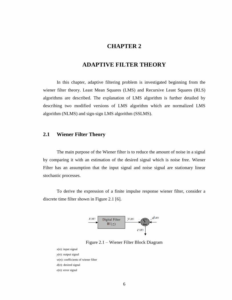
To derive the expression of a finite impulse response wiener filter, consider a
discrete time filter shown in Figure 2.1 [6].
Figure 2.1 – Wiener Filter Block Diagram
x(n): input signal
y(n): output signal
w(n): coefficients of wiener filter
d(n): desired signal
e(n): error signal

7
The output y(n) is expressed as
L-1
y(n) = ∑ wk(n)x(n-k) (2.1) k=0 or
y(n) = w(n)Tx(n) (2.2)
where x(n-k) are the input signal samples and wk are the corresponding weighting
elements for the filter coefficients. x(n) and w(n) are representing the column vectors
consisting of the x(n-k) and wk elements respectively.
The difference of desired signal d(n) and output signal y(n) is defined as error
signal e(n) [6].
e(n) = d(n) – y(n) (2.3)
The cost function J is defined as the expected value of the square of error signal
[6].
J = E{e2(n)} (2.4)
The purpose of a wiener filter is to minimize the cost function. The optimum
filter coefficients can be found by finding the minima of this cost function. Since J is a
quadratic function of the filter w(n), the gradient of the cost function with respect to w(n)
is
J = -2E{x(n-k)e(n)} k =0,1,…..L (2.5)
The necessary and sufficient condition for the cost function to attain its minimum
value is that the corresponding value of error e(n) is orthogonal to each input sample that

8
enters into the estimation of the desired response at time n. The minimum value of the
cost function is reached when gradient of the cost function is zero [6].
E{x(n-k)emin(n)} = 0 k =0,1,…..L (2.6)
where emin denotes the minimum error when the filter reaches its optimum state.
Rewriting (2.6) by using (2.1) and (2.3);
L-1
y(n) = ∑ wopt(j) E{x(n-k)x(n-j)} = E{x(n-k)d(n)}, k = 0,1,2,….L (2.7) j=0
where wopt(n) denotes the weighting function at its optimum state and L is the filter
length. Defining
r(j-k) = E{x(n-k)x(n-j)} (2.8)
p(-k) = E{x(n-k)d(n)} (2.9)
where r(j-k) is the autocorrelation function of the input signal and p(-k) is the cross-
correlation function of the input signal and the desired response, a simpler form of (2.7)
can be written as in (2.10) [6].
L-1
∑ wopt(j)r(j-k) = p(-k), k=0,1,2,….L (2.10) j=0
The matrix form of (2.10) is known as Wiener-Hopf equation and can be
rewritten as [6]
Rwopt = p (2.11)
where R is the autocorrelation matrix of input signal x(n), p is the cross-correlation
function of input signal x(n) and desired signal d(n). wopt is the vector consisting of the

9
optimum filter coefficients which minimizes E{e2(n)} known as mean squared error
(MSE).
2.2 Least Mean Square Algorithm
LMS (least mean square) is an adaptation algorithm which finds the optimal
filter coefficients minimizing instantaneous squared values of error signal. LMS
algorithm is an approximation to the steepest descent algorithm using expected value of
squared error signal. LMS is useful in applications where the entire knowledge of error
signal is not available [6].
LMS algorithm finds the filter coefficients iteratively according to (2.12)
w(n+1) = w(n) + ½µ[- J] (2.12)
where w(n+1) represents the vector consisting of the updated filter coefficients, µ is the
step size and J is the cost function. The cost function J is the instantaneous squared
value of error signal e(n).
J = e2(n) (2.13)
The gradient of the cost function is written using (2.2) and (2.3) as
e2 (n) = -2e(n)x(n) (2.14)
Therefore, the update equation of the filter coefficients is
w(n+1) = w(n) + µ[x(n)e(n)] (2.15)
where
e(n) = d(n) – y(n) (2.16)
and
10
y(n) = w(n)Tx(n) (2.17)
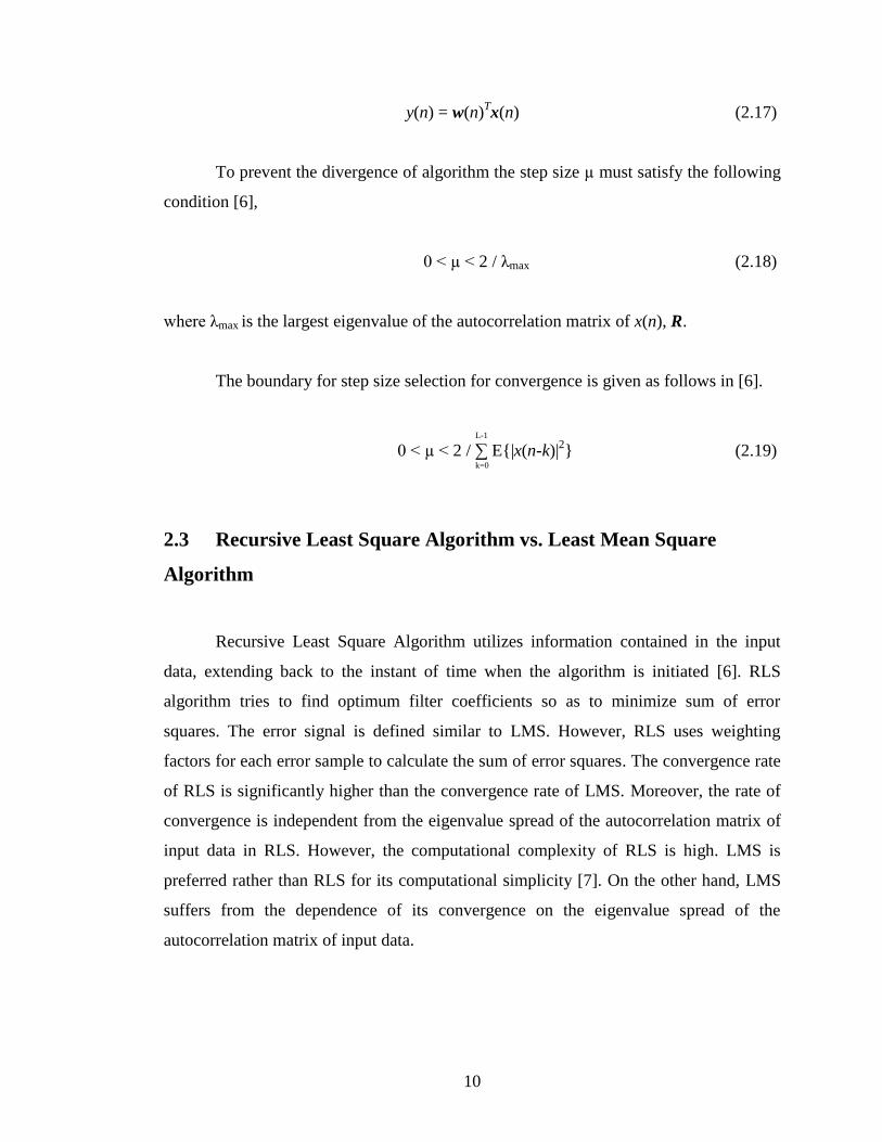
To prevent the divergence of algorithm the step size µ must satisfy the following
condition [6],
0 < µ < 2 / λmax (2.18)
where λmax is the largest eigenvalue of the autocorrelation matrix of x(n), R.
The boundary for step size selection for convergence is given as follows in [6].
L-1 0 < µ < 2 / ∑ E{|x(n-k)|
2} (2.19)
k=0
2.3 Recursive Least Square Algorithm vs. Least Mean Square
Algorithm
Recursive Least Square Algorithm utilizes information contained in the input
data, extending back to the instant of time when the algorithm is initiated [6]. RLS
algorithm tries to find optimum filter coefficients so as to minimize sum of error
squares. The error signal is defined similar to LMS. However, RLS uses weighting
factors for each error sample to calculate the sum of error squares. The convergence rate
of RLS is significantly higher than the convergence rate of LMS. Moreover, the rate of
convergence is independent from the eigenvalue spread of the autocorrelation matrix of
input data in RLS. However, the computational complexity of RLS is high. LMS is
preferred rather than RLS for its computational simplicity [7]. On the other hand, LMS
suffers from the dependence of its convergence on the eigenvalue spread of the
autocorrelation matrix of input data.
11
2.4 Modified Least Mean Square Algorithms
Considering different properties of LMS algorithms, such as stability,
convergence rate and computational requirements of implementation, various types of
LMS algorithms are developed.
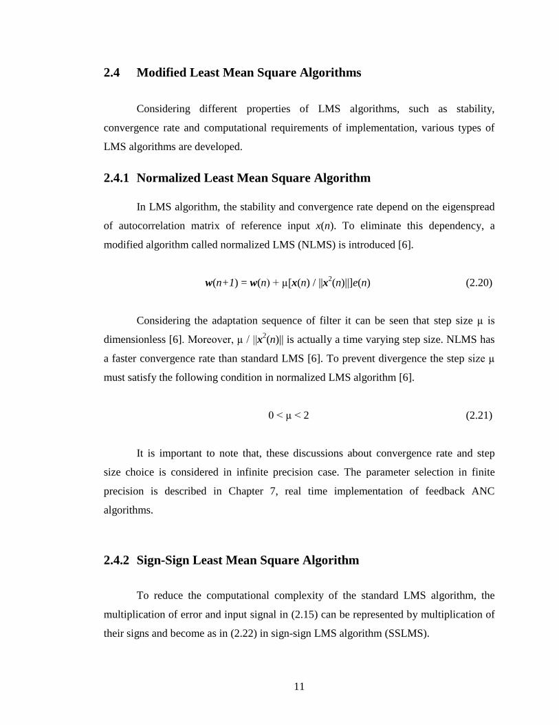
2.4.1 Normalized Least Mean Square Algorithm
In LMS algorithm, the stability and convergence rate depend on the eigenspread
of autocorrelation matrix of reference input x(n). To eliminate this dependency, a
modified algorithm called normalized LMS (NLMS) is introduced [6].
w(n+1) = w(n) + µ[x(n) / ||x2(n)||]e(n) (2.20)
Considering the adaptation sequence of filter it can be seen that step size µ is
dimensionless [6]. Moreover, µ / ||x2(n)|| is actually a time varying step size. NLMS has
a faster convergence rate than standard LMS [6]. To prevent divergence the step size µ
must satisfy the following condition in normalized LMS algorithm [6].
0 < µ < 2 (2.21)
It is important to note that, these discussions about convergence rate and step
size choice is considered in infinite precision case. The parameter selection in finite
precision is described in Chapter 7, real time implementation of feedback ANC
algorithms.
2.4.2 Sign-Sign Least Mean Square Algorithm
To reduce the computational complexity of the standard LMS algorithm, the
multiplication of error and input signal in (2.15) can be represented by multiplication of
their signs and become as in (2.22) in sign-sign LMS algorithm (SSLMS).
12
It is obvious that, convergence rate is considerably decreased in SSLMS
algorithm. To reduce computational complexity and not to decrease the convergence rate
as dramatically as in SSLMS, one can use the sign-data LMS as in (2.23) or sign-error
LMS as in (2.24) in which only one of the multiplicative factor is taken as the sign of the
signal.
w(n+1) = w(n) + µsign(x(n))sign(e(n)) (2.22)
w(n+1) = w(n) + µsign(x(n))e(n) (2.23)
w(n+1) = w(n) + µx(n)sign(e(n)) (2.24)

13
CHAPTER 3
ADAPTIVE ACTIVE NOISE CONTROL THEORY
In this chapter, feedforward and feedback ANC systems are explained. In
addition, the secondary path in ANC system, filtered input LMS algorithm and offline
secondary path modeling are described.
3.1 Feedforward Active Noise Control
In a single channel feedforward active noise control system there are two
microphones and one secondary source as seen in Figure 3.1. The reference microphone
is placed near the noise source whereas the error microphone is placed near the
secondary source. Reference signal from the reference microphone and residual error
signal from the error microphone is used for the adaptation of the filter as seen in Figure
3.2 [4].
Figure 3.1 – Feedforward Active Noise Control System Configuration

14
Figure 3.2 – Feedforward Active Noise Control System Block Diagram
d(n) : primary noise signal
x(n) : reference signal
y(n) : adaptive filter output signal
e(n) : error signal
3.2 Feedback Active Noise Control
Feedback ANC system is first proposed by Olson [3]. Since there is no reference
microphone, Feedback ANC system generates its own reference signal based on
adaptive filter output signal and error signal [4]. Feedback ANC system is required for
applications in which it is not possible to sense a reference noise signal coherent to noise
source. Headphone system in this study is based on Feedback ANC principle.

15
Figure 3.3 – Feedback Active Noise Control System Configuration
Figure 3.4 – Feedback Active Noise Control Block Diagram
d(n) : primary noise signal
y(n) : adaptive filter output signal
e(n) : error signal
Adaptive feedback ANC estimates the primary noise signal and uses it as the
reference signal [4]. As seen in Figure 3.3 and Figure 3.4 the output of the adaptive
controller is summed with noise to be reduced and the resultant signal is directly fed
back to the controller.

16
3.3 Secondary Path Transfer Function in ANC Systems
In practical implementations of ANC systems, there exist transfer paths between
digital output and digital input of adaptive controller as seen in Figure 3.5 [4].
Figure 3.5 – Block Diagram of Transfer Functions between Input and Output of
Adaptive Feedback Controller
The contribution of all of the paths in Figure 3.5 creates so-called secondary
path. The secondary path of a feedback ANC system can be seen in Figure 3.6.
Figure 3.6 – Secondary Path Model Transfer Function of Feedback ANC system
e(n) : error signal
y(n) : output signal
S(z) : secondary path transfer function

17
3.4 Filtered Input LMS Algorithm
The existence of secondary path in ANC systems necessitates the generation of
filtered input LMS algorithm (Fx-LMS). The generalized block diagram of filtered input
LMS algorithm is seen in figure 3.7 [4].
Figure 3.7 – Filtered Input LMS Algorithm Block Diagram
x(n) : input reference signal
d(n) : primary noise signal
e(n) : input error signal
y(n) : output of adaptive filter
x'(n) : adaptation input signal
Considering Figure 3.7, the output of the controller will become y'(n) which is
the filtered version of y(n) with secondary path. Thus the error signal is represented as in
(3.1) and (3.2)
e(n) = d(n) + y'(n) (3.1)
e(n) = d(n) + s(n) * y(n) (3.2)

18
Inserting (3.3) given below into (3.4) to, a different representation of error signal
is reached.
y(n) = w(n)Tx(n) (3.3)
e(n) = d(n) + s(n)*(w(n)Tx(n)) (3.4)
A modification in (3.4) leads to (3.5) and the error signal representation is
simplified as in (3.6).
e(n) = d(n) + wT(n)(s(n)*x(n)) (3.5)
e(n) = d(n) + wT(n)x'(n) (3.6)
where x'(n) is the vector consisting of adaptation input signal samples and w(n) is the
vector consisting of filter coefficients at instant n.
x'(n) = s(n) * x(n) (3.7)
s(n) = Z-1
{S(z)} (3.8)
The update equation of adaptive filter is as in (3.9)
w(n+1) = w(n) - (μ /2) . e2(n) (3.9)
Considering (3.6), the gradient of squared of error signal is as in (3.10).
e2(n) = 2e(n)x'(n) (3.10)
Inserting (3.10) in (3.9), (3.11) is reached.

19
w(n+1) = w(n) – μe(n)x'(n) (3.11)
Thus, in Fx-LMS the input reference signal to the adaptation algorithm is filtered
creating a new signal called adaptation input signal x'(n). The filter is S(z), which is the
transfer function of secondary path. The maximum value of step size μ ensuring
convergence is [4]:
μmax = 1 / Px' (L+∆) (3.12)
where Px' is the power of filtered reference signal x'(n) and ∆ is the amount of the delay
in the secondary path. Px' is represented by E{(x'(n))2}.
In Fx-LMS the system is modeled linear time invariant. A generalized form of
Fx-LMS algorithm can be seen in equation (5) of [28]. In this generalized form the
system is modeled as linear time varying. The modified Fx-LMS algorithm can be
derived from this generalized form as in equation (13) in [28]. In modified Fx-LMS
algorithm the convergence rate is increased.
3.5 Offline Secondary Path Modeling Procedure
The secondary path in ANC system should be modeled to implement Fx-LMS
algorithm. Assuming that the secondary path is linear time invariant (LTI), a finite
impulse response (FIR) filter can be chosen as the modeling filter. The impulse response
of secondary path can be estimated by a procedure similar to the process of estimation of
adaptive filter of the controller. The estimation can be done prior to the normal operation
or during the normal operation. These methods are called offline and online modeling,
respectively. In this study, offline secondary path modeling is used.
The secondary path is modeled in offline modeling procedure by sending a
wideband signal to the secondary source and comparing a filtered version of this known
20
signal by the signal picked up from the error microphone. If the adaptation algorithm for
the corresponding filter is converged then the filter can be used as a model for the
secondary path. The critical points in secondary path modeling are the necessity of wide
band frequency characteristics of the sent signal, an optimum number of iteration
ensuring convergence and proper gain settings of input and output signals. Generally,
white noise is used as the reference signal, because it includes all frequency components
equally. Some systems were tried to be implemented by wide band music signals instead
of white noise [8]. In this study, white noise is used as output signal. A block diagram of
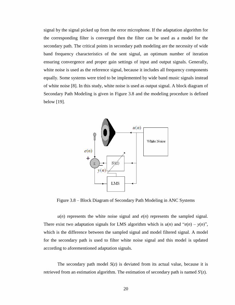
Secondary Path Modeling is given in Figure 3.8 and the modeling procedure is defined
below [19].
Figure 3.8 – Block Diagram of Secondary Path Modeling in ANC Systems
u(n) represents the white noise signal and e(n) represents the sampled signal.
There exist two adaptation signals for LMS algorithm which is u(n) and “e(n) – y(n)”,
which is the difference between the sampled signal and model filtered signal. A model
for the secondary path is used to filter white noise signal and this model is updated
according to aforementioned adaptation signals.
The secondary path model S(z) is deviated from its actual value, because it is
retrieved from an estimation algorithm. The estimation of secondary path is named S'(z).
21
Using S'(z), (3.2) and (3.7) can be rewritten as
e(n) = d(n) + s'(n) * y(n) (3.13)
x'(n) = s'(n) * x(n) (3.14)
where,
s'(n) = Z-1
{S'(z)} (3.15)
Offline secondary path modeling can be used, because even 90° phase error
between S(z) and estimation S'(z) is tolerable in the secondary path model estimation
[10].
The maximum step size ensuring convergence of filtered input LMS algorithm is
as follows [4], [11];
μmax = 1 / Px' (L+∆) (3.16)
where Px' is the power of filtered reference signal x'(n) and ∆ is the amount of the
delay in the secondary path model. Considering (3.16), the delay in secondary path is
said to affect the step size upper bound. Thus, to increase the upper bound for step size
one should decrease the physical distance between secondary source and error
microphone as much as possible.
3.6 Single Channel Feedback Active Noise Control System
Since the adaptive controller in this study is based on feedback ANC system it
will be beneficial to have a closer look at feedback ANC and give detailed block
diagrams.

22
Figure 3.9 shows the block diagram of filtered input LMS algorithm [4]. There is
no reference microphone in feedback ANC system. The absence of reference signal x(n)
is compensated with estimation of primary signal d(n), which is also not trivially
accessible. The primary signal d(n) is summed with the output of the controller. The
resultant signal is sampled by the error microphone as e(n). Thus, the estimation of
primary signal d(n) can be made by using estimation of output signal y'(n). The
estimated signal is named đ(n). The additional blocks for d(n) estimation can be seen in
Figure 3.10.
Figure 3.9 - Filtered Input LMS Algorithm Block Diagram
Figure 3.10 - Filtered Input LMS Algorithm in Feedback System with Primary Signal
Estimation Block
23
The estimated primary signal is retrieved as in (3.17) and (3.18).
đ(n) = e(n) – y'(n) (3.17)
đ(n) = e(n) – s'(n) * y(n) (3.18)
The update equation can be written as in (3.20) using (3.19).
e(n) = d(n) + wT(n) đ'(n) (3.19)
w(n+1) = w(n) - μe(n) đ'(n) (3.20)
μmax = 1 / Pđ'(L+∆) (3.21)
are reached where Pđ' is the power of filtered estimated primary signal đ'(n), L is the
order of the adaptive filter and ∆ is the amount of delay in secondary path model.
Filtered primary signal estimation đ'(n) is represented as in (3.22) where s'(n) is
secondary path model.
đ'(n) = s'(n) * đ(n) (3.22)
(3.22) can be rewritten for normalized LMS as follows:
w(n+1) = w(n) - μ e(n) đ'(n) / || đ'(n)|| (3.23)
It is critical to note that these results are not actual representations of the real
time application. Above analysis belongs to a system with no delay. A more detailed
derivation considering the delays inherent to digital implementation will be given in
Chapter 7.
24
CHAPTER 4
EFFECTS OF FINITE PRECISION ON ADAPTIVE
FILTERS
In this chapter, the effects of quantization on LMS algorithm implementation are
explored by investigating derivations made so far in literature. Moreover, another
additional problem originating from fixed point implementation is described which is
called slowdown phenomenon.
The input signal e(n) and output signal y(n) in Fx-LMS algorithm from (3.19) to
(3.22) are represented by quantized values in a digital signal processor. The procedure of
sampling and digitizing the analog signal is accomplished by analog-to-digital Converter
(ADC) devices. Similarly, a digital-to-analog converter (DAC) device produces analog
signals according to the digital words given by a digital signal processor.
In audio applications, the device containing both ADC and DAC components
within encoding, decoding, filtering and interpolation blocks are CODECs. CODECs
represent a digital word by 14 bits, 16 bits, 24 bits or 32 bits according to the precision
needed specific to application. In this study a 16-bit CODEC is used. 16-bit is sufficient
for representing input/output variables since the dynamic range supplied by this
resolution is satisfactory. Thus, the algorithm processes the 16-bit samples of input
signal and output a 16-bit word. The arithmetic operations are achieved over these 16-bit
words in a fixed-point processor. Obviously, the operations can be done by assigning
more bits to words to widen the dynamic range. Unfortunately, for higher resolution data
the processor uses much more cycles to perform adaptation algorithms. Higher CPU
clock rates mean higher power consumption which is unacceptable for portable devices.
There exist studies [15] which optimize the bit assignment procedures in fixed point

25
LMS adaptation algorithms assuring both a minimal MSE and minimal power
consumption.
Quantization error is inherent to any digital system. It is shown that adaptation
algorithms which are implemented in finite precision digital environments behave
significantly different than infinite precision (analog) implemented algorithms due to not
only quantization but some further limitations [12].
4.1 The Quantization Error of MSE in Finite Precision Adaptive
Filters
To derive an analytical expression for the quantization error, considering the
infinite precision and finite precision filters together, filter output equations will be as
follows [12]
N-1
y(n) = ∑ wk(n)x(n-k) (4.1) k=0
N-1 Ŷ(n) = ∑ Ŵk (n)x(n-k) (4.2)
k=0
where Ŷ(n) and Ŵk (n) are the corresponding digitized values of y(n) and wk(n)
respectively. The quantization error is
QE = y(n) - Ŷ(n) (4.3)
N-1
= ∑ [wk (n) - Ŵk (n)] . x(n-k) (4.4) k=0
The mean-squared QE can be written as
N-1 N-1 E{QE
2} = E{ ∑ ∑ [wk (n) - Ŵk (n)] . [wm(n) – Ŵm(n)] . x(n-k) . x(n-m)} (4.5)
k=0 m=0

26
Assuming that the inputs {xi}’s are independent random variables whose root
mean square is equal to Xrms, (4.5) can be approximated as
N-1 E{QE
2} = E{ ∑ [wk(n) - Ŵk(n)]
2. X
2rms (4.6)
m=0
≤ N. LSD2. X
2rms (4.7)
Rewriting (4.7) removing the power-of-two factors, (4.8) is reached.
QErms = N½. LSD . Xrms (4.8)
The dependence of quantization error on least significant digit value, filter length
and the input signal rms value can be seen in (4.8). The result of this derivation will be
clearer in the next section.
4.2 The Slowdown Phenomenon in Finite Precision Adaptation
The adaptation algorithms, which update the control variable in negative gradient
direction, modify the current filter vector by adding an update term. The update term is
the product of a gradient and step-size. Evidently, adaptation ceases when the update
term gets smaller in magnitude than the LSD, which is the least significant digit value of
the digitizer. This is known as the stopping phenomenon according to [12]. However, a
more detailed study shows that this effect is actually slowdown phenomenon [14].
Early termination of the adaptation or adaptation with too low speed due to
slowdown phenomenon may result in larger mean square error compared to infinite
precision case. In [13] a general derivation of the total output error is made in finite
precision case and the optimum step size value for convergence and minimum MSE is
27
said to be so small that the algorithm does not converge due to the slowdown
phenomenon.
When the update term is smaller than LSD the following equation can be written
as in [12]
| μ . eno . xno-i | ≤ LSD (4.9)
where μ is the step size and no is the time instant when the LSD value is attained by the
update term.
A further assumption that all the taps stop adapting at the same time simplifies
the relationship and replaces |xn-i| by its root mean square value, Xrms [12].
| eno | ≤ LSD / (μ.Xrms) (4.10)
ed = LSD / (μ.Xrms) (4.11)
ed is defined as the rms digital residual error (DRE). DRE is seen to be inversely
proportional to step size and root mean square value of reference signal x(n). The most
important conclusion of the DRE expression is that smaller step size values results in
larger DRE values and the step size should be larger if the adaptation stops prematurely.
In contrast, analog residual error is minimized with a smaller step size [12].
The ratio of DRE to the QE in (4.8) has important results. The ratio of DRE to
QE decreases with increasing filter length. It is important to note that longer digital
filters seem to be less sensitive to Digital Residual Error, because DRE becomes
dominant in the resultant error expression when the length of the filter is decreased.
However, increasing the filter length decreases the upper boundary of step size selection.
This smaller step size selection makes the DRE larger. Thus DRE can not be decreased
simply by decreasing the filter length. On the other hand, when the tap weights get close
28
to their optimum state the mean square error and the step size have decreased too much
and they are using very small correction terms after that point. Considering these, it can
be said that a step size decreasing in time should not be used.
In conclusion, contrary to the analog case where the error is minimized by using
a small step size, in finite precision case a smaller step size may create a larger digital
residual error due to slowdown phenomenon. Thus, there is a trade-off between
decreasing analog residual error and decreasing digital residual error. Another difference
between infinite and finite precision case is that in finite precision case a constant step
size selection made according to the aforementioned issue, gives better result then a
time-varying step size which is the optimum selection in infinite precision case [12].
Moreover, in [13] it is shown that if the number of bits used to represent the filter
coefficient is higher than the number of bits used for data inputs the dominance of the
filter length on the overall quantization error is decreased. This bit assignment proposal
is supported in [15]. In [18] equations of optimum step size selection for different
algorithms are derived in detail.
4.3 Advantage of Power-of-Two Step Size Selection in Finite
Precision
Another important issue, considering the binary digitizing environments is that
the step sizes which can be represented as power-of-two are superior because of
practical implementation considerations. In this case, multiplication with µ is usually
realized as right shifts. The error and input signals are first multiplied in double
precision; the result is then shifted and quantized to fixed point precision. The
convergence is controlled by the quantized value of the entire weight update term [16],
[17].

29
CHAPTER 5
ACTIVE NOISE CONTROL COMPUTER SIMULATIONS
Preliminary simulations should be made in a flexible environment before real
time implementation in order to gain experience about LMS algorithm, offline
secondary path modeling and filtered input LMS algorithm. The software environment is
chosen as MATLAB and the variables are represented in infinite precision for all
simulations.
5.1 Secondary Path Model Simulations
The feasibility of the practical implementation of offline secondary path
modelling is investigated. Theory is applied by creating artificial input and output
signals in offline secondary path modelling by inserting a predefined delay between
these signals. It is aimed to see whether a pure delay secondary path model S'(z) can be
estimated by the proposed adaptation process and examine the impulse response of S'(z).
In Figure 5.1, a pure delay S'(z) is estimated accurately, as the result of proper
step size selection and sufficient number of iteration. In Figure 5.2, the importance of
step size selection is seen. Step size is increased to attain a faster convergence rate.
However, the resultant S'(z) is deviated from ideal model. In Figure 5.3, another problem
which is early termination of adaptation for offline secondary path model is seen. This
problem may be visible due to slowdown phenomenon mentioned in Chapter 4. Thus the
same explanation made for the step size selection of finite precision LMS
implementation, also applies to finite precision secondary path modelling process.

30
0 5 10 15-1.2
-1
-0.8
-0.6
-0.4
-0.2
0
0.2
am
plit
ude
sample number
secondary path model of pure delay
Figure 5.1 – An Accurate Secondary Path Model Estimation of Pure Delay in MATLAB
with stepsize 1/1000
0 5 10 15-1400
-1200
-1000
-800
-600
-400
-200
0
200
am
plit
ude
sample number
secondary path model of pure delay - step size is large
Figure 5.2 – An Improper Secondary Path Model Estimation of Pure Delay in MATLAB
with stepsize 1/10000

31
0 5 10 15-5
-4
-3
-2
-1
0
1
2x 10
-3 secondary path model of pure delay - premature termination
Figure 5.3 – An Improper Secondary Path Model Estimation of Pure Delay in MATLAB
due to Insufficient Iteration
5.2 Noise Cancellation Simulations
By using the secondary path model estimation, Fx-LMS algortihm for feedback
ANC system is implemented. The acoustic superposition of primary noise signal and
secondary source output is artificially made. The crucial points about update coefficient
in adaptation equation which is discussed in Chapter 3 are investigated in detail.
In Figure 5.4, the frequency components of tonal noise input to the simulation is
seen. In Figure 5.5, it is seen that a proper step size selection and sufficient iteration
number results in convergence of the filter coefficients and the error value to decrease to
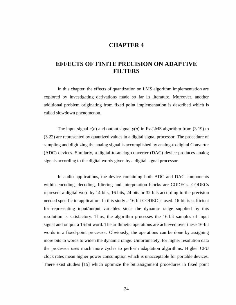
its minimum. Figure 5.6 shows the filter coefficients of this simulation. As can be seen
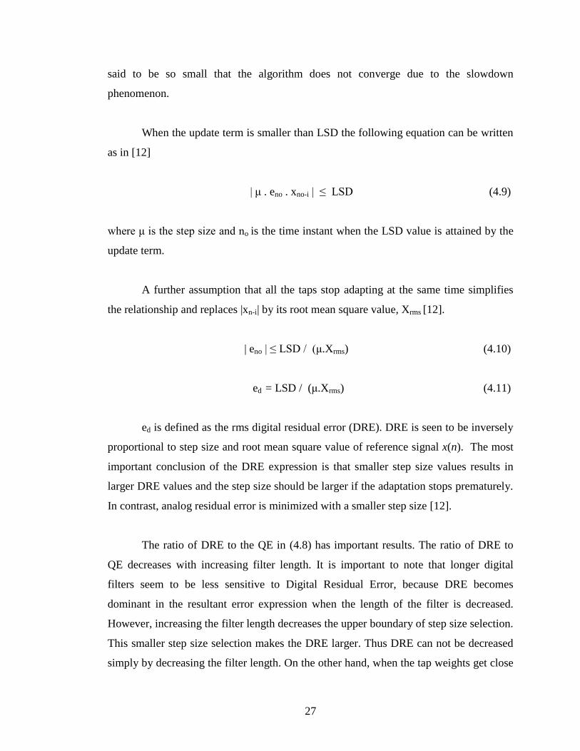
in Figure 5.7 a faster convergence can be achieved with a larger step size within the
boundary of step size selection.

32
0 500 1000 1500 2000 2500 3000 3500 40000
2
4
6
8
10
12
14x 10
4
am
plit
ude
frequency
spectral density of primary noise signal
Figure 5.4 – Fourier Transform of Primary Noise Signal in ANC Simulation in
MATLAB
0 2 4 6 8 10 12 14
x 104
-3
-2
-1
0
1
2
3
iteration number
e(n
)
Fx-LMS Feedback ANC - error value
Figure 5.5 – The Decreasing Characteristic of Error Signal by a Proper Adaptation
process due to suitable step size selection (1/10000) in MATLAB
33
0 5 10 15 20 25-0.15
-0.1
-0.05
0
0.05
0.1
0.15
0.2
Filter Taps
Am
plit
ude
The Adaptation Filter
Figure 5.6 – Adaptation Filter Coefficients of a Converged Simulation in MATLAB
0 2 4 6 8 10 12 14
x 104
-3
-2
-1
0
1
2
3
iteration number
e(n
)
Fx-LMS Feedback ANC - error value - step size value is increased
Figure 5.7 – Faster Convergence due to a Larger Step Size (1/5000) within the Boundary
of Convergence in MATLAB
An interesting result can be seen in Figure 5.8 and Figure 5.9 which shows the
importance of the accurate đ(n) retrieval. If the primary noise signal is correctly

34
retrieved, Figure 5.8 is reached. However, if one sample error is inserted in this retrieval
process, a slower convergence rate is attained as can be seen in Figure 5.9. It is also
possible to show that a more severe retrieval error may result in divergence.
0 100 200 300 400 500 600 700 800 900 1000-3
-2
-1
0
1
2
3The Error Signal vs Iteration Number - Accurate Superposition
e(n
)
Number of Iteration
Figure 5.8 – Convergence Rate with The Accurate Retrieval of Primary Noise in
MATLAB
0 100 200 300 400 500 600 700 800 900 1000-3
-2
-1
0
1
2
3The Error Signal vs Iteration Number - 1 sample delay in Superposition
e(n
)
Number of Iteration
Figure 5.9 – Slower Convergence Rate Because of The Inaccurate Retrieval of Primary
Noise in MATLAB

35
CHAPTER 6
DESIGN OF PORTABLE DIGITAL ANC HEADPHONE
SYSTEM
The portable digital ANC headphone system consists of two main parts which
are controller card and headset. There are two microphone inputs and one headphone
output on the controller card. Another input is line-in for external music sources. In this
study the external music source part is not implemented. In each ear cup of the
headphone there exists a speaker and an omnidirectional SMD active microphone biased
from the controller card. The device is compatible to work with voltages of 3.3V to 5.5V
and consumes 150mA. The system can be used actively for 15 - 20 Hours using 2300
mAh batteries.
The operation is based on feedback ANC principle. The noise existing on the
microphone diaphragm is sampled as residual error and the opposing signal sample is
sent to the headphone. The microphone is directed to the speaker resembling to the
position of the ear. The location of the microphone is experimentally decided and
stabilized. In [8] and [9] the optimum location of error microphone issue is discussed.
The headphone of the system is able to supply audio band frequencies in a flat manner
and allow a suitable location for microphone.
6.1 Schematic Design
The main block consists of Texas Instruments TLV320AIC20K CODEC, Texas
Instruments TMS320VC5416PGE120 DSP, Knowles Acoustics SP0103NC Active
Microphone and Sennheiser HD 265 Headphone. The bias voltage of Microphone is fed
36
by the CODEC through its MICBIAS output. The input signal is passed through a
bandpass filter and fed to the headset (channel-1) and handset (channel-2) inputs of
CODEC. These analog inputs are taken and digitized by CODEC. 150 Ohm Analog
outputs of the CODEC are connected to the headphone. CODEC produces analog
signals according to the digital data taken from DSP. The digital data transfer between
DSP and CODEC is accomplished by a multi channel buffered serial port working at
256 KHz. The frequency of the frame synchronization signal of this serial port is 8 KHz
which is the sampling frequency of the audio signals. The input digital data is 32-Bit
long consisting of two 16-Bit channels corresponding to each CODEC channel. The
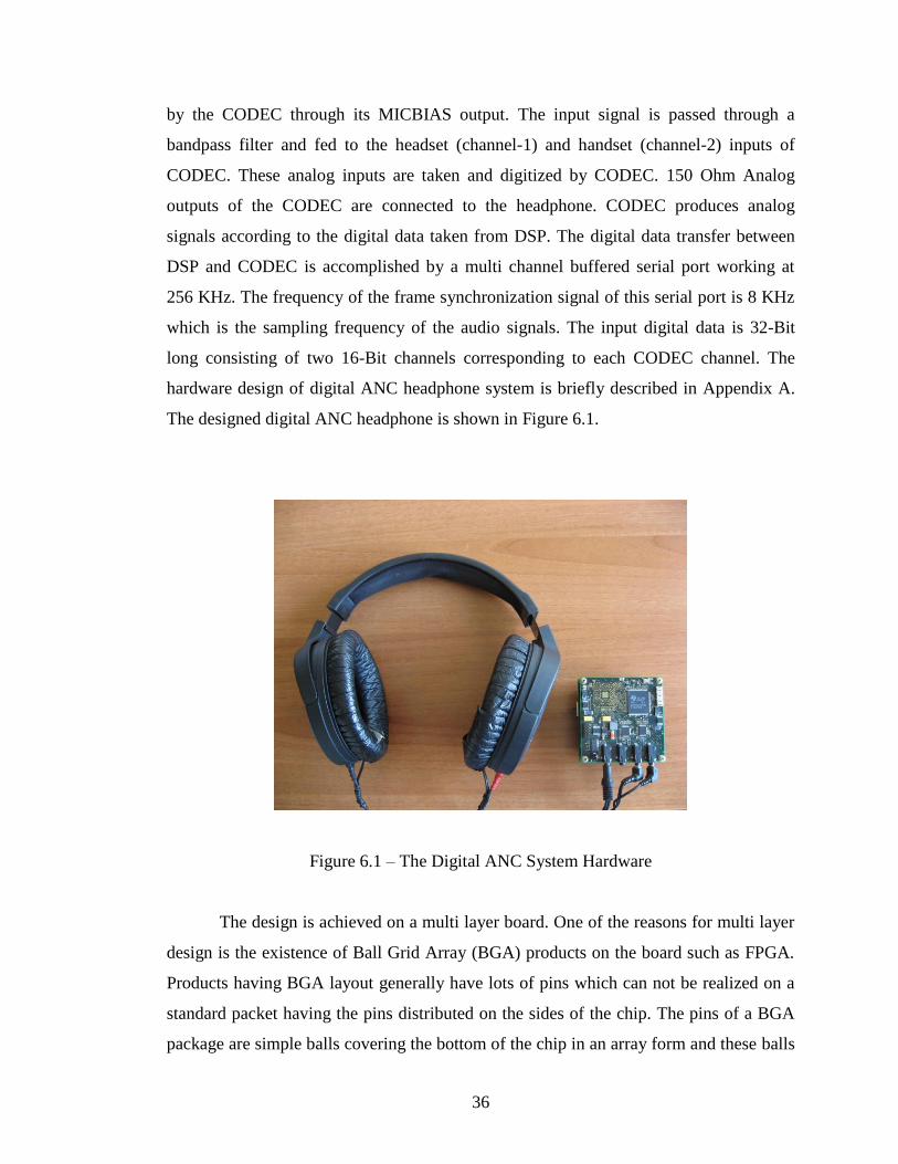
hardware design of digital ANC headphone system is briefly described in Appendix A.
The designed digital ANC headphone is shown in Figure 6.1.
Figure 6.1 – The Digital ANC System Hardware
The design is achieved on a multi layer board. One of the reasons for multi layer
design is the existence of Ball Grid Array (BGA) products on the board such as FPGA.
Products having BGA layout generally have lots of pins which can not be realized on a
standard packet having the pins distributed on the sides of the chip. The pins of a BGA
package are simple balls covering the bottom of the chip in an array form and these balls

37
are so close to each other that the interior pins can not be laid through the outer side of
the chip without crossing any line or any other ball. These should be laid on a multi-
layer card.
Another reason for multi-layer design is the necessity of stable ground and
voltage levels, which is a specific requirement of the implementation. ANC headphone
controller card carry sensitive analog and high frequency digital signals which are close
to each other. The high speed signals on the board makes transitions between the low
voltage and high voltage levels rapidly. During these transitions, there exists a current
path between each of these signal nodes to the ground. Every switching between logical
levels affects the value of the ground at the instant when the switching is occurred. The
ground value on the whole board does not change at the same time at the same level,
because each signals current finds it shortest path from its high level node to the ground.
Thus, ground levels can represent different voltages on different part of the card. An
analog signal which is generally referencing ground and near to aforementioned digital
signal path is affected. The analog signals should be isolated from digital swinging.
The most vulnerable analog signal in DSP board is the microphone signal,
because the voltage output of a microphone is so low that it can be lost as a result of the
stated ground swinging problem. Most electrets microphone suffers from this problem
since their voltage levels are in the order of 0.1 – 1mV. However, SP0103NC
microphone which is used in this system is an active SMD microphone. It has an
embedded gain stage which gives 20dB gain as pre-amplification to the output of its
transducer [27]. However, the ground swinging problem is still a problem to be solved.
To eliminate the aforementioned grounding problem and increase the noise
immunity of the system, the grounding of the card is made carefully. The problem is
solved by distinguishing the grounds for the digital and analog signals and defining a
plane for each of them through the whole card. Additionally, another main ground is
defined to which the analog and digital grounds are electrically connected at the 4
corners of the card through large vias (defined as drills through layers of the card).
38
Another solution is defining two different ground regions in the same plane.
Then, the circuits using analog ground and digital ground are laid near to analog part and
digital part respectively. These two ground parts are electrically connected to each other
through only one path. This solution has a drawback of creating an inductance between
two ground regions.
Besides distinguishing ground layers, the voltage supplies of digital devices and
analog devices are given from different regulators whose outputs are independent.
Moreover groundings of these regulators are supplied from their corresponding ground
layer.
6.2 DSP Configuration
The configuration of TMS320VC5416 DSP consists of configuration of CPU
(central processing unit) registers and some peripheral registers of the serial port
between DSP and CODEC. The register description of TMS320VC5416 is given in
Appendix B.
The implementation of the ANC system on DSP can be realized in several ways,
considering the serial port communication. In this study, specialized multi channel
buffered serial ports (McBSPs) of the DSP are used by the CPU itself. The McBSPs are
based on the standard serial-port interface found on other 54x devices [20]. The brief
description of serial ports in TMS320VC5416 is given in Appendix B. Chip support
library (CSL) of DSP is useful for configuration of DSP and signal processing
implementation. In this study, general approach is to use CSL wherever appropriate [24].
As a result of configuration of serial port of TMS320VC5416 DSP the write and
read processes should be synchronous to XRDY and RRDY signals respectively. XRDY
means transmit ready whereas RRDY means receive ready. These are indicator signals
toggling from their idle states when the corresponding buffer registers are ready to be
39
written (XRDY) or to be read (RRDY) [21]. It is crucial to wake the port from reset after
configuration and before writing to DXR register.
It is important to note that the data line carries two 16-bit channels together and
the synchronization of read/write and signal processing operation is critical. The missing
samples on each channel or the placement of each channel samples on the other channel
arrays causes the algortihm to easily diverge or the secondary path model not to be
properly estimated.
In this study, first XRDY signal is monitored by CPU. CPU waits until the DXR
register is suitable for a write, which means DXR register to XSR register copy is
accomplished. Afterwards, the data is written to DXR. Similarly when RRDY signals
that DRR register is ready to be read, the content of these register is taken by the CPU.
The details of this flow is explained in Chapter 7.
6.3 CODEC Configuration
TLV320AIC20K is a specified Texas Instrument CODEC which is optimized for
the DSPs of Texas Instrument Company [23]. The resolution of the codec is 16-bit and
sampling rate can be maximally 26 KHz. The interior architecture is based on sigma-
delta analog-to-digital and digital-to-analog converters. This CODEC carries two
independent channels having an ADC and a DAC. The gain settings in the CODEC are
critical considering the discussions made so far about secondary path model estimation
and accurate sampling of error signal in noise cancellation. These settings are adjusted
according to the experiments made with sinusoidal signals with known amplitude and
frequency. The specifications and settings of TLV320AIC20K CODEC is given in
Appendix C.

40
6.4 DSP Software for ANC Headphone System
The software starts to apply initialization of DSP’s CPU and peripheral registers.
This may be done by “gel” files in Code Composer Studio 3.1. Initial values of registers
for flash-ROM boot should be carefully assigned . One of the general purpose outputs of
DSP is dedicated for reset signal of TLV320AIC20K since a power-up process is
necessary for CODEC [23]. First CODEC is initialized. Then, the variables that will be
used in following blocks are initialized and the McBSP is configured for CODEC
configuration. The CODEC configuration words are written and checked according to
[23] and the two main blocks of algorithm start to run consecutively: Offline Secondary
Path Modeling and Fx-LMS Adaptive Noise Cancellation Algorithm.
Figure 6.2 shows the main blocks in DSP software. This block diagram does not
contain low-level processes such as program loading from flash-ROM or emulator.
Figure 6.2 – Generalized Block Diagram of the DSP Code for Fx-LMS Adaptive ANC
Headphone System

41
CHAPTER 7
REAL TIME FEEDBACK ACTIVE NOISE CONTROL
IMPLEMENTATION
In this chapter software implementation of feedback ANC and offline secondary
path modeling are described. The delays existing between digital and analog parts of the
controller are represented. The algorithm implementation is modified considering the
effects of these delays. The step size selection of LMS algorithm is made considering
fixed point implementation. Moreover, software adjustments are proposed to overcome
practical problems. One of these problems is changing of secondary path when the
headphone is put off. The other problem is divergence of the algorithm when a dynamic
range exceeding noise is applied to the system.
7.1 A Practical Approach about Delays in Fx-LMS in ANC
Application
There exist delays between digital and analog parts of the ANC system. One of
the reasons for these delays is the buffered communication structure between DSP and
CODEC. The other reasons are the analog-to-digital and digital-to-analog conversion
times of CODEC and the acoustic delays. These delays should be examined, because
they affect the update equation of adaptive filter and estimation of primary signal. The
actuation component of update equation is the multiplication of stepsize and negative
gradient of squared error signal as seen in (7.1).
w(n+1) = w(n) - (μ /2) . e2(n) (7.1)

42
The residual error sample e(n) is created by the summation of output of adaptive
filter and primary noise signal. The output of adaptive filter is not output from the
secondary source just after it is created because of the aforementioned delays. Moreover,
the error sample taken into DSP actually belongs to earlier sampling instants because of
these delays. In order to calculate the gradient of squared error signal correctly, these
delays should be considered. To understand the effects of these delays mathematically,
consider the analog signal e(t) and its sampling operation in Figure 7.1 and remember
the block diagram of filtered input LMS algorithm in feedback system seen in Figure
7.2.
Figure 7.1 - The Sampling of Error Signal in Real Time Implementation of ANC
Headphone System
Figure 7.2 - Filtered Input LMS Algorithm in Feedback System
43
Assume that, A is the delay amount in receive path from microphone to DSP
including acoustic delay between noise signal and transducer. Similarly assume that, B
is the delay amount in transmit path from DSP to speaker including the delay of the
speaker. The delay amount in secondary path model s(n) was defined as ∆ in Chapter 3.
It is evident that ∆ is summation of A and B.
nA means a time instant after the present time by an amount A, similarly n-B
means a time instant before the present time by an amount B. At n = nA, e(n0) is
sampled, because of the delays between microphone and DSP. At n = n-B output sample
y(n-B) was created and given to the CODEC. y(n-B) was turned into analog signal at n =
n0 because of the delays between DSP and speaker. Thus, e(n0) was created with
contribution of primary noise sample d(n0) and y(n-B).
e(n0) = d(n0) + y(n-B) (7.2)
At n = nA, đ(n0) can be estimated as in (7.3).
đ(n0) ≈ d(n0) = e(n0) - y(n-B) (7.3)
w(nA) in (7.4) represents the adaptive filter coefficients at instant nA. y(n-B) can be
calculated as in (7.5).
y(nA) = w(nA)T đ(n0) (7.4)
y(n-B) = w(n-B)T đ(n-(A+B)) (7.5)
Thus, (7.2) can be rewritten as in (7.6).
e(n0) = d(n0) + w(n-B) T
đ(n-(A+B)) (7.6)
The update equation at n = nA is as in (7.7).

44
w(nA+1) = w(nA) – (μ/2). J (7.7)
where J = e2(nA) and w(nA+1) represents the filter coefficients which will be used for the
following cycle. Rewriting (7.7) using (7.8), (7.9) is reached.
J = 2.e(nA). đ(n-(A+B)) (7.8)
w(nA+1) = w(nA) - μ. e(n0). đ(n-(A+B)) (7.9)
w(nA) in (7.9) is updated with the error signal resulted from the output signal at
instant n-B as seen in (7.3). This output sample is created by w(n-B). This result is
inevitable because of the delays existing between input and output signal of digital
controller.
The filtered primary signal estimation signal is delayed in modified update
equation (7.9). The secondary path model compensates for these delays in update
equation, because the delay amount of secondary path model is the summation of A and
B. Thus, rewriting (7.9) using đ'(n0), (7.10) is reached. đ'(n) is the convolution of
secondary path model s(n) and estimated primary signal đ(n). đ'(n) is the array
consisting of the filtered estimated primary signal samples.
w(nA+1) = w(nA) - μ. e(n0). đ'(n0) (7.10)
Although the update equation is not affected by aforementioned delays, the
estimation of primary signal should be made considering these delays. The delay
between DSP and speaker should be taken into account as seen in (7.3). The effect of
one sample estimation mistake on the convergence rate is clearly seen in Chapter 5,
Figure 5.8 and Figure 5.9. The estimation of primary signal can be made by using the
secondary path filtered y'(n0) instead of y(n-B) as in (3.18) if A is small enough with
respect to changes in output signal y(n). Both of y'(n0) and y(n-B) are tried experimentally

45
in this study and it is seen that there is no significant difference in performance of these
implementations.
7.2 The Software Architecture of Fx-LMS ANC
Considering the derivations made for the delays in real time ANC, the following
equations are used to realize the feedback ANC in this study.
y(n) = wT(n).đ(n)
y'(n) = s'T(n).y(n)
đ(n) = e(n) - y'(n)
đ'(n) = s'T (n).đ(n)
w(n+1) = w(n) – μ. e(n).đ'(n)
đ(n) and y(n) vectors are input and output arrays which are used for convolution with
filters. đ'(n) is the vector consisting of filtered estimated primary signal samples. Several
experiments are made to decide on the filter length. 128 Tap filters are decided to be
used for secondary path model s'(n) and adaptation filter w(n) in implementation of
ANC headphone system. The initial values of w(n) and s'(n) are all zeros.
The filtering operations are achieved by FIR function of chip support library
(CSL) in TMS320C54x. FIR uses circular addressing modes. In circular addressing, k+1
LSB’s of a circular buffer’s starting address must be zero where k = log2 (circular buffer
size). Memory alignment should be applied to corresponding arrays in “linker command
file” of the project developed in Code Composer Studio 3.1, which is the software
environment used in this study. The details of FIR function can be found in [22].
Generally speaking, FIR function achieves convolution of two arrays and stores the
result in an output array. The necessary CPU clock cycle for a convolution operation in
FIR function is optimized.
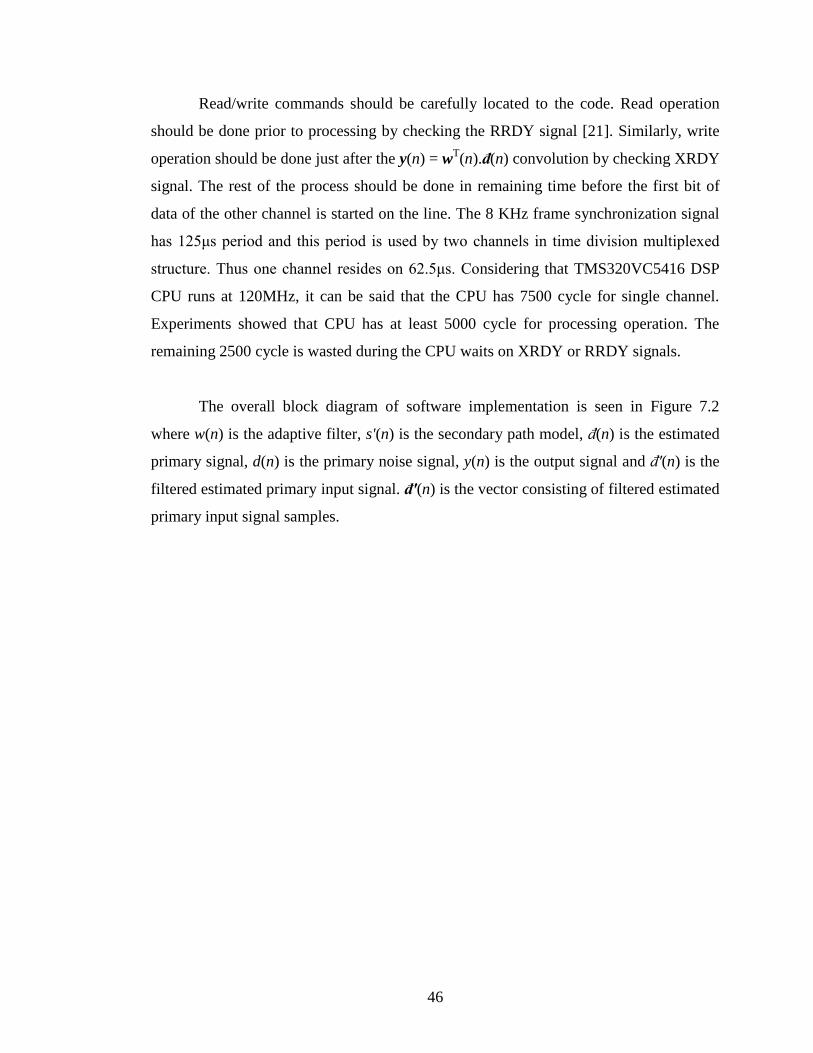
46
Read/write commands should be carefully located to the code. Read operation
should be done prior to processing by checking the RRDY signal [21]. Similarly, write
operation should be done just after the y(n) = wT(n).đ(n) convolution by checking XRDY
signal. The rest of the process should be done in remaining time before the first bit of
data of the other channel is started on the line. The 8 KHz frame synchronization signal
has 125μs period and this period is used by two channels in time division multiplexed
structure. Thus one channel resides on 62.5μs. Considering that TMS320VC5416 DSP
CPU runs at 120MHz, it can be said that the CPU has 7500 cycle for single channel.
Experiments showed that CPU has at least 5000 cycle for processing operation. The
remaining 2500 cycle is wasted during the CPU waits on XRDY or RRDY signals.
The overall block diagram of software implementation is seen in Figure 7.2
where w(n) is the adaptive filter, s'(n) is the secondary path model, đ(n) is the estimated
primary signal, d(n) is the primary noise signal, y(n) is the output signal and đ'(n) is the
filtered estimated primary input signal. đ'(n) is the vector consisting of filtered estimated
primary input signal samples.
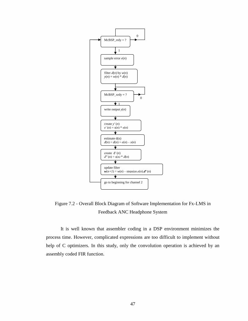
47
Figure 7.2 - Overall Block Diagram of Software Implementation for Fx-LMS in
Feedback ANC Headphone System
It is well known that assembler coding in a DSP environment minimizes the
process time. However, complicated expressions are too difficult to implement without
help of C optimizers. In this study, only the convolution operation is achieved by an
assembly coded FIR function.
McBSP_rrdy = ?
sample error e(n)
filter đ(n) by w(n) y(n) = w(n) * đ(n)
McBSP_xrdy = ?
write output y(n)
create y' (n)
y' (n) = s(n) * y(n)
estimate d(n)
đ(n) = d(n) = e(n) – y(n)
create đ' (n)
đ'' (n) = s(n) * đ(n)
update filter
w(n+1) = w(n) – stepsize.e(n).đ' (n)
go to beginning for channel 2
0
1
0
1
48
7.3 Fixed Point Limitations in LMS Active Noise Control
Implementation
Fixed point limitations affect the step size selection in LMS algorithm.
Additionally, software implementation of LMS includes some multiplication and
division operation which can produce overflow or rounding errors in finite precision
environment.
The resolution for the variables are chosen as 16-bit for input and output signals
according to the CODEC digital data format. In order to prevent some additional
unexpected error, all the other variables are defined in 16-bit resolution. The
multiplications in DSP are done using a 40-bit accumulator. The multiplication of two
16-bit integers results in a 32-bit integer. Summation of these 32-bit integers may need
higher order bits. The 40-Bit accumulator is split into three parts which are guard bits,
high order bits and low order bits. Guard bits (most significant 8 bits) are used for the
filtering operation including multiplication and addition of long filter coefficients. The
result of a multiplication is most accurate if the high order 16 bits are returned as the
result.
Division operation in fixed point is different than multiplication, because the
rounding error is produced by division. Rounding error may seem to be solved by pre-
multiplications but the upper dynamic limit of defined resolution generally puts a
restriction on the multiplication results. To prevent this, it must be ensured that the prior
multiplications are done in 40-bit accumulator and division is operated on the high
resolution value before it is normalized to 16-bit.
There exist multiplications in update equation (7.11). Although, the step size is
seen to be multiplied with the other components, it is generally a dividing factor. For
strong primary signals the upper boundary for step size selection is too small.

49
w(n+1) = w(n) - µ đ'(n) e(n)
= w(n) -[ đ'(n) . e(n) ] / [1/ µ] (7.11)
The upper boundary on the step size is determined by calculating the power of
filtered primary signal estimation đ'(n) (3.22). The signed 16-bit integer values are
between -32768 and 32767. Experiments showed that upper bound on step size is around
1/1000000 for a strong sinusoidal whose peak-to-peak amplitude value is 20000. The
multiplication of filtered estimated primary sample and error sample should be divided
by 1000000 in order to realize that step size value; however this division factor can not
be represented in 16-bit resolution. The following equation can be used although there
exists round-off error;
w(n+1) = w(n) - µ đ'(n) e(n)
= w(n) -[đ'(n) / C1 ] . [ e(n) / C2 ] (7.12)
where C1.C2 = 1/µ.
C1 and C2 can be represented in 16-bit resolution correctly. Each division result
should be kept as 16-bit integers independently and the multiplication should be done
with these division results.
If C2 is selected too high in (7.12) in order to guarantee the convergence, the
error signals smaller than this high threshold stop adaptation temporarily. Digital
residual error becomes dominant with respect to quantization error due to the slowdown
phenomenon defined in Chapter 4. C1 and C2 should be selected by experimental results
so that convergence for strong primary noise signals is ensured and weak primary noise
signals do not result in high digital residual error. If the value of C1 or C2 can not satisfy
these requirements, one should alter the gain settings of microphone input and/or
speaker output.

50
C1 and C2 are selected as 2048 (211
) in LMS algorithm in order to realize the
division by shifting the binary value of e(n) and đ'(n). C1 constant in (7.12) becomes
power of đ'(n) signal in NLMS. The initial C1 is chosen as 2048 in NLMS. Afterwards,
the squared value of the bottom element of đ'(n) array is subtracted from C1 and the new
incoming sample is added to it. C2 is also chosen as 2048 in NLMS. In SSLMS, the filter
coefficients are increased or decreased by 1 according to the signs of error and filtered
estimated primary noise signal. A dead zone of 1024 is inserted for e(n) signal in order
to prevent the sign-sign LMS algorithm to update the filter coefficients for too small
residual error signals. Inside aforementioned dead zone the filter coefficients are not
updated.
C1 and C2 are selected considering the input/output signal levels in several
experiments. These experiments showed that C2 and/or C1 value should follow an
adaptive way to maximize the dynamic range, because a strong primary noise signal
needs a smaller step size for convergence and smaller step size values increase the digital
residual error for smaller primary signals due to slowdown phenomenon. This makes the
overall ANC system ineffective for low level noise signals or divergent for high level
primary noises.
7.4 The Discussion of Modified LMS Algorithms in Fixed Point
Normalized LMS has an adaptive step size effective to both low level and high
level primary noise signals. The value of aforementioned divider factor (C1.C2) is
increased with increasing primary noise signal level. However, time-varying stepsize is a
drawback for NLMS in fixed point implementation considering discussions made in
Chapter 4. On the other hand, in NLMS the power of filtered estimated primary signal
should be calculated. The multiplication and addition operation during this calculation
results in overflow errors if the samples of estimated primary signal are not normalized
to a lower level. Since the power of filtered estimated primary signal is a dividing factor,

51
an overflow error results in divergence. The main advantage of NLMS is its increased
rate of convergence as seen in theoretical explanations in Chapter 2.
Convergence rate is decreased in sign-sign LMS. The main advantage of sign-
sign LMS is that a higher reduction than the other algorithms can be attained for weaker
signals by introducing a smaller dead zone.
7.5 Software Implementation of Offline Secondary Path Modeling
Offline secondary path modeling is implemented according to explanations made
in Chapter 3. Fixed point limitations also apply to secondary path modeling. Gain
settings and iteration number are optimized for the most accurate modeling. White noise
samples are created by random generator function in DSP library. The result of this
function is scaled and biased according to some experimental results guaranteeing the
convergence.
The block diagram of offline secondary path modeling is seen in Figure 7.3

52
Figure 7.3 – Block Diagram of Software Realization of Offline Secondary Path
Modeling in ANC Headphone System
A similar step size selection procedure to LMS implementation is followed.
s(n+1) = s(n) + [ out(n) / C1 ] . [ e(n) / C2 ] (7.13)
is reached where out(n) is the output white noise signal. As the result of several
experiments, both C1 and C2 are chosen as 2048. Offline secondary path modeling lasts
McBSP_rrdy = ?
sample input in(n)
create output
out(n) = (rand( ) -16384 / 8)
McBSP_xrdy = ?
write output
out(n)
filter out(n) by secondary path model
out_off(n) = s(n) * out(n)
create error signal
e(n) = in(n) – out_off(n)
update secondary path model
s'(n+1) = s'(n) – stepsize.e(n).out (n)
go to beginning for channel 2
0
1
0
1

53
for 10 seconds in this implementation. Figure 7.4 shows the impulse response of
secondary path model of one channel obtained in real time experiments.
Figure 7.4 – The impulse response of Secondary Path Model of Active ANC Headphone
System
7.6 Additional Software Implementations
The designed digital ANC system may loose its stability when these two
conditions occur:
A large primary noise signal exceeding dynamic range of digital ANC system is
applied.
The secondary path is changed when user puts off the headphone.
The first problem is solved by increasing the high level threshold. This is done
by decreasing the gain of the microphone. However, this resulted in the degradation in
the sensitivity of the system to low level noises. Another solution to this problem is to
automatically control the gain of the input by modifying the ADC gain settings of the
54
CODEC. However, this results in the changing of the secondary path model which
should be compensated with a new modeling. Unfortunately, it is impossible to stop the
system and make another offline secondary path modeling. CODEC should be reset and
all registers should be reconfigured with a cost of 10 samples for each channel. An
adaptive step size selection procedure is tried in order to increase dynamic range. The
step size value is decreased when the estimated primary noise power decreased below a
predefined limit. Similarly step size value is increased when estimated primary noise
power increased above a predefined limit. This adjustment is difficult to implement
because of its computational complexity.
In this study the second problem is solved by a software machine which handles
the task of checking error signal and resets the corresponding channel’s parameters
when a predefined range is exceeded by error signal. By this adjustment, the stability is
rearranged if the headphone is put on again.
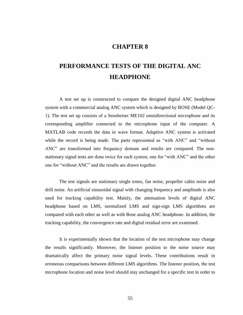
55
CHAPTER 8
PERFORMANCE TESTS OF THE DIGITAL ANC
HEADPHONE
A test set up is constructed to compare the designed digital ANC headphone
system with a commercial analog ANC system which is designed by BOSE (Model QC-
1). The test set up consists of a Sennheiser ME102 omnidirectional microphone and its
corresponding amplifier connected to the microphone input of the computer. A
MATLAB code records the data in wave format. Adaptive ANC system is activated
while the record is being made. The parts represented as “with ANC” and “without
ANC” are transformed into frequency domain and results are compared. The non-
stationary signal tests are done twice for each system; one for “with ANC” and the other
one for “without ANC” and the results are drawn together.
The test signals are stationary single tones, fan noise, propeller cabin noise and
drill noise. An artificial sinusoidal signal with changing frequency and amplitude is also
used for tracking capability test. Mainly, the attenuation levels of digital ANC
headphone based on LMS, normalized LMS and sign-sign LMS algorithms are
compared with each other as well as with Bose analog ANC headphone. In addition, the
tracking capability, the convergence rate and digital residual error are examined.
It is experimentally shown that the location of the test microphone may change
the results significantly. Moreover, the listener position to the noise source may
dramatically affect the primary noise signal levels. These contributions result in
erroneous comparisons between different LMS algorithms. The listener position, the test
microphone location and noise level should stay unchanged for a specific test in order to

56
minimize these errors. Additionally, the test microphone should be as close as possible
to the error microphone of digital ANC.
8.1 Single Tone Experiments
Figure 8.1 shows the error signal recorded during a single tone NLMS digital
ANC headphone experiment. Higher amplitudes (amplitude of power of error signal)
belong to the part “without ANC” and the lower amplitudes belong to the part “with
ANC”. The single frequency component of the test noise is 200Hz. Fourier transform of
the samples between 0 and 10000 is plotted in Figure 8.2 and the Fourier transform of
the samples between 90000 and 100000 is plotted in Figure 8.3. The attenuation level of
200 Hz single tone is 25.5 dB (10.log (434.0245 / 1,225)).
0 1 2 3 4 5 6 7 8 9 10
x 104
-0.5
-0.4
-0.3
-0.2
-0.1
0
0.1
0.2
0.3
0.4
0.5Single 200 Hz Tone - Error Signal - NLMS
am
plit
ude -
linear
scale
sample number
Figure 8.1 – Single 200 Hz Tone in NLMS Experiment “with ANC” and “without ANC”

57
Figure 8.2 – Fourier Transform of Single 200 Hz Tone in NLMS Experiment “without
ANC”
Figure 8.3 – Fourier Transform of Single 200 Hz Tone in NLMS Experiment “with
ANC”
Similar experiments are made with NLMS, LMS and SSLMS for other single
tone signals from 100Hz up to 1100 Hz for. Additionally, the Bose ANC headphone is
tested with these signals. The results of ANC experiments with single tones for different
0 500 1000 1500 2000 2500 3000 3500 4000 0
50
100
150
200
250
300
350
400
450
X= 197.5802 Y= 434.0245
frequency in Hertz
am
plit
ud
e -
line
ar
scale
Fourier Transform of Single 200 Hz Tone - without ANC
0 500 1000 1500 2000 2500 3000 3500 4000 0
0.2
0.4
0.6
0.8
1
1.2
1.4
X= 197.5802 Y= 1.225
Fourier Transform of Single 200 Hz Tone - with NLMS ANC
am
plit
ud
e -
lin
ear
scale
frequency in Hertz

58
LMS algorithms and analog ANC headphone is shown in Table 8.1. It is important to
note that the attenuation levels may significantly change (about 5-6 dB) with a change in
the location of test microphone.
Table 8.1 – The attenuation levels of single tones for digital and analog system
ANC system
frequency
Digital ANC
Headphone -
NLMS
Digital ANC
Headphone –
LMS
Digital ANC
Headphone –
Sign-Sign
LMS
Analog ANC
Headphone
100Hz 33.5 dB 28.6 dB 30.1 dB 14.6 dB
200Hz 25.5 dB 30.6 dB 21.2 dB 11.9 dB
300Hz 29.7 dB 24.0 dB 30.0 dB 10.4 dB
400Hz 24.0 dB 30.1 dB 21.5 dB 14.1 dB
500Hz 22.1 dB 31.4 dB 21.5 dB 6.5 dB
600Hz 19.0 dB 20.0 dB 18.9 dB 3.6 dB
700Hz 19.8 dB 21.1 dB 18.8 dB 1.5 dB
800Hz 18.4 dB 16.5 dB 17.3 dB -1.8 dB
900Hz 14.9 dB 24.8 dB 28.9 dB -4.3 dB
1000Hz 16.2* dB 14.7 dB* 12.9 dB* -5.4 dB
1100Hz 10.8* dB 16.0 dB* 7.3 dB* -4.7 dB
*for these frequencies the attenuation levels are not stable.
These single tone experiments show that digital ANC headphone system is
considerably superior to the analog ANC headphone system when the noise is narrow
band. Analog ANC headphone system increases frequency components higher than
700Hz - 800Hz. In contrast, digital ANC system can extend the attenuation band up to
1000Hz successfully. Furthermore, digital ANC is successful in narrowband signals in
the optimized working region of analog headphone which resides between 100Hz and

59
400Hz. LMS showed the most successful results of all the other algorithms. This is a
result of the constant step size optimizing the implementation for fixed point
environment [12].
8.2 Multiple Tone Experiments
Figure 8.4, Figure 8.5, Figure 8.6 and Figure 8.7 show the results of the
experiments made with digital ANC headphone NLMS method for the multi tone of
100Hz, 200Hz, 300Hz, 400Hz and 500Hz composition. The attenuation levels are
calculated as 17.3dB for 100Hz, 33.5 dB for 200Hz, 24.1dB for 300Hz, 28.5dB for
400Hz and 21.7 dB for 500 Hz. In Figure 8.8, Figure 8.9 and Figure 8.10, the
corresponding results for LMS, SSLMS and analog ANC headphone can be seen
respectively.
0 0.2 0.4 0.6 0.8 1 1.2 1.4 1.6 1.8 2
x 105
-0.4
-0.3
-0.2
-0.1
0
0.1
0.2
0.3
0.4
0.5
0.6Single Tone of 100Hz + 200Hz + 300Hz + 400Hz + 500Hz - with NLMS ANC
sample number
am
plit
ude -
linear
scale
Figure 8.4 - Tone of 100 Hz, 200Hz, 300Hz, 400Hz and 500 Hz Composition in NLMS
Experiment “with ANC” and “without ANC”

60
Figure 8.5 – Fourier Transform of 100 Hz, 200Hz, 300Hz, 400Hz and 500 Hz
Composition in NLMS Experiment “without ANC”
Figure 8.6 – Fourier Transform of 100 Hz, 200Hz, 300Hz, 400Hz and 500 Hz
Composition in NLMS Experiment “with ANC”
0 500 1000 1500 2000 2500 3000 3500 4000 0
10
20
30
40
50
60
Fourier Transform of 100 Hz + 200 Hz + 300 Hz + 400 Hz + 500 Hz - without ANC
am
plit
ud
e -
line
ar
scale
frequency in Hertz
0 500 1000 1500 2000 2500 3000 3500 4000 0
0.2
0.4
0.6
0.8
1
1.2
1.4
Fourier Transform of 100 Hz + 200 Hz + 300 Hz + 400 Hz + 500 Hz - with NLMS ANC
am
plit
ud
e -
line
ar
scale
frequency in Hertz
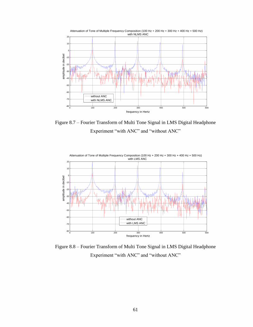
61
Figure 8.7 – Fourier Transform of Multi Tone Signal in LMS Digital Headphone
Experiment “with ANC” and “without ANC”
Figure 8.8 – Fourier Transform of Multi Tone Signal in LMS Digital Headphone
Experiment “with ANC” and “without ANC”
0 100 200 300 400 500 600 -80
-70
-60
-50
-40
-30
-20
-10
0
10
20
frequency in Hertz
am
plit
ude in d
ecib
el
Attenuation of Tone of Multiple Frequency Composition (100 Hz + 200 Hz + 300 Hz + 400 Hz + 500 Hz) with NLMS ANC
without ANC with NLMS ANC
0 100 200 300 400 500 600 -80
-70
-60
-50
-40
-30
-20
-10
0
10
20
frequency in Hertz
am
plit
ud
e in
decib
el
Attenuation of Tone of Multiple Frequency Composition (100 Hz + 200 Hz + 300 Hz + 400 Hz + 500 Hz) with LMS ANC
without ANC with LMS ANC

62
Figure 8.9 – Fourier Transform of Multi Tone Signal in Sign-Sign LMS Digital
Headphone Experiment “with ANC” and “without ANC”
Figure 8.10 – Fourier Transform of Multi Tone Signal in Analog ANC Headphone
Experiment “with ANC” and “without ANC”
The results of multi tone experiments are listed in Table 8.2. Similar experiments
are made for various multi tones and the results are shown in Table 8.3 for 200Hz,
600Hz and 800Hz composition and in Table 8.4 for 100Hz, 400Hz and 900Hz
composition.
0 100 200 300 400 500 600 -80
-70
-60
-50
-40
-30
-20
-10
0
10
20
frequency in Hertz
am
plit
ud
e in
decib
el
Attenuation of Tone of Multiple Frequency Composition (100 Hz + 200 Hz + 300 Hz + 400 Hz + 500 Hz) with Sign Sign LMS ANC
without ANC with Sign Sign LMS
0 100 200 300 400 500 600 -80
-70
-60
-50
-40
-30
-20
-10
0
10
20
frequency in Hertz
am
plit
ud
e in
decib
el
Attenuation of Tone of Multiple Frequency Composition (100 Hz + 200 Hz + 300 Hz + 400 Hz + 500 Hz) with Analog ANC Headphone
without ANC with Analog ANC Headphone
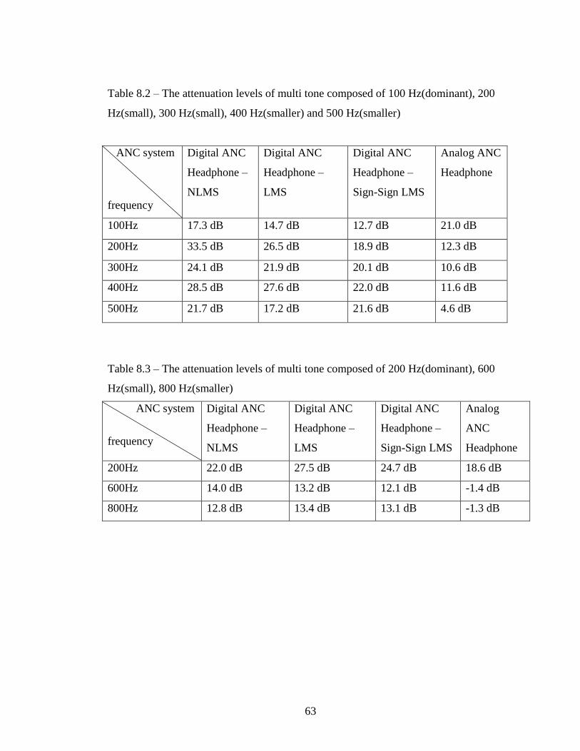
63
Table 8.2 – The attenuation levels of multi tone composed of 100 Hz(dominant), 200
Hz(small), 300 Hz(small), 400 Hz(smaller) and 500 Hz(smaller)
ANC system
frequency
Digital ANC
Headphone –
NLMS
Digital ANC
Headphone –
LMS
Digital ANC
Headphone –
Sign-Sign LMS
Analog ANC
Headphone
100Hz 17.3 dB 14.7 dB 12.7 dB 21.0 dB
200Hz 33.5 dB 26.5 dB 18.9 dB 12.3 dB
300Hz 24.1 dB 21.9 dB 20.1 dB 10.6 dB
400Hz 28.5 dB 27.6 dB 22.0 dB 11.6 dB
500Hz 21.7 dB 17.2 dB 21.6 dB 4.6 dB
Table 8.3 – The attenuation levels of multi tone composed of 200 Hz(dominant), 600
Hz(small), 800 Hz(smaller)
ANC system
frequency
Digital ANC
Headphone –
NLMS
Digital ANC
Headphone –
LMS
Digital ANC
Headphone –
Sign-Sign LMS
Analog
ANC
Headphone
200Hz 22.0 dB 27.5 dB 24.7 dB 18.6 dB
600Hz 14.0 dB 13.2 dB 12.1 dB -1.4 dB
800Hz 12.8 dB 13.4 dB 13.1 dB -1.3 dB
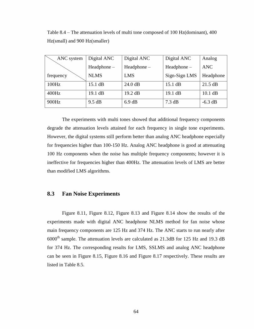
64
Table 8.4 – The attenuation levels of multi tone composed of 100 Hz(dominant), 400
Hz(small) and 900 Hz(smaller)
ANC system
frequency
Digital ANC
Headphone –
NLMS
Digital ANC
Headphone –
LMS
Digital ANC
Headphone –
Sign-Sign LMS
Analog
ANC
Headphone
100Hz 15.1 dB 24.0 dB 15.1 dB 21.5 dB
400Hz 19.1 dB 19.2 dB 19.1 dB 10.1 dB
900Hz 9.5 dB 6.9 dB 7.3 dB -6.3 dB
The experiments with multi tones showed that additional frequency components
degrade the attenuation levels attained for each frequency in single tone experiments.
However, the digital systems still perform better than analog ANC headphone especially
for frequencies higher than 100-150 Hz. Analog ANC headphone is good at attenuating
100 Hz components when the noise has multiple frequency components; however it is
ineffective for frequencies higher than 400Hz. The attenuation levels of LMS are better
than modified LMS algorithms.
8.3 Fan Noise Experiments
Figure 8.11, Figure 8.12, Figure 8.13 and Figure 8.14 show the results of the
experiments made with digital ANC headphone NLMS method for fan noise whose
main frequency components are 125 Hz and 374 Hz. The ANC starts to run nearly after
6000th
sample. The attenuation levels are calculated as 21.3dB for 125 Hz and 19.3 dB
for 374 Hz. The corresponding results for LMS, SSLMS and analog ANC headphone
can be seen in Figure 8.15, Figure 8.16 and Figure 8.17 respectively. These results are
listed in Table 8.5.

65
0 0.2 0.4 0.6 0.8 1 1.2 1.4 1.6 1.8 2
x 105
-0.05
-0.04
-0.03
-0.02
-0.01
0
0.01
0.02
0.03
0.04Fan Noise - with NLMS
am
plit
ude -
linear
scale
sample number
Figure 8.11 - Fan Noise in NLMS Experiment “with ANC” and “without ANC”
Figure 8.12 – Fourier Transform of Fan Noise in NLMS Experiment “without ANC”

66
Figure 8.13 – Fourier Transform of Fan Noise in NLMS Experiment “with ANC”
Figure 8.14 - Fourier Transform of Fan Noise in NLMS Experiment “with ANC” and
“without ANC”
100 200 300 400 500 600
-0.01
0
0.01
0.02
0.03
0.04
X= 124.5292 Y= 0.0068499
frequency in Hertz
am
plit
ud
e -
line
ar
scale
Fourier transform of Fan Noise - with NLMS ANC
0 100 200 300 400 500 600 700 800 900 -100
-90
-80
-70
-60
-50
-40
-30
-20
-10
0
frequency in Hertz
am
plit
ud
e in
decib
el
Attenuation of Fan Noise with NLMS ANC
without ANC with NLMS ANC
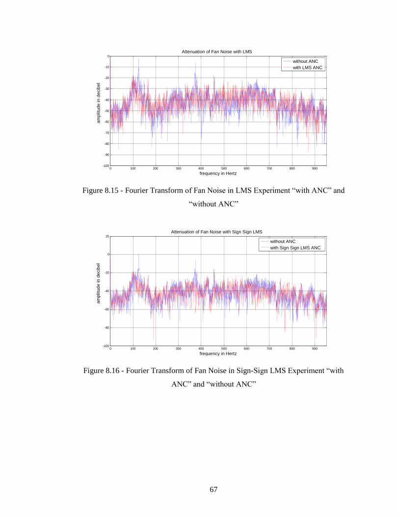
67
Figure 8.15 - Fourier Transform of Fan Noise in LMS Experiment “with ANC” and
“without ANC”
Figure 8.16 - Fourier Transform of Fan Noise in Sign-Sign LMS Experiment “with
ANC” and “without ANC”
0 100 200 300 400 500 600 700 800 900 -100
-90
-80
-70
-60
-50
-40
-30
-20
-10
0
frequency in Hertz
am
plit
ud
e in
decib
el
Attenuation of Fan Noise with LMS
without ANC with LMS ANC
0 100 200 300 400 500 600 700 800 900 -100
-80
-60
-40
-20
0
20
frequency in Hertz
am
plit
ud
e in
decib
el
Attenuation of Fan Noise with Sign Sign LMS
without ANC with Sign Sign LMS ANC

68
Figure 8.17 - Fourier Transform of Fan Noise in Analog ANC Headphone Experiment
“with ANC” and “without ANC”
Table 8.5 - The attenuation levels of fan noise
ANC system
frequency
Digital ANC
Headphone –
NLMS
Digital ANC
Headphone –
LMS
Digital ANC
Headphone –
Sign-Sign LMS
Analog
ANC
Headphone
125 Hz 21.3 dB 20.7 dB 22.4 dB 16.6 dB
374 Hz 19.3 dB 18.5 dB 18.3 dB 18.7 dB
The attenuation levels of the dominant frequency components are greater in
digital ANC headphone. On the other hand, the attenuation levels of analog ANC
headphone for weaker components smaller than 400 Hz is higher. Thus generally
speaking, the digital ANC system is good at reducing the dominant frequencies of this
wideband fan noise. The optimized filter coefficients in digital ANC try to decrease
power of error signal. The main components are attenuated whereas the audible weaker
components on the band are unaffected. On the other hand it can be seen that the
frequency band between 600Hz and 700Hz is attenuated about 5-10 dB by digital ANC
systems whereas the same frequency band is unaffected by analog ANC system.
0 100 200 300 400 500 600 700 800 900 -100
-90
-80
-70
-60
-50
-40
-30
-20
-10
0
frequency in Hertz
am
plit
ud
e in
decib
el
Attenuation of Fan Noise with Analog ANC Headphone
without ANC with Analog ANC Headphone

69
Actually digital ANC system attenuated even 850-900 Hz band whereas the analog ANC
system increases noises at these frequencies.
8.4 Propeller Cabin Noise Experiments
Figure 8.18, Figure 8.19, Figure 8.20 and Figure 8.21 show the results of the
experiments of LMS algorithm with propeller cabin noise whose main frequency
components are 83 Hz and 249 Hz. The attenuation level is calculated as 18.8 dB for 83
Hz and 19.3 dB for 249 Hz. In Figure 8.22, Figure 8.23 and Figure 8.24 the
corresponding results for normalized LMS, sign-sign LMS and analog ANC headphone
can be seen respectively. These results with the other systems experiment results are
listed in Table 8.6.
0 0.2 0.4 0.6 0.8 1 1.2 1.4 1.6 1.8 2
x 105
-0.06
-0.04
-0.02
0
0.02
0.04
0.06Propeller Cabin Noise - with Standard LMS
sample number
am
plit
ude -
linear
scale
Figure 8.18 - Propeller Cabin Noise in LMS Experiment “with ANC” and “without
ANC”

70
Figure 8.19 – Fourier Transform of Propeller Cabin Noise in LMS Experiment “without
ANC”
Figure 8.20 – Fourier Transform of Propeller Cabin Noise in LMS Experiment “with
ANC”
0 500 1000 1500 2000 2500 3000 3500 4000 0
0.2
0.4
0.6
0.8
1
1.2
1.4
1.6
1.8
X= 248.7751 Y= 0.11176
Fourier Transform of Propeller Cabin Noise - without ANC
frequency in Hertz
am
plit
ud
e -
line
ar
scale
50 100 150 200 250 300 350 400
-0.005
0
0.005
0.01
0.015
0.02
0.025
0.03
X= 82.3918 Y= 0.011579
Fourier Transform of Propeller Cabin Noise - with Standard LMS ANC
frequency in Hertz
am
plit
ud
e -
lin
ear
scale
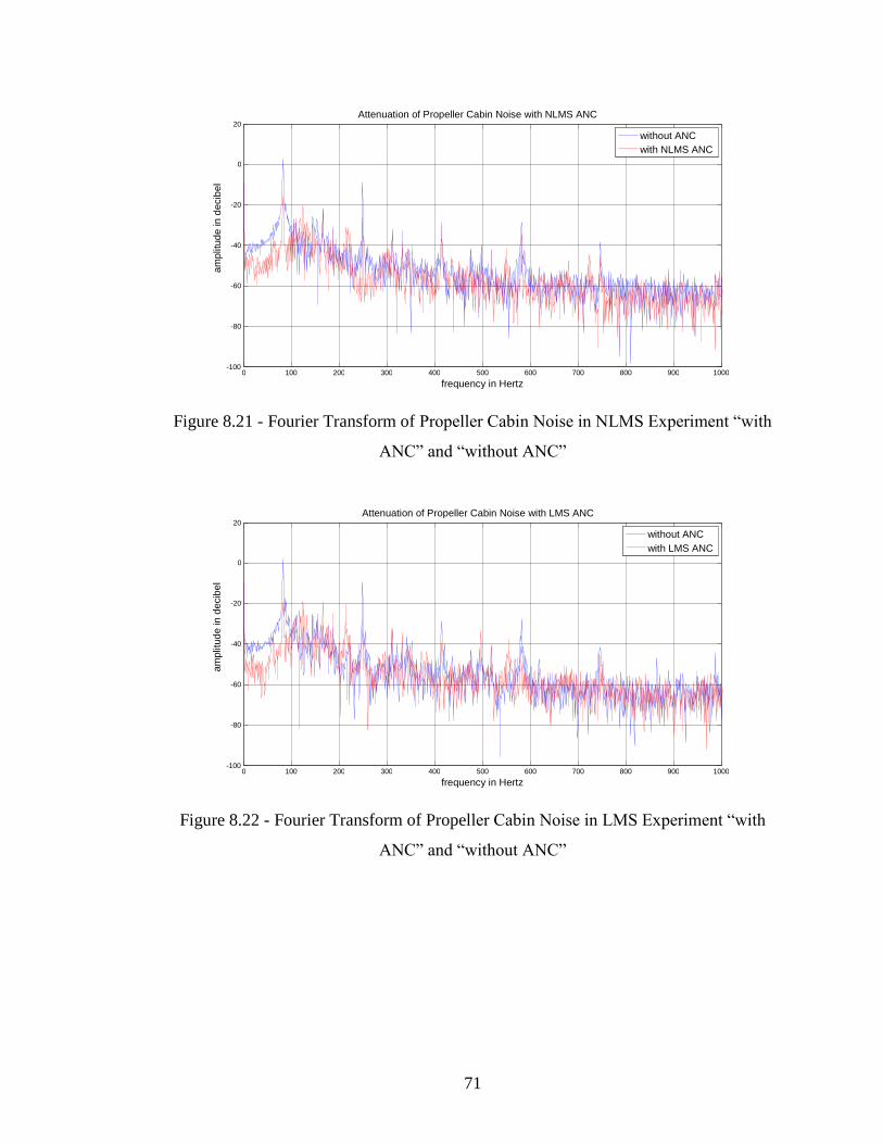
71
Figure 8.21 - Fourier Transform of Propeller Cabin Noise in NLMS Experiment “with
ANC” and “without ANC”
Figure 8.22 - Fourier Transform of Propeller Cabin Noise in LMS Experiment “with
ANC” and “without ANC”
0 100 200 300 400 500 600 700 800 900 1000 -100
-80
-60
-40
-20
0
20
frequency in Hertz
am
plit
ud
e in
decib
el
Attenuation of Propeller Cabin Noise with NLMS ANC
without ANC with NLMS ANC
0 100 200 300 400 500 600 700 800 900 1000 -100
-80
-60
-40
-20
0
20
frequency in Hertz
am
plit
ud
e in
decib
el
Attenuation of Propeller Cabin Noise with LMS ANC
without ANC with LMS ANC

72
Figure 8.23 - Fourier Transform of Propeller Cabin Noise in Sign-Sign LMS Experiment
“with ANC” and “without ANC”
Figure 8.24 - Fourier Transform of Propeller Cabin Noise in
Analog ANC Headphone Experiment “with ANC” and “without ANC”
0 100 200 300 400 500 600 700 800 900 1000 -100
-80
-60
-40
-20
0
20
frequency in Hertz
am
plit
ud
e in
decib
el
Attenuation of Propeller Cabin Noise with Sign Sign LMS ANC
without ANC with Sign Sign LMS ANC
0 100 200 300 400 500 600 700 800 900 1000 -100
-80
-60
-40
-20
0
20
frequency in Hertz
am
plit
ud
e in
decib
el
Attenuation of Propeller Cabin Noise with Analog ANC Headphone
without ANC with Analog ANC Headphone

73
Table 8.6 - The attenuation levels of propeller cabin noise
ANC system
frequency
Digital ANC
Headphone –
NLMS
Digital ANC
Headphone –
LMS
Digital ANC
Headphone –
Sign-Sign LMS
Analog
ANC
Headphone
83 Hz 18.8 dB 21.7 dB 21.2 dB 12.5 dB
249 Hz 19.3 dB 19.2 dB 16.7 dB 9.4 dB
The attenuation levels of dominant frequency components are higher in digital
system in propeller cabin noise experiment. However, analog system attenuates weaker
signals in the frequency band 50Hz – 300Hz. The digital system with optimized filter
coefficients mainly attenuates the dominant frequency components.
8.5 Drill Noise Experiments
Figure 8.25, Figure 8.26, Figure 8.27 and Figure 8.28 show the results of the
experiments of sign-sign LMS algorithm with drill noise whose main frequency
component is 450 Hz. The attenuation level is calculated as 10.8 dB for 450 Hz. In
Figure 8.29, Figure 8.30 and Figure 8.31 the corresponding results for NLMS, LMS and
analog ANC headphone can be seen respectively. These results with the other systems
experiment results are listed in Table 8.7.

74
0 0.5 1 1.5 2 2.5 3 3.5 4
x 105
-0.05
-0.04
-0.03
-0.02
-0.01
0
0.01
0.02
0.03
0.04
0.05Drill Noise with Sign Sign LMS
am
plit
ude -
linear
scale
sample number
Figure 8.25 - Drill Noise in Sign-Sign LMS Experiment “with ANC” and “without
ANC”
Figure 8.26 – Fourier Transform of Drill Noise in Sign-Sign LMS Experiment “without
ANC”
0 500 1000 1500 2000 2500 3000 3500 4000 0
0.02
0.04
0.06
0.08
0.1
0.12
0.14
X= 2274.9725 Y= 0.0018143
Fourier Transform of Drill Noise - without ANC
frequency in Hertz
am
plit
ud
e -
line
ar
scale

75
Figure 8.27 - Fourier Transform of Drill Noise in Sign-Sign LMS Experiment “with
ANC”
Figure 8.28 - Fourier Transform of Drill Noise in NLMS Experiment “with ANC” and
“without ANC”
400 600 800 1000 1200 1400 1600 1800 2000 2200
-2
0
2
4
6
8
10
12
x 10 -3
X= 2274.9725 Y= 0.0010143
frequency in Hertz
am
plit
ud
e -
line
ar
scale
Fourier Transform of Drill Noise - with Sign Sign LMS ANC
0 500 1000 1500 2000 2500 -90
-80
-70
-60
-50
-40
-30
-20
-10
0
frequency in Hertz
am
plit
ud
e in
decib
el
Attenuation of Drill Noise with NLMS ANC
without ANC with NLMS ANC
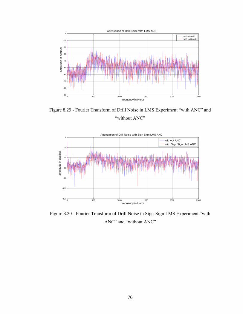
76
Figure 8.29 - Fourier Transform of Drill Noise in LMS Experiment “with ANC” and
“without ANC”
Figure 8.30 - Fourier Transform of Drill Noise in Sign-Sign LMS Experiment “with
ANC” and “without ANC”
0 500 1000 1500 2000 2500 -90
-80
-70
-60
-50
-40
-30
-20
-10
0
frequency in Hertz
am
plit
ud
e in
decib
el
Attenuation of Drill Noise with LMS ANC
without ANC with LMS ANC
0 500 1000 1500 2000 2500 -120
-100
-80
-60
-40
-20
0
frequency in Hertz
am
plit
ud
e in
decib
el
Attenuation of Drill Noise with Sign Sign LMS ANC
without ANC with Sign Sign LMS ANC

77
Figure 8.31 - Fourier Transform of Drill Noise in Analog ANC Headphone Experiment
“with ANC” and “without ANC”
Table 8.7 - The attenuation levels of drill noise
ANC system
frequency
Digital ANC
Headphone –
NLMS
Digital ANC
Headphone –
LMS
Digital ANC
Headphone –
Sign-Sign LMS
Analog
ANC
Headphone
450 Hz 10.8 dB 10.8 dB 10.7 dB 8.4 dB
910 Hz 4.0 dB 5.9 dB 5.4 dB -1.8 dB
1363 Hz 5.9 dB 2.1 dB 4.5 dB -2.4 dB
2275 Hz 4.7 dB 2.0 dB 2.5 dB *
*this high frequency component is cancelled mechanically by Analog ANC headphone.
The attenuation of dominant frequency component between 100Hz and 500Hz in
digital ANC system is higher in drill noise experiment. Attenuation levels of weaker
frequency components between 50-400Hz are higher in analog system. However, the
drill noise has higher frequency components especially distributed around 450 Hz, 900
Hz, 1300 Hz and 2250 Hz. Thus, analog ANC headphone is ineffective for this noise
type whereas digital ANC headphone continues attenuation. On the other hand, drill
noise is a very difficult noise type for digital adaptive ANC system because of its
wideband characteristics. Most of the frequency component of drill noise is unaffected.
0 500 1000 1500 2000 2500 -100
-90
-80
-70
-60
-50
-40
-30
-20
-10
0
frequency in Hertz
am
plit
ud
e in
decib
el
Attenuation of Drill Noise with Analog ANC Headphone
without ANC with Analog ANC Headphone

78
8.6 Tracking Capability Experiments
Tracking is the ability of the algorithm to track non-stationary signals. Figure
8.32, Figure 8.33, Figure 8.34 and Figure 8.35 show the results of each system under a
non-stationary sinusoidal signal.
0.5 1 1.5 2 2.5 3 3.5
x 105
-0.04
-0.03
-0.02
-0.01
0
0.01
0.02
0.03
NLMS Tracking Performance of Nonstationary Sinusoidal
am
plit
ude -
lin
ear
scale
sample number
without ANC
with NLMS ANC
Figure 8.32 – NLMS Tracking Performance with a Non-stationary Sinusoidal Signal
0.5 1 1.5 2 2.5 3 3.5
x 105
-0.04
-0.03
-0.02
-0.01
0
0.01
0.02
0.03
LMS Tracking Performance of Nonstationary Sinusoidal
am
plit
ude -
lin
ear
scale
sample number
without ANC
with LMS ANC
Figure 8.33 – LMS Tracking Performance with a Non-stationary Sinusoidal Signal

79
0.5 1 1.5 2 2.5 3 3.5
x 105
-0.04
-0.03
-0.02
-0.01
0
0.01
0.02
0.03
Sign Sign LMS Tracking Performance of Nonstationary Sinusoidal
am
plit
ude -
lin
ear
scale
sample number
without ANC
with Sign Sign NLMS
Figure 8.34 – Sign-Sign LMS Tracking Performance with a Non-stationary Sinusoidal
Signal
0.5 1 1.5 2 2.5 3 3.5
x 105
-0.03
-0.02
-0.01
0
0.01
0.02
Analog ANC Headphone Performance of Nonstationary Sinusoidal
am
plit
ude -
lin
ear
scale
sample number
without ANC
with Analog ANC headphone
Figure 8.35 – Analog ANC Headphone Performance with a Non-stationary Sinusoidal
Signal
The attenuation levels are better in digital ANC headphone than analog ANC
headphone as seen in above figures. Digital ANC system preserves attenuation even
though the primary noise levels are changed. This situation can be observed between the

80
samples 160000 and 250000. The responses of the system before the 50000th
sample
shows that the digital system tracks the decreasing slope of primary error signal. LMS
adaptation shows the best performance in tracking capability. Analog ANC headphone is
successful in the non-stationary signal experiment, because there is not a tracking
problem in fixed analog controllers.
8.7 Convergence Rate for Different LMS Algorithms
The following experiments are made to see the convergence rate for different
LMS algorithms. Figure 8.36, Figure 8.37 and Figure 8.38 are plotted in same scale
showing convergence rate for single tone of 300 Hz.
2.75 2.8 2.85 2.9 2.95 3 3.05
x 104
-0.3
-0.2
-0.1
0
0.1
0.2
0.3
Convergence of NLMS for Single Tone of 300 Hz
am
plit
ude -
lin
ear
scale
iteration number
Figure 8.36 – Convergence Rate of NLMS for Single Tone of 300 Hz

81
2.45 2.5 2.55 2.6 2.65 2.7 2.75 2.8
x 104
-0.2
-0.15
-0.1
-0.05
0
0.05
0.1
0.15
0.2
iteration number
am
plit
ude -
linear
scale
Convergence of LMS for Single Tone of 300 Hz
Figure 8.37 – Convergence Rate of LMS for Single Tone of 300 Hz
2.65 2.7 2.75 2.8 2.85 2.9 2.95
x 104
-0.3
-0.2
-0.1
0
0.1
0.2
0.3
Convergence of Sign Sign LMS for Single Tone of 300 Hz
am
plit
ude -
lin
ear
scale
iteration number
Figure 8.38 – Convergence Rate of Sign-Sign LMS for Single Tone of 300 Hz
As expected from theoretical discussions, NLMS has a faster convergence rate
than LMS and SSLMS has the slowest convergence rate.

82
8.8 Digital Residual Error Experiment
Three different primary noise levels are given to digital ANC headphone and the
attenuation amount in each step is observed. These three primary noise signals are
named as level-2, level-1 and level-0 with decreasing power. The minimum signal level
that can be attenuated by each algorithm is tried to be determined. The graphics are
drawn in the DSP debugger environment in real time.
The Fourier transform of a primary noise signal of level-2 400 Hz is given in
Figure 8.39. The residual error levels are seen for NLMS, LMS and SSLMS algorithms
respectively in Figure 8.40, Figure 8.41 and Figure 8.42. Similarly a weaker 400 Hz
signal (marked as level-1 amplitude) seen in Figure 8.43 is applied to the systems and
the responses in Figure 8.44, Figure 8.45 and Figure 8.46 are recorded. The last group of
figures from Figure 8.47 to Figure 8.50 shows the results for the weakest primary test
signal (marked as level-0 amplitude) for which the algorithms are on the edge of
stopping or severely slowing down.
Figure 8.39 – Primary Noise for LMS Experiments for level-2 400 Hz signal
amplitude –linear scale
frequency = x*8000Hz

83
Figure 8.40 – Residual Error for NLMS Experiment for level-2 400 Hz signal
Figure 8.41 – Residual Error for LMS Experiment for level-2 400 Hz signal
amplitude –linear scale
frequency = x*8000Hz
amplitude –linear scale
frequency = x*8000Hz

84
Figure 8.42 – Residual Error for Sign-Sign LMS Experiment for level-2 400 Hz signal
Figure 8.43 – Primary Noise for LMS Experiments for level-1 400 Hz signal
amplitude –linear scale
frequency = x*8000Hz
amplitude –linear scale
frequency = x*8000Hz

85
Figure 8.44 – Residual Error for NLMS Experiment for level-1 400 Hz signal
Figure 8.45 – Residual Error for LMS Experiment for level-1 400 Hz signal
amplitude –linear scale
frequency = x*8000Hz
amplitude –linear scale
frequency = x*8000Hz

86
Figure 8.46 – Residual Error for Sign-Sign LMS Experiment for level-1 400 Hz signal
Figure 8.47 – Primary Noise for LMS Experiments for level-0 400 Hz signal
amplitude –linear scale
frequency = x*8000Hz
amplitude –linear scale
frequency = x*8000Hz

87
Figure 8.48 – Residual Error for NLMS Experiment for level-0 400 Hz signal
Figure 8.49 – Residual Error for LMS Experiment for level-0 400 Hz signal
amplitude –linear scale
frequency = x*8000Hz
amplitude –linear scale
frequency = x*8000Hz

88
Figure 8.50 – Residual Error for Sign-Sign LMS Experiment for level-0 400 Hz signal
The results of these experiments showed that the digital residual error values are
different for different adaptation algorithms. However, it is obvious that the attenuation
levels are decreasing with decreasing primary noise levels in every algorithm. Moreover,
below a determined primary noise level the adaptation ceases. It is seen that NLMS and
SSLMS continues to attenuate even level-0 primary noise level, nevertheless LMS stops
adapting at this level. It is experimentally seen that the slowdown phenomenon can be
seen in fixed point environment when the primary noise signal is too low.
8.9 Drill Noise Experiment: Sub-band Filtering
How can the wideband drill noise be attenuated by digital system not only for its
dominant frequencies but also for the other harmonics? To answer this question drill
noise is filtered by a band pass filter whose pass band is 400 Hz - 500 Hz. The fourier
transform of NLMS for drill noise around 400-500 Hz is given in Figure 8.51. The
fourier transform of NLMS algorithm for band pass filtered drill noise is given in Figure
amplitude –linear scale
frequency = x*8000Hz

89
8.52. The attenuation of dominant frequency component at 450 Hz is 3 dB more than the
attenuation in previous experiment. Moreover, some weaker harmonics around these
dominant frequencies are attenuated only in this experiment. It is shown that total power
attenuation is improved when the signal is made band limited. According to [25] sub-
band filtering enhances the attenuation because of the decrease in eigenspread of each
band limited primary noise piece. This result may be extended to dividing the signal in
several bands around dominant frequencies and introducing individual adaptive filters
for each band working in parallel.
Figure 8.57 – The Attenuation of Normal Drill Noise by NLMS
Figure 8.58 – The Attenuation of Bandpass Filtered Drill Noise by NLMS
400 410 420 430 440 450 460 470 480 490 500 -80
-70
-60
-50
-40
-30
-20
-10
frequency in Hertz
am
plit
ud
e in
decib
el
NLMS Attenuation Results of Drill Noise
without ANC with NLMS ANC
400 410 420 430 440 450 460 470 480 490 500 -70
-60
-50
-40
-30
-20
-10
0
frequency in Hertz
am
plit
ud
e in
decib
el
NLMS Attenuation Results of Drill Noise after it is passed through a bandpass of 400-500Hz
without ANC with NLMS ANC

90
8.10 Discussion of the Test Results of Digital ANC Headphone System
The digital system attenuation is about 25dB for single tones of 100Hz to 400
Hz. The attenuation levels are decreased for frequencies higher than 800 Hz down to 15
dB. The attenuation amount of each frequency component in a multi tone signal
decreases as the dominance of this component in the overall signal decreases.
It is shown that NLMS is superior to other LMS algorithms in terms of
convergence. The general attenuation levels of single tones are highest for LMS.
SSLMS suffers from its slower convergence rate.
Digital systems are less effective than analog systems if the noise is distributed
widely between 50Hz and 400 Hz, because the power reduction optimization of the
adaptation algorithm causes the attenuation to be concentrated on dominant tones.
Moreover, wideband noise is difficult to be attenuated by using only one adaptive filter.
These insufficient attenuation levels of digital systems for wideband noises can be
improved by a more qualitative filtering method: sub-band filtering.
DRE is inversely proportional to primary noise signal levels. Thus decreasing
primary noise signals cause the adaptation process to terminate prematurely or continue
with very small correction terms, i.e. the adaptation enters slowdown region.
The Bose Analog ANC Headphone is successful especially for wideband noises
having frequency components lower than 300 Hz. However, it is insufficient for
frequencies greater than 400 Hz. Moreover, analog ANC headphone starts to increase
noises of frequencies greater than 700Hz - 800Hz. Its performance for very fast
changing signals whose dominant frequency component is around 50Hz – 200Hz is
superior to digital ANC headphone. On the other hand, it is obvious that slow changing
signals within frequencies of around 300 – 800 Hz is tracked and more successfully
attenuated by the digital ANC headphone system than the analog ANC headphone.

91
Another result is that successful mounting of analog ANC system on head
contributes in noise cancellation. However, it should be noted that the mechanical
attenuation is effective for frequencies higher than 400 Hz. It is experimentally seen in
digital ANC system that the attenuation levels are increased when the headphone is tried
to be tightly mounted on head. This action also increases the dynamic range as a result
of the decrease in the error input to the microphone. As a result it can be said that a
tighter mounting headphone should be selected for digital ANC system.

92
CHAPTER 9
CONCLUSION
In this thesis, the design and implementation of a portable fixed point digital
ANC headphone system is achieved. The theoretical results of fixed point LMS are
applied to real time ANC implementation.
LMS, normalized LMS and sign-sign LMS algorithms were studied. These
algorithms were implemented as filtered input type. The problem of slowdown
phenomenon in fixed point implementation has been examined. Step size selection in
fixed point environment has been made. The delays inherent to digital systems and their
importance in synchronization of the LMS adaptation algorithm were stated and
necessary modifications are applied. A compact, noise immune and convenient card
based on TMS320VC5416 Fixed point DSP was designed and produced. The card was
designed such that further improvements or modifications can be done easily on
hardware.
The performance of the digital device was compared with an analog ANC
headphone with artificial signals as well as with natural signals. The tracking capability
of the digital system was tested. Convergence rate of different LMS adaptation
algorithms were compared. The digital residual error resulted from slowdown
phenomenon was experimentally seen. Additionally, software adjustments for the
practical usage of the digital system were introduced to prevent divergence of the system
when the headphone is put off. The basis of further improvements in attenuation for
digital ANC system was stated as sub-band filtering.
It is seen that the digital system is capable of attenuating frequencies from 80 Hz
up to 1000 Hz especially when the noise is narrowband. The attenuation level is about
93
25 dB for narrow band signals between 80 Hz and 400 Hz. For higher frequencies up to
1000 Hz this attenuation level is about 15 dB.
Fixed analog controller in this study has a predefined optimum attenuation band.
This optimum band is between 50 Hz and 400 Hz. The analog system is ineffective for
frequencies higher than 400 Hz. Moreover, it increases frequency components higher
than 700-800Hz. The attenuation levels of digital ANC system are much higher than the
attenuation levels of analog system when the noise is narrowband. On the other hand,
the attenuation level of digital ANC system is lower than analog ANC system for
weaker frequency components when the noise is wideband, because filter coefficients
are optimized to decrease the power of residual error and dominant frequency
components are more effective on power of this error signal. One adaptation filter is
insufficient when the noise is spread equally over a wide frequency band. It is
experimentally seen that the adaptation of digital system can be improved for wideband
noises by dividing the noise in sub-bands and applying individual filters for each
partition.
It is seen that the digital system is affected by delays existing between analog
and digital parts of headphone system. Digital residual error originating from fixed point
implementation affects low level signal attenuation.
Normalized LMS algorithm is superior to other adaptation algorithms for its
small digital residual error and high convergence rate. However, NLMS has a drawback
for its inherent arithmetic complexity in fixed point implementation. Sign-sign LMS
algorithm has the slowest convergence rate.
Unfortunately, the dynamic range of the designed digital system is not as good as
analog ANC system. When the upper limit for primary noise signal is increased by
decreasing step size the system becomes less sensitive to lower amplitude noise signals
due to slowdown phenomenon whereas a larger step size increases results in divergence
for high level primary noise signals. This problem can not be solved by increasing the

94
resolution because of increasing computational complexity. An educated step size
sequence should be implemented such that the high level noises do not cause the system
to diverge and low level noises do not create high digital residual error.
The mechanical design of the headphone was seen to be very critical to increase
noise attenuation. Moreover, the tight mounting of the headphone resulted in the
increase in dynamic range.
In conclusion, it is shown that adaptive ANC headphone system can be
implemented digitally by using a fixed point processor. The attenuation levels can be
increased by adaptive digital systems at about 10 dB compared with analog ANC
systems when the noise is narrowband. Moreover, noise signals having frequency
components higher than 400 Hz is attenuated in digital systems contrary to analog
systems.
9.1 Future Work
The effectiveness of digital system should be extended to wider band noises by
some additional improvements. It is seen that this improvement can be supplied by sub-
band filtering which is achievable in the designed card of this study by an FPGA. FPGA
is a suitable environment for such parallel synchronous operations. Actually a
combination of DSP and FPGA controller can be used for optimized processing
performance [26].
The mechanical design of digital ANC headphone should be improved. The tight
mounting of headphone and mechanical attenuation is shown to be very important as a
contribution to the overall attenuation.
The increase in clock rates of DSP and the resolution of CODECs results in
much more computational capacity and decrease in the least significant digit values.

95
This makes fixed point limitations become less effective as the results of extended
resolution, signal to noise ratio and total harmonic distortion.
An adaptive step size selection sequence increases the dynamic range of fixed
point implemented LMS.

96
REFERENCES
[1] C.M. Harris, Handbook of Acoustical measurements and Noise Control, 3rd
ed.
New York: McGraw-Hill, 1991
[2] P. Lueg “Process of silencing sound oscillations” U.S. Patent 2,043,416 June 9,
1936
[3] H. F. Olson and E. G. May, “Electronic sound absorber,” Acoust. Soc. Amer. vol.
25, pp. 1130–1136, Nov. 1953.
[4] Sen M. Kuo and Dennis R. Morgan “Active Noise Control: A Tutorial Review” in
Proceedings of the IEEE, vol. 87, no. 6 June 1999.
[5] Dorey, A.P., S.F. Pelc, R.D. Rawlinson and P.D Wheeler. “The Development
and Testing of an Active Noise Reduction System For use in Ear Defenders,”
Proc. Inter-Noise 78. pp. 977-982, 1978.
[6] Simon Haykin, “Adaptive Filter Theory”, Prentice Hall, 1996.
[7] Simon Haykin, “Adaptive Filters”, Signal Processing Magazine, IEEE Computer
Society, 1999.
[8] Woon S. Gan, Sohini Mitra and Sen M. Kuo, “Adaptive Feedback Active Noise
Control Headset: Implementation, Evaluation and Its Extensions” IEEE
Transactions on Consumer Electronics, Vol. 51, No.3, August 2005.
[9] Sen M. Kuo, Sohini Mitra and Woon-Seng Gan, “Adaptive Feedback Active
Noise Control Headset: Implementation, Evaluation and Its Extensions” IEEE
Transactions on Control Systems Technology , Vol. 14, No.2, March 2006.
[10] D. R. Morgan, “An analysis of multiple correlation cancellation loops with a
filter in the auxiliary path,” IEEE Trans. Acoust., Speech, Signal Processing, vol.
ASSP-28, pp. 454–467, Aug. 1980.
[11] S. J. Elliott and P. A. Nelson, “Active noise control,” IEEE Signal Processing
Mag., Vol. 10, pp. 12–35, Oct. 1993.

97
[12] Richard D. Gitlin, J. E. Mazo and Michael G. Taylor, “On the design of Gradient
Algorithms for Digitally Implemented Adaptive Filters”, IEEE Transactions On
Circuit Theory, Vol. ct-20, No.2, March 1973.
[13] Christos Caraiscos and Bede Liu, “A Roundoff Error Analysis of the LMS
Adaptive Algortihm”, IEEE Transactions on Acoustics, Speech and Signal
Processing, Vol. ASSP-32, No.1, February 1984.
[14] Neil J. Bershad, and Jose Carlos M. Bermudez, “New Insights on the Transient
and Steady-State Behaviour of the Quantized LMS Algorithm”, IEEE
Transactions on Signal Processing, Vol. 44, No.10, October 1996.
[15] Riten Gupta and Alfred O.Hero, “Power versus Performance Tradeoffs for
Reduced Resolution LMS Adaptive Filters”, IEEE Transactions on Signal
Processing, Vol. 48, No.10, October 2000.
[16] Neil J. Bershad, and Jose Carlos M. Bermudez, “A Nonlinear Analytical Model
for the Quantized LMS Algorithm – The Power-of-Two Step Size Case”, IEEE
Transactions on Signal Processing, Vol. 44, No.11, November 1996.
[17] Neil J. Bershad, and Jose Carlos M. Bermudez, “A Nonlinear Analytical Model
for the Quantized LMS Algorithm – Arbitrary Step Size Case”, IEEE
Transactions on Signal Processing, Vol. 44, No.5, May 1996.
[18] Nabil R. Yousef and Ali H. Sayed, “Fixed Point Steady-State Analysis of
Adaptive Filters”, International Journal of Adaptive Control and Signal
Processing, Vol. 17, pp. 237-258, March 2003.
[19] Sen M. Kuo and Dennis R. Morgan, “Active Noise Control Systems: Algorithms
and DSP Implementations”, John Wiley & Sons Inc., New York, 1996.
[20] Texas Instruments, “TMS320VC5416 Fixed-Point Digital Signal Processor Data
Manual”, Literature Number: SPRS095O, January 2005.
[21] Texas Instruments, “TMS320C54x DSP Reference Set Volume 1: CPU and
Peripherals” Literature Number: SPRU131F, April 1999.
[22] Texas Instruments, “TMS320C54x DSP Library Programmer’s Reference”
Literature Number: SPRU518C, August 2002.
[23] Texas Instruments, “TLV320AIC20K Codec Data Manual” Literature Number:
SLAS363D, April 2005.
[24] Texas Instruments “TMS320C54x Chip Support Library API Reference Guide”
Literature Number: SPRU420E, July 2003.

98
[25] Victor DeBrunner, Linda S. DeBrunner and Longji Wang, “Sub-band Adaptive
Filtering With Delay Compensation for Active Control”, IEEE Transactions on
Signal Processing, Vol. 52, No.10, October 2004.
[26] Reza Hashemian, “Design of an Active Noise Control System Using
Combinations of DSP and FPGAs”, PLD Conference Proceedings, 1995.
[27] Knowles Acoustics, SP0103NC Specification Document.
[28] Markus Rupp and Ali H. Sayed “Robust FxLMS Algorithms with Improved
Convergence Performance”, IEEE Transactions on Speech and Audio
Processing, Vol. 6, No. 1, January 1998

99
APPENDIX A
HARDWARE DESIGN OF DIGITAL ANC HEADPHONE
SYSTEM
Basic serial port connections between TLV320AIC20K CODEC and
TMS320VC5416 CODEC can be seen in Figure A.1.
Figure A.1 – Serial Port Connections between TLV320AIC20K and DSP
An AMD29LV160DT-90EI flash-ROM is placed on card for the DSP to run
independent of the emulator connection. The program is coded to the flash-ROM
through emulator once and on each power-up the code is copied to the DSP. DSP starts
to run from the starting point of this code.

100
Additionally, a Field Programmable Gate Array (Xilinx XC3S1000 FPGA)
within a PROM (the code of RAM based FPGA resides on PROM) is placed on board
for flexibility to develop other algorithms. Alternative paths from CODECs to the FPGA
are supplied. There exists a parallel address/data bus between DSP and FPGA. The
reason for this improvement is for possible future work. The advantages of FPGA based
implementation considering some real implementation issue is explained in Chapter 9.
A second CODEC is placed on the card for some possible additional connections
such as line-in.
The power management of the card is based on four MAXIM MAX1793
regulators which produce 3.3V, 1.8V, 1.5V and 1.2V for different components on the
board. These regulators can work with voltages up to 5.5V as input.
The reset management is accomplished by MAX6707TKA-T reset supervisor.
This component resets the intelligent devices on board when there exists a certain
decrease in voltages 3.3V and 1.5V. The CODEC is reset through a general purpose
output of the DSP by software.
The clock is supplied by an EC54 SMX7 24MHz clock oscillator and it passes
through a Linear Technology LT1719IS6 operational amplifier for a clear square wave
of 24 MHz. This clock is fed to the DSP and FPGA as the main clock sources. Inside the
DSP, this rate is increased to 120MHz by the PLL. The 30MHz output clock of the DSP
is given to the CODEC as its main clock. The 256 KHz clock and 8 KHz
synchronization signal for the serial data and command interface between DSP and
CODEC are supplied by the CODEC.
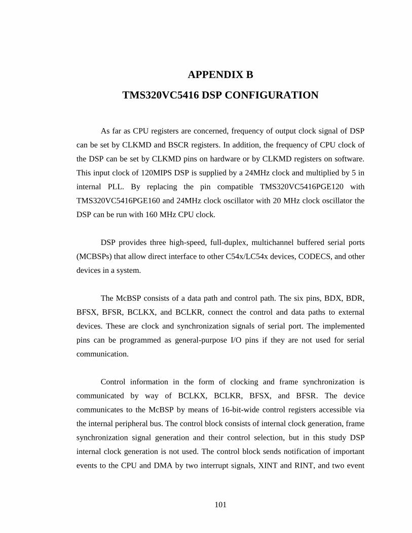
101
APPENDIX B
TMS320VC5416 DSP CONFIGURATION
As far as CPU registers are concerned, frequency of output clock signal of DSP
can be set by CLKMD and BSCR registers. In addition, the frequency of CPU clock of
the DSP can be set by CLKMD pins on hardware or by CLKMD registers on software.
This input clock of 120MIPS DSP is supplied by a 24MHz clock and multiplied by 5 in
internal PLL. By replacing the pin compatible TMS320VC5416PGE120 with
TMS320VC5416PGE160 and 24MHz clock oscillator with 20 MHz clock oscillator the
DSP can be run with 160 MHz CPU clock.
DSP provides three high-speed, full-duplex, multichannel buffered serial ports
(MCBSPs) that allow direct interface to other C54x/LC54x devices, CODECS, and other
devices in a system.
The McBSP consists of a data path and control path. The six pins, BDX, BDR,
BFSX, BFSR, BCLKX, and BCLKR, connect the control and data paths to external
devices. These are clock and synchronization signals of serial port. The implemented
pins can be programmed as general-purpose I/O pins if they are not used for serial
communication.
Control information in the form of clocking and frame synchronization is
communicated by way of BCLKX, BCLKR, BFSX, and BFSR. The device
communicates to the McBSP by means of 16-bit-wide control registers accessible via
the internal peripheral bus. The control block consists of internal clock generation, frame
synchronization signal generation and their control selection, but in this study DSP
internal clock generation is not used. The control block sends notification of important
events to the CPU and DMA by two interrupt signals, XINT and RINT, and two event

102
signals, XEVT and REVT. The interior block diagram of McBSP is given in Figure B.1.
In this study DMA is not used, CPU directly interfaces with McBSP.
The CPU or the DMA controller reads the received data from the data receive
register (DRR[1,2]) and writes the data to be transmitted to the data transmit register
(DXR[1,2]). Data written to DXR[1,2] is shifted out to DX via the transmit shift register
(XSR[1,2]). Similarly, receive data on the DR pin is shifted into the receive shift register
(RSR[1,2]) and copied into the receive buffer register (RBR[1,2]). RBR[1,2] is then
copied to DRR[1,2], which can be read by the CPU or the DMA controller. This allows
simultaneous movement of internal and external data communications. DRR2, RBR2,
RSR2, DXR2, and XSR2 registers are not utilized (written, read, or shifted) if the
receive/transmit word length, R/XWDLEN[1,2], is specified for 8-, 12-, or 16-bit mode.
The control registers for the multichannel buffered serial port are accessed using
the subbank addressing scheme. This allows a set or subbank of registers to be accessed
through a single memory location. The McBSP subbank address register (SPSA) is used
as a pointer to select a particular register within the subbank. The McBSP data register
(SPSDx) is used to access (read or write) the selected register. Alternatively, one can
benefit from chip support library to use predefined functions for register assignments.
The McBSP registers and their corresponding values specific to this study are as
follows: SPCR1 register is set as the digital loopback mode disabled, receive interrupt is
dedicated to RRDY signal and reset is applied to receive port. SPCR2 register is set to
disable internal sample rate generator of TMS320VC5416, transmit interrupt is
dedicated to XRDY signal and reset is applied to transmit port. The RCR and XCR
registers are set as single-phase frames of 4 words consisting of 16 bits. Lastly, Pin
Control Register is set as frame synchronization and clock signals are input. Frame
synchronization signals are active high signals. PCR register configuration also dictates
that the transmit clock, samples data at rising edges whereas the receive clock, samples
data at falling edges.

103
Figure B.1 – Block Diagram of Multichannel Buffered Serial Port in TMS320VC5416
DSP

104
APPENDIX C
TLV320AIC20K CODEC CONFIGURATION
TLV320AIC20K has several types of inputs and outputs for various load and
source types such as Microphone / 8 Ohm Speaker, 600 Ohm Line In/ Line Out, 150
Ohm Headset In/ Headset Out, 150 Ohm Handset In / Handset Out. The block diagram
of one channel of CODEC is in Figure C.1. Actually there exists another channel in
TLV320AIC20K with same block diagram.
Figure C.1 – The Block Diagram of One Channel of TLV320AIC20K CODEC
The configuration of the codec defines the following parameters which are critical:
The data rate of the serial port communication
The sampling frequency of the ADC and DAC
The input/output connections
The amplifier gain for input/output
The voltage level for Microphone Bias Output

105
Interpolation / Decimation Filter disabling
Each channel in TLV320AIC20K contains 6 control registers that are used to
program available modes of operation. All register programming is achieved by the
control frame through DIN. New configuration takes effect after a delay of one frame
synchronization signal. The serial interface is defaulted to programming mode upon
power-up. 6th bit of Control Register-1 is set for continuous data transfer mode. The
form of the registers to be written is in Table C.1 and crucial settings are given in Table
C.2.
The configuration of TLV320AIC20K CODEC is made by TMS320VC5416
DSP through McBSP0 serial port which is also used for data communication. During
configuration, as mentioned in DSP configuration, each frame consists of 4 words. The
first and third words in this frame carry the configuration word for first and second
channel of CODEC respectively. The second and fourth words carry corresponding data
samples. Upon completion of the configuration, the serial port of DSP is reconfigured to
carry 2 words in each frame which consists of only data samples.
Table C.1 – TLV320AIC20K CODEC Write Register Form
D15-D13 Control Register Address
D12 (0) write – (1) read
D11 broadcast (1)
D7 – D0 Register Content

106
Table C.2 - TLV320AIC20K CODEC Register Content
Register-1 00101001 The bias voltage of SP0103NC microphone is
set to 2.35V.
Register-2 11100000 Decimation/Interpolation Filters are disabled
Register-3A 00011001 No power-down is chosen for the device to
operate in normal mode.
Register-3B 01000000 Bandpass filter is disabled.
Register-3C 10000000 -
Register-3D 11000000 -
Register-4 11110101 and
00001010
Frame Synchronization signal is set to 8KHz
by FS = MCLK / MNP
SCLK is 32xFS for continuous data transfer
mode and 64xFS for programming mode
Register-5A 00010100 ADC gain is set to 42 dB
Register-5B “01010100 DAC gain is set to -13.5 dB
Register-5C 10000000 -
Register-5D 11000000 -
Register-6A 00000001 Headset Input for CH1 /
Handset Input for CH2
Register-6B 00000002 Headset Output for CH1 /
Handset Output for CH2


