8/2/2019 A Simulation-Based Performance Comparison of the Minimum Node Size and Stability-Based Connected Dominating…
http://slidepdf.com/reader/full/a-simulation-based-performance-comparison-of-the-minimum-node-size-and-stability-based 1/16
International Journal of Computer Networks & Communications (IJCNC) Vol.4, No.2, March 2012
DOI : 10.5121/ijcnc.2012.4211 169
A SIMULATION-BASED PERFORMANCE
COMPARISON OF THE MINIMUM NODE SIZE AND
S TABILITY -BASED CONNECTED DOMINATING
SETS FOR MOBILE A D HOC NETWORKS
Natarajan Meghanathan
Jackson State University, Jackson, MS, USAE-mail: [email protected]
A BSTRACT
The high-level contribution of this paper is a simulation-based comparison of two contrasting categories
(minimum node size vs. stability) of connected dominating sets for mobile ad hoc networks. We pick the
maximum density-based CDS (MaxD-CDS) and Node ID-based CDS (ID-CDS) to be representatives of the minimum node size-based CDS algorithms; the minimum velocity-based CDS (MinV-CDS) and the
node stability index-based CDS (NSI-CDS) are chosen as representatives for stability-driven CDS. The
MaxD-CDS, ID-CDS and MinV-CDS algorithms prefer to respectively include nodes with a larger
number of uncovered neighbors, larger node ID and lower velocity into the CDS; the NSI-CDS algorithm
prefers to include nodes with a larger value for the sum of the predicted expiration times of the links with
the neighbor nodes. We simulate these algorithms under diverse conditions of node mobility and network
density. We observe the MinV-CDS to be the most stable among all the CDSs as well as incur a lower hop
count per path (through the CDS nodes) between any two nodes in the network. However, the MinV-CDS
incurs a relatively larger CDS node size and edge size compared to the other three CDSs. Owing to a
larger control overhead that could be incurred while broadcasting through a MinV-CDS (with larger
number of CDS nodes and edges), the NSI-CDS can be considered as the best choice from the points of
view of delay, energy, bandwidth and fairness of node usage.
K EYWORDS Connected Dominating Sets, CDS Lifetime, CDS Node Size, Tradeoff, CDS Algorithms, Mobile Ad hoc
Networks, Simulations
1. INTRODUCTION
A Mobile ad hoc network (MANET) is a category of wireless networks in which the topology
changes dynamically with time due to arbitrary node movement. The MANET nodes have
limited battery charge and hence operate with a restricted transmission range to conserve energyas well as avoid interference and collisions that may result from transmitting over longer
distances. As a result, MANET routes are often multi-hop in nature and also temporally changedepending on node mobility and availability. MANET routing protocols (for unicasting,
multicasting and broadcasting) have been predominantly designed to be on-demand in nature
rather than using a proactive strategy of determining the routes irrespective of the need [1][2].
The MANET on-demand routing protocols typically use a network-wide broadcast route-replycycle (called flooding) to discover the appropriate communication topology (path, tree or mesh)
[3]. A source node initiates the flooding of the Route-Request (RREQ) packets that propagatethrough several paths and reach the targeted destination (for unicasting) or receiver nodes (for
multicasting). These nodes choose the path that best satisfies the principles of the routingprotocol in use and respond with a Route-Reply (RREP) packet to the source on the selected
8/2/2019 A Simulation-Based Performance Comparison of the Minimum Node Size and Stability-Based Connected Dominating…
http://slidepdf.com/reader/full/a-simulation-based-performance-comparison-of-the-minimum-node-size-and-stability-based 2/16
International Journal of Computer Networks & Communications (IJCNC) Vol.4, No.2, March 2012
170
route. With flooding, every node in the network is required to broadcast the RREQ packet
exactly once in its neighborhood. Nevertheless, the redundancy of retransmissions and theresulting control overhead incurred with flooding is still too high, as every node spends energy
and bandwidth to receive the RREQ packet from each of its neighbors.
A Connected Dominating Set (CDS) of a network graph comprises of a subset of the nodes such
that every node in the network is either in the CDS or is a neighbor of a node in the CDS.Recent studies (e.g. [4][5][6][7][8]) have shown the CDS to be a viable backbone for network-
wide broadcasting of a message (such as the RREQ message), initiated from one node. Themessage is broadcast only by the CDS nodes (nodes constituting the CDS) and the non-CDS
nodes (who are neighbors of the CDS nodes) merely receive the message, once from each of their neighboring CDS nodes. The efficiency of broadcasting depends on the CDS Node Size
that directly influences the number of redundant retransmissions. One category of CDSalgorithms for MANETs aim to determine CDSs with reduced Node Size (i.e., constituent
nodes) such that whole network could be covered as fewer nodes as possible. However, asobserved in this paper and some of our previous work [9], such minimum node size-driven CDS
have been observed to be unstable (i.e. have a limited lifetime). The other category of MANET
CDS algorithms focus on maximizing the CDS Lifetime such that the control overhead incurred
in frequently reconfiguring a CDS is reduced. Such stability-driven CDSs have been observed[9] to incur a larger Node Size and ratified through the simulation studies in this paper. We
evaluate the tradeoff by calculating the ratio of the Node Size and Lifetime for the two
categories of CDS algorithms.
We pick the maximum density-based CDS (MaxD-CDS) [10] and Node ID-based CDS (ID-CDS) [11] to be representatives of the minimum node size-based CDS algorithms; the minimum
velocity-based CDS (MinV-CDS) [12] and the node stability index-based CDS (NSI-CDS) [9]are chosen as representatives for stability-driven CDS. The NSI of a node is defined as the sum
of the predicted expiration times of the links (LETs) with the neighbor nodes that are not yet
covered by a CDS node; the NSI-CDS algorithm prefers to include nodes with larger NSI valuesinto the CDS. The MaxD-CDS algorithm prefers to include nodes with the largest number of uncovered neighbors into the CDS; the ID-CDS algorithm prefers to include nodes with a larger
node ID and having at least one uncovered neighbor into the CDS; and the MinV-CDS
algorithm opts for slow moving nodes to be part of the CDS. We evaluate the four CDSalgorithms under diverse conditions of network density and node mobility with respect to four
metrics: CDS Lifetime, CDS Node Size, CDS Edge Size and the Hop Count per Path. To thebest of our knowledge, we could not find such a comprehensive comparison study of the
different CDS algorithms in the MANET literature.
We observe the MinV-CDS to incur a significantly larger lifetime compared to the other threeCDSs as well as incur a lower hop count per path (through the CDS nodes) between any two
nodes in the network. However, the MinV-CDS requires relatively more nodes to be part of theCDS to provide stability. Nevertheless, the Node Size-Lifetime tradeoff ratio is observed to be
the lowest for the MinV-CDS for a majority of the scenarios. The rest of the paper is organized
as follows: Section 2 presents a generic CDS algorithm that can be used to study each of the
four CDS algorithms (MaxD-CDS, ID-CDS, MinV-CDS and NSI-CDS) that will be analyzed in
the simulations. Section 3 presents the algorithm used to validate the existence of a currentlyknown CDS at a particular time instant and decide on the need to determine a new CDS. Section
4 presents examples to illustrate the construction of the two minimum node size-based CDS(ID-CDS and MaxD-CDS). Section 5 presents examples to illustrate the construction of the two
stability-based CDS (MinV-CDS and NSI-CDS). Section 6 presents the simulation resultsobserved for these four CDSs and evaluates the Node Size – Lifetime tradeoff. Section 7
concludes the paper and describes future work. Throughout the paper, the terms ‘vertex’ and‘node’, ‘edge’ and ‘link’, ‘path’ and ‘route’, ‘packet’ and ‘message’ are used interchangeably.
They mean the same.
8/2/2019 A Simulation-Based Performance Comparison of the Minimum Node Size and Stability-Based Connected Dominating…
http://slidepdf.com/reader/full/a-simulation-based-performance-comparison-of-the-minimum-node-size-and-stability-based 3/16
International Journal of Computer Networks & Communications (IJCNC) Vol.4, No.2, March 2012
171
2. GENERIC CDS CONSTRUCTION ALGORITHM
In this section, we present a generic algorithm that can be used to construct the four different
CDSs, with appropriate changes in the data structure (Priority-Queue) used to store the list of covered nodes that could be the candidate CDS nodes and the use of the appropriate criteria in
each of the iterations of the algorithm to evolve the particular CDS of interest. The advantage
with proposing a generic algorithm is that all the four CDSs can be constructed with virtuallythe same time complexity.
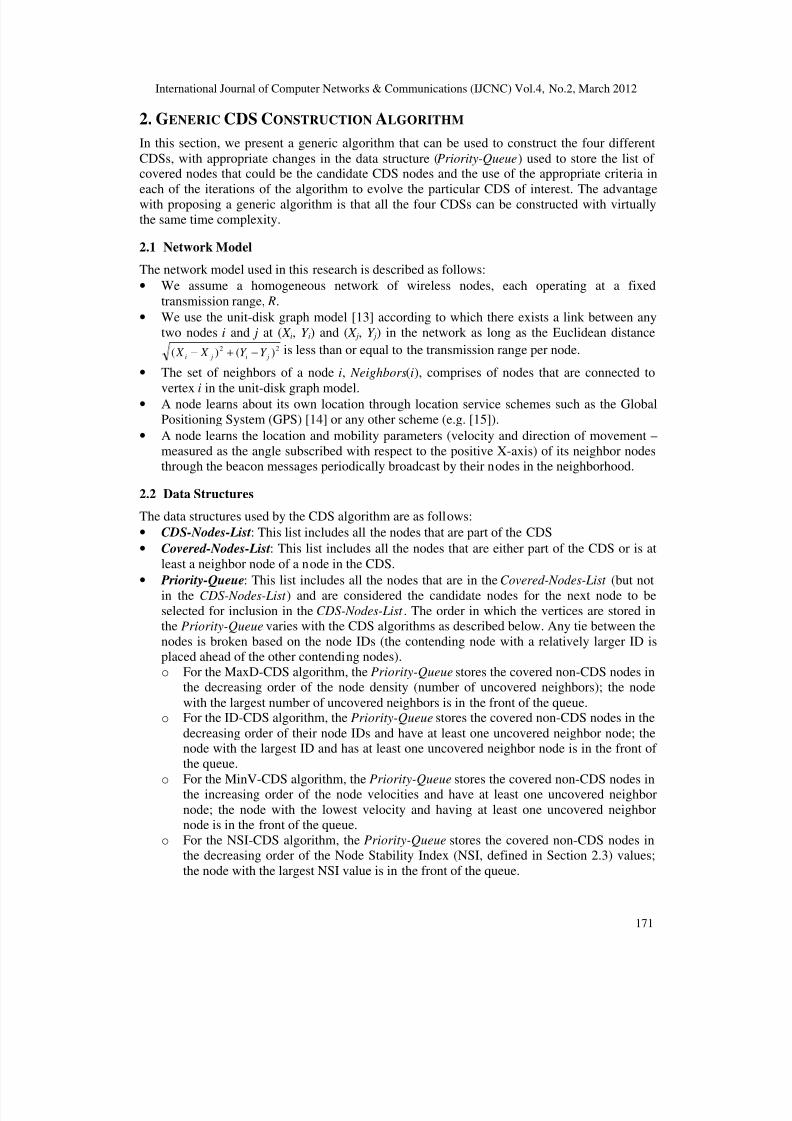
2.1 Network Model
The network model used in this research is described as follows:
• We assume a homogeneous network of wireless nodes, each operating at a fixed
transmission range, R.
• We use the unit-disk graph model [13] according to which there exists a link between any
two nodes i and j at ( X i, Y i) and ( X j, Y j) in the network as long as the Euclidean distance22
)()( ji ji Y Y X X −+− is less than or equal to the transmission range per node.
• The set of neighbors of a node i, Neighbors(i), comprises of nodes that are connected to
vertex i in the unit-disk graph model.• A node learns about its own location through location service schemes such as the Global
Positioning System (GPS) [14] or any other scheme (e.g. [15]).
• A node learns the location and mobility parameters (velocity and direction of movement –
measured as the angle subscribed with respect to the positive X-axis) of its neighbor nodesthrough the beacon messages periodically broadcast by their nodes in the neighborhood.
2.2 Data Structures
The data structures used by the CDS algorithm are as follows:
• CDS-Nodes-List: This list includes all the nodes that are part of the CDS
• Covered-Nodes-List: This list includes all the nodes that are either part of the CDS or is at
least a neighbor node of a node in the CDS.
• Priority-Queue: This list includes all the nodes that are in the Covered-Nodes-List (but not
in the CDS-Nodes-List ) and are considered the candidate nodes for the next node to be
selected for inclusion in the CDS-Nodes-List . The order in which the vertices are stored inthe Priority-Queue varies with the CDS algorithms as described below. Any tie between the
nodes is broken based on the node IDs (the contending node with a relatively larger ID isplaced ahead of the other contending nodes).
o For the MaxD-CDS algorithm, the Priority-Queue stores the covered non-CDS nodes inthe decreasing order of the node density (number of uncovered neighbors); the node
with the largest number of uncovered neighbors is in the front of the queue.o For the ID-CDS algorithm, the Priority-Queue stores the covered non-CDS nodes in the
decreasing order of their node IDs and have at least one uncovered neighbor node; thenode with the largest ID and has at least one uncovered neighbor node is in the front of the queue.
o For the MinV-CDS algorithm, the Priority-Queue stores the covered non-CDS nodes inthe increasing order of the node velocities and have at least one uncovered neighbor
node; the node with the lowest velocity and having at least one uncovered neighbornode is in the front of the queue.
o For the NSI-CDS algorithm, the Priority-Queue stores the covered non-CDS nodes inthe decreasing order of the Node Stability Index (NSI, defined in Section 2.3) values;
the node with the largest NSI value is in the front of the queue.
8/2/2019 A Simulation-Based Performance Comparison of the Minimum Node Size and Stability-Based Connected Dominating…
http://slidepdf.com/reader/full/a-simulation-based-performance-comparison-of-the-minimum-node-size-and-stability-based 4/16
International Journal of Computer Networks & Communications (IJCNC) Vol.4, No.2, March 2012
172
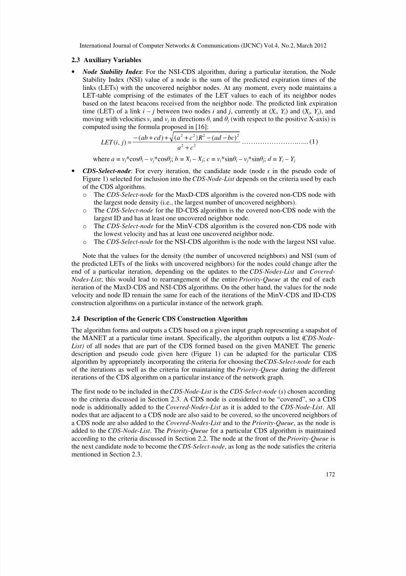
2.3 Auxiliary Variables
• Node Stability Index: For the NSI-CDS algorithm, during a particular iteration, the Node
Stability Index (NSI) value of a node is the sum of the predicted expiration times of the
links (LETs) with the uncovered neighbor nodes. At any moment, every node maintains aLET-table comprising of the estimates of the LET values to each of its neighbor nodes
based on the latest beacons received from the neighbor node. The predicted link expirationtime (LET) of a link i – j between two nodes i and j, currently at ( X i, Y i) and ( X j, Y j), andmoving with velocities vi and v j in directions θ i and θ j (with respect to the positive X-axis) is
computed using the formula proposed in [16]:
22
2222)()()(
),(ca
bcad Rcacd ab ji LET
+
−−+++−= ………………………... (1)
where a = vi*cosθ i – v j*cosθ j; b = X i – X j; c = vi*sinθ i – v j*sinθ j; d = Y i – Y j
• CDS-Select-node: For every iteration, the candidate node (node s in the pseudo code of
Figure 1) selected for inclusion into the CDS-Node-List depends on the criteria used by each
of the CDS algorithms.
o The CDS-Select-node for the MaxD-CDS algorithm is the covered non-CDS node with
the largest node density (i.e., the largest number of uncovered neighbors).o The CDS-Select-node for the ID-CDS algorithm is the covered non-CDS node with the
largest ID and has at least one uncovered neighbor node.
o The CDS-Select-node for the MinV-CDS algorithm is the covered non-CDS node withthe lowest velocity and has at least one uncovered neighbor node.
o The CDS-Select-node for the NSI-CDS algorithm is the node with the largest NSI value.
Note that the values for the density (the number of uncovered neighbors) and NSI (sum of
the predicted LETs of the links with uncovered neighbors) for the nodes could change after theend of a particular iteration, depending on the updates to the CDS-Nodes-List and Covered-
Nodes-List ; this would lead to rearrangement of the entire Priority-Queue at the end of each
iteration of the MaxD-CDS and NSI-CDS algorithms. On the other hand, the values for the nodevelocity and node ID remain the same for each of the iterations of the MinV-CDS and ID-CDS
construction algorithms on a particular instance of the network graph.
2.4 Description of the Generic CDS Construction Algorithm
The algorithm forms and outputs a CDS based on a given input graph representing a snapshot of the MANET at a particular time instant. Specifically, the algorithm outputs a list (CDS-Node-
List) of all nodes that are part of the CDS formed based on the given MANET. The genericdescription and pseudo code given here (Figure 1) can be adapted for the particular CDSalgorithm by appropriately incorporating the criteria for choosing the CDS-Select-node for each
of the iterations as well as the criteria for maintaining the Priority-Queue during the differentiterations of the CDS algorithm on a particular instance of the network graph.
The first node to be included in the CDS-Node-List is the CDS-Select-node (s) chosen accordingto the criteria discussed in Section 2.3. A CDS node is considered to be “covered”, so a CDS
node is additionally added to the Covered-Nodes-List as it is added to the CDS-Node-List . Allnodes that are adjacent to a CDS node are also said to be covered, so the uncovered neighbors of
a CDS node are also added to the Covered-Nodes-List and to the Priority-Queue, as the node isadded to the CDS-Node-List . The Priority-Queue for a particular CDS algorithm is maintained
according to the criteria discussed in Section 2.2. The node at the front of the Priority-Queue is
the next candidate node to become the CDS-Select-node, as long as the node satisfies the criteria
mentioned in Section 2.3.
8/2/2019 A Simulation-Based Performance Comparison of the Minimum Node Size and Stability-Based Connected Dominating…
http://slidepdf.com/reader/full/a-simulation-based-performance-comparison-of-the-minimum-node-size-and-stability-based 5/16
International Journal of Computer Networks & Communications (IJCNC) Vol.4, No.2, March 2012
173
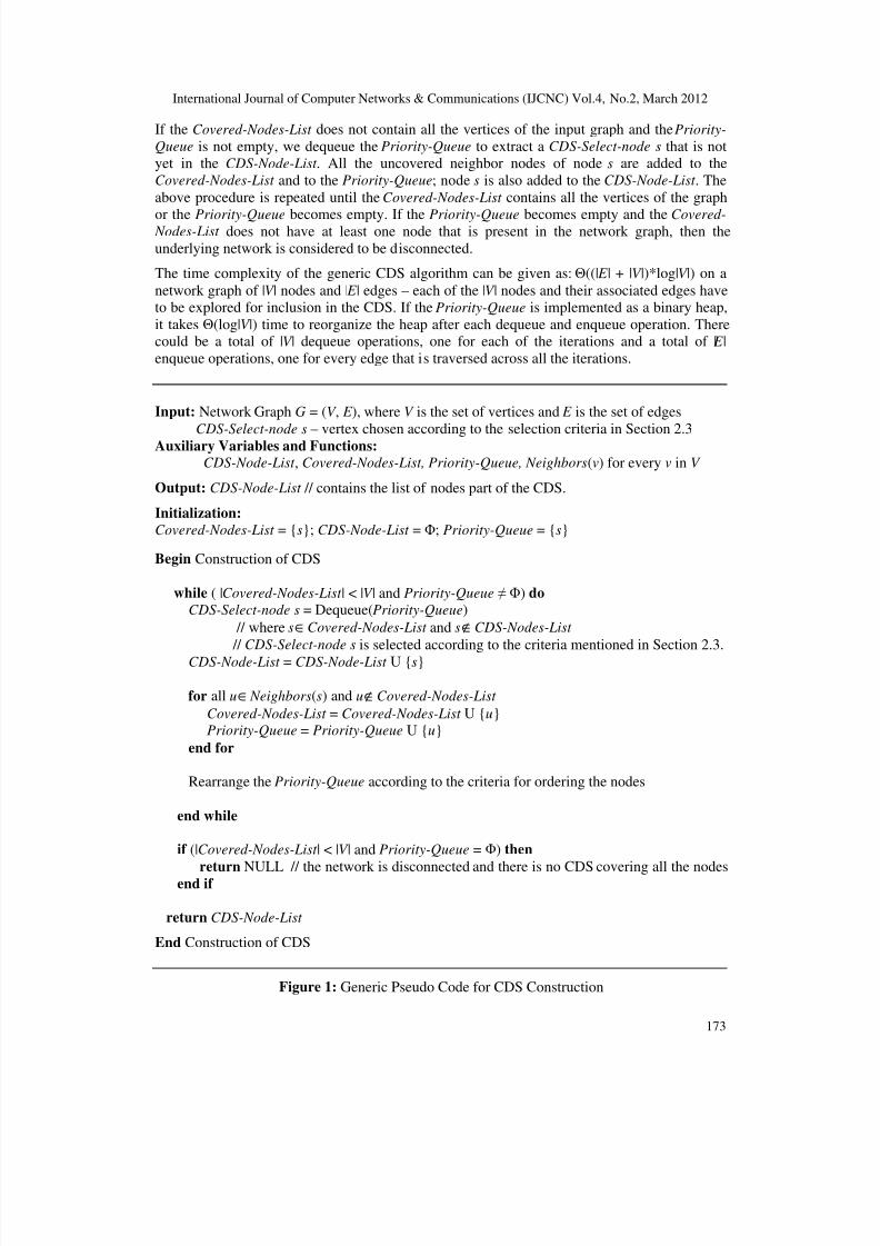
If the Covered-Nodes-List does not contain all the vertices of the input graph and the Priority-
Queue is not empty, we dequeue the Priority-Queue to extract a CDS-Select-node s that is notyet in the CDS-Node-List . All the uncovered neighbor nodes of node s are added to theCovered-Nodes-List and to the Priority-Queue; node s is also added to the CDS-Node-List . The
above procedure is repeated until the Covered-Nodes-List contains all the vertices of the graph
or the Priority-Queue becomes empty. If the Priority-Queue becomes empty and the Covered- Nodes-List does not have at least one node that is present in the network graph, then the
underlying network is considered to be disconnected.
The time complexity of the generic CDS algorithm can be given as: Θ((| E | + |V |)*log|V |) on a
network graph of |V | nodes and | E | edges – each of the |V | nodes and their associated edges haveto be explored for inclusion in the CDS. If the Priority-Queue is implemented as a binary heap,
it takes Θ(log|V |) time to reorganize the heap after each dequeue and enqueue operation. Therecould be a total of |V | dequeue operations, one for each of the iterations and a total of | E |
enqueue operations, one for every edge that is traversed across all the iterations.
Input: Network Graph G = (V , E ), where V is the set of vertices and E is the set of edges
CDS-Select-node s– vertex chosen according to the selection criteria in Section 2.3Auxiliary Variables and Functions:
CDS-Node-List , Covered-Nodes-List, Priority-Queue, Neighbors(v) for every v in V
Output: CDS-Node-List // contains the list of nodes part of the CDS.
Initialization:
Covered-Nodes-List = {s}; CDS-Node-List = Φ; Priority-Queue = {s}
Begin Construction of CDS
while ( |Covered-Nodes-List | < |V | and Priority-Queue ≠ Φ) do CDS-Select-node s = Dequeue(Priority-Queue)
// where s∈Covered-Nodes-List and s∉CDS-Nodes-List
// CDS-Select-node s is selected according to the criteria mentioned in Section 2.3.
CDS-Node-List = CDS-Node-List U {s}
for all u∈ Neighbors(s) and u∉Covered-Nodes-List
Covered-Nodes-List = Covered-Nodes-List U {u}Priority-Queue = Priority-Queue U {u}
end for
Rearrange the Priority-Queue according to the criteria for ordering the nodes
end while
if (|Covered-Nodes-List | < |V | and Priority-Queue = Φ) then
return NULL // the network is disconnected and there is no CDS covering all the nodesend if
return CDS-Node-List
End Construction of CDS
Figure 1: Generic Pseudo Code for CDS Construction
8/2/2019 A Simulation-Based Performance Comparison of the Minimum Node Size and Stability-Based Connected Dominating…
http://slidepdf.com/reader/full/a-simulation-based-performance-comparison-of-the-minimum-node-size-and-stability-based 6/16
International Journal of Computer Networks & Communications (IJCNC) Vol.4, No.2, March 2012
174
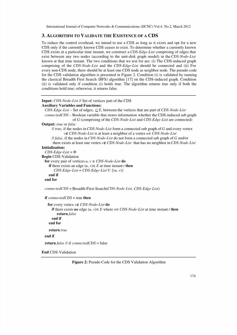
3. ALGORITHM TO VALIDATE THE EXISTENCE OF A CDS
To reduce the control overhead, we intend to use a CDS as long as it exists and opt for a new
CDS only if the currently known CDS ceases to exist. To determine whether a currently knownCDS exists at a particular time instant, we construct a CDS-Edge-List comprising of edges that
exist between any two nodes (according to the unit-disk graph model) in the CDS-Node-List
known at that time instant. The two conditions that we test for are: (i) The CDS-induced graphcomprising of the CDS-Node-List and the CDS-Edge-List should be connected and (ii) For
every non-CDS node, there should be at least one CDS node as neighbor node. The pseudo codefor the CDS validation algorithm is presented in Figure 2. Condition (i) is validated by runningthe classical Breadth First Search (BFS) algorithm [17] on the CDS-induced graph. Condition
(ii) is validated only if condition (i) holds true. The algorithm returns true only if both the
conditions hold true; otherwise, it returns false.
Input: CDS-Node-List // Set of vertices part of the CDS
Auxiliary Variables and Functions:
CDS-Edge-List – Set of edges, ⊆ E , between the vertices that are part of CDS-Node-List
connectedCDS – Boolean variable that stores information whether the CDS-induced sub graph
of G (comprising of the CDS-Node-List and CDS-Edge-List are connected)Output: true or false
// true, if the nodes in CDS-Node-List form a connected sub graph of G and every vertex
v∉CDS-Node-List is at least a neighbor of a vertex u∈CDS-Node-List
// false, if the nodes in CDS-Node-List do not form a connected sub graph of G and/or
there exists at least one vertex v∉CDS-Node-List that has no neighbor in CDS-Node-List
Initialization:CDS-Edge-List = Φ
Begin CDS-Validationfor every pair of vertices u, v ∈CDS-Node-List do
if there exists an edge (u, v)∈ E at time instant t then
CDS-Edge-List = CDS-Edge-List U {(u, v)}
end if end for
connectedCDS = Breadth-First-Search(CDS-Node-List , CDS-Edge-List )
if connectedCDS = true then
for every vertex v∉CDS-Node-List do
if there exists no edge (u, v)∈ E where u∈CDS-Node-List at time instant t then return false
end if
end for
return true
end if
return false // if connectedCDS = false
End CDS-Validation
Figure 2: Pseudo Code for the CDS Validation Algorithm
8/2/2019 A Simulation-Based Performance Comparison of the Minimum Node Size and Stability-Based Connected Dominating…
http://slidepdf.com/reader/full/a-simulation-based-performance-comparison-of-the-minimum-node-size-and-stability-based 7/16
International Journal of Computer Networks & Communications (IJCNC) Vol.4, No.2, March 2012
175
4. EXAMPLES FOR MAXD-CDS AND ID-CDS CONSTRUCTION
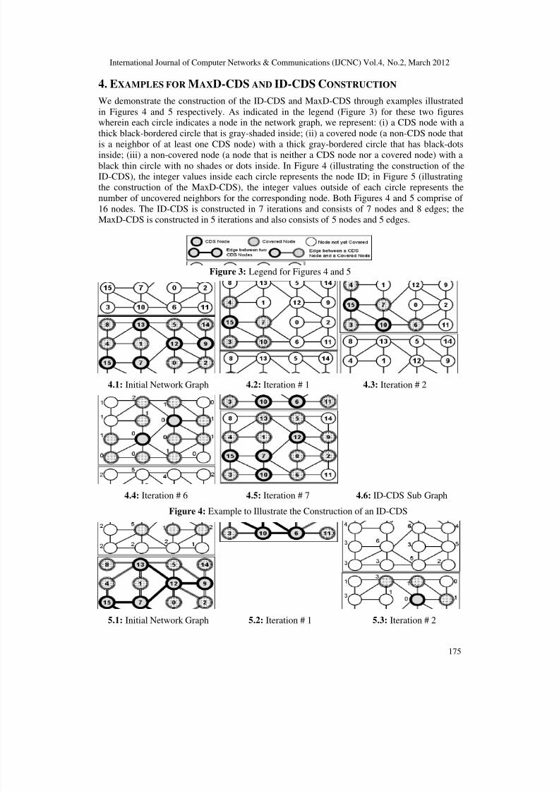
We demonstrate the construction of the ID-CDS and MaxD-CDS through examples illustrated
in Figures 4 and 5 respectively. As indicated in the legend (Figure 3) for these two figureswherein each circle indicates a node in the network graph, we represent: (i) a CDS node with a
thick black-bordered circle that is gray-shaded inside; (ii) a covered node (a non-CDS node that
is a neighbor of at least one CDS node) with a thick gray-bordered circle that has black-dotsinside; (iii) a non-covered node (a node that is neither a CDS node nor a covered node) with a
black thin circle with no shades or dots inside. In Figure 4 (illustrating the construction of theID-CDS), the integer values inside each circle represents the node ID; in Figure 5 (illustratingthe construction of the MaxD-CDS), the integer values outside of each circle represents the
number of uncovered neighbors for the corresponding node. Both Figures 4 and 5 comprise of
16 nodes. The ID-CDS is constructed in 7 iterations and consists of 7 nodes and 8 edges; theMaxD-CDS is constructed in 5 iterations and also consists of 5 nodes and 5 edges.
Figure 3: Legend for Figures 4 and 5
4.1: Initial Network Graph 4.2: Iteration # 1 4.3: Iteration # 2
4.4: Iteration # 6 4.5: Iteration # 7 4.6: ID-CDS Sub Graph
Figure 4: Example to Illustrate the Construction of an ID-CDS
5.1: Initial Network Graph 5.2: Iteration # 1 5.3: Iteration # 2
8/2/2019 A Simulation-Based Performance Comparison of the Minimum Node Size and Stability-Based Connected Dominating…
http://slidepdf.com/reader/full/a-simulation-based-performance-comparison-of-the-minimum-node-size-and-stability-based 8/16
International Journal of Computer Networks & Communications (IJCNC) Vol.4, No.2, March 2012
176
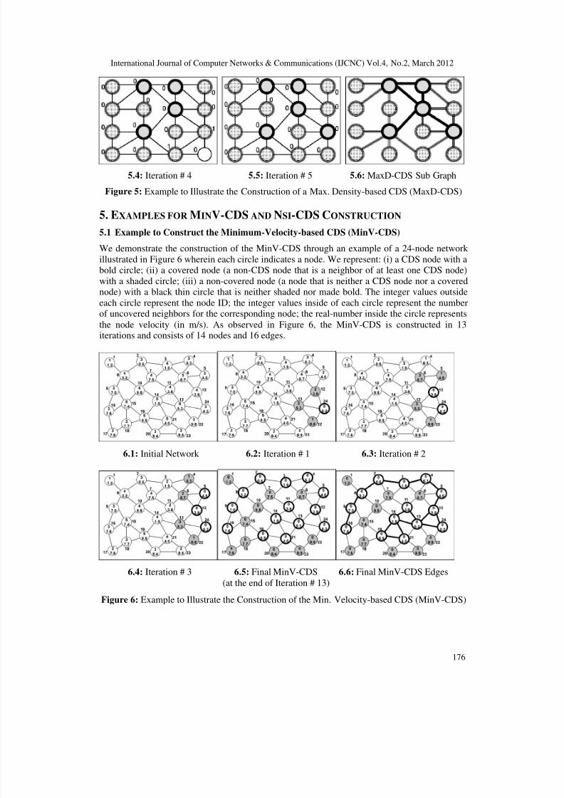
5.4: Iteration # 4 5.5: Iteration # 5 5.6: MaxD-CDS Sub Graph
Figure 5: Example to Illustrate the Construction of a Max. Density-based CDS (MaxD-CDS)
5. EXAMPLES FOR MINV-CDS AND NSI-CDS CONSTRUCTION
5.1 Example to Construct the Minimum-Velocity-based CDS (MinV-CDS)
We demonstrate the construction of the MinV-CDS through an example of a 24-node network
illustrated in Figure 6 wherein each circle indicates a node. We represent: (i) a CDS node with abold circle; (ii) a covered node (a non-CDS node that is a neighbor of at least one CDS node)
with a shaded circle; (iii) a non-covered node (a node that is neither a CDS node nor a coverednode) with a black thin circle that is neither shaded nor made bold. The integer values outside
each circle represent the node ID; the integer values inside of each circle represent the numberof uncovered neighbors for the corresponding node; the real-number inside the circle represents
the node velocity (in m/s). As observed in Figure 6, the MinV-CDS is constructed in 13iterations and consists of 14 nodes and 16 edges.
6.1: Initial Network 6.2: Iteration # 1 6.3: Iteration # 2
6.4: Iteration # 3 6.5: Final MinV-CDS 6.6: Final MinV-CDS Edges
(at the end of Iteration # 13)
Figure 6: Example to Illustrate the Construction of the Min. Velocity-based CDS (MinV-CDS)
8/2/2019 A Simulation-Based Performance Comparison of the Minimum Node Size and Stability-Based Connected Dominating…
http://slidepdf.com/reader/full/a-simulation-based-performance-comparison-of-the-minimum-node-size-and-stability-based 9/16
International Journal of Computer Networks & Communications (IJCNC) Vol.4, No.2, March 2012
177
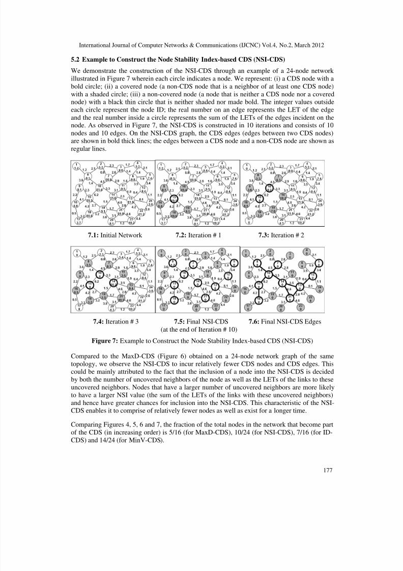
5.2 Example to Construct the Node Stability Index-based CDS (NSI-CDS)
We demonstrate the construction of the NSI-CDS through an example of a 24-node network
illustrated in Figure 7 wherein each circle indicates a node. We represent: (i) a CDS node with a
bold circle; (ii) a covered node (a non-CDS node that is a neighbor of at least one CDS node)
with a shaded circle; (iii) a non-covered node (a node that is neither a CDS node nor a covered
node) with a black thin circle that is neither shaded nor made bold. The integer values outsideeach circle represent the node ID; the real number on an edge represents the LET of the edge
and the real number inside a circle represents the sum of the LETs of the edges incident on thenode. As observed in Figure 7, the NSI-CDS is constructed in 10 iterations and consists of 10
nodes and 10 edges. On the NSI-CDS graph, the CDS edges (edges between two CDS nodes)are shown in bold thick lines; the edges between a CDS node and a non-CDS node are shown as
regular lines.
7.1: Initial Network 7.2: Iteration # 1 7.3: Iteration # 2
7.4: Iteration # 3 7.5: Final NSI-CDS 7.6: Final NSI-CDS Edges
(at the end of Iteration # 10)
Figure 7: Example to Construct the Node Stability Index-based CDS (NSI-CDS)
Compared to the MaxD-CDS (Figure 6) obtained on a 24-node network graph of the sametopology, we observe the NSI-CDS to incur relatively fewer CDS nodes and CDS edges. Thiscould be mainly attributed to the fact that the inclusion of a node into the NSI-CDS is decided
by both the number of uncovered neighbors of the node as well as the LETs of the links to these
uncovered neighbors. Nodes that have a larger number of uncovered neighbors are more likelyto have a larger NSI value (the sum of the LETs of the links with these uncovered neighbors)
and hence have greater chances for inclusion into the NSI-CDS. This characteristic of the NSI-CDS enables it to comprise of relatively fewer nodes as well as exist for a longer time.
Comparing Figures 4, 5, 6 and 7, the fraction of the total nodes in the network that become part
of the CDS (in increasing order) is 5/16 (for MaxD-CDS), 10/24 (for NSI-CDS), 7/16 (for ID-
CDS) and 14/24 (for MinV-CDS).
8/2/2019 A Simulation-Based Performance Comparison of the Minimum Node Size and Stability-Based Connected Dominating…
http://slidepdf.com/reader/full/a-simulation-based-performance-comparison-of-the-minimum-node-size-and-stability-based 10/16
International Journal of Computer Networks & Communications (IJCNC) Vol.4, No.2, March 2012
178
6. SIMULATIONS
We used our own discrete-event simulator (developed in Java) that has also been successfully
used in recent studies (e.g. [9][10][11][12]). We implemented all the four CDS algorithms(MaxD-CDS, ID-CDS, MinV-CDS and NSI-CDS) in the simulator.
6.1 Network Density
The dimensions of the network are 1000m x 1000m. Each node operates with a transmission
range of 250m. The network density is measured as the ratio N *π R2 / A, where N is the number of
nodes in the network, R is the transmission range of a node and A is the network area. We varythe network density by conducting simulations with 50 nodes (low density, corresponding to
approximately 10 neighbors per node) and 100 nodes (high density, corresponding toapproximately 20 neighbors per node).
6.2 Node Mobility Model
The well-known Random Waypoint model [18] is used as the mobility model for our
simulations. With this model, each node moves independently, from one location to another
randomly chosen location (within the network area) with a velocity uniform-randomly chosenfrom the range [0,…, vmax]. After reaching the targeted destination location, the node continuesto move to another randomly chosen location with a different randomly chosen velocity fromthe same range. We simulated three levels of node mobility by varying the vmax value – low (vmax
= 5 m/s), moderate (vmax = 25 m/s) and high (vmax = 50 m/s).
6.3 Simulation Strategy
The following simulation strategy is adopted for each of the four CDS algorithms: For every
combination of network density (50 and 100 nodes) and node mobility (vmax = 5, 25 and 50 m/s),we generate the mobility trace files for the nodes over a simulation time of 1000 seconds. Wesample (take snapshots) the network topology for every 0.25 seconds. We construct the network
graphs assuming a unit-disk graph model [13], according to which there exists a link betweenany two nodes in the network, if and only if the Euclidean distance between the two nodes is
within the transmission range of 250m. If a CDS does not exist at a particular time instant, werun the appropriate CDS algorithm and tend to use the newly determined CDS as long as itsexists (see Section 3 for the algorithm to check the existence of a CDS at any particular time
instant). We repeat the above procedure for the entire simulation time of 1000 seconds.
To measure the hop count per path, we use a list 15 source-destination (s-d ) pairs and for each s-
d pair, we run the Breadth First Search (BFS) algorithm on a CDS-induced graph (i.e., the graphcomprising of all the nodes in the network; there can be edges only between two CDS nodes and
a CDS node to a non-CDS node) generated from the network snapshot for the particular timeinstant. The source/destination roles could be assigned to any node (CDS node or non-CDS
node) in the network. A multi-hop s-d path comprises of more than one hop wherein theintermediate nodes can be only CDS nodes. Paths between two non-CDS nodes are alwaysmulti-hop in nature, even if the two non-CDS nodes are neighbors of each other. However, if
two CDS nodes or a CDS node and a non-CDS node are neighbors of each other, they cancommunicate directly.
6.4 Performance Metrics
The following performance metrics were measured in the simulations. Each metric value
represented in Figures 8 through 12 represent average of values obtained for the CDSalgorithms when simulated with 5 mobility trace files generated for every combination of
network density and node mobility.
8/2/2019 A Simulation-Based Performance Comparison of the Minimum Node Size and Stability-Based Connected Dominating…
http://slidepdf.com/reader/full/a-simulation-based-performance-comparison-of-the-minimum-node-size-and-stability-based 11/16
International Journal of Computer Networks & Communications (IJCNC) Vol.4, No.2, March 2012
179
• CDS Node Size: The time-averaged value for the number of constituent nodes of theconnected dominating sets used across the entire simulation time period. For example, if we
had used a sequence of three connected dominating sets of size 20, 18 and 25 nodes,
existing for 10, 15 and 5 seconds respectively, then the time-averaged value for the CDSNode Size is (20*10+18*15+25*5)/(10+15+5) = 19.83 and not 21 (the arithmetic average of
20, 18 and 25).• CDS Edge Size: The time-averaged value for the number of edges between the CDS nodes,
considered for each of the connected dominating sets used across the entire simulation time.
• CDS Lifetime: The average of the duration of existence of a CDS across the entire
simulation time period. The larger the CDS lifetime, the more stable it is.
• Hop Count per Path: The time-averaged value for the number of hops between source-
destination (s-d ) pairs (15 s-d pairs were considered) on paths determined on the CDS-
induced network topologies determined for every time instant across the entire simulationtime.
• CDS Node Size – Lifetime Tradeoff Ratio: A measure of the tradeoff between the two
metrics – CDS Node Size and CDS Lifetime. We desire a smaller value for the CDS NodeSize and a larger value for the CDS Lifetime. Hence, the smaller the ratio, we attribute the
CDS to have effectively balanced both these metrics, without losing out significantly on
either of them.
6.5 CDS Node Size
The MaxD-CDS and the MinV-CDS incur the lowest and largest values for the CDS Node Size.
The only objective of the MaxD-CDS algorithm is to minimize the number of nodes
constituting the CDS and it perfectly achieves this (the tradeoff being a significantly lower CDSlifetime, as discussed in Sections 6.7 and 6.8). The MinV-CDS and the ID-CDS algorithms have
no way of controlling the number of nodes becoming part of the CDS. However, the ID-CDSdoes not incur a significantly larger CDS node size and achieves about the same CDS node size
incurred by the NSI-CDS algorithm. The NSI-CDS is grouped under the category of stability-based algorithm because it is primarily designed to increase the lifetime of the CDS and it
reasonably achieves that without substantially losing out on the CDS Node Size. On the other
hand, the ID-CDS does not exist for a longer time and has to be frequently reconfigured. Sinceit does not incur significantly larger CDS node size and has a CDS Node Size – Tradeoff ratio
(see Section 6.8) close to that of the MaxD-CDS, we group the ID-CDS under minimum nodesize-based CDS algorithms. While the ID-CDS and NSI-CDS require about 40-75% more CDS
nodes (constituent nodes of the CDS) than the MaxD-CDS to cover the rest of the network nodes; the Node Size of MinV-CDS is 2.5 times or more than that of the MaxD-CDS. The
MinV-CDS algorithm primarily prefers to include the slow moving nodes to be part of the CDSand its only secondary criteria is that the CDS-Select-node has to have at least one uncovered
neighbor node. With such a design strategy, it is almost impossible to control the Node Size of aMinV-CDS. The NSI-CDS manages to have a controlled node size because the NSI of a node is
defined as the sum of the predicted LETs of the links with the neighbor nodes. Nodes with more
neighbors are more likely to have a larger NSI value and hence are likely to be included to theNSI-CDS; thus, in turn reducing the CDS Node Size.
For a given network density, the CDS Node Size incurred by the non-velocity-based algorithms
(i.e., all the three algorithms other than the MinV-CDS) is not much sensitive to the nodemobility. However, for MinV-CDS, we observe the Node Size for a MinV-CDS to increase with
increase in node mobility, especially for networks of high density (100 nodes). For a given level
of node mobility, the MaxD-CDS incurs a very minimal increase (at most 10%) in the CDSNode Size as we double the number of nodes in the network. The ID-CDS and NSI-CDS incur a
moderate increase (15-25%) in the Node Size as we double the network density. The MinV-
CDS incurs the most significant increase (20-35%) in the Node Size as we increase the number

8/2/2019 A Simulation-Based Performance Comparison of the Minimum Node Size and Stability-Based Connected Dominating…
http://slidepdf.com/reader/full/a-simulation-based-performance-comparison-of-the-minimum-node-size-and-stability-based 12/16
International Journal of Computer Networks & Communications (IJCNC) Vol.4, No.2, March 2012
180
of nodes from 50 to 100: this could be attributed to the primary focus of the MinV-CDS
algorithm being to include slow moving nodes into the CDS as long as they can cover at leastone uncovered neighbor node.
8.1: vmax = 5 m/s 8.2: vmax = 25 m/s 8.3: vmax = 50 m/s
Figure 8: Average CDS Node Size
6.6 CDS Edge Size
By virtue of incurring a lower CDS Node Size, the MaxD-CDS also incurs a lower CDS Edge
Size and the other three CDS algorithms are also ranked similar to their ranking observed for
CDS Node Size. With the distance between the MaxD-CDS nodes being close to 80% or moreof the transmission range at the time of CDS construction, the MaxD-CDS incurs relatively
fewer edges and the number of MaxD-CDS edges and MaxD-CDS nodes are close enough toeach other. In other words, the MaxD-CDS appears more like a tree; thus, the failure of evenone or a couple of edges could easily disconnect the MaxD-CDS.
9.1: vmax = 5 m/s 9.2: vmax = 25 m/s 9.3: vmax = 50 m/s
Figure 9: Average CDS Edge Size
As we include more nodes into the CDS, the number of edges between the constituent nodes of
the CDS increases almost exponentially. While the ID-CDS and NSI-CDS incur an edge size
that is within a factor of 2-4 to that of the MaxD-CDS, the MinV-CDS incurs an Edge Size thatis 15-25 times more than that incurred with the MaxD-CDS. The percentage difference in the
Edge Size for the NSI-CDS and ID-CDS for low-density networks is within 25%. The presence
of more edges between the CDS nodes has its own advantage and disadvantage: the advantageis that the CDS is more stable and does not get disconnected with a failure of one or more
edges; the disadvantage is that broadcasting through the CDS nodes and edges introducessignificant redundancy and control overhead. If one could incorporate a controlled broadcasting
by selectively using only certain CDS edges; the rest of the CDS edges could be merely used asbackup and be used for transmission and reception only when required to restore connectivity.
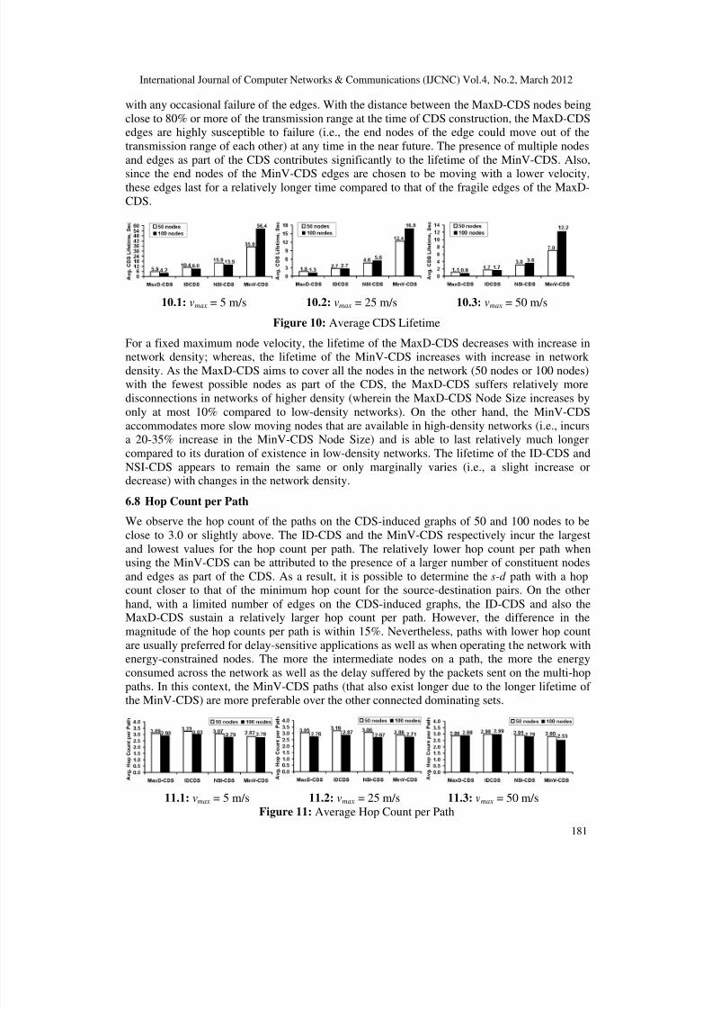
6.7 CDS Lifetime
The MaxD-CDS and MinV-CDS incur respectively the lowest and largest values for the CDS
Lifetime. We observe the ID-CDS to yield 100-200% longer lifetime than the MaxD-CDS andthe NSI-CDS has in turn been observed to last 100-200% longer than the ID-CDS; in other
words, the lifetime of the NSI-CDS is about 200-400% longer than that of the MaxD-CDS. We
observe the lifetime of the MinV-CDS to be in turn 200-400% longer than that of the NSI-CDS.Overall, with a mesh of edges, the ID-CDS and the stability-driven CDS (especially the MinV-
CDS) last significantly longer than that of the MaxD-CDS. The MaxD-CDS gets disconnected
8/2/2019 A Simulation-Based Performance Comparison of the Minimum Node Size and Stability-Based Connected Dominating…
http://slidepdf.com/reader/full/a-simulation-based-performance-comparison-of-the-minimum-node-size-and-stability-based 13/16
International Journal of Computer Networks & Communications (IJCNC) Vol.4, No.2, March 2012
181
with any occasional failure of the edges. With the distance between the MaxD-CDS nodes being
close to 80% or more of the transmission range at the time of CDS construction, the MaxD-CDSedges are highly susceptible to failure (i.e., the end nodes of the edge could move out of the
transmission range of each other) at any time in the near future. The presence of multiple nodes
and edges as part of the CDS contributes significantly to the lifetime of the MinV-CDS. Also,
since the end nodes of the MinV-CDS edges are chosen to be moving with a lower velocity,these edges last for a relatively longer time compared to that of the fragile edges of the MaxD-
CDS.
10.1: vmax = 5 m/s 10.2: vmax = 25 m/s 10.3: vmax = 50 m/s
Figure 10: Average CDS Lifetime
For a fixed maximum node velocity, the lifetime of the MaxD-CDS decreases with increase in
network density; whereas, the lifetime of the MinV-CDS increases with increase in network density. As the MaxD-CDS aims to cover all the nodes in the network (50 nodes or 100 nodes)with the fewest possible nodes as part of the CDS, the MaxD-CDS suffers relatively more
disconnections in networks of higher density (wherein the MaxD-CDS Node Size increases by
only at most 10% compared to low-density networks). On the other hand, the MinV-CDS
accommodates more slow moving nodes that are available in high-density networks (i.e., incursa 20-35% increase in the MinV-CDS Node Size) and is able to last relatively much longer
compared to its duration of existence in low-density networks. The lifetime of the ID-CDS and
NSI-CDS appears to remain the same or only marginally varies (i.e., a slight increase ordecrease) with changes in the network density.
6.8 Hop Count per Path
We observe the hop count of the paths on the CDS-induced graphs of 50 and 100 nodes to be
close to 3.0 or slightly above. The ID-CDS and the MinV-CDS respectively incur the largest
and lowest values for the hop count per path. The relatively lower hop count per path whenusing the MinV-CDS can be attributed to the presence of a larger number of constituent nodes
and edges as part of the CDS. As a result, it is possible to determine the s-d path with a hopcount closer to that of the minimum hop count for the source-destination pairs. On the other
hand, with a limited number of edges on the CDS-induced graphs, the ID-CDS and also theMaxD-CDS sustain a relatively larger hop count per path. However, the difference in the
magnitude of the hop counts per path is within 15%. Nevertheless, paths with lower hop count
are usually preferred for delay-sensitive applications as well as when operating the network withenergy-constrained nodes. The more the intermediate nodes on a path, the more the energy
consumed across the network as well as the delay suffered by the packets sent on the multi-hop
paths. In this context, the MinV-CDS paths (that also exist longer due to the longer lifetime of the MinV-CDS) are more preferable over the other connected dominating sets.
11.1: vmax = 5 m/s 11.2: vmax = 25 m/s 11.3: vmax = 50 m/sFigure 11: Average Hop Count per Path

8/2/2019 A Simulation-Based Performance Comparison of the Minimum Node Size and Stability-Based Connected Dominating…
http://slidepdf.com/reader/full/a-simulation-based-performance-comparison-of-the-minimum-node-size-and-stability-based 14/16
International Journal of Computer Networks & Communications (IJCNC) Vol.4, No.2, March 2012
182
In addition to the drawbacks of longer delay and larger network-wide energy consumption,
multi-hop paths with a larger hop count on CDS-induced graphs involving a fewer candidateintermediate nodes can be unfair to these CDS nodes. Nodes that are part of these connected
dominating sets could be relatively heavily used compared to the non-CDS nodes. This could
lead to premature failure of critical nodes, especially those located in the center of the network,
resulting in loss of network connectivity, especially in low-density networks. On the other hand,when several CDS nodes are available to serve as the intermediate nodes on multi-hop paths, we
could fairly distribute the routing load across several nodes; this could in turn enhance thefairness of node usage as well as help to incur a relatively lower end-to-end delay per data
packet due to the reduced forwarding load at these nodes.
6.9 CDS Node Size – Lifetime Tradeoff Ratio
As we observe the stability-driven connected dominating sets (MinV-CDS and NSI-CDS) to
sustain a significantly longer lifetime (compared to the MaxD-CDS and ID-CDS) at the expenseof a larger CDS Node Size, we evaluate the tradeoff between the CDS Node Size and CDS
Lifetime by calculating the ratio of these two metrics (Node Size/Lifetime) for the four
connected dominating sets. Since we prefer to have a lower CDS Node Size and a larger CDS
Lifetime, connected dominating sets that incur a lower value for the Node Size/Lifetime ratiocan be attributed to effectively balance the two metrics.
12.1: vmax = 5 m/s 12.2: vmax = 25 m/s 12.3: vmax = 50 m/s
Figure 12: CDS Node Size – Lifetime Tradeoff Ratio
Incidentally, as observed in Figure 12, the MinV-CDS is observed to have the lowest value forthis tradeoff ratio. The MinV-CDS sustains a lifetime that is 7-15 times more than the lifetimeof the MaxD-CDS, especially in high-density networks and the above said gain in the lifetime is
incurred with a Node Size that is at most 2.5 times more than that of the MaxD-CDS. However,such a large number of nodes and the resulting edges may not be preferable from the point of
view of the control overhead incurred for any broadcast communication on the CDS-inducedgraph. In this context, the NSI-CDS can be preferred for stable communication with only a verymoderately large control overhead. The NSI-CDS has a tradeoff ratio that is very much
comparable to that of the MinV-CDS. The lifetime of NSI-CDS is 2-4 times more than the
lifetime of the MaxD-CDS and the Node Size is at most 40-75% more than that of the MaxD-
CDS. The hop counts per path determined for the NSI-CDS (at most 5% larger than that of thehop counts per path using MinV-CDS) are also typically lower than that of the hop counts per
path determined using the MaxD-CDS and ID-CDS.
7. CONCLUSIONS AND FUTURE WORK We evaluated the performance of two representatives from each of the two categories of
minimum-node size driven and stability-driven connected dominating sets (CDS) for MANETs.The minimum velocity-based MinV-CDS has been observed to yield the largest lifetime, the
lowest hop count per path as well as the lowest CDS Node Size/Lifetime tradeoff ratio. The
minimum-node size based MaxD-CDS and ID-CDS are quite unstable (especially the MaxD-CDS) as well as incur a larger hop count per path. However, if the control overhead incurred in
broadcasting through a CDS with a relatively larger number of nodes and edges is a concern, the
8/2/2019 A Simulation-Based Performance Comparison of the Minimum Node Size and Stability-Based Connected Dominating…
http://slidepdf.com/reader/full/a-simulation-based-performance-comparison-of-the-minimum-node-size-and-stability-based 15/16
International Journal of Computer Networks & Communications (IJCNC) Vol.4, No.2, March 2012
183
Node Stability Index based CDS (NSI-CDS) can be considered the best choice: the NSI-CDS
sustains a significantly lower tradeoff ratio and lower hop count per path (comparable to that of the MinV-CDS) and at the same time does not incur a significantly larger Node Size. This way,
the NSI-CDS is also the most preferred candidate from the points of view of optimal energy
consumption, delay per path, bandwidth and fairness of node usage.
In addition to the detailed simulation-based evaluation of the four CDS algorithms (Maximum
density-based MaxD-CDS, Node ID-based ID-CDS, Minimum velocity-based MinV-CDS andthe Node Stability Index-based NSI-CDS), we present a generic algorithm (in the first half of
the paper) that can be used to effectively implement each of these four CDS algorithms byappropriately managing the Priority-Queue (according to the criteria used by the individual
algorithms) to store the candidate covered nodes that can be chosen for inclusion to the CDS.This way, the above four connected dominating sets can be determined with virtually the same
time complexity.
As part of future work, we will attempt to study the four CDS algorithms with respect to
mobility models other than the Random Waypoint model as well as study the applicability of the connected dominating sets for multicast communication. We will also study the energy
consumption and fairness of node usage (measured through the node lifetime) with respect to
routing (unicast and multicast) using the CDS-induced graphs vis-à-vis the unicast and multicastrouting protocols proposed for MANETs.
8. REFERENCES
[1] J. Broch, D. A. Maltz, D. B. Johnson, Y. C. Hu and J. Jetcheva, “A Performance Comparison of
Multi-hop Wireless Ad hoc Network Routing Protocols,” Proceedings of the 4th
Annual International
Conference on Mobile Computing and Networking, pp. 85-97, October 1998.
[2] P. Johansson. T. Larson, N. Hedman, B. Mielczarek and M. DegerMark, “Scenario-based
Performance Analysis of Routing Protocols for Mobile Ad hoc Networks,” Proceedings of the 5th
Annual ACM/IEEE International Conference on Mobile Computing and Networking, pp. 195-206,
August 1999.
[3] C. Siva Ram Murthy and B. S. Manoj, Ad Hoc Wireless Networks: Architectures and Protocols,Prentice Hall, 1st
Edition, June 2004.
[4] P. Sinha, R. Sivakumar and V. Bhargavan, “Enhancing Ad hoc Routing with Dynamic Virtual
Infrastructures,” Proceedings of the 20th
Annual Joint Conference of the IEEE Computer and
Communications Societies (INFOCOM), vol. 3, pp. 1763 -1772, 2001.
[5] F. Wang, M. Min, Y. Li and D. Du, “On the Construction of Stable Virtual Backbones in Mobile Ad
hoc Networks,” Proceedings of the IEEE International Performance Computing and
Communciations Conference (IPCCC), 2005.
[6] K. Sakai, M.-T. Sun and W.-S. Ku, “Maintaining CDS in Mobile Ad hoc Networks,” Wireless
Algorithms Systems and Applications, Lecture Notes in Computer Science, vol. 5258, pp. 141-153,
October 2008.
[7] P.-R. Sheu, H.-Y. Tsai, Y.-P. Lee and J. Y. Cheng, “On Calculating Stable Connected Dominating
Sets Based on Link Stability for Mobile Ad hoc Networks,” Tamkang Journal of Science and Engineering, vol. 12, no. 4, pp. 417-428, 2009.
[8] L. Bao and J. J. Garcia-Luna-Aceves, “Stable Energy-aware Topology Management in Ad hoc
Networks,” Ad hoc Networks, vol. 8, no. 3, pp. 313 – 327, May 2010.
[9] N. Meghanathan, “A Node Stability Index-based Connected Dominating Set Algorithm for MobileAd hoc Networks,” The 3
rd International Conference on Wireless & Mobile Networks, LNICST 84,
pp. 253-262, January 2012.
8/2/2019 A Simulation-Based Performance Comparison of the Minimum Node Size and Stability-Based Connected Dominating…
http://slidepdf.com/reader/full/a-simulation-based-performance-comparison-of-the-minimum-node-size-and-stability-based 16/16
International Journal of Computer Networks & Communications (IJCNC) Vol.4, No.2, March 2012
184
[10] N. Meghanathan, “An Algorithm to Determine the Sequence of Stable Connected Dominating Sets
in Mobile Ad hoc Networks,” Proceedings of the 2nd
Advanced International Conference on
Telecommunications, Guadeloupe, French Caribbean, February 2006.
[11] N. Velummylum and N. Meghanathan, “On the Utilization of ID-based Connected Dominating Sets
for Mobile Ad hoc Networks,” International Journal of Advanced Research in Computer Science ,
vol. 1, no. 3, pp. 36-43, September-October 2010.[12] N. Meghanathan, “Use of Minimum Node Velocity Based Stable Connected Dominating Sets for
Mobile Ad hoc Networks,” International Journal of Computer Applications: Special Issue on Recent
Advancements in Mobile Ad hoc Networks, vol. 2, pp. 89-96, September 2010.
[13] F. Kuhn, T. Moscibroda and R. Wattenhofer, “Unit Disk Graph Approximation,” Proceedings of the
Workshop on the Foundations of Mobile Computing ( DIALM-POMC ), pp. 17-23, October 2004.
[14] B. Hofmann-Wellenhof, H. Lichtenegger and J. Collins, Global Positioning System: Theory and
Practice, 5th
ed., Springer, September 2004.
[15] W. Keiss, H. Fuessler and J. Widmer, “Hierarchical Location Service for Mobile Ad hoc Networks,”
ACM SIGMOBILE Mobile Computing and Communications Review, vol. 8, no. 4, pp. 47-58, 2004.
[16] W. Su, S-J. Lee and M. Gerla, “Mobility Prediction and Routing in Ad hoc Wireless Networks,”
International Journal of Network Management , vol. 11, no. 1, pp. 3-30, 2001.
[17] T. H. Cormen, C. E. Leiserson, R. L. Rivest and C. Stein, Introduction to Algorithms, 3rd
Edition,
MIT Press, September 2009.
[18] C. Bettstetter, H. Hartenstein and X. Perez-Costa, “Stochastic Properties of the Random-Way Point
Mobility Model,” Wireless Networks, pp. 555-567, vol. 10, no. 5, September 2004.


