
HMM 1
A Revealing Introduction to Hidden Markov Models
Mark Stamp

HMM 2
Hidden Markov Models
What is a hidden Markov model (HMM)? A machine learning technique A discrete hill climb technique
Where are HMMs used? Speech recognition Malware detection, IDS, etc., etc.
Why is it useful? Efficient algorithms

HMM 3
Markov Chain
Markov chain is a “memoryless random process”
Transitions depend only on current state and transition probabilities matrix
Example on next slide…

HMM 4
Markov Chain
We are interested in average annual temperature Only consider Hot and Cold
From recorded history, we obtain probabilities See diagram to the right
H
C
0.7
0.6
0.3 0.4

HMM 5
Markov Chain
Transition probability matrix
Matrix is denoted as A
Note, A is “row stochastic”
H
C
0.7
0.6
0.3 0.4

HMM 6
Markov Chain
Can also include begin, end states
Begin state matrix is π In this example,
Note that π is row stochastic
H
C
0.7
0.6
0.3 0.4begin end
0.6
0.4

HMM 7
Hidden Markov Model
HMM includes a Markov chain But this Markov process is “hidden”
Cannot observe the Markov process Instead, we observe something related
to hidden states It’s as if there is a “curtain” between
Markov chain and observations Example on next slide

HMM 8
HMM Example
Consider H/C temperature example Suppose we want to know H or C
temperature in distant past Before humans (or thermometers)
invented OK if we can just decide Hot versus Cold
We assume transition between Hot and Cold years is same as today That is, the A matrix is same as today

HMM 9
HMM Example
Temp in past determined by Markov process But, we cannot observe temperature in past Instead, we note that tree ring size is
related to temperature Look at historical data to see the connection
We consider 3 tree ring sizes Small, Medium, Large (S, M, L, respectively)
Measure tree ring sizes and recorded temperatures to determine relationship

HMM 10
HMM Example
We find that tree ring sizes and temperature related by
This is known as the B matrix:
Note that B also row stochastic
HMM 11
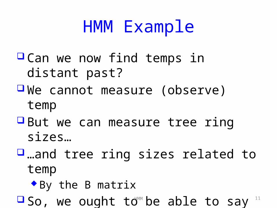
HMM Example
Can we now find temps in distant past?
We cannot measure (observe) temp But we can measure tree ring sizes… …and tree ring sizes related to temp
By the B matrix So, we ought to be able to say
something about temperature

HMM 12
HMM Notation
A lot of notation is required Notation may be the most difficult part

HMM 13
HMM Notation
To simplify notation, observations are taken from the set {0,1,…,M-1}
That is, The matrix A = {aij} is N x N, where
The matrix B = {bj(k)} is N x M,
where

HMM 14
HMM Example
Consider our temperature example… What are the observations?
V = {0,1,2}, which corresponds to S,M,L What are states of Markov process?
Q = {H,C} What are A,B, π, and T?
A,B, π on previous slides T is number of tree rings measured
What are N and M? N = 2 and M = 3
HMM 15
Generic HMM
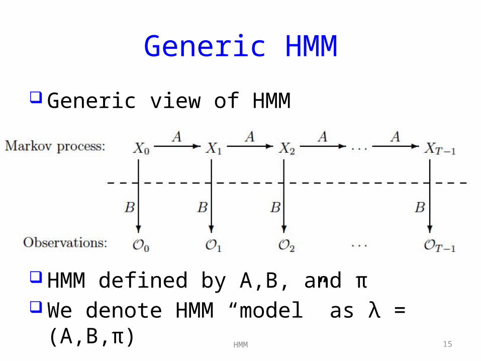
Generic view of HMM
HMM defined by A,B, and π We denote HMM “model” as λ =
(A,B,π)

HMM 16
HMM Example
Suppose that we observe tree ring sizes For 4 year period of interest: S,M,S,L Then = (0, 1, 0, 2)
Most likely (hidden) state sequence? We want most likely X = (x0, x1, x2, x3)
Let πx0 be prob. of starting in state x0
Note prob. of initial observation And ax0,x1 is prob. of transition x0 to x1
And so on…

HMM 17
HMM Example
Bottom line? We can compute P(X) for any X For X = (x0, x1, x2, x3) we have
Suppose we observe (0,1,0,2), then what is probability of, say, HHCC?
Plug into formula above to find

HMM 18
HMM Example
Do same for all 4-state sequences
We find… The winner is?
CCCH Not so fast my
friend…

HMM 19
HMM Example
The path CCCH scores the highest In dynamic programming (DP), we
find highest scoring path But, HMM maximizes expected
number of correct states Sometimes called “EM algorithm” For “Expectation Maximization”
How does HMM work in this example?

HMM 20
HMM Example
For first position… Sum probabilities for all paths that have
H in 1st position, compare to sum of probs for paths with C in 1st position --- biggest wins
Repeat for each position and we find:

HMM 21
HMM Example
So, HMM solution gives us CHCH While dynamic program solution is CCCH Which solution is better? Neither!!! Why is that?
Different definitions of “best”

HMM 22
HMM Paradox?
HMM maximizes expected number of correct states Whereas DP chooses “best” overall path
Possible for HMM to choose “path” that is impossible Could be a transition probability of 0
Cannot get impossible path with DP Is this a flaw with HMM?
No, it’s a feature…

HMM 23
The Three Problems
HMMs used to solve 3 problems Problem 1: Given a model λ = (A,B,π) and
observation sequence O, find P(O|λ) That is, we score an observation sequence to see
how well it fits the given model Problem 2: Given λ = (A,B,π) and O, find an
optimal state sequence Uncover hidden part (as in previous example)
Problem 3: Given O, N, and M, find the model λ that maximizes probability of O That is, train a model to fit the observations

HMM 24
HMMs in Practice
Typically, HMMs used as follows Given an observation sequence Assume a hidden Markov process exists Train a model based on observations
Problem 3 (determine N by trial and error) Then given a sequence of observations,
score it vs model from previous step Problem 1 (high score implies it’s similar to
training data)

HMM 25
HMMs in Practice
Previous slide gives sense in which HMM is a “machine learning” technique We do not need to specify anything except
the parameter N And “best” N found by trial and error
That is, we don’t have to think too much Just train HMM and then use it Best of all, efficient algorithms for HMMs
HMM 26
The Three Solutions
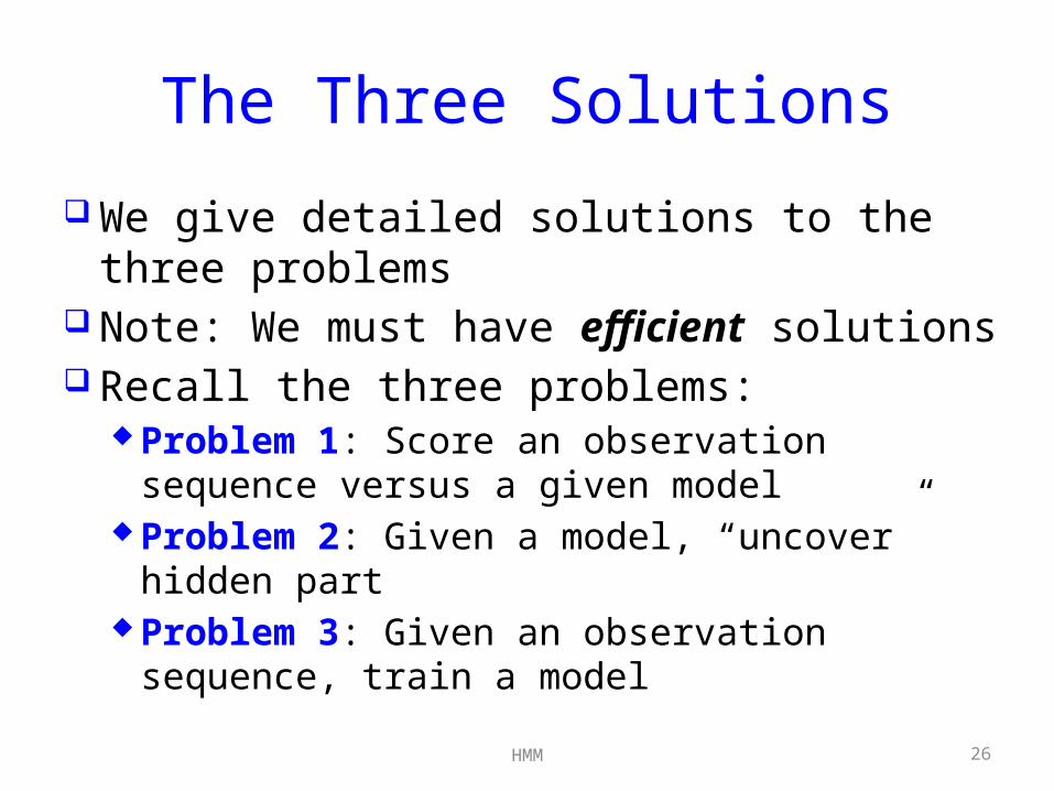
We give detailed solutions to the three problems
Note: We must have efficient solutions Recall the three problems:
Problem 1: Score an observation sequence versus a given model
Problem 2: Given a model, “uncover” hidden part
Problem 3: Given an observation sequence, train a model

HMM 27
Solution 1
Score observations versus a given model Given model λ = (A,B,π) and observation
sequence O=(O0,O1,…,OT-1), find P(O|λ)
Denote hidden states as X = (x0, x1, . . . , xT-1)
Then from definition of B,P(O|X,λ)=bx0(O0) bx1(O1) … bxT-1(OT-1)
And from definition of A and π,P(X|λ)=πx0 ax0,x1 ax1,x2 … axT-2,xT-1

HMM 28
Solution 1
Elementary conditional probability fact:P(O,X|λ) = P(O|X,λ) P(X|λ)
Sum over all possible state sequences X,P(O|λ) = Σ P(O,X|λ) = Σ P(O|X,λ) P(X|λ)= Σπx0bx0(O0)ax0,x1bx1(O1)…axT-2,xT-1bxT-1(OT-1)
This “works” but way too costly Requires about 2TNT multiplications
Why? There better be a better way…

HMM 29
Forward Algorithm
Instead of brute force: forward algorithm Or “alpha pass”
For t = 0,1,…,T-1 and i=0,1,…,N-1, letαt(i) = P(O0,O1,…,Ot,xt=qi|λ)
Probability of “partial sum” to t, and Markov process is in state qi at step t What the?
Can be computed recursively, efficiently
HMM 30
Forward Algorithm
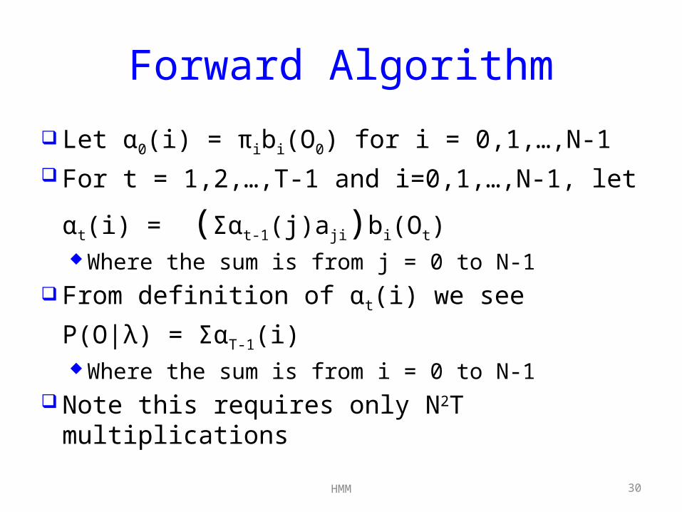
Let α0(i) = πibi(O0) for i = 0,1,…,N-1 For t = 1,2,…,T-1 and i=0,1,…,N-1, let
αt(i) = (Σαt-1(j)aji)bi(Ot) Where the sum is from j = 0 to N-1
From definition of αt(i) we see
P(O|λ) = ΣαT-1(i) Where the sum is from i = 0 to N-1
Note this requires only N2T multiplications
HMM 31
Solution 2
Given a model, find “most likely” hidden states: Given λ = (A,B,π) and O, find an optimal state sequence Recall that optimal means “maximize
expected number of correct states” In contrast, DP finds best scoring path
For temp/tree ring example, solved this But hopelessly inefficient approach
A better way: backward algorithm Or “beta pass”

HMM 32
Backward Algorithm
For t = 0,1,…,T-1 and i=0,1,…,N-1, letβt(i) = P(Ot+1,Ot+2,…,OT-1|xt=qi,λ)
Probability of partial sum from t to end and Markov process in state qi at step t
Analogous to the forward algorithm As with forward algorithm, this can be
computed recursively and efficiently

HMM 33
Backward Algorithm
Let βT-1(i) = 1 for i = 0,1,…,N-1 For t = T-2,T-3, …,1 and i=0,1,…,N-1,
letβt(i) = Σai,jbj(Ot+1)βt+1(j) Where the sum is from j = 0 to N-1

HMM 34
Solution 2
For t = 1,2,…,T-1 and i=0,1,…,N-1 defineγt(i) = P(xt=qi|O,λ) Most likely state at t is qi that maximizes γt(i)
Note that γt(i) = αt(i)βt(i)/P(O|λ) And recall P(O|λ) = ΣαT-1(i)
The bottom line? Forward algorithm solves Problem 1 Forward/backward algorithms solve Problem 2

HMM 35
Solution 3
Train a model: Given O, N, and M, find λ that maximizes probability of O
Here, we iteratively adjust λ = (A,B,π) to better fit the given observations O The size of matrices are fixed (N and M) But elements of matrices can change
It is amazing that this works! And even more amazing that it’s
efficient

HMM 36
Solution 3
For t=0,1,…,T-2 and i,j in {0,1,…,N-1}, define “di-gammas” asγt(i,j) = P(xt=qi, xt+1=qj|O,λ)
Note γt(i,j) is prob of being in state qi at time t and transiting to state qj at t+1
Then γt(i,j) = αt(i)aijbj(Ot+1)βt+1(j)/P(O|λ) And γt(i) = Σγt(i,j)
Where sum is from j = 0 to N – 1
HMM 37
Model Re-estimation
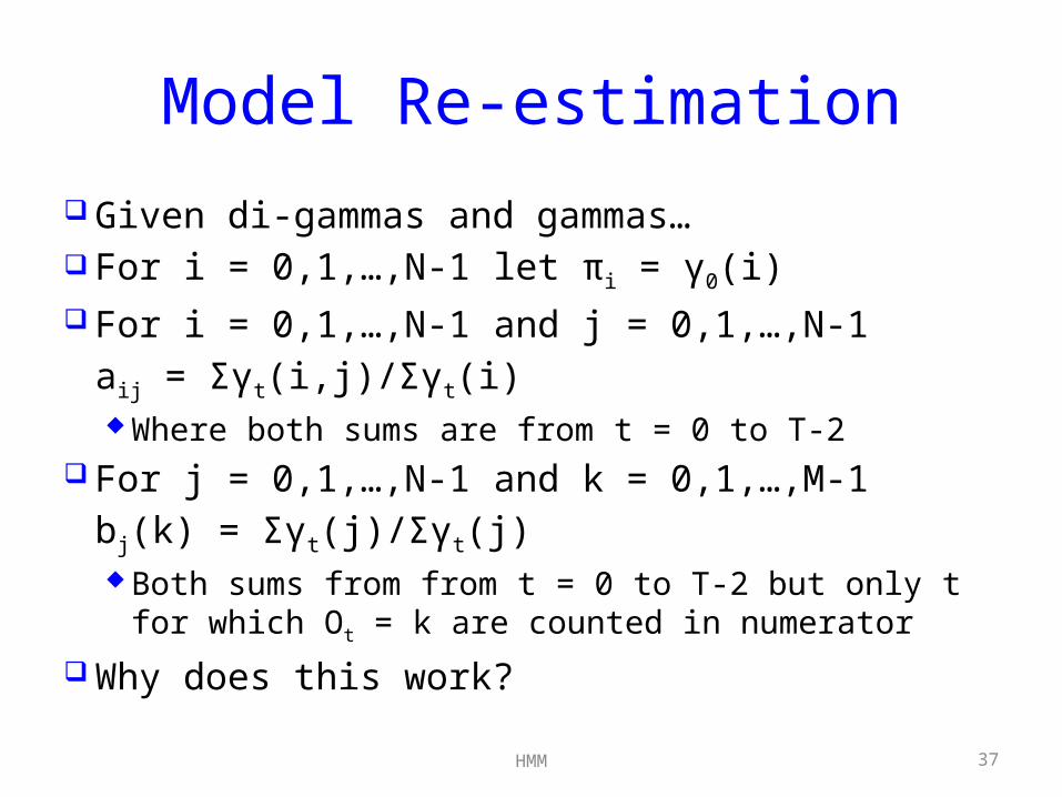
Given di-gammas and gammas… For i = 0,1,…,N-1 let πi = γ0(i) For i = 0,1,…,N-1 and j = 0,1,…,N-1
aij = Σγt(i,j)/Σγt(i) Where both sums are from t = 0 to T-2
For j = 0,1,…,N-1 and k = 0,1,…,M-1 bj(k) = Σγt(j)/Σγt(j) Both sums from from t = 0 to T-2 but only t for
which Ot = k are counted in numerator
Why does this work?
HMM 38
Solution 3
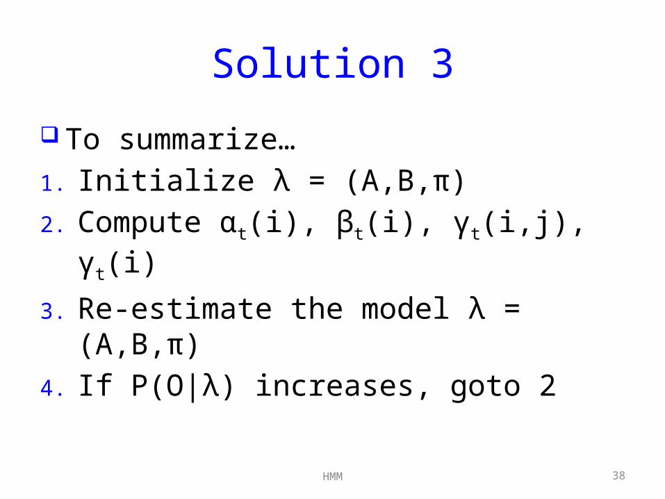
To summarize…1. Initialize λ = (A,B,π) 2. Compute αt(i), βt(i), γt(i,j), γt(i)
3. Re-estimate the model λ = (A,B,π) 4. If P(O|λ) increases, goto 2

HMM 39
Solution 3
Some fine points… Model initialization
If we have a good guess for λ = (A,B,π) then we can use it for initialization
If not, let πi ≈ 1/N, ai,j ≈ 1/N, bj(k) ≈ 1/M Subject to row stochastic conditions Note: Do not initialize to uniform values
Stopping conditions Stop after some number of iterations Stop if increase in P(O|λ) is “small”
HMM 40
HMM as Discrete Hill Climb
Algorithm on previous slides shows that HMM is a “discrete hill climb”
HMM consists of discrete parameters Specifically, the elements of the matrices
And re-estimation process improves model by modifying parameters So, process “climbs” toward improved model This happens in a high-dimensional space

HMM 41
Dynamic Programming
Brief detour… For λ = (A,B,π) as above, it’s easy to
define a dynamic program (DP) Executive summary:
DP is forward algorithm, with “sum” replaced by “max”
Precise details on next slides

HMM 42
Dynamic Programming
Let δ0(i) = πi bi(O0) for i=0,1,…,N-1 For t=1,2,…,T-1 and i=0,1,…,N-1 compute
δt(i) = max (δt-1(j)aji)bi(Ot) Where the max is over j in {0,1,…,N-1}
Note that at each t, the DP computes best path for each state, up to that point
So, probability of best path is max δT-1(j) This max only gives best probability
Not the best path, for that, see next slide

HMM 43
Dynamic Programming
To determine optimal path While computing optimal path, keep track
of pointers to previous state When finished, construct optimal path by
tracing back points For example, consider temp example Probabilities for path of length 1:
These are the only “paths” of length 1

HMM 44
Dynamic Programming
Probabilities for each path of length 2
Best path of length 2 ending with H is CH
Best path of length 2 ending with C is CC

HMM 45
Dynamic Program
Continuing, we compute best path ending at H and C at each step
And save pointers --- why?

HMM 46
Dynamic Program
Best final score is .002822 And, thanks to pointers, best path is CCCH
But what about underflow? A serious problem in bigger cases

HMM 47
Underflow Resistant DP
Common trick to prevent underflow Instead of multiplying probabilities… …we add logarithms of probabilities
Why does this work? Because log(xy) = log x + log y And adding logs does not tend to 0
Note that we must avoid 0 probabilities

HMM 48
Underflow Resistant DP
Underflow resistant DP algorithm: Let δ0(i) = log(πi bi(O0)) for i=0,1,…,N-1 For t=1,2,…,T-1 and i=0,1,…,N-1 compute
δt(i) = max (δt-1(j) + log(aji) + log(bi(Ot))) Where the max is over j in {0,1,…,N-1}
And score of best path is max δT-1(j) As before, must also keep track of paths

HMM 49
HMM Scaling
Trickier to prevent underflow in HMM We consider solution 3
Since it includes solutions 1 and 2 Recall for t = 1,2,…,T-1, i=0,1,…,N-1,
αt(i) = (Σαt-1(j)aj,i)bi(Ot) The idea is to normalize alphas so
that they sum to one Algorithm on next slide

HMM 50
HMM Scaling
Given αt(i) = (Σαt-1(j)aj,i)bi(Ot) Let a0(i) = α0(i) for i=0,1,…,N-1 Let c0 = 1/Σa0(j) For i = 0,1,…,N-1, let a0(i) = c0a0(i) This takes care of t = 0 case Algorithm continued on next slide…

HMM 51
HMM Scaling
For t = 1,2,…,T-1 do the following: For i = 0,1,…,N-1,
at(i) = (Σat-1(j)aj,i)bi(Ot) Let ct = 1/Σat(j) For i = 0,1,…,N-1 let at(i) = ctat(i)

HMM 52
HMM Scaling
Easy to show at(i) = c0c1…ct αt(i) (♯) Simple proof by induction
So, c0c1…ct is scaling factor at step t Also, easy to show that
at(i) = αt(i)/Σαt(j) Which implies ΣaT-1(i) = 1
(♯♯)

HMM 53
HMM Scaling
By combining (♯) and (♯♯), we have1 = ΣaT-1(i) = c0c1…cT-1 ΣαT-1(i)
= c0c1…cT-1
P(O|λ) Therefore, P(O|λ) = 1 / c0c1…cT-1
To avoid underflow, we computelog P(O|λ) = -Σ log(cj) Where sum is from j = 0 to T-1

HMM 54
HMM Scaling
Similarly, scale betas as ctβt(i) For re-estimation,
Compute γt(i,j) and γt(i) using original formulas, but with scaled alphas and betas
This gives us new values for λ = (A,B,π) “Easy exercise” to show re-estimate is exact
when scaled alphas and betas used Also, P(O|λ) cancels from formula
Use log P(O|λ) = -Σ log(cj) to decide if iterate improves

HMM 55
All Together Now
Complete pseudo code for Solution 3 Given: (O0,O1,…,OT-1) and N and M Initialize: λ = (A,B,π)
A is NxN, B is NxM and π is 1xN πi ≈ 1/N, aij ≈ 1/N, bj(k) ≈ 1/M, each matrix row
stochastic, but not uniform Initialize:
maxIters = max number of re-estimation steps iters = 0 oldLogProb = -∞

HMM 56
Forward Algorithm
Forward algorithm With scaling
HMM 57
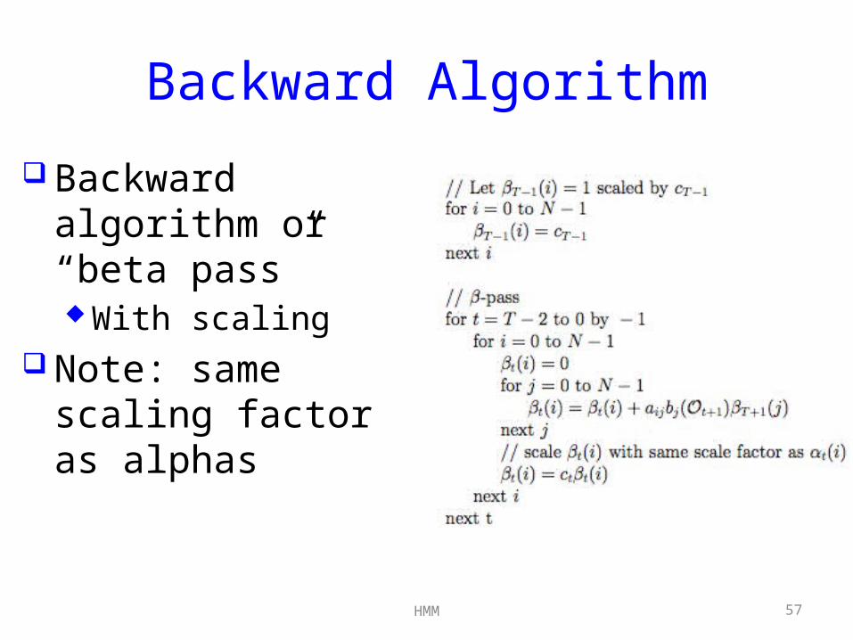
Backward Algorithm
Backward algorithm or “beta pass” With scaling
Note: same scaling factor as alphas
HMM 58
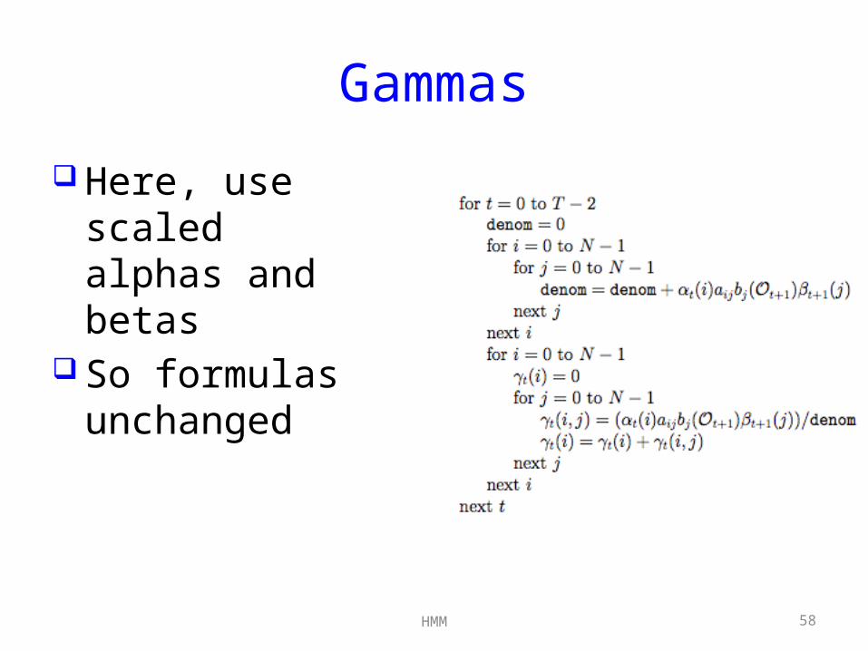
Gammas
Here, use scaled alphas and betas
So formulas unchanged
HMM 59
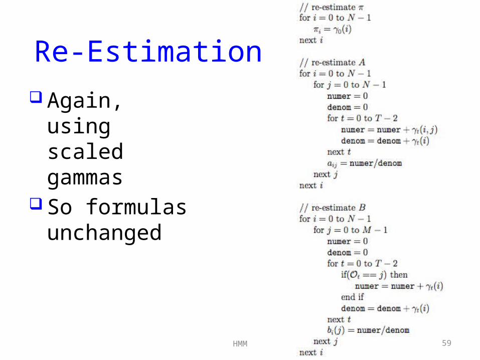
Re-Estimation Again, using
scaled gammas
So formulas unchanged

HMM 60
Stopping Criteria
Check that probability increases In practice, wantlogProb >
oldLogProb + ε And don’t
exceed max iterations

HMM 61
English Text Example
Suppose Martian arrives on earth Sees written English text Wants to learn something about it Martians know about HMMs
So, strip our all non-letters, make all letters lower-case 27 symbols (letters, plus word-space) Train HMM on long sequence of symbols

HMM 62
English Text
For first training case, initialize: N = 2 and M = 27 Elements of A and π are about ½ each Elements of B are each about 1/27
We use 50,000 symbols for training After 1st iter: log P(O|λ) ≈ -165097 After 100th iter: log P(O|λ) ≈ -137305

HMM 63
English Text
Matrices A and π converge:
What does this tells us? Started in hidden state 1 (not state 0) And we know transition probabilities
between hidden states Nothing too interesting here
We don’t care about hidden states

HMM 64
English Text
What about B matrix?
This much more interesting… Why???
HMM 65
A Security Application
Suppose we want to detect metamorphic computer viruses Such viruses vary their internal structure But function of malware stays same If sufficiently variable, standard signature
detection will fail Can we use HMM for detection?
What to use as observation sequence? Is there really a “hidden” Markov process? What about N, M, and T? How many Os needed for training, scoring?

HMM 66
HMM for Metamorphic Detection
Set of “family” viruses into 2 subsets Extract opcodes from each virus Append opcodes from subset 1 to make one
long sequence Train HMM on opcode sequence (problem 3) Obtain a model λ = (A,B,π)
Set threshold: score opcodes from files in subset 2 and “normal” files (problem 1) Can you sets a threshold that separates sets? If so, may have a viable detection method

HMM 67
HMM for Metamorphic Detection
Virus detection results from recent paper Note the
separation This is
good!

HMM 68
HMM Generalizations
Here, assumed Markov process of order 1 Current state depends only on previous state
and transition matrix Can use higher order Markov process
Current state depends on n previous states Higher order vs increased N ?
Can have A and B matrices depend on t HMM often combined with other
techniques (e.g., neural nets)

HMM 69
Generalizations
In some cases, big limitation of HMM is that position information is not used In many applications this is OK/desirable In some apps, this is a serious limitation
Bioinformatics applications DNA sequencing, protein alignment, etc. Sequence alignment is crucial They use “profile HMMs” instead of HMMs PHMM is next topic…

HMM 70
References
A revealing introduction to hidden Markov models, by M. Stamp http://www.cs.sjsu.edu/faculty/stamp/RU
A/HMM.pdf A tutorial on hidden Markov models
and selected applications in speech recognition, by L.R. Rabiner http://www.cs.ubc.ca/~murphyk/Bayes/r
abiner.pdf

HMM 71
References
Hunting for metamorphic engines, W. Wong and M. Stamp Journal in Computer Virology, Vol. 2, No.
3, December 2006, pp. 211-229 Hunting for undetectable
metamorphic viruses, D. Lin and M. Stamp Journal in Computer Virology, Vol. 7, No.
3, August 2011, pp. 201-214


