Download - A preliminary investigation on an ELLAM scheme for linear transport equations

A Preliminary Investigation on an ELLAM Schemefor Linear Transport EquationsMohamed Al-Lawatia,1 Hong Wang2

1Department of Mathematics and Statistics, Sultan Qaboos University, P.O. Box 36,Al-Khod Postal Code 123, Muscat, Sultanate of Oman

2Department of Mathematics, University of South Carolina, Columbia,South Carolina 29208

Received 7 August 2001; accepted 15 June 2002

DOI 10.1002/num.10042

We present an Eulerian-Lagrangian localized adjoint method (ELLAM) for linear advection-reaction partialdifferential equations in multiple space dimensions. We carry out numerical experiments to investigate theperformance of the ELLAM scheme with a range of well-perceived and widely used methods in fluid dynamicsincluding the monotonic upstream-centered scheme for conservation laws (MUSCL), the minmod method, theflux-corrected transport method (FCT), and the essentially non-oscillatory (ENO) schemes and weightedessentially non-oscillatory (WENO) schemes. These experiments show that the ELLAM scheme is verycompetitive with these methods in the context of linear transport PDEs, and suggest/justify the development ofELLAM-based simulators for subsurface porous medium flows and other applications. © 2002 Wiley Periodicals,Inc. Numer Methods Partial Differential Eq 19: 22–43, 2003

Keywords: advection-reaction equations; characteristic methods; comparison of numerical methods;essentially nonoscillatory schemes; Eulerian-Lagrangian methods; transport equations

I. INTRODUCTION

Advection-dominated transport partial differential equations (PDEs) describe the displacementof oil by an injected fluid in petroleum recovery, subsurface contaminant transport andremediation, and many other applications. The mathematical models used to describe thesecomplex flow processes are coupled systems of time-dependent nonlinear PDEs and constrain-ing equations. The numerical simulation of these systems presents severe numerical difficulties[1–3]. One of the major difficulties in the numerical simulation to these coupled systems is an

Correspondence to: Hong Wang, University of South Carolina, Department of Mathematics, Columbia, SC 29208(e-mail: [email protected])Contract grant sponsors: Mobil Technology Company and ExxonMobil Upstream Research CompanyContract grant sponsor: South Carolina State Commission of Higher Education, South Carolina Research InitiativeGrant.Contract grant sponsor: National Science Foundation; contract grant number: DMS-0079549

© 2002 Wiley Periodicals, Inc.

accurate and efficient solution of the advection-dominated transport PDE for the concentration,which is virtually linear in terms of its primary unknown when the fluids are fully miscible.Standard finite difference or finite element methods (FDMs, FEMs) tend to generate solutionswith severe nonphysical oscillations. Although classical upwind FDM could eliminate theseoscillations, it yields solutions with excessive smearing and potentially spurious effects relatedto the orientation of the grid. A huge variety of improved methods have been developed to solveadvection-dominated PDEs.

Most of these methods use fixed spatial grids with some form of upstream weighting and thestandard temporal discretization. The optimal test function methods [4–6] attempt to minimizespatial errors and yield an upstream bias in the resulting numerical schemes. Hence, they aresusceptible to time truncation errors that introduce numerical dispersion and the restrictions onthe size of time steps. They tend to be ineffective for transient advection-dominated problems.Some other methods [7–9] attempt to reduce the local truncation errors by using nonzero spatialerrors to cancel temporal errors. The streamline diffusion finite element methods (SDFEMs) [10,11] add a numerical diffusion only in the direction of streamlines with no crosswind diffusionintroduced. Many high-resolution methods, such as the total variation diminishing methods(TVD) and the essentially nonoscillatory (ENO) methods [12–16] are based on Godunovmethods [17] and are well suited for the solution of nonlinear hyperbolic conservation laws.They resolve shock discontinuities in the solutions of hyperbolic conservation laws withoutexcessive smearing or spurious oscillations. Moreover, they conserve mass; this property is ofessential importance in applications.

Because of the hyperbolic nature of advective transport, characteristic methods have beensuccessfully applied to solve linear transport PDEs [18–22]. Characteristic methods carry outthe temporal discretization by following the movement of particles along the streamlines.Because the solutions of transport PDEs are much smoother along the characteristics than theyare in the time direction, characteristic methods generate accurate solutions even if very largetime steps are used. However, characteristic methods raise many implementational and analyt-ical issues that need to be addressed. Traditional particle tracking methods advance the gridsfollowing the characteristics. They greatly reduce temporal errors and, thus, generate fairlyaccurate solutions. However, they often severely distort the evolving grids and greatly compli-cate the solution procedures. The modified method of characteristics (MMOC) [19] follows theflow direction by tracking the characteristics backward from a fixed grid at the current time stepand hence, avoids the grid distortion problems present in forward tracking methods. The MMOCsymmetrizes and stabilizes the governing PDEs, and greatly reduces temporal errors. It allowsfor large time steps in a simulation without loss of accuracy and eliminates the excessivenumerical dispersion and grid orientation effects. The major drawbacks of many previouscharacteristic methods are that they fail to conserve mass and have difficulties in treating generalboundary conditions.

The Eulerian-Lagrangian localized adjoint method (ELLAM) was introduced by Celia et al.in solving (one-dimensional constant-coefficient) advection-diffusion PDEs [23] and was thengeneralized to solve linear advection-reaction transport PDEs [24, 25]. The ELLAM method-ology provides a general characteristic solution procedure and a consistent framework fortreating general boundary conditions and conserving mass. Thus, it overcomes the two principalshortcomings of the previous characteristic methods while maintaining their numerical advan-tages. In this article we present an ELLAM for multidimensional linear advection-reactiontransport PDEs. We then carry out numerical experiments to compare the performance of theELLAM scheme with high-resolution methods in the context of linear advection-reactiontransport PDEs, including the monotonic upstream-centered scheme for conservation laws

AN INVESTIGATION OF AN ELLAM SCHEME 23

(MUSCL), the minmod scheme, the flux-corrected transport method (FCT), and the essentiallynonoscillatory (ENO) and the weighted ENO (WENO) schemes [12–14, 16, 26–29].

The rest of the article is organized as follows: In Section 2 we present an ELLAM scheme.In Section 3 we briefly recall the MUSCL, minmod, FCT, ENO, and WENO schemes. InSection 4 we conduct numerical experiments to investigate the performance of the ELLAM andthese methods. Section 5 contains summary and discussions.

II. AN ELLAM SCHEMEA. Definition of Test Functions

We consider a multidimensional linear advection-reaction PDE

ct � � � �vc�x, t�� K�x, t�c � F�x, t�, x � �, t � �0, T�,

c�x, t� � g�x, t�, �x, t� � ��I� � �0, T� (2.1)

where � � �d is a bounded domain with a Lipschitz continuous boundary � � ��. A boundarycondition is specified at the inflow boundary �(I) identified by �(I) � {x�x � �, v � n 0}. Inaddition, an initial condition c(x, 0) � c0(x) is specified to close the problem (2.1).

We define a quasi-uniform temporal partition on [0, T] by 0 � t0 t1 t2 . . . tN1

tN � T. Multiplying Eq. (2.1) by space-time test functions w(x, t) that are continuous andpiecewise smooth, vanish outside the space-time strip � � [tn1, tn], and are discontinuous intime at time tn1, we obtain a space-time weak formulation

��

c�x, tn�w�x, tn�dx � �tn1

tn ��

v � nc�x, t�w�x, t�dsdt

� �tn1

tn ��

c�x, t��wt � v � �w � Kw��x, t�dxdt

� ��

c�x, tn1�w�x, tn1� �dx � �

tn1

tn ��

F�x, t�w�x, t�dxdt, (2.2)

where w(x, tn1� ) � limt3tn1

� w(x, t), which takes into account the fact that w(x, t) is discontin-uous in time at time tn1.

In the ELLAM framework [23], the test functions w are chosen to satisfy the adjoint equationof Eq. (2.1)

wt � v � �w � Kw � 0.

This equation can be rewritten as the following differential equation

d

d�w�r��; x� , t��, �� K�r��; x� , t��, ��w�r��; x� , t��, �� 0,

w�r��; x� , t��, ��t� � w�x� , t��,

24 AL-LAWATIA AND WANG

along the characteristic y � r(�; x� , t�) defined by

dyd�

� v�y, ��, with y��t� � x� .

Solving the adjoint equation along the characteristic r(�; x� , t�) yields the following expression forthe test function w(x, t)

w�r��; x� , t��, �� w�x� , t��e �t� K�r��;x� ,t��,��d�.

Therefore, the test functions w in Eq. (2.2) should vary exponentially along the characteristicsr(�; x� , t�). Once w(x� , t�) is specified, w(r(�; x� , t�), � ) is determined completely along thecharacteristic r(�; x� , t�). Thus, to define the test functions w in the space-time strip � � [tn1,tn], we only need to define w on �� at the time tn and on the space-time outflow boundary �(O)

� [tn1, tn] with �(O) � {x � ��v � n � 0}.

B. Derivation of a Reference Equation

To avoid confusion, we replace the dummy variables x and t in the second term on theright-hand side of Eq. (2.2) by y and � and reserve x and t for the points in �� at time tn or at� � [tn1, tn]. Let �(�) � � be the set of the points that will flow out of the domain � duringthe time period [�, tn]. For any y � ��(�), there exists an x � � such that y � r(�; x, tn).Likewise, for any (y, �) � �(�), there exists a pair (x, t) � �(O) � [tn1, tn] such that y � r(�;x, t). Therefore,

�tn1

tn ��

F�y, ��w�y, ��dyd� � �tn1

tn ��

F�r��; x, tn�, ��w�r��; x, tn�, ��drd�

� �tn1

tn ��

F�r��; x, t�, ��w�r��; x, t�, ��drd�. (2.3)

The first term on the right-hand side of Eq. (2.3) is evaluated by applying the Euler formulaat time tn, leading to

�tn1

tn ��

F�r��; x, tn�, ��w�r��; x, tn�, ��drd�

� ��

�t*�x�

tn

F�r��; x, tn�, ��w�r��; x, tn�, ��r��; x, tn�

�x�d�dx

� ��

F�x, tn�w�x, tn��t*�x�

tn

eK�x,tn��tn��d��dx � E1�f, w�

� ��

�1��x, tn�F�x, tn�w�x, tn�dx � E1�F, w�.


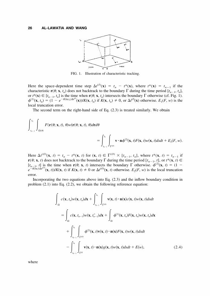
Here the space-dependent time step �t(I)(x) � tn t*(x), where t*(x) � tn1 if thecharacteristic r(�; x, tn) does not backtrack to the boundary � during the time period [tn1, tn],or t*(x) � [tn1, tn] is the time when r(�; x, tn) intersects the boundary � otherwise (cf. Fig. 1).(1)(x, tn) � (1 eK(x,tn)�t(I)

(x))/K(x, tn) if K(x, tn) � 0, or �t(I)(x) otherwise. E1(F, w) is thelocal truncation error.

The second term on the right-hand side of Eq. (2.3) is treated similarly. We obtain

�tn1

tn ��

F�r��; x, t�, ��w�r��; x, t�, ��drd�

� �tn1

tn ��O�

v � n�2��x, t�F�x, t�w�x, t�dsdt � E2�F, w�.

Here �t(O)(x, t) � tn t*(x, t) for (x, t) � �(O) � [tn1, tn], where t*(x, t) � tn1 ifr(�; x, t) does not backtrack to the boundary � during the time period [tn1, t], or t*(x, t) �[tn1, t] is the time when r(�; x, t) intersects the boundary � otherwise. (2)(x, t) � (1 eK(x,t)�t(O)

(x, t))/K(x, t) if K(x, t) � 0 or �t(O)(x, t) otherwise. E2(F, w) is the local truncationerror.

Incorporating the two equations above into Eq. (2.3) and the inflow boundary condition inproblem (2.1) into Eq. (2.2), we obtain the following reference equation:

��


tn ��O�

v�x, t� � n�x�c�x, t�w�x, t�dsdt

� ��

c�x, tn1�w�x, tn1� �dx � �

�

�1��x, tn�F�x, tn�w�x, tn�dx

� �tn1

tn ��O�

�2��x, t�v�x, t� � n�x�F�x, t�w�x, t�dsdt

� �tn1

tn ��I�

v�x, t� � n�x�g�x, t�w�x, t�dsdt � E�w�, (2.4)

where

FIG. 1. Illustration of characteristic tracking.


E�w� � �tn1

tn ��

c�x, t��wt�x, t� � v�x, t� � �w�x, t� � K�x, t�w�x, t��dxdt � E1�F, w� � E2�F, w�.

C. A Numerical Scheme

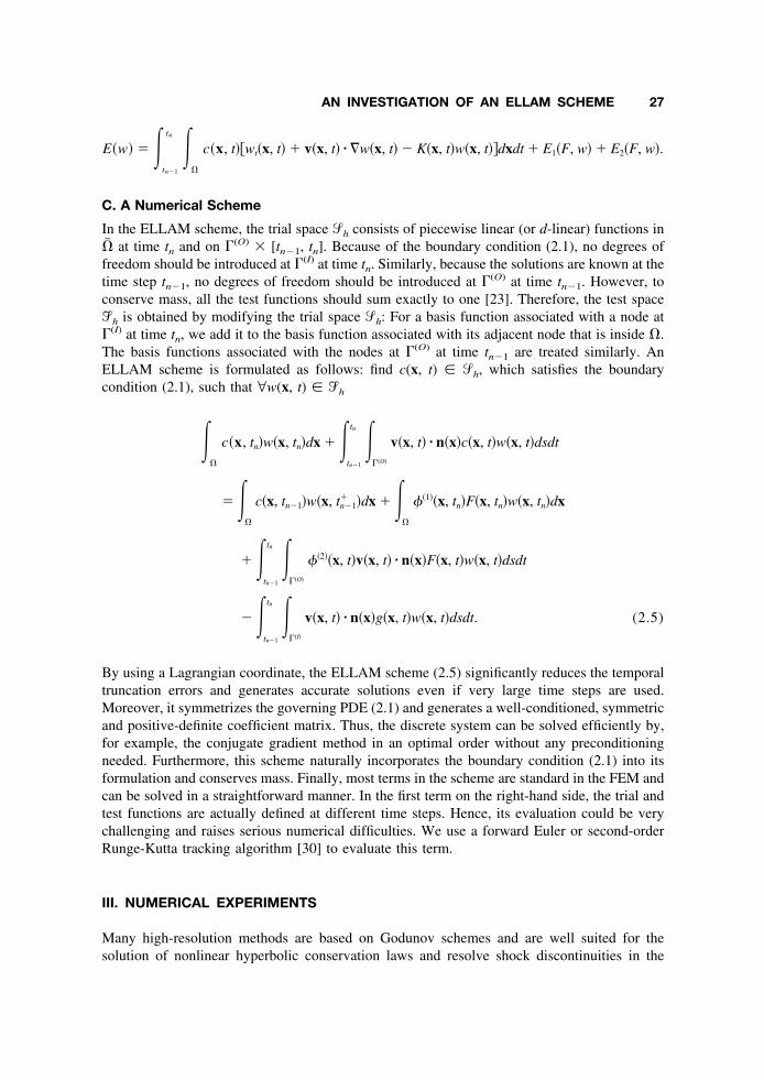
In the ELLAM scheme, the trial space �h consists of piecewise linear (or d-linear) functions in�� at time tn and on �(O) � [tn1, tn]. Because of the boundary condition (2.1), no degrees offreedom should be introduced at �(I) at time tn. Similarly, because the solutions are known at thetime step tn1, no degrees of freedom should be introduced at �(O) at time tn1. However, toconserve mass, all the test functions should sum exactly to one [23]. Therefore, the test space�� h is obtained by modifying the trial space �h: For a basis function associated with a node at�(I) at time tn, we add it to the basis function associated with its adjacent node that is inside �.The basis functions associated with the nodes at �(O) at time tn1 are treated similarly. AnELLAM scheme is formulated as follows: find c(x, t) � �h, which satisfies the boundarycondition (2.1), such that @w(x, t) � �� h

��


tn ��O�

v�x, t� � n�x�c�x, t�w�x, t�dsdt

� ��

c�x, tn1�w�x, tn1� �dx � �

�

�1��x, tn�F�x, tn�w�x, tn�dx

� �tn1

tn ��O�

�2��x, t�v�x, t� � n�x�F�x, t�w�x, t�dsdt

� �tn1

tn ��I�

v�x, t� � n�x�g�x, t�w�x, t�dsdt. (2.5)

By using a Lagrangian coordinate, the ELLAM scheme (2.5) significantly reduces the temporaltruncation errors and generates accurate solutions even if very large time steps are used.Moreover, it symmetrizes the governing PDE (2.1) and generates a well-conditioned, symmetricand positive-definite coefficient matrix. Thus, the discrete system can be solved efficiently by,for example, the conjugate gradient method in an optimal order without any preconditioningneeded. Furthermore, this scheme naturally incorporates the boundary condition (2.1) into itsformulation and conserves mass. Finally, most terms in the scheme are standard in the FEM andcan be solved in a straightforward manner. In the first term on the right-hand side, the trial andtest functions are actually defined at different time steps. Hence, its evaluation could be verychallenging and raises serious numerical difficulties. We use a forward Euler or second-orderRunge-Kutta tracking algorithm [30] to evaluate this term.

III. NUMERICAL EXPERIMENTS

Many high-resolution methods are based on Godunov schemes and are well suited for thesolution of nonlinear hyperbolic conservation laws and resolve shock discontinuities in the


solutions without excessive smearing or spurious oscillations. In this section we carry outnumerical experiments to investigate the performance of the ELLAM scheme and several highresolution methods for linear advection-reaction Eq. (2.1). This list includes the MUSCLscheme, the minmod scheme, the FCT method, and the third- and fourth-order ENO and WENOschemes [12–14, 16, 26–29]. These methods are developed as an improvement over traditionalfixed-stencil high-order FD interpolations, which are known to be oscillatory in nature espe-cially near discontinuities of the solutions. The resulting oscillations do not decay as the meshis refined and lead to further instabilities in the solution.

A. Test Problem

The test problem is an incompressible flow in a two-dimensional homogeneous medium, wherethe analytical solution is known. This example entails the rotation of the initial configuration andis a widely used to test for a variety of numerical artifacts including deformation, nonphysicaloscillations, numerical diffusion, numerical stability, and phase error. We refer readers to [31,32] for the performance of the ELLAM scheme for problems with discontinuities.

In the numerical experiments, the spatial domain is � � (0.5, 0.5) � (0.5, 0.5). Arotating velocity field of v(x, y) � (4y, 4x) is used, which gives one complete rotation in thetime interval of [0, T] � [0, /2]. The initial condition c0(x) is

c0�x� � exp��x � xc�2

2�2 �, (3.1)

where xc � (xc, yc), and � are the center and standard deviations of the Gaussian pulse. Thecorresponding analytical solution for a homogeneous Eq. (2.1) is

c�x, t� � exp��x� � xc�2

2�2 � �0

t

K�r��; x� , 0�, ��d��, (3.2)

where x� � (x�, y�) � (x cos(4t) � y sin(4t), x sin(4t) � x cos(4t)), and r(�; x� , 0) � (x� cos(4� ) y� sin(4� ), x� sin(4�) � y� cos(4�)). In this experiment we assume no reaction is present, i.e.,K(x, t) � 0. Hence, the analytic solution at T � /2 is identical to the initial solution c0(x),where we select the center parameters to be xc � 0.25 and yc � 0, while we choose � �0.0447, which gives 2�2 � 0.004.

B. The ELLAM Simulation

In the numerical example run, we choose a uniform spatial mesh of h � �x � �y � 164

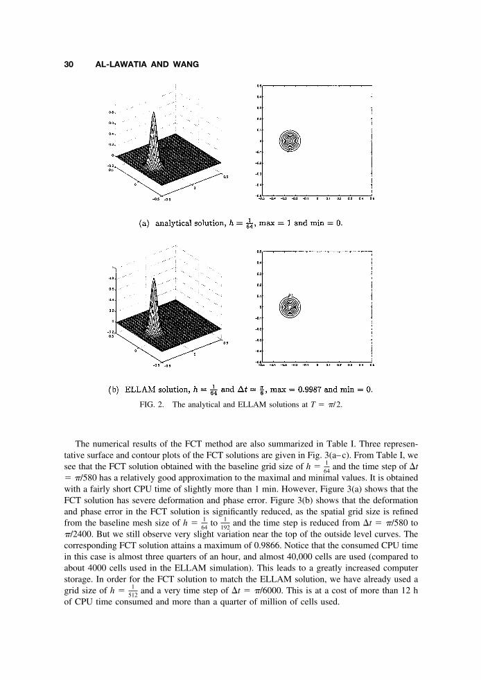
, whichis fine enough to represent the steep analytical solution. Hence this is used as the baseline meshparameter in our numerical simulations. In the ELLAM simulation, we use the same spatial gridsize and a very coarse time step of �t � /8 to solve the ELLAM scheme. Within each globaltime step �t we use a second-order Runge-Kutta method with a micro time step �tf to track thecharacteristics. In Table I we present the details of the analytical solution and the ELLAMsolution at time T � /2, including the maximum and minimum values of the solution as wellas the CPU time consumed in the simulation (measured on an SGI Workstation). In Fig. 2 wepresent the surface and contour plots of the analytical solution and the ELLAM solution. Weobserve that even with a very coarse spatial grid and a very large time step (which gives a large


Courant number of 71.25), the ELLAM solution is very accurate and maintains the profile of theexact solution with high precision without suffering from any artifacts. Furthermore, this highlyaccurate ELLAM solution is obtained with a very short CPU time of slightly more than oneminute.

C. FCT Simulation

Because all the high-resolution methods reviewed in Section 3 are explicit methods, they aresubject to the CFL condition that limits the size of the time steps allowed. Therefore, in orderto give a fair comparison, we start from the baseline spatial mesh of h � 1

64and a largest

permissible time step of �t � /580, which guarantees a Courant number of less than one, inthe numerical simulations to observe the behavior of the corresponding numerical solutions. Wethen refine the spatial grid size and observe the behavior of the solution for a variety ofdecreasing time steps that satisfies the CFL condition. We present the numerical results inTables I–V. Moreover, we present three representative surface and contour plots for eachmethod compared in Figures 3–9. The first plot (labeled (a)) in each of these figures is for thesolution generated with the baseline space mesh size of h � 1

64and a largest possible time step

of �t � /580. The third plot (labeled (c)) in each of these figures is for the solution that iscomparable to the ELLAM solution and is obtained using whatever fine spatial meshes and timesteps needed. The second plot (labeled (b)) in each of these figures gives an intermediatesolution using the spatial grids and time steps in between.

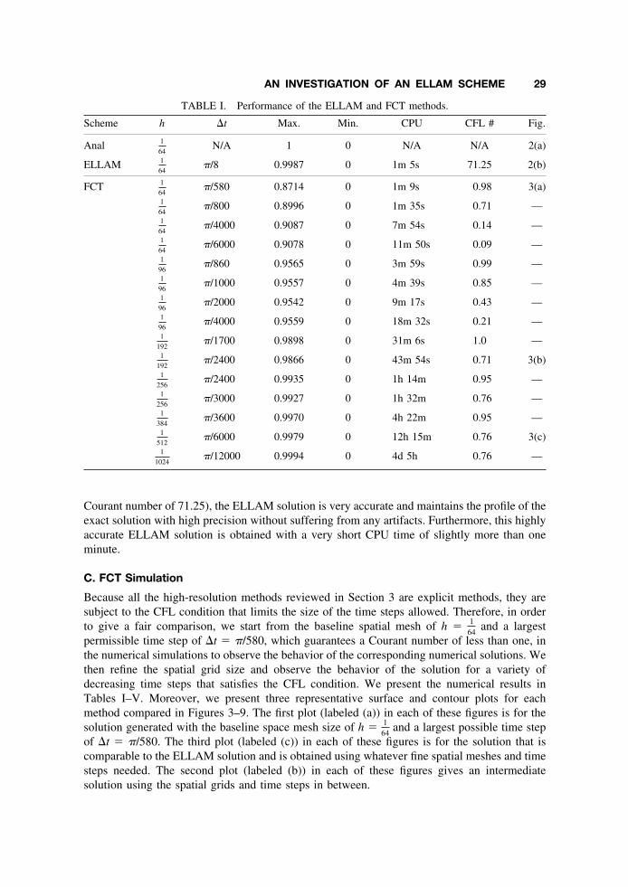
TABLE I. Performance of the ELLAM and FCT methods.

Scheme h �t Max. Min. CPU CFL # Fig.

Anal 1

64N/A 1 0 N/A N/A 2(a)

ELLAM 1

64/8 0.9987 0 1m 5s 71.25 2(b)

FCT 1

64/580 0.8714 0 1m 9s 0.98 3(a)

1

64/800 0.8996 0 1m 35s 0.71 —

1

64/4000 0.9087 0 7m 54s 0.14 —

1

64/6000 0.9078 0 11m 50s 0.09 —

1

96/860 0.9565 0 3m 59s 0.99 —

1

96/1000 0.9557 0 4m 39s 0.85 —

1

96/2000 0.9542 0 9m 17s 0.43 —

1

96/4000 0.9559 0 18m 32s 0.21 —

1

192/1700 0.9898 0 31m 6s 1.0 —

1

192/2400 0.9866 0 43m 54s 0.71 3(b)

1

256/2400 0.9935 0 1h 14m 0.95 —

1

256/3000 0.9927 0 1h 32m 0.76 —

1

384/3600 0.9970 0 4h 22m 0.95 —

1

512/6000 0.9979 0 12h 15m 0.76 3(c)

1

1024/12000 0.9994 0 4d 5h 0.76 —


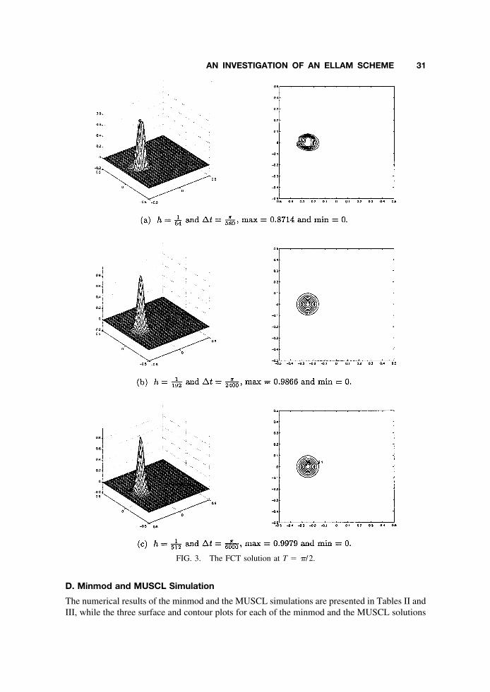
The numerical results of the FCT method are also summarized in Table I. Three represen-tative surface and contour plots of the FCT solutions are given in Fig. 3(a–c). From Table I, wesee that the FCT solution obtained with the baseline grid size of h � 1

64and the time step of �t

� /580 has a relatively good approximation to the maximal and minimal values. It is obtainedwith a fairly short CPU time of slightly more than 1 min. However, Figure 3(a) shows that theFCT solution has severe deformation and phase error. Figure 3(b) shows that the deformationand phase error in the FCT solution is significantly reduced, as the spatial grid size is refinedfrom the baseline mesh size of h � 1

64to 1

192and the time step is reduced from �t � /580 to

/2400. But we still observe very slight variation near the top of the outside level curves. Thecorresponding FCT solution attains a maximum of 0.9866. Notice that the consumed CPU timein this case is almost three quarters of an hour, and almost 40,000 cells are used (compared toabout 4000 cells used in the ELLAM simulation). This leads to a greatly increased computerstorage. In order for the FCT solution to match the ELLAM solution, we have already used agrid size of h � 1

512and a very time step of �t � /6000. This is at a cost of more than 12 h

of CPU time consumed and more than a quarter of million of cells used.

FIG. 2. The analytical and ELLAM solutions at T � /2.


D. Minmod and MUSCL Simulation

The numerical results of the minmod and the MUSCL simulations are presented in Tables II andIII, while the three surface and contour plots for each of the minmod and the MUSCL solutions

FIG. 3. The FCT solution at T � /2.


are presented in Figures 4 and 5, respectively. We see from Tables II and III and Figs. 4(a) and5(a) that with the baseline spatial mesh of h � 1

64and the time step of �t � /580, both methods

yield solutions with excessive numerical diffusion. Moreover, the solutions fail to accurately

FIG. 4. The Minmod solution at T � /2.


represent the high profile of the solution. The maximum values of the minmod solution and theMUSCL solution are 0.4223 and 0.6604, respectively. Both solutions have much less deforma-tion and phase error than the FCT solution.

FIG. 5. The MUSCL solution at T � /2.


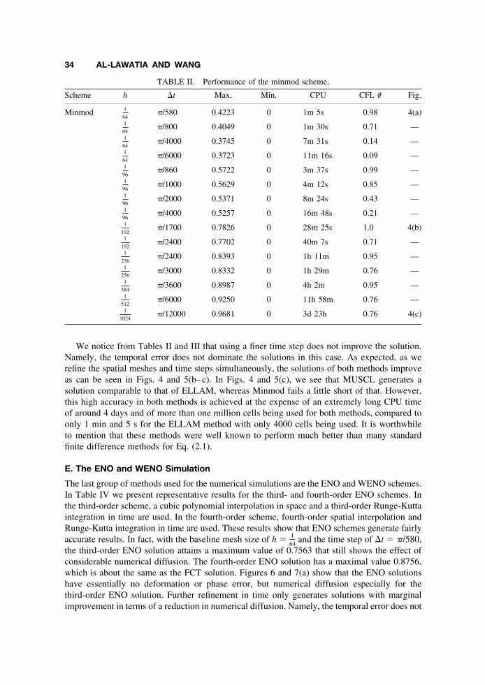
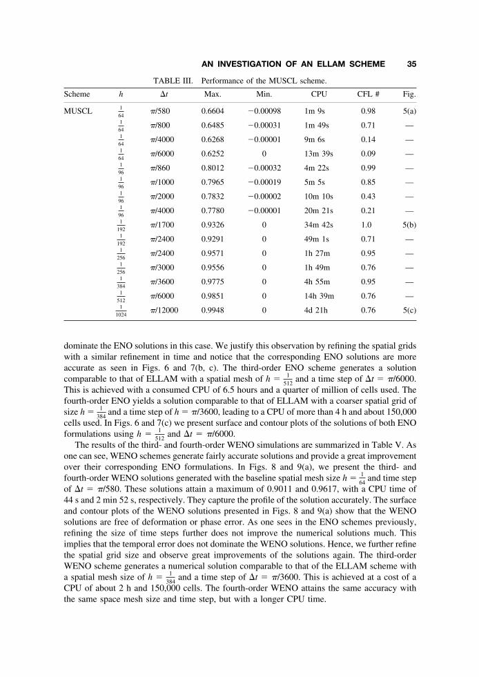
We notice from Tables II and III that using a finer time step does not improve the solution.Namely, the temporal error does not dominate the solutions in this case. As expected, as werefine the spatial meshes and time steps simultaneously, the solutions of both methods improveas can be seen in Figs. 4 and 5(b–c). In Figs. 4 and 5(c), we see that MUSCL generates asolution comparable to that of ELLAM, whereas Minmod fails a little short of that. However,this high accuracy in both methods is achieved at the expense of an extremely long CPU timeof around 4 days and of more than one million cells being used for both methods, compared toonly 1 min and 5 s for the ELLAM method with only 4000 cells being used. It is worthwhileto mention that these methods were well known to perform much better than many standardfinite difference methods for Eq. (2.1).

E. The ENO and WENO Simulation

The last group of methods used for the numerical simulations are the ENO and WENO schemes.In Table IV we present representative results for the third- and fourth-order ENO schemes. Inthe third-order scheme, a cubic polynomial interpolation in space and a third-order Runge-Kuttaintegration in time are used. In the fourth-order scheme, fourth-order spatial interpolation andRunge-Kutta integration in time are used. These results show that ENO schemes generate fairlyaccurate results. In fact, with the baseline mesh size of h � 1

64and the time step of �t � /580,

the third-order ENO solution attains a maximum value of 0.7563 that still shows the effect ofconsiderable numerical diffusion. The fourth-order ENO solution has a maximal value 0.8756,which is about the same as the FCT solution. Figures 6 and 7(a) show that the ENO solutionshave essentially no deformation or phase error, but numerical diffusion especially for thethird-order ENO solution. Further refinement in time only generates solutions with marginalimprovement in terms of a reduction in numerical diffusion. Namely, the temporal error does not

TABLE II. Performance of the minmod scheme.


Minmod 1

64/580 0.4223 0 1m 5s 0.98 4(a)

1

64/800 0.4049 0 1m 30s 0.71 —

1

64/4000 0.3745 0 7m 31s 0.14 —

1

64/6000 0.3723 0 11m 16s 0.09 —

1

96/860 0.5722 0 3m 37s 0.99 —

1

96/1000 0.5629 0 4m 12s 0.85 —

1

96/2000 0.5371 0 8m 24s 0.43 —

1

96/4000 0.5257 0 16m 48s 0.21 —

1

192/1700 0.7826 0 28m 25s 1.0 4(b)

1

192/2400 0.7702 0 40m 7s 0.71 —

1

256/2400 0.8393 0 1h 11m 0.95 —

1

256/3000 0.8332 0 1h 29m 0.76 —

1

384/3600 0.8987 0 4h 2m 0.95 —

1

512/6000 0.9250 0 11h 58m 0.76 —

1

1024/12000 0.9681 0 3d 23h 0.76 4(c)


dominate the ENO solutions in this case. We justify this observation by refining the spatial gridswith a similar refinement in time and notice that the corresponding ENO solutions are moreaccurate as seen in Figs. 6 and 7(b, c). The third-order ENO scheme generates a solutioncomparable to that of ELLAM with a spatial mesh of h � 1

512and a time step of �t � /6000.

This is achieved with a consumed CPU of 6.5 hours and a quarter of million of cells used. Thefourth-order ENO yields a solution comparable to that of ELLAM with a coarser spatial grid ofsize h � 1

384and a time step of h � /3600, leading to a CPU of more than 4 h and about 150,000

cells used. In Figs. 6 and 7(c) we present surface and contour plots of the solutions of both ENOformulations using h � 1

512and �t � /6000.

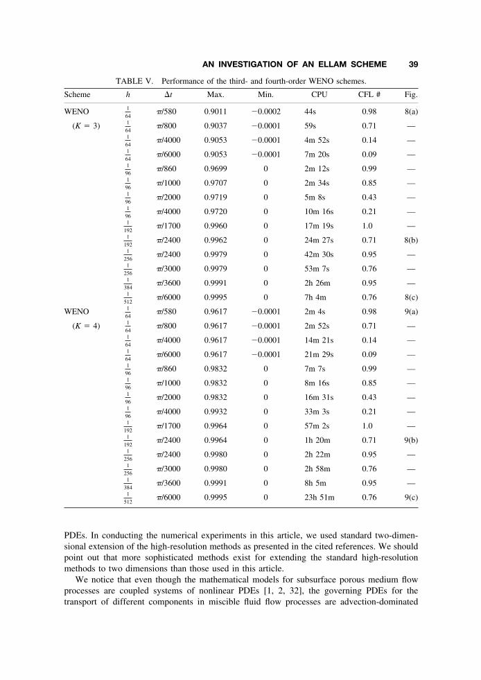
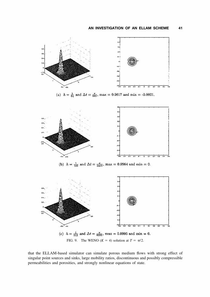
The results of the third- and fourth-order WENO simulations are summarized in Table V. Asone can see, WENO schemes generate fairly accurate solutions and provide a great improvementover their corresponding ENO formulations. In Figs. 8 and 9(a), we present the third- andfourth-order WENO solutions generated with the baseline spatial mesh size h � 1

64and time step

of �t � /580. These solutions attain a maximum of 0.9011 and 0.9617, with a CPU time of44 s and 2 min 52 s, respectively. They capture the profile of the solution accurately. The surfaceand contour plots of the WENO solutions presented in Figs. 8 and 9(a) show that the WENOsolutions are free of deformation or phase error. As one sees in the ENO schemes previously,refining the size of time steps further does not improve the numerical solutions much. Thisimplies that the temporal error does not dominate the WENO solutions. Hence, we further refinethe spatial grid size and observe great improvements of the solutions again. The third-orderWENO scheme generates a numerical solution comparable to that of the ELLAM scheme witha spatial mesh size of h � 1

384and a time step of �t � /3600. This is achieved at a cost of a

CPU of about 2 h and 150,000 cells. The fourth-order WENO attains the same accuracy withthe same space mesh size and time step, but with a longer CPU time.

TABLE III. Performance of the MUSCL scheme.


MUSCL 1

64/580 0.6604 0.00098 1m 9s 0.98 5(a)

1

64/800 0.6485 0.00031 1m 49s 0.71 —

1

64/4000 0.6268 0.00001 9m 6s 0.14 —

1

64/6000 0.6252 0 13m 39s 0.09 —

1

96/860 0.8012 0.00032 4m 22s 0.99 —

1

96/1000 0.7965 0.00019 5m 5s 0.85 —

1

96/2000 0.7832 0.00002 10m 10s 0.43 —

1

96/4000 0.7780 0.00001 20m 21s 0.21 —

1

192/1700 0.9326 0 34m 42s 1.0 5(b)

1

192/2400 0.9291 0 49m 1s 0.71 —

1

256/2400 0.9571 0 1h 27m 0.95 —

1

256/3000 0.9556 0 1h 49m 0.76 —

1

384/3600 0.9775 0 4h 55m 0.95 —

1

512/6000 0.9851 0 14h 39m 0.76 —

1

1024/12000 0.9948 0 4d 21h 0.76 5(c)


IV. SUMMARY AND DISCUSSION

In this article we carry out a preliminary investigation on an ELLAM scheme for linearadvection-reaction PDEs in multiple space dimensions by comparing its performance with manyhigh resolution methods, including the minmod scheme, the MUSCL scheme, the FCT scheme,the third- and fourth-order ENO and WENO schemes. We observe that even though very large

TABLE IV. Performance of the third- and fourth-order ENO schemes.


ENO 1

64/580 0.7563 0 43s 0.98 6(a)

(K � 3) 1

64/800 0.7572 0 56s 0.71 —

1

64/4000 0.7580 0 4m 45s 0.14 —

1

64/6000 0.7580 0 6m 59s 0.09 —

1

96/860 0.8944 0 2m 7s 0.99 —

1

96/1000 0.8948 0 2m 27s 0.85 —

1

96/2000 0.8955 0 4m 55s 0.43 —

1

96/4000 0.8956 0 9m 52s 0.21 —

1

192/1700 0.9807 0 16m 30s 1.0 —

1

192/2400 0.9808 0 23m 14s 0.71 6(b)

1

256/2400 0.9901 0 40m 12s 0.95 —

1

256/3000 0.9907 0 50m 14s 0.76 —

1

384/3600 0.9910 0 2h 17m 0.95 —

1

512/6000 0.9986 0 6h 37m 0.76 6(c)

ENO 1

64/580 0.8757 0 1m 10s 0.98 7(a)

(K � 4) 1

64/800 0.8756 0 1m 32s 0.71 —

1

64/4000 0.8756 0 7m 41s 0.14 —

1

64/6000 0.8756 0 11m 33s 0.09 —

1

96/860 0.9552 0 3m 46s 0.99 —

1

96/1000 0.9552 0 4m 22s 0.85 —

1

96/2000 0.9552 0 8m 47s 0.43 —

1

96/4000 0.9552 0 17m 20s 0.21 —

1

192/1700 0.9843 0 28m 5s 1.0 —

1

192/2400 0.9843 0 42m 21s 0.71 7(b)

1

256/2400 0.9968 0 1h 14m 0.95 —

1

256/3000 0.9981 0 1h 32m 0.76 —

1

384/3600 0.9989 0 4h 13m 0.95 —

1

512/6000 0.9993 0 12h 20m 0.76 7(c)


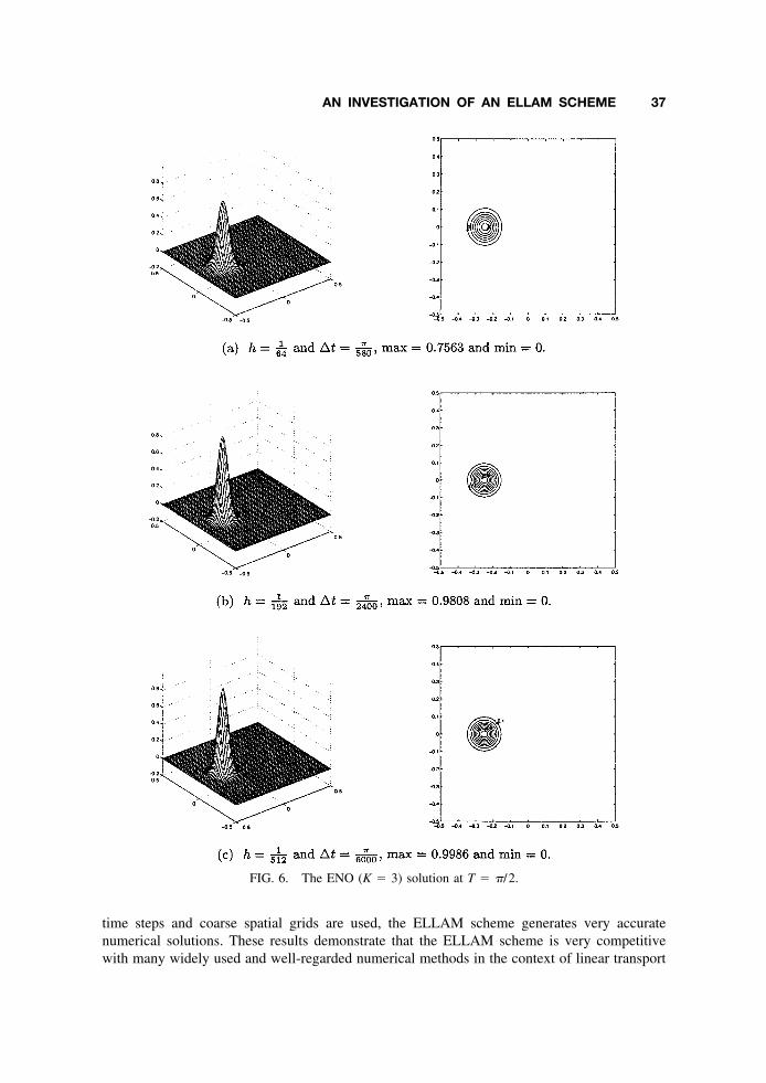
time steps and coarse spatial grids are used, the ELLAM scheme generates very accuratenumerical solutions. These results demonstrate that the ELLAM scheme is very competitivewith many widely used and well-regarded numerical methods in the context of linear transport

FIG. 6. The ENO (K � 3) solution at T � /2.


FIG. 7. The ENO (K � 4) solution at T � /2.


PDEs. In conducting the numerical experiments in this article, we used standard two-dimen-sional extension of the high-resolution methods as presented in the cited references. We shouldpoint out that more sophisticated methods exist for extending the standard high-resolutionmethods to two dimensions than those used in this article.

We notice that even though the mathematical models for subsurface porous medium flowprocesses are coupled systems of nonlinear PDEs [1, 2, 32], the governing PDEs for thetransport of different components in miscible fluid flow processes are advection-dominated

TABLE V. Performance of the third- and fourth-order WENO schemes.


WENO 1

64/580 0.9011 0.0002 44s 0.98 8(a)

(K � 3) 1

64/800 0.9037 0.0001 59s 0.71 —

1

64/4000 0.9053 0.0001 4m 52s 0.14 —

1

64/6000 0.9053 0.0001 7m 20s 0.09 —

1

96/860 0.9699 0 2m 12s 0.99 —

1

96/1000 0.9707 0 2m 34s 0.85 —

1

96/2000 0.9719 0 5m 8s 0.43 —

1

96/4000 0.9720 0 10m 16s 0.21 —

1

192/1700 0.9960 0 17m 19s 1.0 —

1

192/2400 0.9962 0 24m 27s 0.71 8(b)

1

256/2400 0.9979 0 42m 30s 0.95 —

1

256/3000 0.9979 0 53m 7s 0.76 —

1

384/3600 0.9991 0 2h 26m 0.95 —

1

512/6000 0.9995 0 7h 4m 0.76 8(c)

WENO 1

64/580 0.9617 0.0001 2m 4s 0.98 9(a)

(K � 4) 1

64/800 0.9617 0.0001 2m 52s 0.71 —

1

64/4000 0.9617 0.0001 14m 21s 0.14 —

1

64/6000 0.9617 0.0001 21m 29s 0.09 —

1

96/860 0.9832 0 7m 7s 0.99 —

1

96/1000 0.9832 0 8m 16s 0.85 —

1

96/2000 0.9832 0 16m 31s 0.43 —

1

96/4000 0.9932 0 33m 3s 0.21 —

1

192/1700 0.9964 0 57m 2s 1.0 —

1

192/2400 0.9964 0 1h 20m 0.71 9(b)

1

256/2400 0.9980 0 2h 22m 0.95 —

1

256/3000 0.9980 0 2h 58m 0.76 —

1

384/3600 0.9991 0 8h 5m 0.95 —

1

512/6000 0.9995 0 23h 51m 0.76 9(c)


PDEs that are weakly nonlinear in terms of the concerned concentrations. Thus, our investiga-tion in this article suggests and justifies the development of ELLAM-based simulators for thefully coupled system for porous medium flows [3]. The computational experiments in [3] show

FIG. 8. The WENO (K � 3) solution at T � /2.


that the ELLAM-based simulator can simulate porous medium flows with strong effect ofsingular point sources and sinks, large mobility ratios, discontinuous and possibly compressiblepermeabilities and porosities, and strongly nonlinear equations of state.

FIG. 9. The WENO (K � 4) solution at T � /2.


In immiscible subsurface fluid flow processes, the saturation PDEs typically have S-shapednonlinear flux functions. Hence, characteristic methods cannot be applied directly. Operator-splitting techniques were previously proposed (e.g., in the context of MMOC) to overcome thisdifficulty [33]. This would split the fractional flow function f into an advective concave hull �fof f, which is linear in what would be the shock region, and a residual antidiffusive part. Acharacteristic tracking is applied to �f to yield the same entropy solution as the original PDE. Theresidual antidiffusive advection term is treated by upstream weighting in space to incorporate theself-sharpening effect in the full solution. On the other hand, high-resolution methods are wellsuited for nonlinear hyperbolic conservation laws and resolve shock discontinuities and complexsolution structures. They have been successfully applied in aerodynamics and other applicationsand are very competitive for immiscible flow problems. Some hybrid mixtures of characteristicand high-resolution methods would be a potentially very competitive numerical simulationtechnique for multiphase-multicomponent or compositional models and remain to be developed.

The authors also thank the referees for their very helpful comments and suggestions, whichimproved the quality of this paper.

References

1. J. Bear, Hydraulics of Groundwater, McGraw-Hill, New York, 1979.

2. R. E. Ewing, editor, The mathematics of reservoir simulation, Research frontiers in applied mathe-matics, 1, SIAM, Philadelphia, 1984.

3. H. Wang, D. Liang, R. E. Ewing, S. L. Lyons, and G. Qin, An approximation to miscible fluid flowsin porous media with point sources and sinks by an Eulerian-Lagrangian localized adjoint method andmixed finite element methods, SIAM J Sci Comput 22 (2000), 561–581.

4. J. W. Barrett and K. W. Morton, Approximate symmetrization and Petrov-Galerkin methods fordiffusion-convection problems, Comp Meth Appl Mech Eng 45 (1984), 97–122.

5. M. A. Celia, I. Herrera, E. T. Bouloutas, and J. S. Kindred, A new numerical approach for theadvective-diffusive transport equation, Num Meth PDEs 5 (1989), 203–226.

6. I. Christie, D. F. Griffiths, A. R. Mitchell, and O. C. Zienkiewicz, Finite element methods for secondorder differential equations with significant first derivatives, Int J Num Eng 10 (1976), 1389–1396.

7. E. T. Bouloutas and M. A. Celia, An improved cubic Petrov-Galerkin method for simulation oftransient advection-diffusion processes in rectangularly decomposable domains, Comp Meth ApplMech Eng 91 (1991), 289–308.

8. R. A. Cox and T. Nishikawa, A new total variation diminishing scheme for the solution of advective-dominant solute transport, Water Resources Res 27 (1991), 2645–2654.

9. J. J. Westerink and D. Shea, Consistent higher degree Petrov-Galerkin methods for the solution of thetransient convection-diffusion equation, Int J Num Meth Eng 28 (1989), 1077–1101.

10. T. J. R. Hughes and A. N. Brooks, A multidimensional upwinding scheme with no cross-winddiffusion, Hughes, editor, Finite element methods for convection dominated flows, Vol. 34, ASME,New York, 1979.

11. C. Johnson, A. Szepessy, and P. Hansbo, On the convergence of shock-capturing streamline diffusionfinite element methods for hyperbolic conservation laws, Math Comp 54 (1990), 107–129.

12. P. Colella, A direct Eulerian MUSCL scheme for gas dynamics, SIAM J Sci Stat Comp 6 (1985),104–117.

13. A. Harten, B. Engquist, S. Osher, and S. Chakravarthy, Uniformly high order accurate essentiallynonoscillatory schemes, III, J Comp Phys 71 (1987), 231–241.


14. C. Shu and S. Osher, Efficient implementation of essentially non-oscillatory shock capturing schemes,J Comput Phys 77 (1988), 439–471.

15. P. K. Sweby, High resolution schemes using flux limiters for hyperbolic conservation laws, SIAM JNumer Anal 28 (1991), 891–906.

16. B. van Leer, On the relation between the upwind-differencing schemes of Godunov, Engquist-Osher,and Roe, SIAM J Sci Stat Comp 5 (1984), 1–20.

17. S. K. Godunov, A difference scheme for numerical computation of discontinuous solutions of fluiddynamics, Mat Sb 47 (1959), 271–306.

18. R. Courant, E. Isaacson, and M. Rees, On the solution of nonlinear hyperbolic differential equationsby finite differences, Comm Pure Appl Math 5 (1952), 243–255.

19. J. Douglas, Jr., and T. F. Russell, Numerical methods for convection-dominated diffusion problemsbased on combining the method of characteristics with finite element or finite difference procedures,SIAM J Num Anal 19 (1982), 871–885.

20. A. O. Garder, D. W. Peaceman, and A. L. Pozzi, Numerical calculations of multidimensional miscibledisplacement by the method of characteristics, Soc Pet Eng J 4 (1964), 26–36.

21. O. Pironneau, On the transport-diffusion algorithm and its application to the Navier-Stokes equations,Num Math 38 (1982), 309–332.

22. E. Varoglu and W. D. L. Finn, Finite elements incorporating characteristics for one-dimensionaldiffusion-convection equation, J Comp Phys 34 (1980), 371–389.

23. M. A. Celia, T. F. Russell, I. Herrera, and R. E. Ewing, An Eulerian-Lagrangian localized adjointmethod for the advection-diffusion equation, Adv Water Res 13 (1990), 187–206.

24. R. E. Ewing and H. Wang, Eulerian-Lagrangian localized adjoint methods for linear advectionequations, Computational Mechanics ’91, Springer International, New York, 1991, pp. 245–250.

25. R. E. Ewing and H. Wang, Eulerian-Lagrangian localized adjoint methods for linear advection oradvection-reaction equations and their convergence analysis, Comput Mech 12 (1993), 97–121.

26. J. P. Boris and D. L. Book, Flux-corrected transport I, SHASTA, a fluid transport algorithm that works,J Comput Phys 11 (1973), 38–69.

27. J. P. Boris and D. L. Book, Flux-corrected transport, III, Minimal-error FCT algorithms, J ComputPhys 20 (1976), 397–431.

28. X.-D. Liu, S. Osher, and T. Chan, Weighted essentially nonoscillatory schemes, J Comput Phys 115(1994), 200–212.

29. S. T. Zalesak, Fully multidimensional flux-corrected transport algorithms for fluids, J Comput Phys 31(1978), 335–362.

30. T. F. Russell and R. V. Trujillo, Eulerian-Lagrangian localized adjoint methods with variablecoefficients in multiple dimensions, Gambolati et al., editors, Computational methods in surfacehydrology, Springer-Verlag, Berlin, 1990, pp. 357–363.

31. M. Al-Lawatia, R. C. Sharpley, and H. Wang, Second-order characteristic methods for advection-diffusion equations and comparison to other schemes, Adv Water Res 22 (1999), 741–768.

32. H. Wang, R. E. Ewing, G. Qin, S. L. Lyons, M. Al-Lawatia, and S. Man, A family of Eulerian-Lagrangian localized adjoint methods for multi-dimensional advection-reaction equations, J ComputPhys 152 (1999), 120–163.

33. M. S. Espedal and R. E. Ewing, Characteristic Petrov-Galerkin sub-domain methods for two-phaseimmiscible flow, Comp Meth Appl Mech Eng 64 (1987), 113–135.


Download - A preliminary investigation on an ELLAM scheme for linear transport equations

Top Related