Farr
Fields, LC
1
A Power Wave Theory of Antennas
Everett G. Farr Farr Fields, LC
City University of Hong Kong August 26, 2014
Hong Kong
Farr
Fields, LC
2
Overview
Part 1: Some UWB Antennas We’ve Worked On
Part 2: The Power Wave Theory of Antennas

Farr
Fields, LC
3
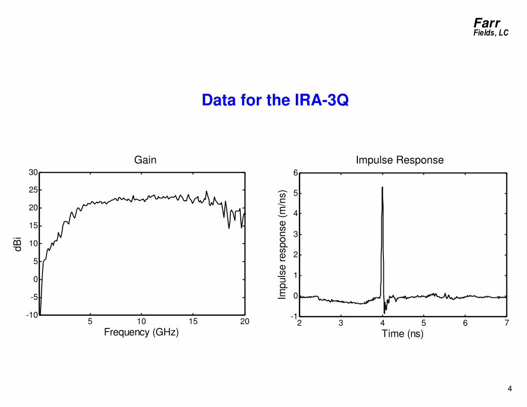
Example of UWB Antenna: IRA-3Q
• Diameter: 18 in. (46 cm)
• Radiates a Clean Impulse, with FWHM = 38 ps.
• Frequency range 250 MHz – 20 GHz.
• Excellent impedance match across entire frequency range.
Farr
Fields, LC
4
Data for the IRA-3Q
Gain Impulse Response
5 10 15 20-10
-5
0
5
10
15
20
25
30
Frequency (GHz)
dB
i
2 3 4 5 6 7-1
0
1
2
3
4
5
6
Time (ns)
Impuls
e r
esponse (
m/n
s)
Farr
Fields, LC
5
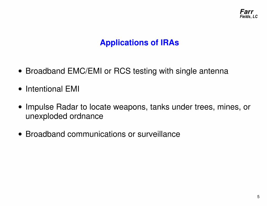
Applications of IRAs
• Broadband EMC/EMI or RCS testing with single antenna
• Intentional EMI
• Impulse Radar to locate weapons, tanks under trees, mines, or unexploded ordnance
• Broadband communications or surveillance
Farr
Fields, LC
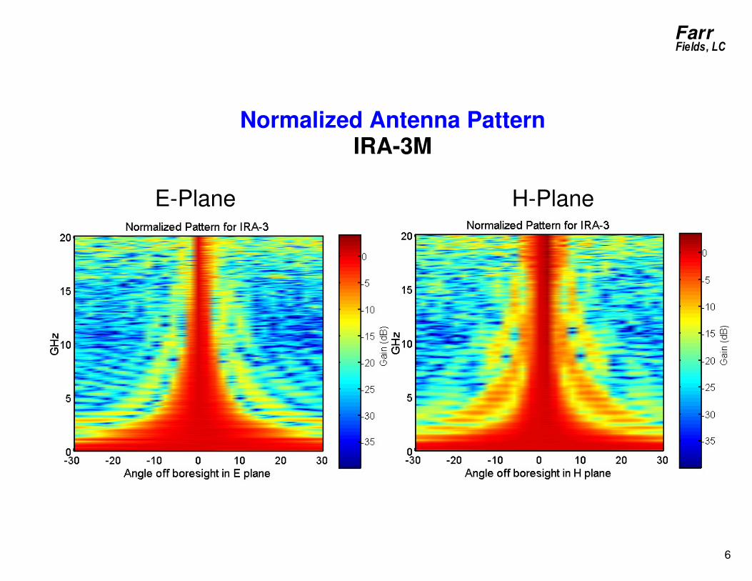
6
Normalized Antenna Pattern IRA-3M
E-Plane H-Plane

Farr
Fields, LC
7
Radome on IRA
IRA-3

Farr
Fields, LC
8
Collapsible IRA
• Compact, Lightweight, rapidly deployable design
• Metallized nylon and resistive fabric
• When collapsed: Length=81 cm, Diam=10 cm
• Suitable for broadband communications in field
• Impulse response FWHM = 70 ps
• Peak Gr = 23 dB at 4 GHz
• Useful from 150 MHz to 8 GHz

Farr
Fields, LC
9
CIRA-2 Data
Impulse Response Gain

Farr
Fields, LC
10
Para-IRA Concept
• Parachute Delivered
• Impulse Radiating Antenna
• Goal is to Illuminate 100-Meter Radius Area with a Wideband Pulse
• Parachute Allows Rapid and Flexible Deployment
Parachute
Parabolic ReflectorConducting MeshFabric
TerminatingResistor
UnzipperBalun
Battery
Feed ArmsConductiveRipstopNylon
Transmitter

Farr
Fields, LC
11
Phase I Antenna Mounted Onto Frame for Testing

Farr
Fields, LC
12
Phase I Tow Test Results
• Measure force on scale to correlate terminal velocity with weight
• Descent Rate Results: A 20 pound package falls at 58 kph

Farr
Fields, LC
13
Folded Horn Antenna
• Useful for medium bandwidth (3-5 GHz) at high power
• Could be scaled X10 to reach 300-500 MHz, and mounted onto truck.
• Nearly flat phase front in aperture

Farr
Fields, LC
14
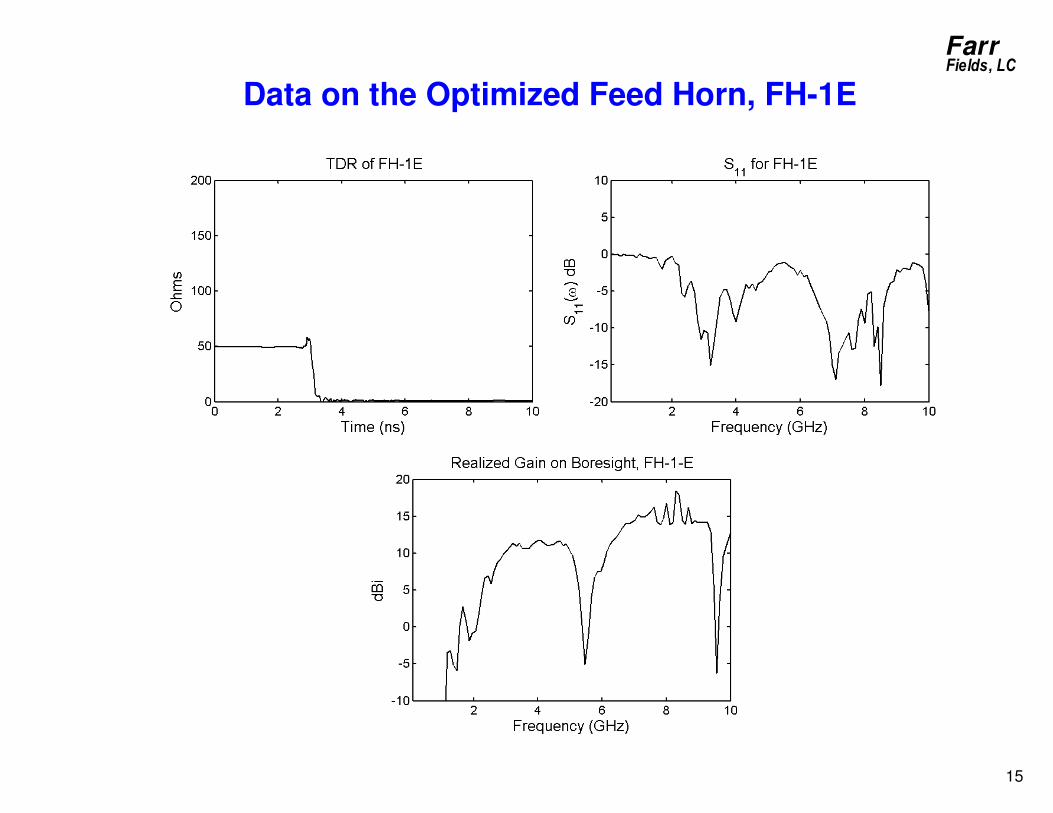
Feed Point Modifications in FH-1E
• Add dielectric disk: Simulates oil tank near feed, and shifts the
dip in S11 to lower frequency
• Add cone: to maintain 50-Ω impedance
( )2/cotln2
hoZ θπ
η=
• We needed both!
Farr
Fields, LC
15
Data on the Optimized Feed Horn, FH-1E

Farr
Fields, LC
16
Time Domain Antenna Measurement System
• With the PATAR® system one person can set up an antenna range, take and process data, then tear down and store the equipment all within 4 hours.
• Equipment fits into a shed
• No anechoic chamber needed due to time gating and temperature stability of scopes
• Bandwidth of 900 MHz to 20 GHz for arbitrary antennas
• For impulse antennas, bandwidth reaches as low as 200 MHz
• Works as well for narrowband antennas as for UWB antennas
• Introduces concept of “Personal Antenna Range”

Farr
Fields, LC
17
Measurement Setup
PSPL 4015D Step Generator
Tektronix TDS 8300 Series Digital Sampling
Oscilloscope with 80E04 Sampling Head
and 2m Extender
Remote Pulser Head
Antenna Under Test
Trigger Line
Received Signal
AZ–EL Positioner
Computer Controller
Transmit Antenna
RS232 Link
Ethernet Link
Farr
Fields, LC
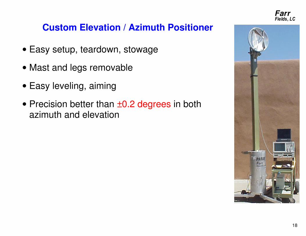
18
Custom Elevation / Azimuth Positioner
• Easy setup, teardown, stowage
• Mast and legs removable
• Easy leveling, aiming
• Precision better than ±0.2 degrees in both azimuth and elevation

Farr
Fields, LC
19
Source End of Range
Includes Pulser, mounting Bracket, and
TEM sensor on fixed tripod

Farr
Fields, LC
20
Parameters Calculated
Impulse Response Return Loss (S11)
Gain, Realized Gain Antenna Pattern
Farr
Fields, LC
21
Part 2: The Power Wave Theory of Antennas

Farr
Fields, LC
22
The Antenna Equation and the Generalized Antenna Scattering Matrix (GASM)
Dominant Polarization on Boresight
r
o
rad
rad
eZ
Er γ
Υ
2
~
~=
1
~~
o
recrec
V
ΖΠ =
1
~~
o
srcsrc
V
ΖΠ =
2
~~
o
incinc
Z
E=Σ
1oZ
inZ~
2oZ
Γ=
inc
src
rad
rec
vhs
h
Σ
Π
πΥ
Π~
~
~)2/(
~
~~
~
~
l
GASM completely specifies response of any antenna, including those with waveguide feeds.
Farr
Fields, LC
23
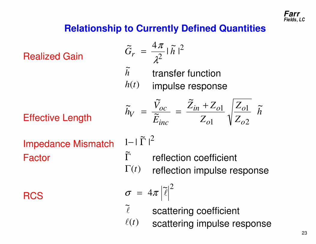
Relationship to Currently Defined Quantities
Realized Gain 2
2|
~|
4~hGr
λ
π=
h~
transfer function
)(th impulse response
Effective Length h
Z
Z
Z
ZZ
E
Vh
o
o
o
oin
inc
ocV
~~
~
~~
2
1
1
1+==
Impedance Mismatch 2|
~|1 Γ−
Factor Γ~
reflection coefficient
)(tΓ reflection impulse response
RCS 2~
4 lπσ =
l~
scattering coefficient
)(tl scattering impulse response

Farr
Fields, LC
24
New Definitions and Symbols
waveintensity radiation radiated
~~
vedensity waflux power incident
~~
power wave received
~~
power wave source
~~
2
2
1
1
==
==
==
==
r
o
radrad
o
incinc
o
recrec
o
srcsrc
eZ
Er
Z
E
V
V
γΥ
Σ
ΖΠ
ΖΠ
Π, Σ, and Υ are Greek for P, S, and U, which are the commonly used symbols for power, power flux density, and radiation intensity.

Farr
Fields, LC
25
Relationships between Power Expressions and
Power Wave Expressions
Power Power Wave
( )( ) 2*
2*
~~~Re
21~
~~~Re
21~
recrecrecrec
srcsrcsrcsrc
IVP
IVP
Π
Π
==
==
Power Flux Density Power Flux Density Wave
2* ~~~
Re2
1~incincincinc AdHES Σ=•
×= ∫∫
rrr
Radiation Intensity Radiation Intensity Wave
22* ~
ˆ~~
Re2
1~radradradrad rrHEU Υ=•
×=
rr
Power waves add phase to well-known power expressions.

Farr
Fields, LC
26
Antenna Equation and GASM in the Time Domain
• Antenna equation and GASM in the time domain
•
′
Γ=
)(
)(*
)(2/)(
)()(
)(
)(
t
t
tvth
tht
t
t
inc
src
rad
rec
Σ
Π
πΥ
Π
l
where “ ' ” indicates a time derivative and the “•* ” operator is a
matrix-product convolution operator, defined as
∗+∗
∗+∗=
∗
•
)()()()(
)()()()(
)(
)(
)()(
)()(
222121
212111
2
1
2221
1211
tatstats
tatstats
ta
ta
tsts
tsts

Farr
Fields, LC
27
Antenna Equation for Two Polarizations and Arbitrary Angles
Frequency Domain
′′′′
′′′′
′′′′Γ
=
′′
′′
′′
)','(~
)','(~
~
),,,(~
),,,(~
)2/(),(~
),,,(~
),,,(~
)2/(),(~
),(~
),(~~
),,,(~
),,,(~
),(~
,
,
,
,
φθΣ
φθΣ
Π
φθφθφθφθπφθ
φθφθφθφθπφθ
φθφθ
φθφθΥ
φθφθΥ
φθΠ
φ
θ
φφφθφ
θφθθθ
φθ
φ
θ
inc
inc
src
rad
rad
rec
vhs
vhs
hh
ll
ll
),( φθ ′′ source coordinates ),( φθ observation coordinates
Time Domain
′′
′′∗
′′′′′
′′′′′
′′′′Γ
=
′′
′′
′′
•
),,(
),,(
)(
),,,,(),,,,()2/(),,(
),,,,(),,,,()2/(),,(
),,(),,()(
),,,,(
),,,,(
),,(
,
,
,
,
t
t
t
ttvth
ttvth
ththt
t
t
t
inc
inc
src
rad
rad
rec
φθΣ
φθΣ
Π
φθφθφθφθπφθ
φθφθφθφθπφθ
φθφθ
φθφθΥ
φθφθΥ
φθΠ
φ
θ
φφφθφ
θφθθθ
φθ
φ
θ
ll
ll
More Compact Frequency Domain Expression
Γ=
inc
src
rad
rec
vhj
h
Σ
Π
πωΥ
Π~
~
~)2/(
~
~~~
~ T
r
ltr
r
r

Farr
Fields, LC
28
Signal Flow Graphs
Dominant polarization, on boresight
radΥ
~
recΠ~
srcΠ~
incΣ~
Γ~
h~ l
~)2/(
~vhs π 1
1
1
1
Both polarizations, arbitrary angles, vectorized 2-port version
radΥ~r
recΠ~
srcΠ~
incΣ~r
Γ~
T~hr
lr~
)2/(~
vhs πr
1
1
1
1

Farr
Fields, LC
29
Signal Flow Graphs (cont’d)
Both polarizations, arbitrary angles, scalar 3-port version
recΠ~
srcΠ~
Γ~
θh~
θθl~
)2/(~
vhs πθ
1
1
rad,~
θΥ
inc,~
θΣ
1
1
φφl~
rad,~
φΥ
inc,~
φΣ
1
1
φθl~
)2/(~
vhs πφ
φh~
θφl~

Farr
Fields, LC
30
Solve Arbitrary Source with Signal Flow Graph
radΥ
~
recΠ~
srcΠ~
Γ~
)2/(~
vhs π
srcΓ~
1
1
1~
~~
osrc
osrcsrc
ZZ
ZZ
+
−=Γ
Dominant polarization, on boresight
srcsrc
radv
hsΠ
πΥ
~
2
~
~~1
1~
ΓΓ−=
Both polarizations, arbitrary angles
srcsrc
radv
hsΠ
π
φθφθΥ
~
2
),(~
~~1
1),(
~r
r
ΓΓ−=
Farr
Fields, LC
31
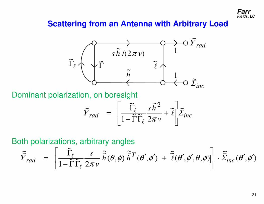
Scattering from an Antenna with Arbitrary Load
radΥ
~
incΣ~
Γ~
h~ l
~)2/(
~vhs π 1
1
lΓ~
Dominant polarization, on boresight
incradv
hsΣ
πΥ
~~
2
~
~~1
~~
2
+
ΓΓ−
Γ= l
l
l
Both polarizations, arbitrary angles
),(~
),,,(~
),(~
),(~
2~~
1
~~φθΣφθφθφθφθ
πΥ ′′⋅
′′+′′
ΓΓ−
Γ= inc
Trad hh
v
s rl
trrr
l
l
Farr
Fields, LC
32
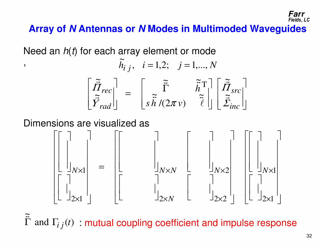
Array of N Antennas or N Modes in Multimoded Waveguides
Need an h(t) for each array element or mode ,
Γ=
inc
src
rad
rec
vhs
h
Σ
Π
πΥ
Π~
~
~)2/(
~
~~
~
~T
r
r
ltt
tt
r
r
Dimensions are visualized as
=
×
×
××
××
×
×
12
1
222
2
12
1 N
N
NNNN
: mutual coupling coefficient and impulse response
Njih ji ,...,1;2,1,~
==
)(and~
tjiΓΓt

Farr
Fields, LC
33
Proving the Relationship between Transmission and Reception Terms
• Relate power wave expressions to open/short circuit forms using circuit theory.
• Treat two antennas in far field as reciprocal two-port network
2221
1211~~
~~
ZZ
ZZ
2221
1211~~
~~
YY
YY
Port 1 Port 2 Antenna 1 Antenna 2
• Assume Antenna 2 is an electrically small electric dipole, whose open/short circuit characteristics are fully known.

Farr
Fields, LC
34
Impulse Response Example
IRA-3Q
Impulse Response Transfer Function
2 3 4 5 6 7
-1
0
1
2
3
4
5
6
Time (ns)
Impuls
e r
esponse (
m/n
s)
10-1
100
101
10-2
10-1
100
Frequency (GHz)
Tra
nsfe
r fu
nction (
m)

Farr
Fields, LC
35
Review of Waveform Norms (For transient antenna patterns)
Three necessary conditions of norms
)inequality triangle()()()()(
linearity)()()(
otherwise
0)( iff
0
0)(
tgtftgtf
tftf
tftf
+≤+
=
≡
>
=
αα
Commonly used: p–norms
)(sup)(,)()(
/1
tftfdttftft
p
p
p=
=
∞
∞
∞−∫

Farr
Fields, LC
36
Transient Antenna Pattern
• Can consider single polarization or total magnitude
22),,(),,(),,( ththth φθφθφθ φθ +=
r
• Express transient patterns in terms of norms of time domain waveforms
),0,0(
),,(),(
),0,0(
),,(),(,
),0,0(
),,(),(
th
th
th
th
th
th
t r
rφθ
φθ
φθφθ
φθφθ
φ
φφ
θ
θθ
=
==
P
PP
• Normalization to boresight is optional

Farr
Fields, LC
37
Radiation from or Coupling into a Complex System
• Complex system looks like a poor antenna
• Antenna parameters should be used o Same in TX and RX o Works in both frequency and time domains

Farr
Fields, LC
38
Conclusion: Effects on Standards
None of the terms in the Antenna Equation have been defined
Γ=
inc
src
rad
rec
vhs
h
Σ
Π
πΥ
Π~
~
~)2/(
~
~~
~
~
l
Closest is scalar versions:
Impedance mismatch factor, 2|
~|1 Γ− , instead of Γ
~
Realized gain, rG , instead of h~
RCS, σ , instead of l~
We need to complexify the standards to get to the time domain!

Farr
Fields, LC
39
Everett Farr +1(505)410-7722
[email protected] www.farr-research.com
This paper is based on
Sensor and Simulation Note 564, Revision 3 Available at our web site
Soon to appear in FERMAT! We welcome your online comments!


