
A New Voltage Stability-Constrained Optimal Power
Flow Model: Sufficient Condition, SOCP
Representation, and Relaxation
Bai Cui ∗, Xu Andy Sun †
May 31, 2017
Abstract
A simple characterization of the solvability of power flow equations is of great im-
portance in the monitoring, control, and protection of power systems. In this paper, we
introduce a sufficient condition for power flow Jacobian nonsingularity. We show that
this condition is second-order conic representable when load powers are fixed. Through
the incorporation of the sufficient condition, we propose a voltage stability-constrained
optimal power flow (VSC-OPF) formulation as a second-order cone program (SOCP).
An approximate model is introduced to improve the scalability of the formulation to
larger systems. Extensive computation results on Matpower and NESTA instances
confirm the effectiveness and efficiency of the formulation.
1 Introduction
Power flow equations are ubiquitous in power system analysis. It is shown in [1] that the
singularity of power flow Jacobian is closely related to the loss of steady-state stability. In
the paper, we consider the steady-state voltage stability problem as a power flow solvability
problem. Reliable numerical tools to calculate the distance to power flow stability boundary
are available [2, 3, 4]. However, these tools provide no explicit conditions certifying power flow
feasibility, which makes the incorporation of voltage stability conditions in other problems a
challenge.
∗B. Cui is with the School of Electrical and Computer Engineering, Georgia Institute of Technology, 765Ferst Drive, NW Atlanta, Georgia 30332-0205 (e-mail: [email protected]).†X. A. Sun is with the School of Industrial and Systems Engineering, Georgia Institute of Technology,
765 Ferst Drive, NW Atlanta, Georgia 30332-0205 (e-mail: [email protected]).
1

There has been a resurgence in recent years in the search for explicit conditions quan-
tifying the feasibility of power flow equations along the lines of Wu [5] and Ilic [6]. In [7],
a sufficient condition for existence and uniqueness of high-voltage solution in distribution
system is obtained using fixed-point argument, which is extended in [8]. Similar techniques
have subsequently been applied to yield stronger results in [9] and [10]. Conditions on solu-
tion existence and uniqueness in lossless system with PV buses are given in [11, 12]. These
methods are to be contrasted with heuristic conditions based on system equivalence [13, 14].
To avoid system instability, security constraints such as voltage magnitude limits and
line flow limits are enforced in normal system operation. However, high penetrations of dis-
tributed generators (DGs) and extensive deployment of reactive power compensation devices
are able to provide support to hold up voltages within operational bounds even when system
stability margin is low. Therefore, the effectiveness of the security constraints in safeguard-
ing system stability may be diminished in modern power systems. Another motivation for
the inclusion of steady-state stability limit in an optimal power flow (OPF) formulation is
the increasing trend to operate power systems ever closer to their operational limits due
to increased demand and competitive electricity market. Without stability constraints, the
robustness of the OPF solution against voltage instability is not ensured. Voltage stability
constraint in an OPF setting can be rigorously represented using the minimum singular value
(MSV) of the power flow Jacobian as in [15, 16, 17]. However, the computational cost of
this method is high. To achieve a better trade-off between accuracy and efficiency, some
conditions quantifying system stress level have been used in voltage stability-related OPF
problems that are either heuristic [18, 19], or based on DC [20] or reactive power flow model
[21].
We give a new and simplified proof for a sufficient condition for power flow Jacobian non-
singularity that we proposed recently in [22]. The condition can be seen as a generalization
to the heuristic condition proposed in [23]. We then formulate a voltage stability-constrained
OPF (VSC-OPF) problem in which the voltage stability margin is quantified by the condi-
tion. We show that when load powers are fixed, this voltage stability condition describes
a second-order conic representable set in a transformed voltage space. Thus second-order
cone program (SOCP) reformulation can naturally incorporate the condition. Notice that
the formulation does not require the DC or decoupled power flow assumptions. To improve
computation time, we sparsify the dense stability constraints while preserving very high
accuracy.
The rest of the paper is organized as follows. Section 2 provides background on power
system modeling. The sufficient condition for power flow Jacobian nonsingularity is intro-
duced in Section 3. We discuss the VSC-OPF formulation, its convex reformulation, and
2

sparse approximation in Section 4. Section 5 presents results of extensive computational
experiments. Concluding remarks are given in Section 6.
2 Background
2.1 Notations
The cardinality of a set or the absolute value of a (possibly) complex number is denoted by |·|.i =√−1 is the imaginary unit. R and C are the set of real and complex numbers, respectively.
For vector x ∈ Cn, ‖x‖p denotes the p-norm of x where p ≥ 1 and diag(x) ∈ Cn×n is the
associated diagonal matrix. The n-dimensional identity matrix is denoted by In. 0n×m
denotes an n×m matrix of all 0’s. For A ∈ Cn×n, A−1 is the inverse of A. For B ∈ Cm×n,
BT , BH are respectively the transpose and conjugate transpose of B, and B∗ is the matrix
with complex conjugate entries. The real and imaginary parts of B are denoted as ReB and
ImB.
2.2 Power system modeling
We consider a connected single-phase power system with n + m buses operating in steady-
state. The underlying topology of the system can be described by an undirected connected
graph G = (N , E), where N = NG ∪NL is the set of buses equipped with (NG) and without
(NL) generators (or generator buses and load buses), and that |NG| = m and |NL| = n.
We number the buses such that the set of load buses are NL = {1, . . . , n} and the set of
generator buses are NG = {n+1, . . . , n+m}. Generally, for a complex matrix A ∈ C(n+m)×k,
define AL = (Aij)i∈NL. That is, AL is the first n rows of the matrix A. Similarly, define
AG = (Aij)i∈NG. Every bus i in the system is associated with a voltage phasor Vi = |Vi|eiθi
where |Vi| and θi are the magnitude and phase angle of the voltage. We will find it convenient
to adopt rectangular coordinates for voltages sometimes, so we also define Vi = ei + ifi. The
generator buses are modeled as PV buses, while load buses are modeled as PQ buses. For
bus i, the injected power is given as Si = Pi + iQi.
The line section between buses i and j in the system is weighted by its complex admittance
yij = 1/zij = gij + ibij. The nodal admittance matrix Y = G + iB ∈ C(n+m)×(n+m) has
components Yij = −yij and Yii = yii +∑n+m
j=1 yij where yii is the shunt admittance at bus i.
The nodal admittance matrix relates system voltages and currents as[IL
IG
]=
[YLL YLG
YGL YGG
][VL
VG
]. (1)
3

We obtain from (1) that
VL = −Y −1LL YLGVG + Y −1LL IL. (2)
Define the vector of equivalent voltage to be E = −Y −1LL YLGVG and the impedance matrix
to be Z = Y −1LL (we assume the invertibility of YLL and note that this is almost always the
case for practical systems). With the definitions, (2) can be rewritten as VL = E + ZIL.
For practical power systems, the generator buses have regulated voltage magnitudes and
small phase angles. It is common in voltage stability analysis to assume that the generator
buses have constant voltage phasor VG [13, 14, 22, 23]. The assumption can be partially
justified by the fact that voltage instability are mostly caused by system overloading due to
excess demand at load side, irrelevant of generator voltage variations.
Assumption 1. The vector of generator bus voltages VG is constant.
Note that Assumption 1 is always satisfied for uni-directional distribution systems where
the only source is modeled as a slack bus with fixed voltage phasor.
The power flow equations in the rectangular form relate voltages and power injections at
each bus i ∈ N via
Pi =n+m∑j=1
[Gij(eiej + fifj) +Bij(ejfi − eifj)], (3a)
Qi =n+m∑j=1
[Gij(ejfi − eifj)−Bij(eiej + fifj)]. (3b)
2.3 AC-OPF formulation
Using the power flow equations (3a)-(3b), a standard AC-OPF model can be written as
min∑i∈NG
fi(PGi) (4a)
s.t. Pi(e, f) = PGi− PDi
, i ∈ N (4b)
Qi(e, f) = QGi−QDi
, i ∈ N (4c)
PGi≤ PGi
≤ PGi, i ∈ NG (4d)
QGi≤ QGi
≤ QGi, i ∈ NG (4e)
V 2i ≤ e2i + f 2
i ≤ V2
i , i ∈ N (4f)
|Pij(e, f)| ≤ P ij, (i, j) ∈ E (4g)
|Iij(e, f)| ≤ I ij, (i, j) ∈ E , (4h)
4

where fi(PGi) in (4a) is the variable production cost of generator i, assuming to be a convex
quadratic function; PGiand PDi
in (4b)-(4c) are the real power generation and load at bus i,
respectively; QGiand QDi
are the reactive power generation and load at bus i; Pi(e, f) and
Qi(e, f) are given by the power flow equations (3); constraints (4d)-(4e) represent the real
and reactive power generation capability of generator i. Pij and Iij in (4g)-(4h) are the real
power and current magnitude flowing from bus i to j for line (i, j) ∈ E , respectively.
3 A Sufficient Condition for Nonsingularity of Power flow Jacobian
A sufficient condition for the nonsingularity of power flow Jacobian is recently proposed in
[22] as stated in the following theorem. We will use this result extensively in the paper.
Below, we give a new and simplified proof.
Theorem 1. The power flow Jacobian of (3) is nonsingular if
|Vi| − ‖zTi diag(IL)‖1 > 0, i ∈ NL. (5)
Proof. The Jacobian of power flow equations (3) of load buses is given as
J =
[diag(eL) − diag(fL)
diag(fL) diag(eL)
][GLL −BLL
−BLL −GLL
]
+ diag
([GL −BL
GL −BL
][e
f
])+ diag
([BL GL
−BL −GL
][e
f
])[0n×n In
In 0n×n
]. (6)
Define the matrix T ∈ C2n×2n as
T =
[In In
−iIn iIn
],
then we can construct a matrix M similar to J through T as
M = T−1JT =
[diag(I∗L) diag(VL)Y ∗L
diag (V ∗L )YL diag(IL)
]= I∗d + diag (Vaug)Y
∗ant,
5
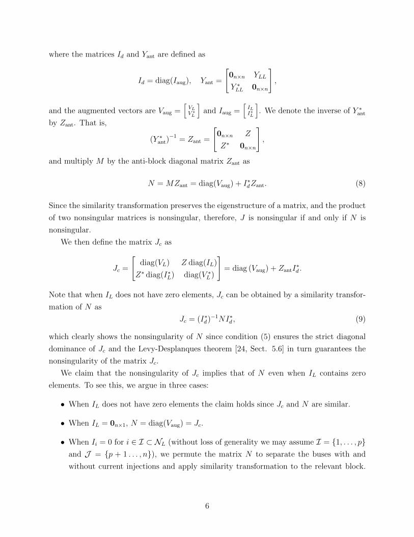
where the matrices Id and Yant are defined as
Id = diag(Iaug), Yant =
[0n×n YLL
Y ∗LL 0n×n
],
and the augmented vectors are Vaug =[VLV ∗L
]and Iaug =
[ILI∗L
]. We denote the inverse of Y ∗ant
by Zant. That is,
(Y ∗ant)−1 = Zant =
[0n×n Z
Z∗ 0n×n
],
and multiply M by the anti-block diagonal matrix Zant as
N = MZant = diag(Vaug) + I∗dZant. (8)
Since the similarity transformation preserves the eigenstructure of a matrix, and the product
of two nonsingular matrices is nonsingular, therefore, J is nonsingular if and only if N is
nonsingular.
We then define the matrix Jc as
Jc =
[diag(VL) Z diag(IL)
Z∗ diag(I∗L) diag(V ∗L )
]= diag (Vaug) + ZantI
∗d .
Note that when IL does not have zero elements, Jc can be obtained by a similarity transfor-
mation of N as
Jc = (I∗d)−1NI∗d , (9)
which clearly shows the nonsingularity of N since condition (5) ensures the strict diagonal
dominance of Jc and the Levy-Desplanques theorem [24, Sect. 5.6] in turn guarantees the
nonsingularity of the matrix Jc.
We claim that the nonsingularity of Jc implies that of N even when IL contains zero
elements. To see this, we argue in three cases:
• When IL does not have zero elements the claim holds since Jc and N are similar.
• When IL = 0n×1, N = diag(Vaug) = Jc.
• When Ii = 0 for i ∈ I ⊂ NL (without loss of generality we may assume I = {1, . . . , p}and J = {p + 1 . . . , n}), we permute the matrix N to separate the buses with and
without current injections and apply similarity transformation to the relevant block.
6

Specifically, define the permutation matrix
P =
Ip 0 0 0
0 0 In−p 0
0 Ip 0 0
0 0 0 In−p
,
where the subscripts of zero matrices are omitted. Then it can be verified that the
permuted matrix P TNP is
P TNP =
[diag(VI) 0
R Nred
],
where
VI =
[VI
V ∗I
], Nred =
[diag(VJ ) diag(I∗J )ZJJ
diag(IJ )Z∗JJ diag(V ∗J )
].
We can now perform similarity transformation on Nred analogous to (9) and condition
(5) applied on the resulting matrix ensures its diagonal dominance, which implies the
nonsingularity of Nred. In addtion, since diag(VI) is nonsingular, it is easy to see
P TNP , thus N , is also nonsingular. We have then proved the claim.
In summary, we have shown that condition (5) implies the nonsingularity of Jc, which in
turn implies the nonsingularity of J . This completes the proof.
4 A New Model for VSC-OPF
The standard AC-OPF formulation embeds system security constraints as line real power
and current limits in (4g) and (4h). However, the parameters in these security-related
constraints, such as P ij and I ij, are calculated off-line using possible dispatch scenarios that
do not necessarily represent the actual system conditions [25]. This motivates the formulation
of VSC-OPF models such as the one using MSV of the power flow Jacobian [15]. However
as noted in the literature, it is numerically difficult to handle the singular value constraints
[16, 17]. In this section, we propose a new model for VSC-OPF using the voltage condition
derived in (5) and show that it has nice convex properties amenable for efficient computation.
7

4.1 New formulation
We propose the following new VSC-OPF model,
min∑i∈NG
fi(PGi) (10a)
s.t. (4b) – (4f)
|Vi| −n∑j=1
|Zij||Sj||Vj|
≥ ti, i ∈ NL. (10b)
The key constraint is (10b), which reformulates the left-hand side of (5) by writing line
currents as the ratio of apparent powers that satisfy the power flow equations (3) and volt-
ages, and ti is a preset positive parameter to control the level of voltage stability. To ensure
that (10) is a proper formulation with good computational property, we first show that the
set of voltages satisfying condition (10b) is voltage stable, and then we show that (10b) is
second-order cone (SOC) representable, thus convex, when SL is constant. The condition of
constant SL is always met in OPF problems.
4.1.1 Connectedness
A necessary condition for voltage instability is the singularity of power flow Jacobian [26,
Sect. 7.1.2]. Assume that the zero injection solution of power flow equations (3) is voltage
stable with a nonsingular Jacobian (we see from (8) that this implies all load voltage magni-
tudes are nonzero since otherwise N is singular). We know from (6) that every entry of J is a
continuous function of voltages, so the eigenvalues of J are also continuous in voltages. Since
a continuous function maps a connected set to another connected set, if a given connected
set of power flow solutions contains the zero injection solution (which is voltage stable) and
the corresponding power flow Jacobian of every point in the set is nonsingular, then the set
characterizes a subset of voltage stable solutions. Define the set S0 := {VL| (5) holds} and
S0 ⊇ St := {VL| (10b) holds}. We know from Theorem 1 that the power flow Jacobian is
nonsingular for VL ∈ S0, we also know the zero injection solution is in S0. Therefore, in order
to show the set St is voltage stable, we show the more general case that S0 is voltage stable,
which amounts to showing the connectedness of S0. We give the proof of this property below.
Theorem 2. The set S0 is connected.
Proof. Given any v1 ∈ S0, and let the zero injection solution be v0 ∈ S0. Define VL
parametrized by t ∈ [0, 1] as VL(t) = v0 + (v1 − v0) t. With the definition we find that
8

current injections are linear functions of t, since
IL(t) = YLL (VL(t)− E) (11a)
= YLL (x0 + (x1 − x0) t− x0) (11b)
= YLL (x1 − x0) t. (11c)
We claim that the derivative of |Vi| has smaller magnitude than the derivative of∑n
j=1 |ZijIj|for all i ∈ NL. Since current injections are linear in t, let ZijIj be denoted by aijt+ ibijt and
Ei by Ei + iFi. Then |Vi| can be represented by
|Vi| =∣∣Ei − zTi Ii∣∣ =
√(Ei −
∑nj=1 aijt
)2+(Fi −
∑nj=1 bijt
)2, (12)
and the derivative of |Vi| with respect to t is (where we shorthand∑n
j=1 aij by a for brevity)
d|Vi|dt
= − a(ei − at) + b(fi − bt)√(ei − at)2 + (fi − bt)2
. (13)
Then, by Cauchy-Schwarz inequality we have |d|Vi|/dt| ≤√a2 + b2. On the other hand,
the derivative of∑n
j=1 |ZijIj| is d/dt∑n
j=1 |ZijIj| =∑n
j=1
√a2ij + b2ij ≥
√a2 + b2, where
the inequality is due to successive application of trigonometric inequality. Comparing the
two derivatives confirms the claim that the derivative of |Vi| has smaller magnitude than the
derivative of∑n
j=1 |ZijIj| for all i ∈ NL. Since the function |Vi|−∑n
j=1 |ZijIj| is monotonically
decreasing, we see the line segment connecting v0 and v1 lies in S0.
4.1.2 SOC representation of voltage stability constraint
The voltage stability constraint (10b) is not directly a convex constraint in the voltage
variable Vi, however, we show that it can be reformulated as a convex constraint, more
specifically, an SOC constraint in squared voltage magnitude |Vi|2 providing SL is fixed.
This SOC reformulation will be utilized in the following section for SOCP relaxation of
VSC-OPF.
Proposition 1. Constraint (10b) is SOC representable in the squared voltage magnitude
|Vi|2’s, i.e. (10b) can be reformulated using SOC constraints in |Vi|2’s.
Proof. First of all, introduce variable cii := |Vi|2, and xi, yi for each bus i ∈ NL such that
xi ≤√cii, (14)
xiyi ≥ 1, (15)
9

xi ≥ 0.
Then we see both (14) and (15) can be rewritten as the following SOC constraints√x2i +
(cii − 1)2
4≤ cii + 1
2,√
1 +(xi − yi)2
4≤ xi + yi
2.
Therefore, by defining Aij = |ZijSj|, ((10b)) can be equivalently represented as
xi −n∑j=1
Aijyj ≥ ti, (16a)
∥∥[xi, (cii − 1)/2]T∥∥2≤ (cii + 1)/2, (16b)∥∥[1, (xi − yi)/2]T
∥∥2≤ (xi + yi)/2, (16c)
xi ≥ 0, (16d)
for every bus i ∈ NL, which are SOCP constraints.
4.2 SOCP relaxation of VSC-OPF
By Proposition 1, the voltage stability condition (5) is reformulated as SOCP constraints
(16). However, the power flow equations (4b)-(4c) are still nonconvex. In the following, we
propose an SOCP relaxation of the proposed VSC-OPF model (10) by combining the SOC
reformulation of the voltage stability constraint (16) with the recent development of SOCP
relaxation of standard AC-OPF [27]. In particular, for each line (i, j) ∈ E , define
cij = eiej + fifj (17a)
sij = eifj − ejfi. (17b)
An implied constraint of (17a)-(17b) is the following:
c2ij + s2ij = ciicjj. (18)
Now we can introduce the following SOCP relaxation of the VSC-OPF model (10) in the
new variables cii, cij, and sij as follows
min∑i∈NG
fi(PGi)
10
s.t. PGi− PDi
= Giicii +∑j∈N(i)
Pij, i ∈ N (19a)
QGi−QDi
= −Biicii +∑j∈N(i)
Qij, i ∈ N (19b)
V 2i ≤ cii ≤ V
2
i , i ∈ N (19c)
cij = cji, sij = −sji, (i, j) ∈ E (19d)
c2ij + s2ij ≤ ciicjj (i, j) ∈ E (19e)
(4d), (4e), (16),
where the power flow equations (4b)-(4c) are rewritten in the c, s variables as (19a) and
(19b). N(i) denotes the set of buses adjacent to bus i. The line real and reactive powers are
Pij = Gijcij − Bijsij and Qij = −Gijsij − Bijcij. The nonconvex constraint (18) is relaxed
as (19e), which can be easily written as an SOCP constraint as ‖[cij, sij, (cii − cjj)/2]T‖2 ≤(cii + cjj)/2. (19c) is a linear constraint in the square voltage magnitude cii. Notice that the
SOCP formulation of the voltage stability constraint (16) is not a relaxation, but an exact
formulation of the original voltage stability condition (10b), and it fits nicely into the overall
SOCP relaxation of the VSC-OPF model (19).
4.3 Sparse approximation of SOCP relaxation
It is observed through experiments that the computation times of the VSC-OPF formula-
tion (19) are significantly longer than normal OPF especially for larger instances, which
is primarily due to the density of stability condition (16a). To speed up computation, we
approximate the coeffcient matrix A of the stability constraints by a sparse matrix A. To
illustrate our approach of sparse approximation, we rewrite the linear constraint (16a) in
matrix-vector form as
x− Ay ≥ t. (20)
Then the approach to construct the sparse approximate matrix A can be summarized as
follows.
Simply put, for each row of matrix A, Algorithm 1 constructs the corresponding row
of the approximate matrix A by ignoring all elements except the largest ones whose sum
amounts to more than γ of the total row sum. We notice that the element Zij of the
impedance matrix can be understood as the coupling intensity measure between buses i and
j. Thanks to the sparsity of practical power systems, each bus is only strongly coupled with
its neighboring buses and weakly coupled with most other buses. Therefore, the matrix A is
generally sparse. We notice a similar approximation has been applied to the L-index in the
11

Algorithm 1 Sparse approximation of A
γ ← 0.98 . initialize tunable sparsity parameterA← 0n×n . initialize Afor 1 ≤ i ≤ n do
RS ←∑
j Aij . compute ith row sum of matrix A
while∑
j Aij < γRS dojmax ← arg max aiAi,jmax ← Ai,jmax
Ai,jmax ← 0end while
end for
context of PMU allocation [28]. The connection between L-index and the proposed stability
condition has been discussed in [22].
Then (20) can be approximated by
x− Ay ≥ t+ ∆a/V , (21)
where ∆a ∈ Rn is the row sum difference between A and A that is defined as ∆ai =∑
(ai−ai)and V = max{V i | i ∈ NL}. We have thus obtained the sparse VSC-OPF formulation
which is identical to (19) except the stability constraint (16a) is replaced by (21). The new
formulation is presented as
min∑i∈NG
fi(PGi)
s.t. PGi− PDi
= Giicii +∑j∈N(i)
Pij, i ∈ N (22a)
QGi−QDi
= −Biicii +∑j∈N(i)
Qij, i ∈ N (22b)
V 2i ≤ cii ≤ V
2
i , i ∈ N (22c)
cij = cji, sij = −sji, (i, j) ∈ E (22d)
c2ij + s2ij ≤ ciicjj (i, j) ∈ E (22e)
(4d), (4e), (16b)–(16d), (21)
We notice that feasibility of problem (22) is implied by the feasibility of the original
problem (19). To see this we only need to focus on (21) and (16a), from which we have
x− Ay ≤ x− Ay − (∆a)ymin
12

≤ x− Ay −∆a/V ,
where the last inequality comes from (14), (15), (19c).
5 Computational Experiments
In this section, we present extensive computational results on the proposed VSC-OPF model
(10), its SOCP relaxation (19), and the sparse approximation (22) tested on standard IEEE
instances available from Matpower [29] and instances from the NESTA 0.6.0 archive [30].
The code is written in Matlab. For all experiments, we used a 64-bit computer with
Intel Core i7 CPU 2.60GHz processor and 4 GB RAM. We study the effectiveness of the
proposed VSC-OPF on achieving voltage stability, the tightness of the SOCP relaxation for
the VSC-OPF, as well as the speed-up and accuracy of the sparse approximation.
Two different solvers are used for VSC-OPF:
• Nonlinear interior point solver IPOPT [31] is used to find local optimal solutions to
VSC-OPF.
• Conic interior point solver MOSEK 7.1 [32] is used to solve the SOCP relaxation of
VSC-OPF.
5.1 Method
For each test case, we choose the margin ti in constraint (16a) by running a base case power
flow based on the given system loading and dispatch information. We obtain the stability
margin for each load bus as
ti = |Vi| −∑j∈NL
Aij|Vj|
, i ∈ NL.
Then, the thresholds ti are obtained as the minimum of ti,
ti = min{ti, i ∈ NL}, i ∈ NL.
That is, we use the stability margin given by the base case power flow result as the stability
threshold for all load buses.
13
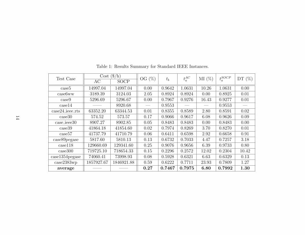
Table 1: Results Summary for Standard IEEE Instances.
Test CaseCost ($/h)
OG (%) tb tACa MI (%) tSOCPa DT (%)AC SOCP
case5 14997.04 14997.04 0.00 0.9642 1.0631 10.26 1.0631 0.00case6ww 3189.39 3124.03 2.05 0.8924 0.8924 0.00 0.8925 0.01
case9 5296.69 5296.67 0.00 0.7967 0.9276 16.43 0.9277 0.01case14 —— 8920.68 — 0.9553 — — 0.9553 —
case24 ieee rts 63352.20 63344.53 0.01 0.8355 0.8589 2.80 0.8591 0.02case30 574.52 573.57 0.17 0.9066 0.9617 6.08 0.9626 0.09
case ieee30 8907.27 8902.85 0.05 0.8483 0.8483 0.00 0.8483 0.00case39 41864.18 41854.60 0.02 0.7974 0.8269 3.70 0.8270 0.01case57 41737.79 41710.79 0.06 0.6411 0.6598 2.92 0.6658 0.91
case89pegase 5817.60 5810.13 0.13 0.6732 0.7033 4.47 0.7257 3.18case118 129660.69 129341.60 0.25 0.9076 0.9656 6.39 0.9733 0.80case300 719725.10 718654.33 0.15 0.2296 0.2572 12.02 0.2304 10.42
case1354pegase 74060.41 73998.93 0.08 0.5928 0.6321 6.63 0.6329 0.13case2383wp 1857927.67 1846921.88 0.59 0.6222 0.7711 23.93 0.7809 1.27average —— —— 0.27 0.7467 0.7975 6.80 0.7992 1.30
14
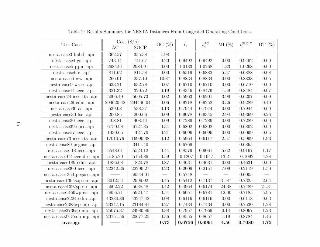
Table 2: Results Summary for NESTA Instances From Congested Operating Conditions.
Test CaseCost ($/h)
OG (%) tb tACa MI (%) tSOCPa DT (%)AC SOCP
nesta case3 lmbd api 362.57 355.38 1.98 — — — — —nesta case4 gs api 743.14 741.67 0.20 0.9492 0.9492 0.00 0.9492 0.00
nesta case5 pjm api 2984.91 2984.91 0.00 1.0133 1.0268 1.33 1.0268 0.00nesta case6 c api 811.62 811.58 0.00 0.6519 0.6882 5.57 0.6888 0.08
nesta case6 ww api 266.01 237.10 10.87 0.8834 0.8834 0.00 0.8838 0.05nesta case9 wscc api 633.21 632.78 0.07 0.6710 0.6710 0.00 0.6710 0.00nesta case14 ieee api 321.32 320.72 0.19 0.8346 0.8479 1.59 0.8484 0.07
nesta case24 ieee rts api 5006.49 5005.73 0.02 0.5963 0.6201 3.99 0.6207 0.09nesta case29 edin api 294620.42 294446.04 0.06 0.9218 0.9252 0.36 0.9289 0.40nesta case30 as api 539.08 538.37 0.13 0.7944 0.7944 0.00 0.7944 0.00nesta case30 fsr api 200.85 200.66 0.09 0.9078 0.9345 2.94 0.9369 0.26nesta case30 ieee api 408.81 408.44 0.09 0.7289 0.7289 0.00 0.7289 0.00nesta case39 epri api 6750.98 6727.85 0.34 0.6802 0.6802 0.00 0.6802 0.00nesta case57 ieee api 1430.65 1427.70 0.21 0.6096 0.6096 0.00 0.6099 0.05
nesta case73 ieee rts api 17010.76 16990.38 0.12 0.5964 0.6117 2.57 0.5999 1.93nesta case89 pegase api —— 3411.40 — 0.6769 — — 0.6865 —nesta case118 ieee api 5548.61 5524.12 0.44 0.8579 0.9061 5.62 0.9167 1.17
nesta case162 ieee dtc api 5185.20 5154.86 0.59 -0.1207 -0.1047 13.21 -0.1092 4.28nesta case189 edin api 1836.68 1820.78 0.87 0.4631 0.4631 0.00 0.4631 0.00nesta case300 ieee api 22342.36 22290.27 0.23 0.2009 0.2151 7.09 0.2119 1.50
nesta case1354 pegase api —— 59544.01 — 0.5748 — — 0.6005 —nesta case1394sop eir api 3012.54 2999.02 0.45 0.5412 0.7137 31.87 0.7325 2.64nesta case1397sp eir api 5662.22 5638.48 0.42 0.4964 0.6174 24.38 0.7489 21.31nesta case1460wp eir api 5956.71 5924.47 0.54 0.6051 0.6781 12.06 0.7185 5.95nesta case2224 edin api 43280.89 43247.42 0.08 0.6116 0.6116 0.00 0.6118 0.03
nesta case2383wp mp api 23247.15 23184.81 0.27 0.7434 0.7434 0.00 0.7530 1.28nesta case2736sp mp api 25075.37 24980.89 0.38 0.7957 0.7969 0.14 0.8067 1.23nesta case2737sop mp api 20751.56 20677.25 0.36 0.8555 0.8657 1.19 0.8784 1.46
average —— —— 0.73 0.6756 0.6991 4.56 0.7080 1.75
15

Table 3: Results Summary of Sparse Approximation for NESTA Instances From Congested Operating Conditions.
Test CaseTime (sec)
DCT (%) Cost ($/h) DC (%) tsa DT (%)Normal Sparse
nesta case3 lmbd api 0.70 0.68 1.98 355.38 0.00 — —nesta case4 gs api 0.73 0.74 -1.54 741.67 0.00 0.9492 0.00
nesta case5 pjm api 0.70 0.70 0.79 2984.91 0.00 1.0268 0.00nesta case6 c api 0.72 0.72 0.74 811.58 0.00 0.6888 0.00
nesta case6 ww api 0.76 0.76 0.03 237.10 0.00 0.8838 0.00nesta case9 wscc api 0.91 0.80 12.59 626.86 0.94 0.6694 0.25nesta case14 ieee api 0.75 0.71 4.97 320.72 0.00 0.8484 0.00
nesta case24 ieee rts api 0.78 0.78 0.53 5005.73 0.00 0.6207 0.00nesta case29 edin api 0.85 0.85 0.40 294446.03 0.00 0.9289 0.00nesta case30 as api 0.70 0.72 -2.69 538.37 0.00 0.7940 0.05nesta case30 fsr api 0.70 0.71 -1.21 200.66 0.00 0.9369 0.00nesta case30 ieee api 0.71 0.69 2.56 408.44 0.00 0.7287 0.03nesta case39 epri api 0.86 0.84 1.62 6727.02 0.01 0.6800 0.02nesta case57 ieee api 0.75 0.74 0.50 1427.70 0.00 0.6099 0.00
nesta case73 ieee rts api 0.76 0.81 -5.87 16990.51 0.00 0.5999 0.00nesta case89 pegase api 0.91 0.94 -3.71 3411.40 0.00 0.6865 0.00nesta case118 ieee api 0.83 0.83 -0.23 5524.12 0.00 0.9167 0.00
nesta case162 ieee dtc api 0.97 0.94 3.31 5154.86 0.00 -0.1092 0.00nesta case189 edin api 1.04 1.03 0.96 1817.51 0.18 0.4626 0.10nesta case300 ieee api 1.80 1.20 33.39 22292.03 0.01 0.2023 4.51
nesta case1354 pegase api 25.04 4.24 83.05 59543.72 0.00 0.6005 0.00nesta case1394sop eir api 39.44 9.75 75.27 2999.03 0.00 0.7325 0.00nesta case1397sp eir api 40.42 10.34 74.42 5638.34 0.00 0.7489 0.00nesta case1460wp eir api 39.95 10.54 73.61 5924.42 0.00 0.7184 0.00nesta case2224 edin api 274.68 22.23 91.91 43247.11 0.00 0.6116 0.03
nesta case2383wp mp api 90.54 6.92 92.35 23184.84 0.00 0.7529 0.00nesta case2736sp mp api 496.59 14.92 97.00 24980.71 0.00 0.8066 0.00nesta case2737sop mp api 1190.98 35.29 97.04 20676.94 0.00 0.8784 0.00
average 79.09 4.66 26.20 — 0.04 0.7027 0.19
16

5.2 Results and discussions
The results of our computational experiments on VSC-OPF and its SOCP relaxation are
presented in Tables 1 and 2 for standard IEEE and NESTA instances, respectively. The
“Cost” columns in both tables show the objective values of the VSC-OPF model (10) and
its SOCP relaxation (19). In addition, six sets of information are provided in Tables 1 and
2:
• OG(%) is the percentage optimality gap between the lower bound LB obtained from
the SOCP relaxation of VSC-OPF (19) and an upper bound UB obtained by IPOPT.
It is calculated as 100%× (1− LB/UB).
• tb is the minimum value of |Vi|−∑n
j=1 aij/|Vj| for all load bus i calculated in the based
case before solving VSC-OPF.
• tACa is the minimum value of |Vi| −∑n
j=1 aij/|Vj| for all load bus i calculated after
solving VSC-OPF (10).
• MI(%) is the percent increase of stability margin measured as 100%× |tACa /tb − 1|.
• tSOCPa is the minimum value of |Vi| −∑n
j=1 aij/|Vj| for all load bus i calculated after
solving SOCP relaxation of VSC-OPF.
• DT(%) is the percent difference between tACa and tSOCPa calculated as 100%×|tSOCPa /tACa −1|.
5.2.1 Stability margin improvement
As shown by Tables 1 and 2, on average, the proposed VSC-OPF improves the voltage
stability margin by 6.80% for the IEEE instances and 3.48% for the NESTA instances over the
standard OPF shown in tb column. We also see that several test instances have significantly
larger improvement. For example, the 300-bus system and the 2383-bus system in Table
1 have 12.02% and 23.93% improvement; the 162-bus, 1394-bus, 1397-bus, and 1406-bus
systems in the NESTA archive all have more than 10% to 30% improved stability margin
than the standard OPF model.
As a more specific example, we observe that for NESTA 162-bus system, the sufficient
voltage stability condition (5) is violated at the base operating condition by at least one
bus. The condition being violated signifies a severe system stress level and a low margin. In
fact, the NESTA 162-bus system is indeed quite close to its solvability boundary in the base
case, even though all voltages are within 6% of the nominal value. The result confirms our
17

discussion in Section 1 that conventional security constraints such as voltage magnitude limits
are not always sufficient in reflecting true system margin and a more systematic measure
should be enforced.
5.2.2 Tightness of SOCP relaxation
Tables 1-2 both show that the optimality gap between the SOCP relaxation (19) and a
local solution of the non-convex VSC-OPF (10) is very small: 0.27% and 0.73% for the
IEEE and NESTA instances, respectively. It is curious to compare to the optimality gap
of the SOCP relaxation of the standard OPF model. In fact, the gaps are much smaller
compared to that for the conventional OPF problem for the NESTA instances, which presents
more computational challenge than the standard IEEE instances. In particular, the average
optimality gap of SOCP relaxation for standard OPF is 6.19%, compare to 0.73% for the
VSC-OPF problem shown in Table 2. Specifically, only two instances have optimality gaps
larger than 1% in Table 2, while the number for the SOCP relaxation of standard OPF
problem is 18 instances. For IEEE instances, the average optimality gaps are similar: 0.25%
for standard OPF versus 0.27% for VSC-OPF. This can be attributed to the fact that the
flow limits for IEEE instances are high and most of them are not binding.
5.2.3 Effect of sparse approximation
The results of our computational experiments on the sparse approximation of VSC-OPF for
NESTA instances are presented in Table 3. The sparsity parameter in Algorithm 1 is chosen
to be 0.98. The “Time” columns in the table show the computation time of the VSC-OPF
model (19) and the sparse approximation (22). In addition, the table reports five sets of
data as described below:
• DCT(%) is the percentage time difference between the computation time ctn of (19)
and cts of (22). It is calculated as 100%× (1− cts/ctn).
• Cost($/h) is the objective value of the sparse approximation (22).
• DC(%) is the percentage difference between the objective value cSOCP of the model
(19) and cs of (22) calculated as 100%× |cs/cSOCP − 1|.
• tsa is the minimum value of |Vi|−∑n
j=1 aij/|Vj| for all load bus i calculated after solving
(22).
• DT(%) is the percentage difference between tSOCPa and tsa calculated as 100%×|tsa/tSOCPa −1|.
18

For systems with less than five buses, the sparse approximation (22) and the original
SOCP relaxation model (19) are exactly the same. For system sizes ranging between 6-bus
and 300-bus, the computation times of model (19) are sufficiently short (less than 2 seconds),
which render the sparse approximation unnecessary. However, for systems with more than
1000 buses, the sparse approximation brings about significant speed-up. In fact, the speed-
ups are above 90% for all instances with more than 2000 buses and the optimal solutions
are obtained in less than 36 seconds for all instances. As can be seen from the columns
of DC(%) and DT(%), the solution accuracies are extremely high. For larger systems with
more than 1000 buses, the differences of cost and stability margin between (19) and (22) are
all less than 0.01% except the margin difference for 2224-bus system, which is 0.03%.
6 Conclusions
We have presented a sufficient condition for power flow Jacobian nonsingularity and have
given a new proof for the condition. We have also shown that the condition characterizes
a set of voltage stable solutions. A new VSC-OPF model has been proposed based on the
sufficient condition. By using the fact that the load powers are constant in an OPF problem,
we reformulate the voltage stability condition to a set of second-order conic constraints in a
transformed variable space. Furthermore, in the new variable space, we have formulated an
SOCP relaxation of the VSC-OPF problem as well as its sparse approximation. Simulation
results show that the proposed VSC-OPF and its SOCP relaxation can effectively restrain
the stability stress of the system; the optimality gap of the SOCP relaxation is much smaller
compared to SOCP relaxation of the standard OPF problem on difficult instances; and the
sparse approximation yields significant speed-up on larger instances with hardly any accuracy
compromise.
References
[1] P. W. Sauer and M. A. Pai, “Power system steady-state stability and the load-flow
Jacobian,” IEEE Trans. Power Syst., vol. 5, no. 4, pp. 1374–1381, Nov. 1990.
[2] I. A. Hiskens and R. J. Davy, “Exploring the power flow solution space boundary,”
IEEE Trans. Power Syst., vol. 16, no. 3, pp. 389–395, Aug. 2001.
[3] V. Ajjarapu and C. Christy, “The continuation power flow: a tool for steady state
voltage stability analysis,” IEEE Trans. Power Syst., vol. 7, no. 1, pp. 416–423, Feb.
1992.
19

[4] T. Van Cutsem, “A method to compute reactive power margins with respect to voltage
collapse,” IEEE Trans. Power Syst., vol. 6, no. 1, pp. 145–155, Feb. 1991.
[5] F. F. Wu and S. Kumagai, “Steady-state security regions of power systems,” IEEE
Trans. Circuits Syst., vol. 29, no. 11, pp. 703–711, Nov. 1982.
[6] M. Ilic, “Network theoretic conditions for existence and uniqueness of steady state
solutions to electric power circuits,” in Proc. ICSAS, San Diego, CA, USA, 1992, pp.
2821–2828.
[7] S. Bolognani and S. Zampieri, “On the existence and linear approximation of the power
flow solution in power distribution networks,” IEEE Trans. Power Syst., vol. 31, no.
1, pp. 163–172, Jan. 2016.
[8] S. Yu, H. D. Nguyen, and K. S. Turitsyn, “Simple certificate of solvability of power
flow equations for distribution systems,” in Proc. IEEE Power Eng. Soc. Gen. Meeting,
Jul. 26–30, 2015.
[9] J. W. Simpson-Porco, F. Dorfler, and F. Bullo, “Voltage collapse in complex power
grids,” Nature Commun., vol. 7, 2016, Art. no. 10790.
[10] C. Wang, A. Bernstein, J.-Y. Le Boudec, and M. Paolone, “Explicit conditions on
existence and uniqueness of load-flow solutions in distribution networks,” IEEE Trans.
Smart Grid, to be published.
[11] J. W. Simpson-Porco, “A theory of solvability for lossless power flow equations — part
i: fixed-point power flow,” arXiv preprint arXiv: 1701.02045, 2017.
[12] J. W. Simpson-Porco, “A theory of solvability for lossless power flow equations — part
ii: existence and uniqueness,” arXiv preprint arXiv: 1701.02047, 2017.
[13] K. Vu, M. M. Begovic, D. Novosel, and M. M. Saha, “Use of local measurements
to estimate voltage-stability margin,” IEEE Trans. Power. Syst., vol. 14, no. 3, pp.
1029–1034, Aug. 1999.
[14] Y. Wang, I. R. Pordanjani, W. Li, W. Xu, T. Chen, E. Vaahedi, and J. Gurney,
“Voltage stability monitoring based on the concept of coupled single-port circuit,”
IEEE Trans. Power Syst., vol. 26, no. 4, pp. 2154–2163, Nov. 2011.
[15] C. Canizares, W. Rosehart, A. Berizzi, and C. Bovo, “Comparison of voltage security
constrained optimal power flow techniques,” in Proc. IEEE PES Summer Meeting,
Vancouver, BC., Canada, July 2001.
20

[16] S. K. M. Kodsi and C. A. Canizares, “Application of a stability-constrained optimal
power flow to tuning of oscillation controls in competitive electricity markets,” IEEE
Trans. Power Syst., vol. 22, no. 4, pp. 1944–1954, Nov. 2007.
[17] R. J. Avalos, C. A. Canizares, and M. F. Anjos, “A practical voltage-stability-
constrained optimal power flow,” in Proc. IEEE PES General Meeting, Jul. 2008.
[18] V. S. S. Kumar, K.K. Reddy, and D. Thukaram, “Coordination of reactive power in
grid-connected wind farms for voltage stability enhancement,” IEEE Trans. Power
Syst., vol. 29, no. 5, pp. 2381–2390, Sep. 2014.
[19] A. S. Pedersen, M. Blanke, and H. Johannsson, “Convex relaxation of power dispatch
for voltage stability improvement,” in Proc. IEEE Multi-Conference on Systems and
Control, Sydney, Australia, Sep. 2015 pp. 1528–1533.
[20] M. Chavez-Lugo, C. R. Fuerte-Esquivel, C. A. Canizares, and V. J. Gutierrez-
Martinez, “Practical security boundary-constrained DC optimal power flow for elec-
tricity markets,” IEEE Trans. Power Syst., vol. 31, no. 5, pp. 3358–3368, Sep. 2016.
[21] M. Todescato, J. W. Simpson-Porco, F. Dorfler, R. Carli, and F. Bullo, “Optimal
voltage support and stress minimization in power networks,” in Proc. IEEE Conf.
Decision Control, Osaka, Japan, Dec. 2015, pp. 6921–6926.
[22] Z. Wang, B. Cui, and J. Wang, “A necessary condition for power flow insolvability
in power distribution systems with distributed generators,” IEEE Trans. Power Syst.,
vol. 32, no. 2, pp. 1440–1450, Mar. 2017.
[23] P. Kessel and H. Glavitsch, “Estimating the voltage stability of a power system,” IEEE
Trans. Power Del., vol. 1, no. 3, pp. 346–354, Jul. 1986.
[24] R. A. Horn and C. R. Johnson, Matrix Analysis, Cambridge University Press, 2013.
[25] F. Milano, C. A. Canizares, and M. Invernizzi, “Multi-objective optimization for pric-
ing system security in electricity markets,” IEEE Trans. Power Syst., vol. 18, no. 2,
pp. 596–604, May 2003.
[26] T. Van Cutsem and C. Vournas, Voltage Stability of Electric Power Systems. New
York, NY, USA: Springer, 2008.
[27] B. Kocuk, S. Dey, and X. A. Sun, “Strong SOCP relaxation for the optimal power
flow problem,” Operations Research, vol. 64(6), 1177–1196, 2016.
21

[28] I. R. Pordanjani, Y. Wang, and W. Xu, “Identification of critical components for
voltage stability assessment using channel components transform,” IEEE Trans. Smart
Grid, vol. 4, no. 2, pp. 1122–1132, Jun. 2013.
[29] R. D. Zimmerman, C. E. Murillo-Sanchez, and R. J. Thomas, “MATPOWER: steady-
state operations, planning and analysis tools for power systems research and educa-
tion,” IEEE Trans. Power Syst., vol. 26, no. 1, pp. 12–19, Feb. 2011.
[30] C. Coffrin, D. Cordon, and P. Scott, “NESTA, the NICTA energy system test case
archive,” arXiv preprint arXiv: 1411.0359, 2014.
[31] A. Wachter and L. T. Biegler, “On the implementation of an interior-point filter line-
search algorithm for large-scale nonlinear programming,” Math. Prog., vol. 106, no. 1,
pp. 25–57, 2006.
[32] MOSEK, MOSEK Modeling Manual, MOSEK ApS, 2013.
22


