
A New Deep-Beam Element for Mixed-Type Modeling of Concrete Structures
Jian Liu, Ph.D. Candidate, Liège Dr. Serhan Guner, Assistant Professor, Toledo Dr. Boyan Mihaylov, Assistant Professor, Liège
Department of ArGEnco, University of Liège, Belgium Department of Civil Engineering, The University of Toledo, Ohio, USA
2016, 2021 © (This research was conducted in 2016; this report was released in 2021.)

ii
Contents 1 Introduction ............................................................................................................................. 1
1.1 What are deep beams? ...................................................................................................... 1
1.2 Problems with modelling large frame structures with deep beams included ................... 1
1.3 Solution proposed ............................................................................................................. 2
2 Formulation of a Deep-Beam Element based on 3PKT .......................................................... 2
2.1 Brief introduction on 3PKT.............................................................................................. 2
2.2 Formulation of 1D deep element ...................................................................................... 3
2.3 Solution scheme of 1D deep element ............................................................................... 5
2.4 Subroutine DPBM for 1D deep element .......................................................................... 6
2.5 Adaption of the deep element into VecTor5 .................................................................... 7
3 A New Member Type in VecTor5 ........................................................................................... 7
3.1 Description of Type-8 member ........................................................................................ 7
3.2 User guide: implementation of Type-8 member .............................................................. 7
3.3 Shear protection................................................................................................................ 8
3.4 Output files ....................................................................................................................... 9
4 Verification studies .................................................................................................................. 9
4.1 Simply supported beams ................................................................................................ 10
4.1.1 1st set of tests: Salamy (2005) ................................................................................ 10
4.1.2 2nd set of tests: Tanimura (2005) ........................................................................... 19
4.2 Continuous deep beam ................................................................................................... 22
4.3 Frames ............................................................................................................................ 23
4.3.1 Two-story single-span frame .................................................................................. 23
4.3.2 Two-story two-bay frame ....................................................................................... 27
4.3.3 Force control vs. displacement control ................................................................... 28
5 Future Work ........................................................................................................................... 30
5.1 Axial force ...................................................................................................................... 30
5.2 Unloading/reloading path ............................................................................................... 30
5.3 Automatic detection of deep beam element ................................................................... 30
5.4 Output of crack pattern in Janus ..................................................................................... 30
6 References ............................................................................................................................. 30
Annex 1: Flow chart of subroutine DPBM ................................................................................... 31

1
1 Introduction
1.1 What are deep beams? Deep beams are typically used as transfer girders in high-rise buildings or bridges. An
example is shown in Figure 1, where a deep transfer girder is used to carry the heavy loads
from upper stories to have an open space at the lower story of a large frame structure. The
shear-span-to depth ratio a/d for deep beam is much lower than slender beam, which attributes
to the difference in shear behaviour between these two types of beams. Generally, if a/d is
less than 2.5, the beam is considered to be deep; otherwise, it is slender. Due to this
characteristic, deep beams have disturbed deformation field and do not obey the assumption
of classical beam theory, i.e., ‘plane section remain plane’.
Figure 1: Typical large frame structure with deep beams.
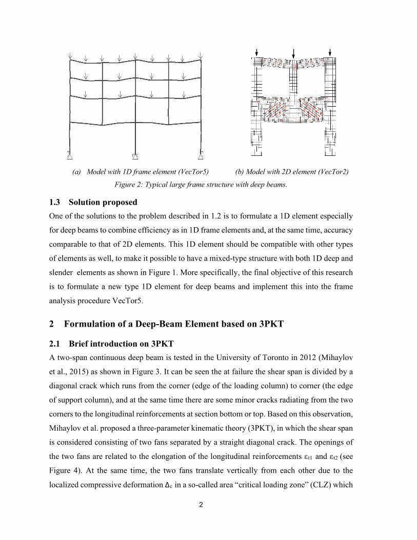
1.2 Problems with modelling large frame structures with deep beams included A frame structure can be modelled either with 1D frame element (e.g., in VecTor5) or with
2D element (e.g., in VecTor2, see Figure 2). The former holds advantage over the latter due
to its efficiency in model formation and calculation as well as its good compatibility with
other elements. However, 1D frame elements are formulated based on the slender beam
theory, and thus cannot provide accurate predictions for deep beams. Despite its inefficiency,
2D element is able to provide relatively accurate predictions. Therefore, it is not an easy task
to model a large frame with deep beams included efficiently and accurately.
transfergirder
deep beam
slenderbeam
da
2
(a) Model with 1D frame element (VecTor5) (b) Model with 2D element (VecTor2)
Figure 2: Typical large frame structure with deep beams.
1.3 Solution proposed One of the solutions to the problem described in 1.2 is to formulate a 1D element especially
for deep beams to combine efficiency as in 1D frame elements and, at the same time, accuracy
comparable to that of 2D elements. This 1D element should be compatible with other types
of elements as well, to make it possible to have a mixed-type structure with both 1D deep and
slender elements as shown in Figure 1. More specifically, the final objective of this research
is to formulate a new type 1D element for deep beams and implement this into the frame
analysis procedure VecTor5.
2 Formulation of a Deep-Beam Element based on 3PKT
2.1 Brief introduction on 3PKT A two-span continuous deep beam is tested in the University of Toronto in 2012 (Mihaylov
et al., 2015) as shown in Figure 3. It can be seen the at failure the shear span is divided by a
diagonal crack which runs from the corner (edge of the loading column) to corner (the edge
of support column), and at the same time there are some minor cracks radiating from the two
corners to the longitudinal reinforcements at section bottom or top. Based on this observation,
Mihaylov et al. proposed a three-parameter kinematic theory (3PKT), in which the shear span
is considered consisting of two fans separated by a straight diagonal crack. The openings of
the two fans are related to the elongation of the longitudinal reinforcements εt1 and εt2 (see
Figure 4). At the same time, the two fans translate vertically from each other due to the
localized compressive deformation Δc in a so-called area “critical loading zone” (CLZ) which

3
is located at one tip of the fan. The complete deformation pattern is the superposition of the
two basic deformation patterns. Refer to Mihaylov (2013) for more details.
Figure 3 Deep beam at failure.
(a) Complete deformation pattern
=
(b) Deformation pattern associated with DOFs εt1,avg and εt2,avg (or θ1 and θ2)
(c) Deformation pattern associated with DOF Δc
Figure 4 Three-parameter kinematic model for shear spans of deep beams under double curvature
2.2 Formulation of 1D deep element 3PKT provides another option for deep beam analysis, and in fact compared with other
theories or models, e.g., strut-and-tie model, plasticity model; it is more suitable for the
formulation of 1D element. As demonstrated in Figure 5, the two fans can be lumped as two
P2
P1
CLZΔc
εt2,avg
εt1,avg1
M2
M1θ2
θ1
a
εt2,avg
εt1,avgθ1
θ2
+Δc
CLZ

4
rotational springs and the rotations are equivalent to the opening angle of the two fans (θ1 and
θ2). The deformation in CLZ Δc can be equivalent to the elongation in a transverse spring
located at the mid-shear-span. The transverse spring, in fact, consists of four parallel springs
which correspond to the four shear mechanisms considered in 3PKT. There are two DOF at
each node, i.e., sectional rotation and vertical displacement. The secant stiffness of the three
springs is k1, k2 and k3, respectively.
(a) Components of the macro-element
(b) Kinematics of the macro-element
Figure 5 Macro element for deep shear spans
Therefore, the stiffness matrix of this 1D deep element can be written as:
( )( ) ( )
( )( ) ( )
12
1 2 3 1 3
1 3 3 1 2 2 3 3 1 22
2 3 2 1 3
2 1 3
21 2
3
3 1 2 2 3
1 2 3 11 3 23 2
-
- - -
-
1
-
-
-
k k k a k k a
k k a k k k k k a k k k
k k k k a
kk k k a k k k k a
k k
k k a k k k a
a kk k k a k k kk
= × + +
+
+ +
+
+ +
(1)
Once the stiffness matrix and boundary condition are known, the shear span can be solved
with the following equation:
11
1
22
2-
MvV
Mv
k
V
ϕ
ϕ
=
(2)
k1 k3 k2
Rigid bar Rigid bar
Section 1 Section 2
a
φ2
v2
φ1
v1 Δc
θ2
θ1
Δc
x
y

5
This 1D deep element is easy being connected with other element either of the same type or
different type. Deep beams can be easily modelled by connecting two or more 1D deep
element as shown in Figure 6 Macro-element model of a continuous deep beam.
Figure 6 Macro-element model of a continuous deep beam
2.3 Solution scheme of 1D deep element Since the secant stiffness of the springs of the macro element changes with the level of
loading, an iterative solution procedure is required to achieve equilibrium between the internal
and external forces at each load stage. The linear system expressed with Eq. (2) can be first
solved with a selected set of secant stiffnesses, for instance those from the previous converged
load stage. This analysis produces deformations θ1, θ2 and Δc in the springs of each macro
element, and these deformations are substituted to calculate new values of the forces in the
springs M1, M2 and V. These forces are in turn used to calculate new secant stiffnesses
k1=M1/θ1, k2=M2/θ2 and k3=V/Δc with which to perform the next linear elastic analysis. The
procedure is repeated until the secant stiffnesses of the springs converge to constant values.
The iterations for a transverse spring in a typical deep beam analysis are demonstrated in
Figure 7. The crosses in the plot show two consecutive converged load stages, while the
inclined lines show the secant stiffness as it changes from iteration to iteration. The
displacement Δc obtained from each linear analysis is marked with a vertical line. The
intersection point between the vertical line and the V-Δc curve is used to define the secant
stiffness for the next iteration. As the iterations progress, the vertical lines become
progressively closer until the solution converges.
P
Section i Section i+1 Section i+2

6
Figure 7 Iteration scheme demonstrated for a transverse spring.
2.4 Subroutine DPBM for 1D deep element Based on the description in the previous section, a subroutine is developed for the deep
element. This subroutine has the displacements at each node as inputs. It should be noticed
that those displacements are in global coordinate system and need to be transformed into the
DOF in local coordinate system for each shear span. At the same time there is one more DOF
included which is the axial displacement of the node, i.e., u. The axial behaviour of the deep
element is assumed to be elastic, i.e., 𝑁𝑁 = 𝐸𝐸𝑐𝑐𝐴𝐴𝑔𝑔𝑢𝑢/𝐿𝐿. Therefore, the outputs are the axial force
AF, shear force BF and bending moment SM. It can be expressed in Figure 8.
Figure 8 The function of subroutine DPBM
u(1) u(2)u(3)
u(4)
u(5)u(6)
xz
yAF
BFBM xz
y
AF
BFBM
Subroutine DPBM
AF
BF
SM
u(1) u(2) u(3)
u(4) u(5) u(6)
Node i:
Node i+1:

7
2.5 Adaption of the deep element into VecTor5 Generally, the bending moments at two ends of the deep element, i.e., M1 and M2, are not
equal (see Equation 2), however, in order to be adapted to the framework of VecTor5, the
bending moment calculated by subroutine DPBM is taken as BM=(M1-M2)/2. At the same
time dowel action is considered explicitly in subroutine DPBM, therefore, the dowel action
in original VecTor5 is skipped in the calculation of shear capacity of deep members. Details
are not meant to be mentioned in this report.
3 A New Member Type in VecTor5
3.1 Description of Type-8 member There are seven existing member types in VecTor5, including: nonlinear frame member
(default member), truss member, tension-only member, compression-only member, etc. A
new member type for nonlinear deep member is added into VecTor5, named as ‘Type 8
member’. Similar to the nonlinear frame member (see Figure 9), the new-type member has
three DOFs at each node; i.e., axial displacement, transverse displacement and rotation in the
local coordinate system.
(a) Default nonlinear frame member
(b) New nonlinear deep member
Figure 9 Member reference types in VecTor5
3.2 User guide: implementation of Type-8 member The user should make the decision if there is any deep member in the model. This member
should be defined as Type 8, as shown in Figure 10. All the input files (*.s5r, *.l5r, *.job and

8
*.aux) are created in the same manner as in the original VecTor5 except the following two
aspects. See Bulletin 8: Deep Beam Modeling with VecTor5 <web link> for more information.
1) If Type-8 member is to be used, only one element should be used for one shear span.
There is no need to discretize the shear span.
2) It is necessary to provide data on the loading plate/support width since this is an
important parameter when determining the shear contribution from critical loading
zone calculated in the subroutine DPBM. The required input is shown in Figure 10.
(a) Ref. Type=8 for deep element
(b) Loading plate/support width input
Figure 10 Input related to the Type-8 members.
3.3 Shear protection Shear protection is a scheme in VecTor 5 for approximately suppressing premature failures
in D-regions (disturbed regions). The new Type-8 member explicitly calculates the shear
capacity of deep members; thus, eliminating the need for this scheme. Therefore, it is
necessary to turn off shear protection for Type-8 members. To expedite this, the new
subroutines automatically turn off shear protection for Type-8 members. The user could see
the list of members for which the shear protection on in the *.s5E expanded data file.

9
3.4 Output files The results for Type-8 members are shown in the output files as shown in Figure 11. The three
kinematic parameters in 3PKT and the corresponding internal forces are listed at the
beginning, which is followed by the four shear components. The straight diagonal crack is
described with its inclined angle, slip along the crack as well as the crack opening at the mid-
length of the crack.
Figure 11 Output related with Type-8 member.
4 Verification studies Note: Below sections discuss preliminary verification studies using a force-controlled loading
protocol. Refer to the following publication for the final results, which uses a displacement-
controlled protocol. Liu, J., Guner, S., and Mihaylov, B. (2019) “Mixed-Type Modeling of
Structures with Slender and Deep Beam Elements” ACI Structural Journal, 116(4), pp. 253-
264. <web link>

10
4.1 Simply supported beams
4.1.1 1st set of tests: Salamy (2005) The first group of specimens from Salamy (2005 are under symmetrical 4-point bending (see Figure 12). The external two spans sustain
high shear while the middle span is under pure flexure. The information of the specimens is listed in Table 1.
Figure 12 Specimens tested by Salamy (2005)
Table 1 Investigated specimens from Salamy (2005)
Beam a/d lb1 b d ρ l
nb fy a
V/P h ag fc ρv fyv Vexp Δexp Vexp
Vpred1 ΔexpΔpred1
Vexp
Vpred2 ΔexpΔpred2
Vexp
Vpred3 ΔexpΔpred3
(mm) (mm) (mm) (%) (MPa) (mm) (mm) (mm) (MPa) (%) (MPa) (kN) (mm)
B-10-2 1.50 100 240 400 2.02 5 376 600 1.0 475 20 23.0 0.00 - 357 6.9 0.22 0.43 0.47 0.25 0.73 0.48
B-13-2 1.50 200 480 800 2.07 10 398 1200 1.0 905 20 24.0 0.00 - 1128 9.0 0.13 0.43 0.40 0.13 0.92 0.66
B15 1.50 300 720 1200 1.99 18 402 1800 1.0 1305 20 27.0 0.00 - 2709 16.0 0.09 0.33 0.37 0.10 0.87 0.58
B17 1.50 250 600 1000 2.04 14 398 1500 1.0 1105 20 28.7 0.40 398 2597 11.8 0.44 0.50 0.80 0.89 0.90 0.87
B18 1.50 350 840 1400 2.05 18 398 2100 1.0 1505 20 23.5 0.40 398 4214 16.3 0.24 0.40 0.78 0.70 1.00 0.86
Avg= 0.22 0.42 0.57 0.41 0.89 0.69
COV= 60.3% 14.1% 36.8% 87.5% 11.3% 25.0%
P P
a a
d h
lb1 lb1

11
Force-control loading is adopted in the modelling to remain under the same condition as in the
experiment.
1) Model 1 in original VecTor5
Modelling the full beam with slender elements:
Figure 13 Model in original VT5
All options are kept as default which is the common situation for users.
2) Model 2 in modified VecTor5
Modeling the deep shear spans with deep elements, the pure flexure span with slender elements:
Figure 14 Model in modified VT5
3) Comparison between Model 1 and Model 2
Crack pattern at the same load stage.
Noted that the crack pattern from model 2 is not reliable since the post-processor Janus is not
modified for displaying deep beam crack patterns yet.
Table 2 Crack pattern comparison between Model 1 and Model 2 at the same load stage
Deep shear span Deep shear span
Pure flexure span
Deep shear span Deep shear span
Pure flexure span
Beam Model Crack pattern
B-10-2
Model 1 (Original VecTor5)
Model 2 (Modified VecTor5)
(LS=31)
(LS=31)

12
B-13-2
Model 1 (Original
VecTor5)
Model 2 (Modified
VecTor5)
B15
Model 1 (Original
VecTor5)
Model 2 (Modified
VecTor5)
B17
Model 1 (Original
VecTor5)
Model 2 (Modified
VecTor5)
B18
Model 1 (Original
VecTor5)
Model 2 (Modified
VecTor5)
(LS=80)
(LS=80)
(LS=120)
(LS=120)
(LS=140)
(LS=140)
(LS=160)
(LS=160)

13
Crack pattern at failure
Table 3 Crack pattern comparison between Model 1 and Model 2 at failure
Beam Model Crack pattern
B-10-2
Model 1 (Original
VecTor5)
Model 2 (Modified
VecTor5)
B-13-2
Model 1 (Original
VecTor5)
Model 2 (Modified
VecTor5)
B15
Model 1 (Original
VecTor5)
Model 2 (Modified
VecTor5)
B17
Model 1 (Original
VecTor5)
Model 2 (Modified
VecTor5)

14
B18
Model 1 (Original
VecTor5)
Model 2 (Modified
VecTor5)
Load-deflection responses
(a) Beam: B102 (b) Beam: B132
(c) Beam: B15 (d) Beam: B17
0
50
100
150
200
250
300
350
400
0 5 10 15 20
Shea
r for
ce V
, kN
Deflection, mm
B10-2
Test
Original VT5
Improved VT5
0
200
400
600
800
1000
1200
0 5 10 15
Shea
r for
ce V
, kN
Deflection, mm
B13-2
Test
Original VT5
Improved VT5
0
500
1000
1500
2000
2500
3000
0 5 10 15 20 25
Shea
r for
ce V
, kN
Deflection, mm
B15
Test
Original VT5
Improved VT5
0
500
1000
1500
2000
2500
3000
0 10 20 30
Shea
r for
ce V
, kN
Deflection, mm
B17
Test
Original VT5
Improved VT5

15
(e) Beam: B18
Figure 15 Load-displacement relationships
Convergence
The following shows the convergence for each beam. It should be noted only those from the
improved VecTor5 are shown.
(a) Beam: B102 (b) Beam: B132
(c) Beam: B15 (d) Beam: B17
0
500
1000
1500
2000
2500
3000
3500
4000
4500
0 5 10 15 20 25
Shea
r for
ce V
, kN
Deflection, mm
B18
Test
Original VT5
Improved VT5
0.99981
1.00021.00041.00061.0008
1.0011.00121.00141.0016
0 10 20 30 40 50 60
Conv
erge
nce
fact
or
Load step
0.9995
1
1.0005
1.001
1.0015
1.002
1.0025
0 10 20 30 40 50 6
Conv
erge
nce
fact
or
Load step
0.9995
1
1.0005
1.001
1.0015
1.002
1.0025
1.003
1.0035
0 20 40 60 80
Conv
erge
nce
fact
or
Load step
0.999
1
1.001
1.002
1.003
1.004
1.005
1.006
0 20 40 60 80
Conv
erge
nce
fact
or
Load step

16
(e) Beam: B18
Figure 16 Convergence of Model 2 with modified VecTor5
Unbalanced force
The following shows the unbalanced force (N, V, M) in the corresponding axial force critical
element, shear force critical element and bending moment critical element for each beam. It
should be noted only those from modified VecTor5 are shown.
(a) Beam: B102 (b) Beam: B132
(c) Beam: B15 (d) Beam: B17
0.999
1
1.001
1.002
1.003
1.004
1.005
0 50 100 150
Conv
erge
nce
fact
or
Load step
-2
0
2
4
6
8
10
12
0 10 20 30 40 50 60
Unba
lanc
ed fo
rce,
kN
Load step
UBN
UBV
UBM
-5
0
5
10
15
20
25
30
0 10 20 30 40 50 60
Unba
lanc
ed fo
rce,
kN
Load step
UBN
UBV
UBM
-10
0
10
20
30
40
50
60
0 20 40 60 80 100
Unba
lanc
ed fo
rce,
kN
Load step
UBN
UBV
UBM
-20
0
20
40
60
80
100
0 20 40 60 80 100
Unba
lanc
ed fo
rce,
kN
Load step
UBN
UBV
UBM

17
(e) Beam: B18 Figure 17 Unbalanced force of Model 2 with modified VecTor5
For all the beams, the unbalanced shear forces reach high values and increase monotonically,
which means all the beams fail in shear.
Calculation time
Figure 18 shows the time distribution for each module of the Model 2 calculation. It is obvious that for all the 5 specimens, subroutine DPBM is the most time-consuming module. Therefore, it is necessary to make subroutine DPBM more efficient.
Figure 18 Calculation time of Model 2 with modified VecTor5
4) More efficient subroutine DPBM
Since the module of DPBM is rather time consuming therefore in this section, three
measurements are taken to speed up subroutine DPBM.
Subroutines eliminated:
In the original subroutine DPBM, there are several subroutines included. The first attempt to
speed up subroutine DPBM is to eliminate those subroutines and to include them as scripts
directly in the main body of subroutine DPBM. Another issue is that even though subroutine
DPBM is included in the framework of VecTor5 and it is meant to provide the internal forces
of deep elements based on the nodal displacements, however, in case there will be error with
-100
102030405060708090
0 50 100 150
Unba
lanc
ed fo
rce,
kN
Load step
UBN
UBV
UBM
0
500000
1000000
1500000
2000000
2500000
B102 B132 B15 B17 B18
Input Time Calc. Time Stiff Time Decomp Time Invert Time
Moca Time DPBM Time Load Stg Time Storage Time

18
the calculation for the whole structure, the subroutine MOCA in the original VecTor5 is still
carried out to give the internal forces of deep element as well as other information based slender
beam theory. Therefore, the total calculation time is expected reduced if MOCA is skipped and
at the same time the calculation for the entire structure will not be disturbed. The calculation
time distribution is listed in Figure 19.
(a) Subroutine MOCA not skipped
(b) Subroutine MOCA skipped
Figure 19 Calculation time of Model 2 with modified VecTor5: subroutines eliminated.
It is rather efficient to eliminate those subroutines included in subroutine DPBM to speed up
the calculation, while the calculation time is less sensitive to the skipping of subroutine MOCA.
Reduce the iteration number for concrete stress-strain relationship from 10002 to 2502.
In subroutine DPBM to interpolate the concrete stress according to its strain, it is necessary to
have a set of data storing the strain and stress along the concrete constitutive curve. In the
original subroutine DPBM 10002 points are stored, and each time for the interpolation it takes
large amount of time to find out the corresponding intervals for the strain and stress. Therefore,
it is decided to reduce the number of points from 10001 to 2502 which can maintain the
prediction as accurate as with 10001 points.
0
500000
1000000
1500000
2000000
2500000
B102 B132 B15 B17 B18Input Time Calc. Time Stiff TimeDecomp Time Invert Time Moca Time
0
500000
1000000
1500000
2000000
2500000
B102 B132 B15 B17 B18Input Time Calc. Time Stiff TimeDecomp Time Invert Time Moca Time

19
(a) Subroutine MOCA not skipped
(b) Subroutine MOCA skipped
Figure 20 Calculation time of Model 2 with modified VecTor5: points number reduced for εc-σc
It can be seen from Figure 20b that after the three measurements implemented, the calculation
time is reduced significantly. In the following study all the calculations are based on this
improved subroutine DPBM.
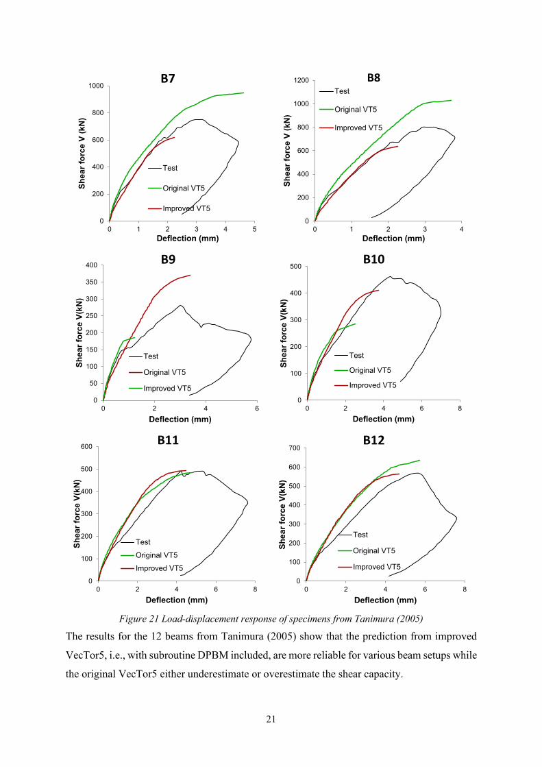
4.1.2 2nd set of tests: Tanimura (2005) The second group of specimens investigated are adopted from Tanimura (2005). These beams
are also under symmetrical 4-point bending as in 4.1.1. The load-displacement response is
shown in Figure 21.
0
500000
1000000
1500000
2000000
2500000
B102 B132 B15 B17 B18Input Time Calc. Time Stiff TimeDecomp Time Invert Time Moca Time
0
500000
1000000
1500000
2000000
2500000
B102 B132 B15 B17 B18Input Time Calc. Time Stiff TimeDecomp Time Invert Time Moca Time

20
0
100
200
300
400
500
600
700
800
900
1000
0 2 4 6 8
Shea
r for
ce V
(kN
)
Deflection (mm)
B1
Test
Original VT5
Improved VT5
0
100
200
300
400
500
600
700
800
900
1000
0 2 4 6
Shea
r for
ce V
(kN
)
Deflection (mm)
B2
Test
Original VT5
Improved VT5
0
100
200
300
400
500
600
700
800
900
1000
0 2 4 6 8
Shea
r for
ce V
(kN
)
Deflection (mm)
B3
Test
Original VT5
Improved VT5
0
200
400
600
800
1000
1200
1400
0 2 4 6 8
Shea
r for
ce V
(kN
)
Deflection (mm)
B4
Test
Original VT5
Improved VT5
0
100
200
300
400
500
600
700
0 1 2 3 4 5
Shea
r for
ce V
(kN
)
Deflection (mm)
B5
Test
Original VT5
Improved VT50
100
200
300
400
500
600
700
800
0 1 2 3 4 5
Shea
r for
ce V
(kN
)
Deflection (mm)
B6
Test
Original VT5
Improved VT5
21
Figure 21 Load-displacement response of specimens from Tanimura (2005)
The results for the 12 beams from Tanimura (2005) show that the prediction from improved
VecTor5, i.e., with subroutine DPBM included, are more reliable for various beam setups while
the original VecTor5 either underestimate or overestimate the shear capacity.
0
200
400
600
800
1000
0 1 2 3 4 5
Shea
r for
ce V
(kN
)
Deflection (mm)
B7
Test
Original VT5
Improved VT50
200
400
600
800
1000
1200
0 1 2 3 4
Shea
r for
ce V
(kN
)
Deflection (mm)
B8Test
Original VT5
Improved VT5
0
50
100
150
200
250
300
350
400
0 2 4 6
Shea
r for
ce V
(kN
)
Deflection (mm)
B9
Test
Original VT5
Improved VT50
100
200
300
400
500
0 2 4 6 8
Shea
r for
ce V
(kN
)
Deflection (mm)
B10
Test
Original VT5
Improved VT5
0
100
200
300
400
500
600
0 2 4 6 8
Shea
r for
ce V
(kN
)
Deflection (mm)
B11
Test
Original VT5
Improved VT50
100
200
300
400
500
600
700
0 2 4 6 8
Shea
r for
ce V
(kN
)
Deflection (mm)
B12
Test
Original VT5
Improved VT5

22
4.2 Continuous deep beam A continuous deep beam was tested in the University of Toronto in 2012 (Mihaylov et al.,
2015), and the details of this beam are shown in Figure 22.
Figure 22 Continuous deep beam specimen
The predicted results from both original VecTor5 and improved VecTor5 as well as the
experimental results are shown in Figure 23. It can be seen the prediction from the improved
VecTor5 is closer to the experimental results compared with the original predictions.
f c= 29.7 MPa f y= 422 MPa ag= 14 mm
0
200
400
600
800
1000
1200
1400
1600
0 2 4 6 8ΔE , mm
East spanP-Test
P-Original VT5
P-Improved VT5
Vint-Test
Vint-Original VT5
Vint-Improved VT5
Vext-Test
Vext-Original VT5
Vext- Improved VT5
P
kN

23
Figure 23 Load-displacement response of specimens from Tanimura (2005)
4.3 Frames
4.3.1 Two-story single-span frame 1) Comparison between predictions from VecTor2 and improved VecTor5
Figure 24 Two-story single-span frame
0
200
400
600
800
1000
1200
1400
1600
0 2 4 6 8 10ΔW, mm
West spanP-Test
P-Original VT5
P-Improved VT5
Vint-Test
Vint-Original VT5
Vint-Improved VT5
Vext-Test
Vext-Original VT5
Vext-Improved VT5
kN
2700
5400
3500
7000
2700
3500
(mm)
3
41 2
3
4
1 2
PP/2 P/2
600
800
2#11
5#11
2#112#115#11
600
1800
4#104#104#10
4#104#104#10
#4@150
#4@250
400
6960
0
3#10
2#10
2#10
3#10
6760
0
300
3#9
3#9
1-1
2-2
3-3
4-4
#4@250
#4@250
69
7115
516
471
155
2x72
=144
692x
72=1
44
3x15
4=46
269
67
40

24
Table 4 Section properties
Section 1-1 Longitudinal reinforcements
φb, mm (#11) 35.81 ≥ 8? yes! As0, mm2 1006
b,mm 600 h,mm 800 Ac,mm2 480000 Asmin, mm2 2400 Asmax, mm2 19200 nb, min 4 nb 16
As, mm2 16096 ≥Asmin? yes! ≤Asmax ? yes!
ρ,% 3.4
c,mm 40 sbmax, mm 152 sb, mm 112 <smax ? yes!
Transverse reinforcements φv, mm (#4) 12.7
Asv0, mm2 129 svmax, mm 573 sv, mm 150 <sv,max? yes!
Section 2-2 Longitudinal reinforcements
φ, mm (#10) 32.26 ≥ 8? yes! As0, mm2 819
b,mm 400 h,mm 600 Ac,mm2 240000 Asmin, mm2 1200 Asmax, mm2 9600 nb, min 4 nb 10
As, mm2 8190 ≥Asmin yes! ≤Asmax yes!
ρ,% 3.4
c,mm 40
sbmax, mm 152 sb, mm 123 <smax? yes!
Transverse reinforcements φv, mm (#4) 12.7
Asv0, mm2 129 svmax, mm 516 sv, mm 150 <sv,max ? yes!
Section 3-3 Longitudinal reinforcements
φ, mm (#10) 32.26
As0, mm2 819 b,mm 600 h,mm 1800 fc, MPa 28 fy,MPa 420 ASTM A615 fu,MPa 620
Ac,mm2 1080000 elongation 7-9% Asmin, mm2 3600 β1 0.85 ρbalance, % 2.85068 ρb, % 1.82 As, mm2 19656 nb 24 c,mm 40 sbmin,mm 25.4 sb, mm
Transverse reinforcements φv, mm (#4) 12.7
Asv0, mm2 svmax, mm sv, mm 250 <sv,max? Yes
Section 4-4 Longitudinal reinforcements
φ, mm (#9) 28.65
As0, mm2 645 b,mm 300 h,mm 600 fc, MPa 28 fy,MPa 420 ASTM A615 fu,MPa 620
Ac,mm2 180000 elongation 7-9% Asmin, mm2 600 β1 0.85 ρbalance, % 2.85068 ρb, % 2.15 As, mm2 3870 nb 6 c,mm 40 sbmin,mm 25.4 sb, mm
Transverse reinforcements φv, mm (#4) 12.7
Asv0, mm2 svmax, mm sv, mm 250 <sv,max? Yes

25
A two-story single-span frame is designed based ACI318_11, and the details are shown in
Figure 24. Point loads are applied on top of the columns with P in themed-column and P/2 in
the two side columns, respectively, simulating the real load case. There is a deep beam in this
frame such that it is necessary to build a mixed-type frame model as shown in Figure 25. In
this model the two shear spans of the deep beam are modelled with Type-8 nonlinear deep
member and the rest are modelled with type-1 nonlinear frame member. It should be noted that
the joints between deep beams and columns are modelled in the same way as suggested in the
original VecTor5: type-1 nonlinear frame members are used within the joint zones and the
steels in the member section are doubled for both longitudinal reinforcement and transverse
reinforcement. Therefore, the deep elements are placed between two joints.
Figure 25 Model of a two-story single-span frame in improved VecTor5
Figure 26 Model of a two-story single-span frame in VecTor2
26
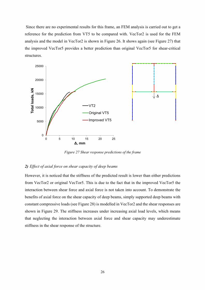
Since there are no experimental results for this frame, an FEM analysis is carried out to get a
reference for the prediction from VT5 to be compared with. VecTor2 is used for the FEM
analysis and the model in VecTor2 is shown in Figure 26. It shows again (see Figure 27) that
the improved VecTor5 provides a better prediction than original VecTor5 for shear-critical
structures.
Figure 27 Shear response predictions of the frame
2) Effect of axial force on shear capacity of deep beams
However, it is noticed that the stiffness of the predicted result is lower than either predictions
from VecTor2 or original VecTor5. This is due to the fact that in the improved VecTor5 the
interaction between shear force and axial force is not taken into account. To demonstrate the
benefits of axial force on the shear capacity of deep beams, simply supported deep beams with
constant compressive loads (see Figure 28) is modelled in VecTor2 and the shear responses are
shown in Figure 29. The stiffness increases under increasing axial load levels, which means
that neglecting the interaction between axial force and shear capacity may underestimate
stiffness in the shear response of the structure.
0
5000
10000
15000
20000
25000
0 5 10 15 20 25
Tota
l loa
ds, k
N
Δ, mm
VT2
Original VT5
Improved VT5
Δ

27
Figure 28 Deep beams used to study the effect of axial force on shear capacity.
Figure 29 Deep beams used to study the effect of axial force on shear capacity.
4.3.2 Two-story two-bay frame The frame in section 4.3.1 is extended to a two-story two-bay frame (see Figure 30). Similarly,
the predictions from original VT5 and improved VT5 are compared in Figure 31.
Figure 30 A two-story two-bay frame
N N
P
0
500
1000
1500
2000
2500
3000
0 4 8 12
V, k
N
Δ, mm
N=0kNN=-350kNN=-700kN
2700
8100
3500
7000
2700
3500
(mm)
3
41 2
3
4
1 2
2700
2 21 1
4
4

28
(a) Deep beam with stirrup ratio ρv=0.65%
(b) Deep beam with stirrup ratio ρv=0.0%
Figure 31 Shear responses predicted with original VecTor5 and improved VecTor5.
4.3.3 Force control vs. displacement control Since all the models mentioned above are loaded in the way of force-control, it is necessary to
check if the improved VecTor5 can carry out displacement-control loading. A third frame is
designed as shown in Figure 32. The results from both force-control loading and displacement-
control loading are plotted in Figure 33. The two results coincide with each other in the pre-
peak range, which means the improved VecTor5 is capable of both force-control and
displacement-control loading.
0
2000
4000
6000
8000
10000
12000
0 10 20 30
Tota
l ver
tical
load
, kN
Vertical displacment at middle column top, mm
ρv=0.65%
Original VT5 (SP=1)
Original VT5 (SP=0)
Improved VT5
0
1000
2000
3000
4000
5000
6000
7000
0 5 10 15
Tota
l ver
tical
load
, kN
Vertical displacment at middle column top, mm
ρv=0.0%
Original VT5 (SP=1)
Original VT5 (SP=0)
Improved VT5

29
Figure 32 A two-story two-bay frame
Figure 33 Shear responses under force-control loading and displacement-control loading.
2700
10600
3500
7000
5200
3500
(mm)
2700
P or disp
0
1000
2000
3000
4000
5000
6000
0 10 20 30
Tota
l ver
tical
load
, kN
Vertical displacment at middle column top, mm
Force-control
Disp-control

30
5 Future Work
5.1 Axial force As mentioned in Section 4.3.1, the interaction between axial force and shear response is not
currently taken into account. Extended formulations should be developed and implemented to
capture this interaction.
5.2 Unloading/reloading paths Attempts were made to include unloading/reloading path for the three springs in the deep beam
element. Due to some numerical problems, these are not included into the implementation.
Future studies should investigate.
5.3 Automatic detection of deep beam elements It could be useful for the user, if an automated algorithm detects all deep beam elements in a
model. Such a feature could be included in future revisions. This work will also require
automatically determining some or all input parameters required by VecTor. DPBM data file.
The ones which could not be determined should still be input by the user.
5.4 Visualization of crack patterns in Janus In Janus, the crack pattern views of deep beam elements have not been implemented.
Undertaking this work will enable in depth visualization of the crack patters and help the user
better interpret the analysis results.
6 References Mihaylov, B.I., Hunt, B., Bentz, E. C. and Collins, M.P. (2015) “Three-parameter kinematic theory for shear behaviour of continuous deep beams,” ACI Structural Journal, 112(1), pp. 47-57. Salamy, M.,R., Kobayashi, H. and Unjoh, S. (2005) “Experimental and analytical study on RC deep beams”, Asian Journal of Civil Engineering (AJCE), 6(5), pp. 409–422. Tanimura, Y. and Sato, T. (2005), “Evaluation of shear strength of deep beams with stirrups”, Quarterly Report of RTRI, 46(1), pp. 53-58. The following is published after the preparation of this report, and contain more refined information.
Liu, J., Guner, S. and Mihaylov, B. (2019) “Mixed-Type Modeling of Structures with Slender and Deep Beam Elements” ACI Structural Journal, 116(4), pp. 253-264. <web link>

31
Annex 1: Flow chart of subroutine DPBM


