JOURNAL OF THE OPTICAL SOCIETY OF AMERICA VOLUME 33 NUMBER 5 MAY, 1943

A Metric for Colorspace* PARRY MOON, Massachusetts Institute of Technology, Cambridge, Massachusetts

AND

DOMINA EBERLE SPENCER, The American University, Washington, D. C.

1. INTRODUCTION

TH E familiar C.I .E. system of color specifica­tion is based on experiments wi th exact

color matches . I t s geometric representation is an affine space in which, as in any affine space, angles and distances cannot in general be compared. I t is na tura l for the colorimetrist to inquire if addi­tional information can be obtained by introduc­ing a metr ic into the affine colorspace. Helm-holtz1 was the first to take such a step, and he identified the metr ic with minimum perceptible color difference. If a successful metr ic can be established, it will widen the scope of the C.I .E. colorspace by giving a geometric representation to all available information on color discrimina­tion. Considerable previous effort has been de­voted to the subject, wi thout , however, leading to any completely satisfactory solution.

T h e present paper develops a metr ic for color-space. T h e method employs non-linear t rans­formations in place of the linear t ransformations ordinarily used; and the conclusions are based on experimental results ra ther than on speculations. In presenting this material , we first give an ele­menta ry outline of the basic mathemat ica l ideas. Such an outline would be superfluous for ma the ­maticians b u t may prove helpful to colorime-trists. A metr ic is then introduced in a plane of constant helios,2, 3 after which it is extended to the color 3 space.

T h e Riemannian metric is wri t ten

(1) may be regarded as the definition of a quan­t i ty ds by which distances are determined be­tween pairs of points in the coordinate space.

If the coordinate surfaces are orthogonal, Eq . (1) becomes

For the special case where the metr ic coefficients are all uni ty, the Euclidean metric is obtained:

When the Euclidean metric is introduced into an affine space, the space becomes the familiar space of elementary geometry.

T h e ordinary affine colorspace can be changed to a metr ic space by introducing any metric t h a t the investigator desires. There is nothing in the C.I .E. d a t a to indicate wha t metr ic is to be used, nor do philosophical speculations lead to any­thing of value. The metric coefficients must be obtained by consideration of additional experi­mental data. Available da t a are of two kinds: color discrimination taken a t constant helios, and contras t sensitivity obtained a t constant chromatici ty .

Consider a region of space about a given point P , the region being so small t ha t the metr ic co­efficients can be considered as constants . We in­quire as to the shape of the surface ∆s = 1, which lies in the foregoing restricted region of space. T h e equation of the surface is, according to Eq. (1),

where dxi and dxl are elementary distances along any three coordinate axes. T h e metric coefficients gij may be constants or they may be arb i t ra ry functions of the coordinates x1, x2, x3. Equat ion

* Based on a paper presented by one of the authors at the annual meeting of the Optical Society of America, New York, October 31, 1942.

1 H. v. Helmholtz, Berlin Akad. Sci. 1071 (1891). Hand-buch der physiologischen Optik (Leipzig, 1896), second edition.

2 Parry Moon, J. Opt. Soc. Am. 32, 348 (1942). 3 D. E. Spencer, J. Opt. Soc. Am. 33, 10 (1943).

where the g's are constants . Bu t this is the equa­tion of an ellipsoid.** T h e principal axes of the

** Equation (4) represents a quartic surface. However, in this application it must be a quartic surface that re­mains finite and hence an ellipsoid.

260

A M E T R I C FOR C O L O R S P A C E 261

ellipsoid are generally not in the directions of the coordinate axes. But if the coordinate axes are axes of symmetry of the ellipsoid, Eq. (4) be­comes

l /g1 1 , l/g22, and l/g33 are the lengths of the semi-axes of the ellipsoid if the coordinate axes are orthogonal with respect to this metric.

Thus by rotation of the coordinate axes until they are orthogonal and are parallel to the prin­cipal axes of the ellipsoid, any particular ellip­soid can be represented by the foregoing simple equation. The surface of colors that are just per­ceptibly different from a given color P is then an ellipsoid having its principal axes in the direction of the coordinate axes and its center at P. The three axes of the ellipsoid are generally different because g11 , g22 , and g33 are not the same.

Any colorspace can be made locally Euclidean. But the metric coefficients will generally be differ­ent at two distinct points P and Q. Thus if the ellipsoid at P is transformed into a sphere, the one at Q will ordinarily remain an ellipsoid. In the special case in which a single transformation of variables eliminates the cross products for all points in space, Eq. (4) becomes

A Euclidean metric is possible for the whole space if the following new variables can be intro­duced :

In general, however, no such simplicity obtains and no Euclidean metric is possible.

2. A METRIC IN A PLANE OF CONSTANT HELIOS

One method of introducing a metric into color-space is to assume a Euclidean metric and to find what linear transformation of the C.I.E. space will give a reasonable approximation to the ex­perimental data on color discrimination. This method is obviously doomed to failure in the 3 space since it gives no approximation to the well-established effect of helios variation. In the 2

space, however, it can be put in reasonably good agreement with experiment. Judd4 was the first to use a projective transformation of the C.I.E. chromaticity diagram in an attempt to find a metric, and the resulting Maxwell triangle was found to give fairly good agreement with most experimental results on color discrimination. Other projective transformations giving similar results have been originated by MacAdam,5

Breckenridge and Schaub,6 Sinden,7 and Adams.8

The present paper differs from its predecessors in using non-linear transformations, and it will be shown that the resulting 2 space has ad­vantages over the others.

Numerous researches have been conducted on the minimum perceptible color variation at con­stant helios, or on related quantities. The most recent investigation is that of MacAdam9 who kept the helios of the test spots at a value of 150 blondels and who employed a surround having half this helios.2 Illuminant C was used in lighting the surround. Twenty-five points were taken in the color 2 space. For each point, color matches were made along a number of lines in the chro­maticity diagram; and for each line the standard deviation of the results was computed. I t was found that the standard deviation determined an ellipse about the chosen point.

When the MacAdam ellipses are plotted in the C.I.E. chromaticity diagram9 (Fig. 1), they are found to be of different sizes and orientations so that no Euclidean metric can be employed in this diagram. To obtain values of the metric coeffi­cients g11 , g13 , and g33 of Eq. (1), we replotted the ellipses in the plane of constant helios, Y=150, using the equations,

The surprising result was that the major axes of the ellipses became essentially parallel. In fact, the MacAdam data can be fitted by a set of ellipses with major axes having the slope in the XZ plane of +4.32. These ellipses are shown in

4 D. B. Judd, J. Opt. Soc. Am. 25, 24 (1935); J. Research Nat. Bur. Stand. 14, 41 (1935).

5 D. L. MacAdam, J. Opt. Soc. Am. 27, 294 (1937). 6 Breckenridge and Schaub, J. Opt. Soc. Am. 29, 370

(1939). 7 R. H. Sinden, J. Opt. Soc. Am. 27, 124 (1937); 28, 339 (1938).

8 E. Q. Adams, J. Opt. Soc. Am. 32, 168 (1942). 9 D. L. MacAdam, J. Opt, Soc Am, 32, 247 (1942),

262 P A R R Y M O O N A N D D . E . S P E N C E R

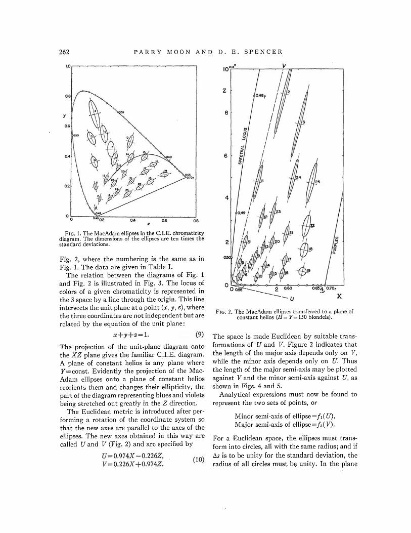
FIG. 1. The MacAdam ellipses in the C.I.E. chromaticity diagram. The dimensions of the ellipses are ten times the standard deviations.

Fig. 2, where the numbering is the same as in Fig. 1. The data are given in Table I.

The relation between the diagrams of Fig. 1 and Fig. 2 is illustrated in Fig. 3. The locus of colors of a given chromaticity is represented in the 3 space by a line through the origin. This line intersects the unit plane at a point (x, y, z), where the three coordinates are not independent but are related by the equation of the unit plane:

The projection of the unit-plane diagram onto the XZ plane gives the familiar C.I.E. diagram. A plane of constant helios is any plane where Y= const. Evidently the projection of the Mac-Adam ellipses onto a plane of constant helios reorients them and changes their ellipticity, the part of the diagram representing blues and violets being stretched out greatly in the Z direction.

The Euclidean metric is introduced after per­forming a rotation of the coordinate system so that the new axes are parallel to the axes of the ellipses. The new axes obtained in this way are called U and V (Fig. 2) and are specified by

FIG. 2. The MacAdam ellipses transferred to a plane of constant helios (H= Y= 150 blondels).

The space is made Euclidean by suitable trans­formations of U and V. Figure 2 indicates that the length of the major axis depends only on V, while the minor axis depends only on U. Thus the length of the major semi-axis may be plotted against V and the minor semi-axis against U, as shown in Figs. 4 and 5.

Analytical expressions must now be found to represent the two sets of points, or

Minor semi-axis of ellipse =f1 (U), Major semi-axis of ellipse =ƒ3(V).

For a Euclidean space, the ellipses must trans­form into circles, all with the same radius; and if As is to be unity for the standard deviation, the radius of all circles must be unity. In the plane

A M E T R I C F O R C O L O R S P A C E 263

of constant helios, therefore, the metric is

The UV plane is transformed into a plane in which the metric is Euclidean,

where

Thus the equations for the transformations are

treme violet of the spectral locus is at V= 26,000. No data are available in the intervening region; so a number of equations can be used for ƒ3(V) which will fit the data equally well but which will behave differently at large values of V. The first equation tried was

which is in excellent agreement with the data except for Ellipses 1 and 2 (Table I). The new

where C1 and C3 are constants of integration. Evidently neither set of data (Fig. 4 or 5) can

be represented by a linear function, so no pro­jective transformation5 of the C.I.E. chromaticity diagram will adequately represent the experi­mental evidence. The data of Fig. 4, however, are fitted very well by the parabola:

In fact, no other satisfactory expression for f1 (U) has been found.

For the data of Fig. 5, however, the MacAdam ellipses extend to only V=2100 while the ex-

TABLE I. Ellipses in a plane of constant helios (H =150 blondels).

FIG. 3. Three-dimensional representation showing the relation between the chromaticity diagram and a plane of constant helios.

coordinates, according to Eq. (14), are

The spectral locus shows a point of inflection in the ξ diagram and is found to be concave from about 0.40 to 0.50μ. This characteristic is rather startling, since in previous diagrams the locus has always been convex.4 In fact, it is easy to prove that the convexity of the spectral locus is an affine invariant. Though there appears to be no a priori reason why the same should be true in the ξ diagram, we thought it advisable to investi­gate the possibility of a convex locus. Accord­ingly, various transformations were considered,

264 PARRY MOON AND D. E. SPENCER among which may be mentioned: denominator may be altered through a consider­

able range without change in the other constants. Until more complete data at short wave-lengths are available, however, this additional refinement appears to be unnecessary. From a study of the various transformations, we have reached the conclusion that a concavity of the spectral locus cannot be avoided in the ξ diagram except by modification of either the MacAdam data or the C.I.E. trichromatic data.

On the basis of available data, therefore, we recommend the use of Eq. (21). The metric coefficients are:

These equations are in equally good agreement with the MacAdam ellipses but result in different behavior of the spectral locus in the ξ diagram from 0.40 to 0.50μ.

Equations (18) and (19) move the violet end of the spectrum to very high values of ξ3, which is not in agreement with data on the number of steps from white to the spectral locus.10 Some of the other equations are inconvenient. The best one appears to be Eq. (21). It still gives a slight concavity of the locus, but it agrees with all the MacAdam ellipses (including Nos. 1 and 2) and it appears to be in reasonable agreement with all other pertinent data. Equation (22) may also be used, and the coefficient of the final term in the

The transformations to the ξ diagram are:

The constants Cl and C3 are entirely arbitrary. The simplest transformation is obtained by mak-

FIG. 4. Minor semi-axes of the MacAdam ellipses in the plane Y= 150.

10 Martin, Warburton, and Morgan, Med. Res. Council Report, London (1933).

FIG. 5. Major semi-axes of the MacAdam ellipses in the plane Y= 150.

A M E T R I C F O R C O L O R S P A C E 265

FIG. 6. MacAdam ellipses transferred to the ξ1ξ3 diagram. All the ellipses become circles of equal size. The numbering agrees with that of Fig. 1.

ing them both zero, as will be done in this paper. There is a slight advantage for some purposes in placing the center of coordinates at an achro­matic point, in which case the different quadrants contain related colors much as in the Brecken-ridge diagram.6

Use of Eq. (24) results in the peculiar prow-shaped diagram of Fig. 6. The curve of saturated purples was obtained by taking 10 equally-spaced points between the extremes of the spectral locus in the C.I.E. chromaticity diagram. The result is not a straight line because of the non-linear trans­formation of Eq. (24). The transformed Mac-Adam ellipses are now circles, all with unit radius. The dimensions of these circles in Fig. 6 are made ten times their true values, as was done with the original ellipses (Fig. 1). The numerical designa­tion of the MacAdam circles also agrees with that of Fig. 1.

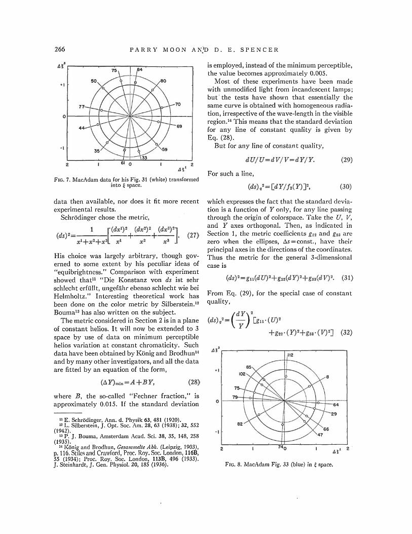
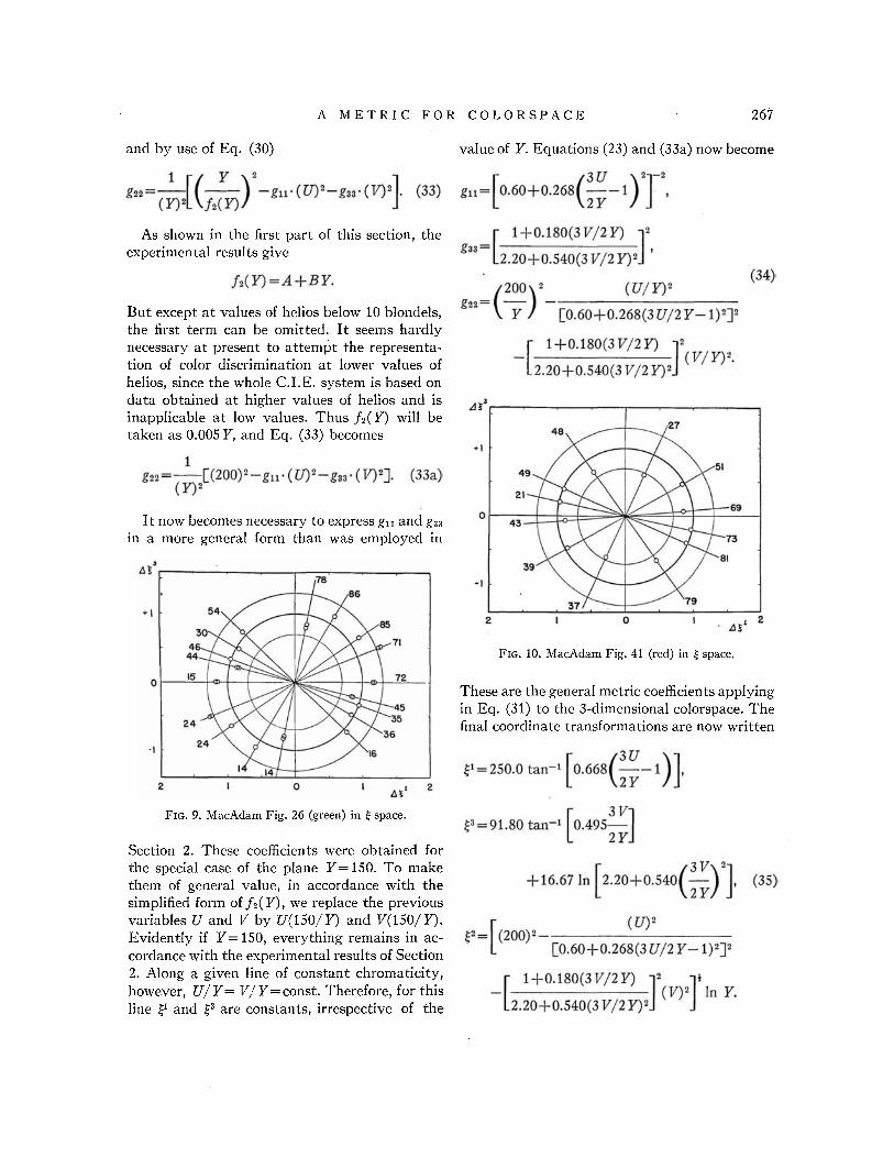
Typical transformed ellipses are shown in Figs. 7, 8, 9, and 10. The dots are the MacAdam experi­mental points, transformed by means of Eq. (24). These points are in reasonably good agreement with the heavy circles having unit radius. Light circles having radii which differ by ± 3 0 percent from the heavy circles indicate the approximate limits of scatter of the experimental data. In some cases the points seem to indicate an ellip-ticity, but it is doubtful if this appearance has

any validity. Note that the wide variations in size and shape, shown in Figs. 1 and 2, have dis­appeared. The other MacAdam circles are not shown, in order to save space. However, within the limits of experimental error, all of the data are representable by unit circles.

3. A METRIC IN 3 SPACE

Helmholtz1 based his metric on experimental results in 1 space (variation of helios only), which gave

He considered as a "probable hypothesis" that the extension to 3 space would give

where xi are the amounts of the "physiologischen Urfarben" and ai are constants. This provides a Euclidean metric in the variables ξi, where

Because of the scarcity of experimental data, there was little that Helmholtz could do except make a reasonable guess such as Eq. (25). His metric, however, did not agree with the König

P A R R Y MOON A N D D. E. S P E N C E R

is employed, instead of the minimum perceptible, the value becomes approximately 0.005.

Most of these experiments have been made with unmodified light from incandescent lamps; but the tests have shown that essentially the same curve is obtained with homogeneous radia­tion, irrespective of the wave-length in the visible region.14 This means that the standard deviation for any line of constant quality is given by Eq. (28).

But for any line of constant quality,

FIG. 7. MacAdam data for his Fig. 31 (white) transformed into ξ space.

For such a line,

data then available, nor does it fit more recent experimental results.

Schrödinger chose the metric,

His choice was largely arbitrary, though gov­erned to some extent by his peculiar ideas of "equibrightness." Comparison with experiment showed that11 "Die Konstanz von ds ist sehr schlecht erfüllt, ungefähr ebenso schlecht wie bei Helmholtz." Interesting theoretical work has been done on the color metric by Silberstein.12

Bouma13 has also written on the subject. The metric considered in Section 2 is in a plane

of constant helios. It will now be extended to 3 space by use of data on minimum perceptible helios variation at constant chromaticity. Such data have been obtained by König and Brodhun14

and by many other investigators, and all the data are fitted by an equation of the form,

which expresses the fact that the standard devia­tion is a function of Y only, for any line passing through the origin of colorspace. Take the U, V, and Y axes orthogonal. Then, as indicated in Section 1, the metric coefficients g12 and g23 are zero when the ellipses, ∆s = const., have their principal axes in the directions of the coordinates. Thus the metric for the general 3-dimensional case is

From Eq. (29), for the special case of constant quality,

where B, the so-called "Fechner fraction," is approximately 0.015. If the standard deviation

11 E. Schrödinger, Ann. d. Physik 63, 481 (1920). 12 L. Silberstein, J. Opt. Soc. Am. 28, 63 (1938); 32, 552

(1942). 13 P. J. Bouma, Amsterdam Acad. Sci. 38, 35, 148, 258

(1935). 14 König and Brodhun, Gesammelte Abh. (Leipzig, 1903),

p. 116. Stiles and Crawford, Proc. Roy. Soc. London, 116B, 55 (1934); Proc. Roy. Soc. London, 113B, 496 (1933). J. Steinhardt, J. Gen. Physiol. 20, 185 (1936). FIG. 8. MacAdam Fig. 33 (blue) in ξ space.

266

A M E T R I C FOR C O L O R S P A C E 267

and by use of Eq. (30) value of F. Equations (23) and (33a) now become

As shown in the first part of this section, the experimental results give

But except at values of helios below 10 blondels, the first term can be omitted. It seems hardly necessary at present to attempt the representa­tion of color discrimination at lower values of helios, since the whole C.I.E. system is based on data obtained at higher values of helios and is inapplicable at low values. Thus f2(Y) will be taken as 0.005 Y, and Eq. (33) becomes

It now becomes necessary to express g11 and g33 in a more general form than was employed in

F I G . 10. MacAdam Fig. 41 (red) in ξ space.

These are the general metric coefficients applying in Eq. (31) to the 3-dimensional colorspace. The final coordinate transformations are now written

F I G . 9. MacAdam Fig. 26 (green) in ξ space.

Section 2. These coefficients were obtained for the special case of the plane F=150. To make them of general value, in accordance with the simplified form of ƒ2(Y), we replace the previous variables U and V by U(150/Y) and V(150/Y). Evidently if F=150, everything remains in ac­cordance with the experimental results of Section 2. Along a given line of constant chromaticity, however, U/Y= V/Y= const. Therefore, for this line ξl and ξ3 are constants, irrespective of the

268 PARRY MOON AND D. E. SPENCER

F I G . 11. The ξ1ξ3 diagram showing spectral locus, line of saturated purples, and Planckian locus.

Here Y=H= helios, expressed in blondels, and U and V are obtained from Eq. (10).

Equation (35) shows that the ξ1ξ3 diagram is exactly the same for any value of helios. Thus whenever interest is in chromaticity only and the helios is constant, the ξ1ξ3 diagram plays a role similar to that of the familiar C.I.E. chromaticity diagram. The ξ diagram is shown again in Fig. 11 with the Planckian locus included. All informa­tion on color discrimination at constant helios, such as minimum perceptible wave-length differ­ence along the spectral locus, can be obtained directly from the diagram. If helios variation is also encountered, the 3 space is used (Fig. 12). The surfaces ∆s = l are spheres of the same size throughout the ξ space, and the spectral locus is a cylinder. Distances between points have the same significance as in the 2 space.

related to the C.I.E. coordinates by elementary (though non-linear) functional transformations. The familiar C L E . affine colorspace is trans­formed into a three-dimensional ξ space in which minimum perceptible color differences are repre­sented by small spheres of the same size through­out the space. Geodesies are straight lines, and all the other properties of elementary Euclidean geometry apply directly in this new colorspace.

Planes of constant helios in the C.I.E. space transform into planes in the ξ space. All of these ξ1ξ3 diagrams are identical and give a Euclidean representation of the C.I.E. chromaticity dia­gram. It can be shown that the new 2 space is in

4. SUMMARY

The paper develops a new metric for color-space. It is found that, within the limits of experi­mental error, data on color discrimination can be fitted by the Euclidean metric,

where ξ1, ξ2, and ξ3 are new coordinates which are FIG, 12. The thres dimensional ξ space.

B O O K R E V I E W 269

supplements it. Colors are first specified in terms of X, Y, and Z; and these values can then be transformed into ξ1, ξ2, and ξ3. The ξ space has many advantages, but these advantages have been obtainable only by giving up the simple geometric representation of addition. The addi­tion of two colors cannot be obtained vectorially in ξ space, and straight lines in the C.I.E. space are transformed into curves in the new space.

better accord with experimental data than has been obtained with the projective transforma­tions, which were developed previously.5

The new ξ space has important applications in colorimetry and gives for the first time a mathe­matical method of comparing colors which differ both in quality and quantity. It should be em­phasized, however, that the new system does not in any way replace the C.I.E. system but only