Download - A Guide to Tracking the U.S. Economy models cannot predict. Second, most key data used to measure the economy and track its performance are often revised—and by substantial amounts

Federal Reserve Bank of St. Louis REVIEW First Quarter 2014 35

A Guide to Tracking the U.S. Economy

Kevin L. Kliesen

Analyzing and forecasting the performance of the U.S. and global economies is a daunt-ing challenge, even for trained, professional economists. This means the challengefacing the nonpractitioner is probably much more difficult. For example, suppose a

furniture retailer would like to know the direction of interest rates and the unemploymentrate over the next year or two. The direction of interest rates is important because sales ofdurable goods such as furniture tend to be interest rate sensitive. Likewise, if an increasingpercentage of the labor force becomes unemployed, then sales will tend to suffer. But othereconomic variables are also important. Household wealth, home sales, and consumer senti-ment are often used by forecasters and some monetary policymakers to help predict thefuture path of consumer spending on durable goods.

If the retailer guesses wrong and orders too much or too little furniture from the factory,this may lead to either too much or too little inventory on hand. If too much furniture isordered, the retailer’s costs of carrying the extra inventory would increase, whereas if too littleis ordered, the retailer’s sales might suffer. In both instances, the retailer’s profits would prob-ably be reduced relative to what was expected. In short, a furniture retailer has a powerfulincentive to form some assessment of the economy’s future performance.

Analyzing and forecasting the performance and direction of a large, complex economy like that ofthe United States is a difficult task. The process involves parsing a great deal of data, understandingkey economic relationships, and assessing which events or factors might cause monetary or fiscalpolicymakers to change policy. One purpose of this article is to reinforce several key principles thatare useful for tracking the U.S. economy’s performance in real time. Two principles stand out: First,the economy is regularly hit by unexpected economic disturbances (shocks) that policymakers andforecasting models cannot predict. Second, most key data used to measure the economy and track itsperformance are often revised—and by substantial amounts. (JEL E32, E66)

Federal Reserve Bank of St. Louis Review, First Quarter 2014, 96(1), pp. 35-54.

Kevin L. Kliesen is a research officer and economist at the Federal Reserve Bank of St. Louis. Douglas C. Smith and Lowell R. Ricketts providedresearch assistance.

© 2014, The Federal Reserve Bank of St. Louis. The views expressed in this article are those of the author(s) and do not necessarily reflect the viewsof the Federal Reserve System, the Board of Governors, or the regional Federal Reserve Banks. Articles may be reprinted, reproduced, published,distributed, displayed, and transmitted in their entirety if copyright notice, author name(s), and full citation are included. Abstracts, synopses, andother derivative works may be made only with prior written permission of the Federal Reserve Bank of St. Louis.

http://research.stlouisfed.org/econ/kliesen/

This article is not a how-to exercise in building economic models. Rather, it is intendedto assist the noneconomist (nonpractitioner) who wants to analyze and interpret patterns ofeconomic activity at the macro level. A nonpractitioner can be a businessperson, an investor,or any individual interested in monitoring the U.S. economy and/or developing an expectationof its short-term direction. A key conclusion is that the economy’s performance can changerapidly. Accordingly, the nonpractitioner seeking some clues about the short-term directionof the economy is advised to monitor a handful of key data and then balance this informationagainst freely available consensus forecasts of the economy over the next six months or so.Over time, consensus forecasts, which are simple averages of a group of professional forecasters,tend to be more accurate than any individual forecast.

A BASIC MODEL OF ECONOMIC FLUCTUATIONSA practicing forecaster usually needs a model of how the macroeconomy works. For pro-

fessional forecasters, the “model” is usually a sophisticated system of equations designed toexplain key aspects of the economy—such as growth of real gross domestic product (GDP),inflation, interest rates, stock prices, and the unemployment rate. Nonpractitioners—thosenot actively managing a large econometric forecasting model—tend to be at a distinct disad-vantage in this domain. To compensate, the nonpractitioner who needs to make some judg-ment about the future direction of the economy should adopt a less formal economic model.Such a model would convey a broad notion of how the economy evolves over the businesscycle. One simplistic model the nonpractitioner can use to organize his or her thoughts wouldbe the following: U.S. economic activity—or real GDP—revolves around a trend that growsroughly at a rate determined by the sum of labor productivity growth and population growth.1This trend is sometimes called the growth rate of the economy’s potential output. Deviationsaround this trend—termed “economic fluctuations”—occur because of unexpected distur-bances (termed “shocks”), new technologies, and the ever-evolving preferences of consumers,firms, and government policymakers to save, spend, and regulate.

With this simplistic model, the nonpractitioner can make reasonably accurate assessmentsabout the likely direction of the economy over the next several months or quarters. For exam-ple, if auto and home sales are strengthening, the unemployment rate is falling, job gains arepicking up, and stock prices are rising, then these factors are usually reliable signals that theeconomy is on an upswing. The nonpractitioner should thus exploit the fact that many key vari-ables move together, which is known as comovement (see the boxed insert on the next page).Comovement is important because the economy’s natural state is one of positive growth—where this growth is dependent on the economy’s fundamentals. At any point in time, then,the economy will be growing above or below this trend rate of growth, which will then affectimportant variables such as, inflation, interest rates, and the unemployment rate.2

A model of inflation also differentiates between short- and long-run movements. Inflationcan vary over shorter periods of time with changes in energy prices or labor costs. However,over longer periods (several years), actions taken by monetary policymakers will have a sig-nificant influence on the economy’s inflation rate. Importantly, this transmission stems from

Kliesen

36 First Quarter 2014 Federal Reserve Bank of St. Louis REVIEW

Kliesen


Exploit the Principle of Comovement

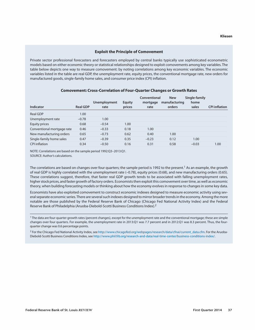
Private sector professional forecasters and forecasters employed by central banks typically use sophisticated econometricmodels based on either economic theory or statistical relationships designed to exploit comovements among key variables. Thetable below depicts one way to measure comovement: by noting correlations among key economic variables. The economicvariables listed in the table are real GDP, the unemployment rate, equity prices, the conventional mortgage rate, new orders formanufactured goods, single-family home sales, and consumer price index (CPI) inflation.

Comovement: Cross-Correlation of Four-Quarter Changes or Growth Rates

Conventional New Single-family Unemployment Equity mortgage manufacturing home

Indicator Real GDP rate prices rate orders sales CPI inflation

Real GDP 1.00Unemployment rate –0.78 1.00Equity prices 0.68 –0.54 1.00Conventional mortgage rate 0.46 –0.33 0.18 1.00New manufacturing orders 0.65 –0.73 0.62 0.40 1.00Single-family home sales 0.47 –0.39 0.35 –0.23 0.12 1.00CPI inflation 0.34 –0.50 0.16 0.31 0.58 –0.03 1.00

NOTE: Correlations are based on the sample period 1992:Q3–2013:Q1.SOURCE: Author’s calculations.

The correlations are based on changes over four quarters; the sample period is 1992 to the present.1 As an example, the growthof real GDP is highly correlated with the unemployment rate (–0.78), equity prices (0.68), and new manufacturing orders (0.65).These correlations suggest, therefore, that faster real GDP growth tends to be associated with falling unemployment rates,higher stock prices, and faster growth of factory orders. Economists then exploit this comovement over time, as well as economictheory, when building forecasting models or thinking about how the economy evolves in response to changes in some key data.

Economists have also exploited comovement to construct economic indexes designed to measure economic activity using sev-eral separate economic series. There are several such indexes designed to mirror broader trends in the economy. Among the morenotable are those published by the Federal Reserve Bank of Chicago (Chicago Fed National Activity Index) and the FederalReserve Bank of Philadelphia (Aruoba-Diebold-Scotti Business Conditions Index).2

1 The data are four-quarter growth rates (percent changes), except for the unemployment rate and the conventional mortgage; these are simplechanges over four quarters. For example, the unemployment rate in 2013:Q1 was 7.7 percent and in 2012:Q1 was 8.3 percent. Thus, the four-quarter change was 0.6 percentage points.2 For the Chicago Fed National Activity Index, see http://www.chicagofed.org/webpages/research/data/cfnai/current_data.cfm. For the Aruoba-Diebold-Scotti Business Conditions Index, see http://www.phil.frb.org/research-and-data/real-time-center/business-conditions-index/.

the effects of these policy actions on the market’s expectations about future inflation. WilliamPoole (2005, pp. 303-04), former president of the Federal Reserve Bank of St. Louis, provideda nice summary of how this might work in practice:

My sense of what I do, which I think is not dissimilar to what most FOMC [Federal Open MarketCommittee] members do, is attempt to intuit future inflation pressures from current observedpressures as they show up in both price changes and resource pressures, or real gaps, in individualmarkets. The approach is not totally without theory; for example, wage changes are evaluated inlight of expected productivity trends. I attempt to sort out temporary from more lasting wageand price changes and attempt informally to construct an appropriately weighted average of dis-parate experience in various sectors. I look closely at data on inflation expectations, but treat suchdata carefully because longer-run expectations are really a vote of confidence on the Fed and notan independent reading on inflation.

I am extremely uncomfortable with this approach and believe that it is an invitation to futuremistakes. I don’t know what better to do.

The nonpractitioner faces another key disadvantage relative to professional forecasters oreconomic policymakers: resource constraints. Thus, returning to our earlier example, smallfirms tend to be at a disadvantage compared with large firms in trying to analyze the directionof the economy. Large firms have the resources to hire economists to sift through the data andconstruct their own sophisticated forecasting models, or they can benefit from professionalforecasting services on a contract basis. To help offset this disadvantage, a small business ownerwill probably adopt some form of naive forecasting (“what happened last year will happenagain this year”) by reading economic and financial market commentaries from trade associa-tions or perusing “reputable” economic blogs. Some may also use common rules of thumbpurported to gauge the strength and direction of the economy, such as the direction of thestock market.

The challenge of economic forecasting extends beyond the technical expertise requiredto make accurate forecasts. Other factors contributing to this difficult task include the sheervolume of data, persistent data revisions, and correct interpretation of data that may sendconflicting signals. Other complications are the responses of monetary and fiscal policymakersand foreign economic developments. Before expounding on how a nonpractitioner might tryto overcome these challenges, the next section offers a brief discussion of the events leadingup to 2008. The so-called Financial Panic of 2008 and the Great Recession offer several exam-ples of the difficulties both nonpractitioners and professional forecasters face as they attemptto learn about the direction of the economy and forecast its short-term future path.

THE PERILS OF FORECASTING: A LOOK BACK AT 2008The late economist John Kenneth Galbraith reportedly once remarked that there are

two types of forecasters: those who don’t know and those who don’t know they don’t know.Galbraith’s aphorism reveals an underappreciated aspect of forecasting: It is inherently diffi-cult. Thus, it was not surprising that the onset of the recent recession was not foreseen by themajority of the professional forecasting community. According to the Business Cycle Dating

Kliesen


Committee of the National Bureau of Economic Research (NBER), the U.S. economic expan-sion that began in November 2001 ended sometime in December 2007.3 However, by the endof 2007, very few professional forecasters were predicting a recession in 2008. In fact, in theDecember 2007 Blue Chip Economic Indicators, the consensus of the Blue Chip forecasterswas that real GDP would increase by 2.2 percent in 2008. The average of the 10 most pessimis -tic forecasters was 1.6 percent, while the average of the 10 most optimistic forecasters was2.7 percent.4

The NBER Business Cycle Dating Committee, like many nonpractitioners, tends to lookat real GDP as a key indicator (among other indicators) of the economy’s performance. Forexample, increases (decreases) in expenditures for real final goods and services—such as auto-mobiles, refrigerators, or physician services—are regularly followed by increases (decreases)in employment and a lower (higher) unemployment rate. As Figure 1 shows, throughoutmost of 2007 the Blue Chip Consensus (BCC) of professional forecasters was that real GDPwould increase by about 3 percent in 2008. This figure plots a timeline of BCC forecasts forreal GDP growth in 2008. The first forecast was published in January 2007. Beginning inSeptember 2007, though, forecasters began to steadily lower their projections for real GDPgrowth in 2008. In particular, as discussed below, the forecasts for real GDP growth for 2008turned sharply lower after the widespread financial turmoil in September 2008. By the end ofNovember 2008, when the NBER announced that the recession began sometime in December2007, the BCC forecast for real GDP growth in 2008 had dipped slightly below zero.

Kliesen


–0.2Initial Actual

–3.3Current Estimate

–4.0

–3.0

–2.0

–1.0

0

1.0

2.0

3.0

4.0

Jan. 2007 Jul. 2007 Jan. 2008 Jul. 2008 Jan. 2009 Jul. 2009

2008 (Real GDP)December 2007September 2008

Percent (Annual Rate)

Figure 1

A Timeline of Blue Chip Forecasts for Real GDP Growth in 2008

SOURCE: Blue Chip Economic Indicators, various issues.

The direction of inflation is another key indicator of economic performance. First, long-term interest rates such as mortgage rates and corporate bond yields have an inflation pre-mium.5 Accordingly, if inflation or the perceived risk of higher inflation in the future increases,then interest rates also usually rise. A higher inflation rate may also spur the Fed to raise itsshort-term interest rate target, which could also cause long-term rates to rise.6 The directionof inflation was markedly different over a good portion of this period. As Figure 2 shows, fromJanuary 2007 until March 2008, the BCC forecast was that the CPI would increase by a bit lessthan 2.5 percent in 2008.

The relative stability of inflation expectations was somewhat surprising given the behaviorof oil prices and actual inflation over this period. From January 2007 to March 2008, crudeoil prices rose from about $55 per barrel to about $106 per barrel. Over the same period, theyear-to-year percent change in the CPI rose from 2.1 percent to 4 percent. As oil prices andactual inflation continued to rise over the first half of 2008, forecasters began to dramaticallyraise their forecasts for inflation in 2008—from about 2.75 percent in April to 4.5 percent inSeptember.7 Interestingly, though, forecasts for CPI inflation in 2009 (not shown) rose onlyslightly, which suggests that most forecasters tended to believe that the upsurge in inflation in2008 would be temporary. This forecast proved to be accurate. (See the boxed insert on p. 46.)

A key takeaway message from Figures 1 and 2 is that significant, unexpected economicshocks can have important effects on the expectations of forecasters—and thus investors andeconomic policymakers. The remainder of the article discusses a methodology the nonprac-

Kliesen


0

0.5

1.0

1.5

2.0

2.5

3.0

3.5

4.0

4.5

5.0

Percent (Annual Rate)

Jan. 2007 Jul. 2007 Jan. 2008 Jul. 2008 Jan. 2009 Jul. 2009

1.6Actual

2008 (CPI In!ation)December 2007September 2008

Figure 2

A Timeline of Blue Chip Forecasts for CPI Inflation in 2008

SOURCE: Blue Chip Economic Indicators, various issues.

titioner can use to help analyze the current and short-term performance of the U.S. economy.This approach relies on publicly available data and macroeconomic forecasts. In this frame-work, “reading the tea leaves” requires an assessment of the following economic conditions:

• the economy’s momentum (slowing or accelerating); • the headwinds or tailwinds affecting this momentum and how long they are expected

to last; and• the risks to the outlook—that is, what could produce growth that is either faster or

slower than expected for economic activity and prices.

Endnotes are used for those seeking references or a more in-depth discussion about analyz-ing general business conditions and the macroeconomy. Although the U.S. economy is obvi-ously affected by events in other countries, the discussion focuses primarily on U.S. data flowsand the decisions adopted by U.S. economic policymakers and their potential economicconsequences.

KEY PRINCIPLES FOR TRACKING THE ECONOMYPrinciple #1: Use Freely Available Forecasts

The nonpractitioner should adhere to a set of key economic principles. One such princi-ple is comparative advantage. That is, the nonpractitioner should use forecasts developed byprofessional economists with advanced training and experience in modeling and forecasting.Another principle pertains to the law of demand, which relates the price of a good to itsquantity demanded: Free is usually better. Fortunately, reputable forecasts are freely available

Kliesen


Table 1

Free Economic Forecasts

Name Source Frequency URL

Survey of Professional Federal Reserve Bank Quarterly http://www.phil.frb.org/research-and-data/Forecasters of Philadelphia real-time-center/survey-of-professional-

forecasters/

FOMC Summary of Federal Open Quarterly http://www.federalreserve.gov/monetarypolicy/Economic Projections Market Committee fomccalendars.htm

IMF World Economic International Semiannually http://www.imf.org/external/ns/cs.aspx?id=29Outlook Reports Monetary Fund

NABE Outlook (partial) National Association Quarterly http://nabe.com/NABE_Outlook_Summaryfor Business Economics

Budget and Economic Congressional Annually http://www.cbo.gov/publication/43907Outlook Budget Office

Economic Outlook OECD Semiannually http://www.oecd.org/eco/economicoutlook.htm

NOTE: IMF, International Monetary Fund; NABE, National Association for Business Economics; OECD, Organisation for Economic Co-operation andDevelopment.

to the public (Table 1). The law of large numbers is also a related principle: An average, orconsensus, of many forecasts is usually better than a single forecast by any one forecaster.

Figure 3 shows forecasts of four key economic variables: real GDP growth, inflation, theunemployment rate, and the 10-year Treasury yield. The forecasts are based on a survey ofprofessional forecasters and published four times per year by the Federal Reserve Bank ofPhiladelphia in its Survey of Professional Forecasters (SPF). In the November 2013 SPF, theconsensus of professional forecasters was that the economy would continue to improve. Thiswas evident by a modest acceleration in real GDP growth, a modest reduction in the unem-ployment rate, and a modest upswing in long-term interest rates. Forecasters also expectedinflation to remain relatively low and stable.

Kliesen


–1

0

1

2

3

4

5

2011:Q4 2012:Q3 2013:Q2 2014:Q1 2014:Q4

What Are Forecasters Predicting for Real GDP Growth?

Percent

Actual Forecast

0

1

2

3

4

5

What Are Forecasters Predicting for In!ation?

Percent

5

6

7

8

9

10

What Are Forecasters Predicting for the Unemployment Rate?

Percent

1

2

3

4

5

What Are Forecasters Predicting for the 10-Year Treasury Yield?

Percent

2011:Q4 2012:Q3 2013:Q2 2014:Q1 2014:Q4

2011:Q4 2012:Q3 2013:Q2 2014:Q1 2014:Q4

2011:Q4 2012:Q3 2013:Q2 2014:Q1 2014:Q4

Actual Forecast

Actual Forecast Actual Forecast

Figure 3

Forecasts of Four Key Economic Variables

SOURCE: Survey of Professional Forecasters, November 2013.

Principle #2: Use Forecast Revisions to Gauge Changes in Economic Expectations

Consensus forecasts are valuable because they provide a “best guess” approach to theeconomic outlook. This approach differs sharply from relying on a single forecaster whosemodel or theoretical biases may not be readily known. However, a drawback to consensusforecasts—and, for all practical purposes, all forecasts—is that forecast horizons less than ayear or two (four to eight quarters) ahead can change dramatically because of unexpectedeconomic events. Still, the nonpractitioner can use this knowledge to help assess whether theeconomy is experiencing faster or slower momentum. Just as a car speeds up or slows down,the economy goes through periods when growth of real GDP, inflation, or employment is fasteror slower than expected. Before discussing how the nonpractitioner can assess changes in theeconomy’s momentum, it is crucial to acknowledge some key facts about the U.S. economy.

First, the economy’s normal state of affairs is one of positive growth in real GDP and inprices (inflation). According to the NBER Business Cycle Dating Committee, from January1948 to December 2013, the U.S. economy has spent 670 of 792 months (or 85 percent of thetime) in expansion. Second, the growth rate of key indicators, such as employment, retail sales,real GDP, and inflation, can vary tremendously from month to month, quarter to quarter, oryear to year. Third, actions by the Federal Open Market Committee (FOMC) can influencethe economy in important respects, but generally not immediately. Fourth, unexpected dis-turbances regularly occur that cause forecasts to go awry.

Figures 1 and 2 show how changes in forecasters’ expectations are reflected in the econ-omy’s momentum. If the economy is exhibiting stable momentum, this generally suggeststhat the incoming data flows are in line with expectations. In this case, forecasts for real GDPgrowth (and other key indicators) will remain relatively unchanged, as they were over the firstpart of 2008. However, faster momentum suggests the incoming data are exceeding expecta-tions (in a good way), and this will be translated into upward revisions in forecasts for real GDPgrowth. The opposite holds for slower momentum. An example of the latter situation is thedowngrading of forecasts for real GDP growth that began in 2008 (see Figure 1). In terms ofinflation momentum, Figure 2 shows forecasters continually raised their estimates for CPIinflation for 2008 over the first eight months of the year in response to rising energy prices.Changes in momentum, as reflected in data flows, are important because they help forecastersidentify possible shocks to the economy, which can be either positive or negative. Thesechanges thus feed back into revised forecasts.

One drawback to this approach is that freely available forecasts tend to be published at aquarterly or annual frequency (see Table 1). However, identifying momentum changes fromthe monthly forecasts used in Figures 1 and 2 requires a paid subscription to the Blue ChipEconomic Indicators. As an aside, many professional forecasters tend to update their model-based forecasts on a daily or weekly basis using the latest available data. But a lot can happenin three months, so nonpractitioners who use quarterly forecasts need to augment this frame-work with something else to identify momentum shifts. One relatively easy method is to sys-tematically track key economic data flows to infer future forecast revisions.

Kliesen


Principle #3: Follow the Data to Help Identify Momentum Swings

Momentum swings during the course of the business cycle can be measured by trackingthe evolution of the data relative to the expectations of forecasters and/or financial marketparticipants. These data flows or other economic news may alter the expectations of investors,professional forecasters, and policymakers regarding the strength or weakness of the economy.A recent example of this principle was cited by former Federal Reserve Chairman Ben Bernanke(2013, p. 4) in his press conference following the June 19, 2013, FOMC meeting:

Although the Committee left the pace of purchases unchanged at today’s meeting, it has statedthat it may vary the pace of purchases as economic conditions evolve. Any such change wouldreflect the incoming data and their implications for the outlook.

In the context of measuring economic momentum, if key data repeatedly surprise on theupside (downside), then this is a signal that forecasters have been underestimating (overesti-mating) the strength of the economy. To successfully use this framework, the nonpractitionermust first decide which economic data to focus on.8 This step is crucial for two reasons. First,some data are more important than others. And second, some data directly influence forecastsfor real GDP and inflation, but most do not. In this section, the discussion focuses on keynonfinancial variables.9 The importance of financial market conditions is discussed later.

Table 2 provides a list of key data that the noneconomist should monitor on a regularbasis.10 In particular, key series released early in the monthly data cycle include

• the manufacturing and nonmanufacturing purchasing managers indexes (PMIs), whichprovide a broad-based overview of economic activity;

• the nonfarm payroll employment and unemployment rate series published by theBureau of Labor Statistics in “The Employment Situation”; and

• reports on manufacturing activity (durable goods orders and industrial production),consumer spending (retail sales and auto sales), and housing activity (housing startsand new and existing home sales).

A weekly series—initial claims for unemployment insurance benefits—is also included. Initialclaims is an important indicator because (i) it is released each week and (ii) the series tends tohave some predictive power for the number of individuals moving into and out of jobs. Forexample, Kliesen, McCracken, and Zheng (2011) show that job growth tends to weaken orstrengthen when the number of initial claims rises above or falls below 400,000.11

Table 2 also includes a market-based forecast for each of the indicators released on arecurring basis. For each series, economists and market analysts are surveyed and asked toprovide their forecast, or best guess estimate, for the key economic data to be released thatweek. These market-based expectations for key upcoming data releases are found on manyfreely available economic calendars.12

Table 2 shows how a practitioner can use these expectations to construct a systematic,simple approach to gauge potential changes in economic momentum in real time based ondata surprises. This method is depicted in the last three columns of the table. First, for each

Kliesen


Kliesen


Table 2

A Time Horizon of Key Data Flows (April 2013–May 2013)

Market Better than Date Indicator Period expectations Actual expected? Sign NTI

3/31/2013 0 04/1/2013 ISM Manufacturing PMI March 54.2 51.3 No –1 –14/1/2013 Construction spending February 1.0 1.2 Yes 1 04/2/2013 Factory orders February 2.9 3.0 Yes 1 14/2/2013 Total vehicle sales March 15.3 15.2 No –1 04/3/2013 ISM Non-Manufacturing PMI March 55.8 54.4 No –1 –14/4/2013 Initial claims March 29 347 385 No –1 –24/5/2013 Total nonfarm payrolls March 200 88 No –1 –24/5/2013 Private payrolls March 209 95 No –1 –34/5/2013 Unemployment rate March 7.7 7.6 Yes 1 –24/5/2013 International trade balance February –44.6 –43.0 Yes 1 –14/9/2013 Wholesale inventories February 0.5 –0.3 No –1 –24/10/2013 Federal budget balance March –156.0 –106.5 No –1 –34/11/2013 Import prices March –0.5 –0.5 Same 0 –34/12/2013 PPI March –0.1 –0.6 Yes 1 –24/12/2013 Core PPI March 0.2 0.2 Same 0 –24/12/2013 Retail sales March 0.0 –0.4 No –1 –34/12/2013 Retail sales excluding autos March 0.1 -0.4 No –1 –44/12/2013 Business inventories February 0.4 0.1 No –1 –54/16/2013 Housing starts March 0.930 1.036 Yes 1 –44/16/2013 Building permits March 0.940 0.902 No –1 –54/16/2013 CPI March 0.0 –0.2 Yes 1 –44/16/2013 Core CPI March 0.2 0.1 Yes 1 –34/16/2013 Industrial production March 0.2 0.4 Yes 1 –24/16/2013 CU rate March 78.4 78.5 Yes 1 –14/18/2013 Index of Leading Economic Indicators March 0.1 –0.1 No –1 –24/22/2013 Existing home sales (total) March 5.010 4.920 No –1 –34/23/2013 New home sales March 0.420 0.417 No –1 –44/24/2013 Durable goods March –2.8 –5.7 No –1 –54/24/2013 Durable goods excluding transportation March 0.5 –1.4 No –1 –64/26/2013 Real GDP Q1 Advance 3.0 2.5 No –1 –74/29/2013 Personal income March 0.4 0.2 No –1 –84/29/2013 PCE (expenditures) March 0.0 0.2 Yes 1 –74/29/2013 Core PCE (prices) March 0.1 0.0 Yes 1 –64/30/2013 Employment Cost Index Q1 Advance 0.5 0.3 Yes 1 –55/1/2013 Construction spending March 0.7 –1.7 No –1 –65/2/2013 International trade March –42.2 –38.8 Yes 1 –55/2/2013 Productivity Q1 Advance 1.5 0.7 No –1 –65/2/2013 Unit labor costs Q1 Advance 0.6 0.5 Yes 1 –55/7/2013 Consumer credit ($) March 15.0 8.0 No –1 –65/9/2013 Initial claims May 4 335 323 Yes 1 –5

NOTE: CU, capacity utilization; ISM, Institute for Supply Management; PCE, personal consumption expenditures; PPI, producer price index.

SOURCE: Thomson Reuters and author’s calculations.

release, determine whether the data were better than expected. Second, if so, arbitrarily assignan indicator value of +1; if not, assign a –1 (worse than expected). If the data met expectations,then assign a value of 0. Third, sum the indicator values (+1, –1, and 0) to obtain a net track-ing index (NTI). Using the first indicator in Table 2 (the Institute for Supply Management[ISM] Manufacturing PMI), the market’s expectation for March 2013 was 54.2 but the actualestimate was 51.3, which was worse than expected, so we assign a value of –1. By the end ofthe list on May 9, the cumulative series—which is the NTI—has a value of –5. A negative valuethus indicates that, on net, the data have come in worse than expected and, by assumption,this implies some weaker economic momentum over this period of data flows. Figure 4 plotsthe NTI for data flows that measure economic activity in the fourth quarter of 2012 and thefirst quarter of 2013.

Interpreting the NTI is relatively straightforward since it is conditional on one’s assump-tion about the direction of the expected change in economic activity. And since much of thedata feed directly into estimates of real GDP or are indicators of economic activity morebroadly, the NTI is thus one proxy for the expected change in real GDP in a given quarter—actual or forecasted. Though not shown here, the nonpractitioner could also construct anNTI for inflation pressures.

It should be noted that the NTI date listed in Figures 4A and 4B is not the same as theperiod of economic measurement. For example, total nonfarm payrolls for March 2013 werereleased on April 5, 2013. Figure 4A shows that beginning in the second week of December

Kliesen


Assessing Risks to the Economic Outlook

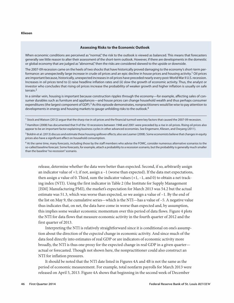
When economic conditions are perceived as “normal,” the risk to the outlook is viewed as balanced. This means that forecastersgenerally see little reason to alter their assessment of the short-term outlook. However, if there are developments in the domesticor global economy that are judged as “abnormal,” then the risks are considered skewed to the upside or downside.

The 2007-09 recession came on the heels of two shocks that have historically proved damaging to the economy’s short-term per-formance: an unexpectedly large increase in crude oil prices and an epic decline in house prices and housing activity.1 Oil pricesare important because, historically, unexpected increases in oil prices have preceded nearly every post-World War II U.S. recession.Increases in oil prices tend to (i) raise headline inflation rates and (ii) slow the growth of economic activity. Thus, the analyst orinvestor who concludes that rising oil prices increase the probability of weaker growth and higher inflation is usually on safeterrain.2

In a similar vein, housing is important because construction ripples through the economy—for example, affecting sales of con-sumer durables such as furniture and appliances—and house prices can change household wealth and thus perhaps consumerexpenditures (the largest component of GDP).3 As this episode demonstrates, nonpractitioners would be wise to pay attention todevelopments in energy and housing markets to gauge unfolding risks to the outlook.4

1 Stock and Watson (2012) argue that the sharp rise in oil prices and the financial turmoil were key factors that caused the 2007-09 recession.2 Hamilton (2008) has documented that 9 of the 10 recessions between 1948 and 2001 were preceded by a rise in oil prices. Rising oil prices alsoappear to be an important factor explaining business cycles in other advanced economies. See Engemann, Kliesen, and Owyang (2011). 3 Boldrin et al. (2013) discuss and estimate these housing spillover effects; also see Leamer (2008). Some economists believe that changes in equityprices also have a significant effect on household consumption.4 At the same time, many forecasts, including those by the staff members who advise the FOMC, consider numerous alternative scenarios to theso-called baseline forecast. Some forecasts, for example, attach a probability to a recession scenario, but the probability is generally much smallerthan the baseline “no recession” scenario.

2012, the data flows began to be better than expected, on net. All else equal, this was a signalthat in the fourth quarter the economy was strengthening by more than expected. However,when the advance estimate was released at the end of January 2013, real GDP for the fourthquarter of 2012 instead was shown to have declined at a 0.1 percent annual rate. This was farbelow the consensus forecast. Consistent with the NTI, though, subsequent revisions by theBEA slightly raised the advance estimate for real GDP growth in the fourth quarter from –0.1percent to 0.1 percent.

By contrast, Figure 4B shows that the NTI performed modestly better in the first quarterof 2013. Beginning in late February and early March 2013, the data began to come in consis-tently better than expected. In response, forecasters began raising their first-quarter estimatefor real GDP growth. When the advance estimate was released in late April 2013, the economywas shown to have grown at a 2.5 percent annual rate.

Although the NTI is a very simple metric for measuring momentum, there are a few draw-backs to consider. First, the NTI does not discriminate between the value added of expendi-tures (e.g., retail sales), employment, survey-based measures, or prices. A second criticism isthat the NTI assigns each series the same weight (equal importance). Thus, key data such aspayroll employment or housing starts should probably be assigned larger weights than seriessuch as wholesale inventories. One problem confronting all practitioners and nonpractitionersis the inevitability of data revisions. Although the NTI, by design, cannot account for subse-quent revisions, it does help minimize this problem because it includes survey data and othertypes of data that are not revised (e.g., consumer confidence or weekly initial claims). But ifthe goal is to use the latest data to get a reading on real GDP growth, then revisions are anissue that the nonpractitioner will need to confront.

Kliesen


–5

0

5

10

15

20

25

30

10/8/12 11/7/12 12/7/12 1/6/13 2/5/13 3/7/13

A. 2012:Q4

1/9/13 2/8/13 3/10/13 4/9/13 5/9/13–5

0

5

10

15

20

25

30

B. 2013:Q1

+1 = Better Than Expected –1 = Worse Than Expected +1 = Better Than Expected –1 = Worse Than Expected

Figure 4

Net Economic Tracking Index

SOURCE: Author’s calculations.

Principle #4: Beware of Data Revisions

As noted in the description of Principle 3, revisions to data compound the difficulty ofcorrectly identifying shocks and their significance in real time. These revisions occur largelybecause much of the source data collected by the U.S. government statistical agencies are basedon surveys of a sample of economic entities (firms, households, and government offices andagencies), rather than a survey of the universe of all economic entities. (This process is dis-cussed in the boxed insert above.) As an example of this process, consider the quarterly esti-mate for the growth of real GDP, which is subject to numerous revisions. These revisionsgenerally reflect updates in the underlying source data or new data based on more completesurveys or income tax records. Sometimes, revisions are made to prices or the underlyingstatistical methodology used by the government agencies to construct the estimate.

To see how revisions can dramatically change the portrait of the economy’s performance,consider the estimate of real GDP growth for the fourth quarter of 2007. According to theNBER, this quarter was the peak of the 2001-07 business expansion. As shown in Figure 5, theBEA released nine estimates of the annual rate of change for real GDP growth in the fourthquarter of 2007. In the advance estimate released in late January 2008, the BEA reported thatreal GDP rose at a 0.6 percent annual rate. However, when the annual National Income andProduct Accounts (NIPA) revision was released in late July 2008, the estimate for real GDPgrowth in the fourth quarter of 2007 was changed to –0.2 percent. This estimate was subse-quently changed to 2.9 percent per year in the 2010 annual NIPA revision but was subsequentlymarked back down by nearly 1.5 percentage points with the release of the July 2013 NIPArevision.

Kliesen


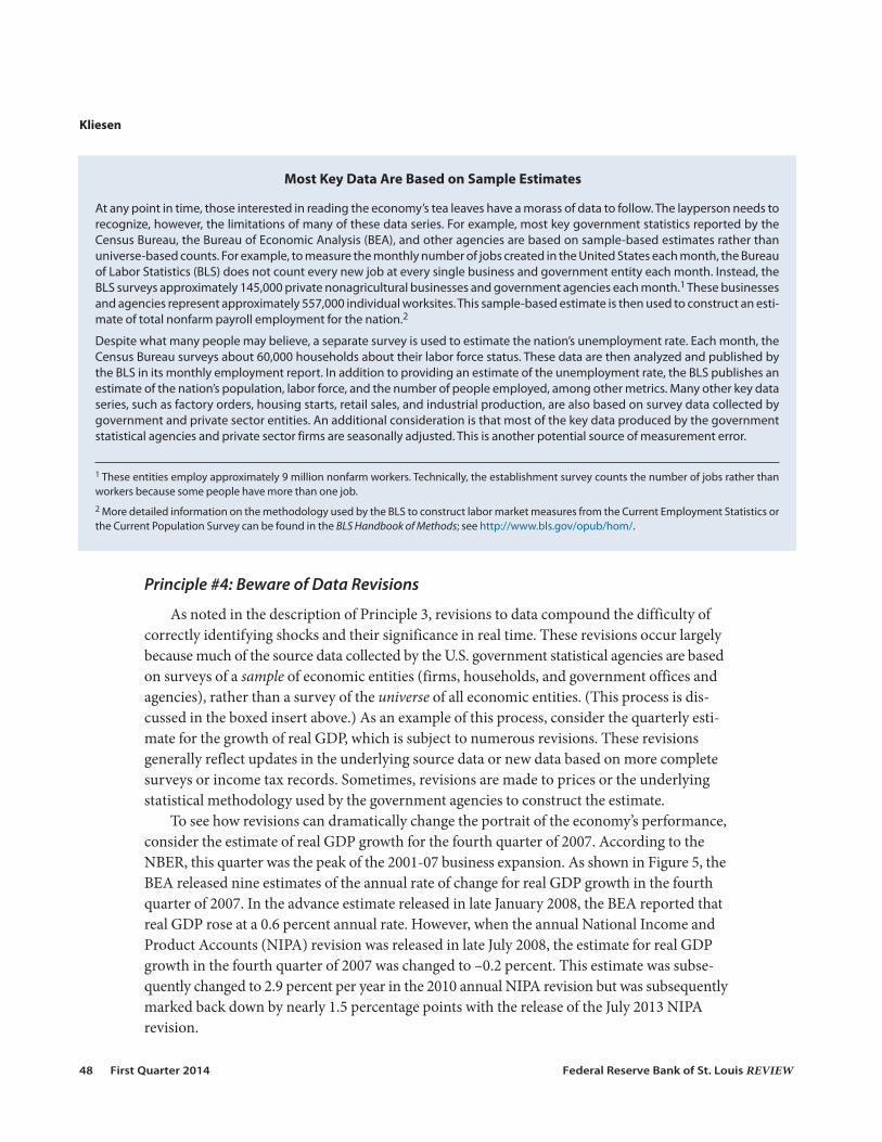
Most Key Data Are Based on Sample Estimates

At any point in time, those interested in reading the economy’s tea leaves have a morass of data to follow. The layperson needs torecognize, however, the limitations of many of these data series. For example, most key government statistics reported by theCensus Bureau, the Bureau of Economic Analysis (BEA), and other agencies are based on sample-based estimates rather thanuniverse-based counts. For example, to measure the monthly number of jobs created in the United States each month, the Bureauof Labor Statistics (BLS) does not count every new job at every single business and government entity each month. Instead, theBLS surveys approximately 145,000 private nonagricultural businesses and government agencies each month.1These businessesand agencies represent approximately 557,000 individual worksites. This sample-based estimate is then used to construct an esti-mate of total nonfarm payroll employment for the nation.2

Despite what many people may believe, a separate survey is used to estimate the nation’s unemployment rate. Each month, theCensus Bureau surveys about 60,000 households about their labor force status. These data are then analyzed and published bythe BLS in its monthly employment report. In addition to providing an estimate of the unemployment rate, the BLS publishes anestimate of the nation’s population, labor force, and the number of people employed, among other metrics. Many other key dataseries, such as factory orders, housing starts, retail sales, and industrial production, are also based on survey data collected bygovernment and private sector entities. An additional consideration is that most of the key data produced by the governmentstatistical agencies and private sector firms are seasonally adjusted. This is another potential source of measurement error.

1 These entities employ approximately 9 million nonfarm workers. Technically, the establishment survey counts the number of jobs rather thanworkers because some people have more than one job.2 More detailed information on the methodology used by the BLS to construct labor market measures from the Current Employment Statistics orthe Current Population Survey can be found in the BLS Handbook of Methods; see http://www.bls.gov/opub/hom/.

What should the nonpractitioner take away from this discussion? First, the data may notcorrectly portray the economy’s momentum. This possibility suggests that the nonpractitionershould take the monthly data flows and the consensus forecasts with a grain of salt. But whatis the alternative? After all, policymakers, FOMC members, businesspersons, and investorshave little choice but to react to the incoming data flows.13

One way a nonpractitioner can minimize the potential havoc caused by data revisions isto avoid point estimates. Thus, instead of becoming enamored with a forecast for real GDPgrowth of 3.5 percent (the point estimate), an interest rate of 3 percent, or an unemploymentrate of 6.5 percent, the nonpractitioner would attempt to assess whether the economic momen-tum revealed by forecast revisions and the NTI suggest something more likely on either sideof the point estimate. Another method of minimizing the impact of data revisions is to trackfinancial market conditions. Although there is the possibility of a chicken-versus-egg problemsince financial markets also react to incoming data flows that are subsequently revised, somefinancial market series have long been recognized for their leading indicator properties.

Principle #5: Track Financial Market Conditions14

Economic historians have long known that disturbances in the financial sector can havesignificant effects on the economy.15 Moreover, stabilizing the real economy through its inter-ventions in financial markets is one of the key reasons central banks exist.16 The FinancialPanic of 2008 provides another example of the financial sector’s far-reaching effects on themacroeconomy when asset prices and other key financial market indicators are changing sig-nificantly.17 Thus, for a more-complete portrait of the economy and potential changes in short-

Kliesen


0.6 0.6 0.6

–0.2

2.1

2.9

1.7 1.71.5

–0.5

0

0.5

1.0

1.5

2.0

2.5

3.0

3.5

Jan. 2008 Feb. 2008 Mar. 2008 Jul. 2008 Jul. 2009 Jul. 2010 Jul. 2011 Jul. 2012 Jul. 2013

Percent Change (Annual Rate)

Figure 5

Real-Time Estimates of Real GDP Growth During 2007:Q4

NOTE: Dates reflect the month in which the estimates were published.

SOURCE: Bureau of Economic Analysis and Haver Analytics.

term economic momentum, it is important for the nonpractitioner to understand and trackfinancial market conditions.

One of the key lessons policymakers learned from the 2007-08 experience is an old one:It is extraordinarily difficult to predict financial crises with any degree of confidence. But itcan also be difficult to monitor financial conditions because there are literally thousands ofdifferent types of financial indicators—ranging from stock price indexes, to interest rates ongovernment and corporate debt, to foreign exchange rates, to more elaborate indicators suchas credit default swaps and mortgage-backed securities.18 Fortunately, the nonpractitionercan overcome much of this difficulty by focusing on a handful of key indicators. Three cometo mind.

The first key financial indicator is a financial stress index (FSI). FSIs are designed tomeasure changes in financial conditions. For example, when financial market conditions areviewed as stable, then financial stresses tend to be relatively normal. In this situation, lendersare no more risk averse than normal and the volatility of asset prices, such as stock and bondprices, exhibits no unusual movements. By and large, financial market participants have arather sanguine view of the economy. By contrast, if lenders are becoming more risk averse,asset prices are falling, and volatility is increasing, then financial stresses are on the rise. Inthis instance, uncertainty about the health of the economy is increasing.

Rising levels of financial stress tend to weaken the real economy through a variety oftransmission mechanisms. These include reduced wealth, a reduction in bank lending, andbalance-sheet effects that reduce the value of a firm’s collateral. The key innovation of FSIs isthat they combine different types of financial market indicators into one index—much as theCPI is one measure of the economy’s price level constructed from tens of thousands of differ-ent prices on goods and services. For example, economic research has convincingly shownthere is significant information content, and thus predictive power, in the U.S. Treasury yield

Kliesen


September/October 2008

European Turmoil,May/June 2010

Week of August 5, 2011:S&P Downgrade and FOMC

–2

–1

0

1

2

3

4

5

6

12/31/93 12/31/97 12/31/01 12/31/05 12/31/09

Weekly Data

12/31/13

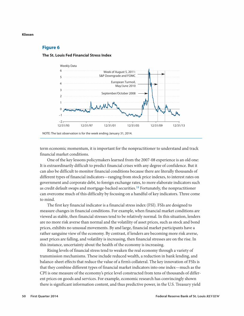
Figure 6

The St. Louis Fed Financial Stress Index

NOTE: The last observation is for the week ending January 31, 2014.

curve, commonly calculated as the difference between yields on 10-year Treasury securities and3-month Treasury bills. The yield curve tends to be upward sloping during times of positivegrowth in economic activity and tends to narrow as the pace of economic activity slows and—importantly—to invert before recessions.19

Another measure of financial market stress is the spread between 10-year Treasury securi-ties and Baa-rated corporate bonds. This interest rate spread, called the credit risk spread,accounts for default risks in private credit markets. Thus, if interest rates are rising and the paceof real GDP growth is slowing, firms tend to experience slowing sales, which adversely affectstheir revenues and thus their financial condition. In response, the risk associated with lendingto firms increases.

One well-known financial stress index that accounts for the information content in thesetwo interest rate spreads is the St. Louis Fed Financial Stress Index (STLFSI). Figure 6 plots theSTLFSI and shows that financial market stresses rose sharply prior to several recent economicupheavals that were transmitted to financial markets. These included recent developments inEurope, the downgrade of U.S. sovereign debt by Standard and Poor’s, and the unexpected down-ward revision in U.S. real GDP growth in July 2011 discussed previously. Empirical evidencesuggests that rising levels of financial stress are associated with weak or negative growth of indus-trial production and other measures of economic activity going forward.20

CONCLUSIONAnalyzing and forecasting the performance and direction of a large, complex economy like

that of the United States is exceptionally difficult. The process involves parsing a great deal ofdata, understanding key economic relationships, and assessing which events or factors mightcause monetary or fiscal policymakers to change policy. One purpose of this article is to reinforceseveral key principles that a nonpractitioner should use to analyze U.S. economic and financialmarket conditions. The nonpractitioner can do a reasonably good job of tracking changes in theeconomy’s momentum by taking advantage of freely available macroeconomic forecasts andtracking key data. �

Kliesen


NOTES1 Labor productivity is output per hour. Broadly speaking, output is the total value of real GDP. Real GDP measuresthe inflation-adjusted dollar value of goods and services produced by labor and property located in the UnitedStates; these are known as factors of production. A “real” series has been adjusted to remove the effects of changesin prices over time. This adjustment better accounts for increases in the production and consumption of goodsand services (i.e., volumes) in response to underlying factors that most affect supply and demand—such aschanges in population, productivity, and technological innovations. These real factors are the ones that lead toincreases (or decreases) in living standards, what economists term “economic growth.” See Gutierrez et al. (2007)for a primer on GDP and its construction.

2 In periods of economic recession, the level of real GDP is declining from one quarter to the next (at a negativegrowth rate).

3 A rough rule of thumb is that the NBER assumes that the inflection point occurred at the middle of the month.

4 The Blue Chip Consensus is a survey of roughly 50 private sector forecasters. For example, each forecaster submitshis or her forecast for real GDP growth and other key macroeconomic and financial variables for the current andupcoming year. The consensus is the simple average (mean) of these forecasts. These forecasts are published inthe Blue Chip Economic Indicators on or about the 10th of each month.

5 Economists use the Fisher equation to help analyze changes in interest rates. According to this equation, thenominal interest rate on, for example, a 30-year U.S. Treasury bond is the sum of (i) the real rate of interest earnedover this period and (ii) the average inflation rate expected over this period (the inflation premium, a premiumdemanded by lenders to compensate them for the expected inflation rate over the maturity of the bond). Thissimple formulation ignores other risk premiums embedded within these nominal interest rates and the complica-tion of selling a security before it matures, which can significantly affect the holding period rate of return on thebond.

6 Many sophisticated forecasting models, including those used by the staff economists at the Board of Governorsof the Federal Reserve, assume that the yield on, say, the 10-year Treasury security, is simply an average of a seriesof 1-year expected future interest rates. Thus, by changing the level of the overnight federal funds rate, the modelassumes that the Fed can affect the long-term interest rate.

7 Crude oil prices (measured by West Texas Intermediate) rose from a little more than $105 per barrel in March 2008to about $134 per barrel in July 2008 (monthly averages). Over the same period, the year-to-year percent changein the CPI increased from 4 percent to 5.6 percent.

8 The St. Louis Fed’s FRED (Federal Reserve Economic Data) database contains one of the world’s largest collectionsof freely available economic and financial data. FRED can be accessed at http://research.stlouisfed.org/fred2/.

9 From a GDP-accounting perspective, data that flow directly into real GDP—such as housing starts, retail sales,and factory shipments—help economists estimate whether the growth of real GDP is likely to change from itsprevious-quarter estimate. However, other data flows such as employment, initial unemployment claims, inflation,and consumer confidence might also be signals of changes in aggregate demand or supply and thus elicit reactionsfrom policymakers and financial market participants.

10 All these data, and more, are available on FRED, which currently contains more than 60,000 economic series.

11 Gavin and Kliesen (2002) provide a description and overview of the initial claims data. They also show that the ini-tial claims indicator has some statistically significant ability to predict monthly changes in payroll employment.

12 Many of these forecasts can be found on the “Calendar of Releases” (http://research.stlouisfed.org/publications/ usfd/cover.pdf ) published each week in the St. Louis Fed’s U.S.Financial Data publication (http://research.stlouisfed.org/publications/usfd/). Yahoo! provides an economic cal-endar with market forecasts of these and other variables (http://biz.yahoo.com/c/ec/201315.html).

13 Orphanides and Van Nordren (2002) have shown that the timeliness of the data and subsequent data revisionsmake it extremely difficult for monetary policymakers to identify the strength of real GDP relative to potential realGDP (the output gap) in real time.

14 This section draws from Kliesen, Owyang, and Vermann (2012).

15 See Kindleberger and Aliber (2005) or Reinhart and Rogoff (2009).

Kliesen


16 This principle is known as the lender of last resort. Walter Bagehot’s Lombard Street (1873) is a classic text on therole of central banks during financial crises.

17 Several other events around this period contributed to the rise of financial market instability. For example, see“The Financial Crisis: A Timeline of Events and Policy Actions” on the St. Louis Fed’s website (http://timeline.stlouisfed.org/).

18 Zheng (2012) provides a good summary of key financial indicators (such as the yield curve) for the noneconomist.

19 See Wheelock and Wohar (2009) for a summary of this research.

20 See Kliesen, Owyang, and Vermann (2012).

REFERENCESBagehot, Walter. Lombard Street: A Description of the Money Market. London: H.S. King, 1873.

Bernanke, Ben. “Transcript of Chairman Bernanke’s Press Conference.” June 19, 2013;http://www.federalreserve.gov/mediacenter/files/FOMCpresconf20130619.pdf.

Boldrin, Michele; Garriga, Carlos; Peralta-Alva, Adrian and Sánchez, Juan M. “Reconstructing the Great Recession.”Federal Reserve Bank of St. Louis Working Paper 2013-006B, February 2013, revised June 2013;http://research.stlouisfed.org/wp/2013/2013-006.pdf.

Engemann, Kristie M.; Kliesen, Kevin L. and Owyang, Michael T. “Do Oil Shocks Drive Business Cycles? Some U.S.and International Evidence.” Macroeconomic Dynamics, November 2011 (Suppl. S3), 15(3), pp. 498-517.

Gavin, William T. and Kliesen, Kevin L. “Unemployment Insurance Claims and Economic Activity.” Federal ReserveBank of St. Louis Review, May/June 2002, 84(3), pp. 15-28; http://research.stlouisfed.org/publications/review/02/05/15-28GavinKliesen.pdf.

Gutierrez, Carlos M.; Glassman, Cynthia A.; Landefeld, J. Steven and Marcuss, Rosemary D. “Measuring the Economy:A Primer on GDP and the National Income and Product Accounts.” Bureau of Economic Analysis, September 2007.

Hamilton, James D. “Oil and the Macroeconomy,” in Steven N. Durlauf and Lawrence E. Blume (eds.), The NewPalgrave Dictionary of Economics. Second Edition. New York: Palgrave Macmillan, 2008.

Kindleberger, Charles P. and Aliber, Robert. Manias, Panics, and Crashes: A History of Financial Crises. Fifth Edition.Hoboken, NJ: John Wiley & Sons, 2005.

Kliesen, Kevin L.; McCracken, Michael W. and Zheng, Linpeng. “Initial Claims and Employment Growth: Are We atthe Threshold?” Federal Reserve Bank of St. Louis Economic Synopses, 2011, No. 41, December 14, 2011;http://research.stlouisfed.org/publications/es/11/ES1141.pdf.

Kliesen, Kevin L.; Owyang, Michael T. and Vermann, E. Katarina. “Disentangling Diverse Measures: A Survey ofFinancial Stress Indexes.” Federal Reserve Bank of St. Louis Review, September/October 2012, 94(5), pp. 369-97;http://research.stlouisfed.org/publications/review/12/09/369-398Kliesen.pdf.

Leamer, Edward E. “Housing Is the Business Cycle,” in Housing, Housing Finance, and Monetary Policy. Proceedings ofthe 2008 Jackson Hole Economic Policy Symposium, Jackson Hole, Wyoming, August 30-September 1, 2007.Kansas City, MO: Federal Reserve Bank of Kansas City, 2008, pp. 149-233; http://www.kansascityfed.org/publicat/sympos/2007/PDF/Leamer_0415.pdf.

Orphanides, Athanasios and Van Norden, Simon. “The Unreliability of Output-Gap Estimates in Real Time.” Reviewof Economics and Statistics, November 2002, 84(4), pp. 569-83.

Poole, William. “Safeguarding Good Policy Practice.” Federal Reserve Bank of St. Louis Review, March/April 2005, 87(2, Part 2), pp. 303-06; http://research.stlouisfed.org/publications/review/05/03/part2/PanelDiscussion2.pdf.

Reinhart, Carmen N. and Rogoff, Kenneth S. This Time Is Different: Eight Centuries of Financial Folly. Princeton, NJ:Princeton University Press, 2009.

Stock, James H. and Watson, Mark W. “Disentangling the Channels of the 2007-2009 Recession.” Brookings Paperson Economic Activity, Spring 2012, pp. 81-135.

Kliesen


Wheelock, David C. and Wohar, Mark E. “Can the Term Spread Predict Output Growth and Recessions? A Survey ofthe Literature.” Federal Reserve Bank of St. Louis Review, September/October 2009, 91(5, Part 1), pp. 419-40;http://research.stlouisfed.org/publications/review/09/09/part1/Wheelock.pdf.

Zheng, Linpeng. “What Do Financial Market Indicators Tell Us?” Federal Reserve Bank of St. Louis Liber8 EconomicInformation Newsletter. January 2012; http://research.stlouisfed.org/pageone-economics/uploads/newsletter/2012/Lib0112.pdf.

Kliesen


Download - A Guide to Tracking the U.S. Economy models cannot predict. Second, most key data used to measure the economy and track its performance are often revised—and by substantial amounts

Top Related