
tlt\l1\1ERS1TV OF "
'4007.X'-,15
DESIGN OF FRONT-END AMPLIFIER FOR OPTICAL RECEIVER
IN 0.5 MICROMETER CMOS TECHNOLOGY
A THESIS SUBMITTED TO THE GRADUATE DIVISION OF THEUNIVERSITY OF HAWAI'I IN PARTIAL FULFILLMENT
OF THE REQUIREMENTS FOR THE DEGREE OF
MASTER OF SCIENCE
IN
ELECTRICAL ENGINEERING
AUGUST 2005
ByQianyi Yang
Thesis Committee:
Vinod Malhotra, ChairpersonAudra M. Bullock
Olga Boric-Lubecke

Acknowledgement
I would like to express my sincere gratitude to my advisor, Dr. Vinod Malhotra, for
his valuable suggestions, sound guidance and careful supervision throughout my master
program. I am also greatly indebted to Dr. Olga Boric-Luberke and Dr. Audra M. Bullock
for their support and advice in my experiment and research.
My gratitude is also devoted to all the people who help me in the past three years,
such as June Akers, Jason John and Myron Sugiki, who all contributed to my simulation
and experiment test. At last but not least, my gratitude is devoted to my family and all my
friends, whose love, patience and encouragement are the fundamental source of my
motivation and have supported me from the beginning to the end of this experiment,
especially to Tongxian Yang, Fan Jiang and Jincao Yu.
III

Abstract
The need for high speed optical receivers are being driven by high speed and wide
bandwidth optical communications demands. The front-end amplifier is a critical part in
optical receiver. Traditionally, it has been fabricated in expensive Gallium Arsenide and
silicon bipolar technologies. However, the quest for low cost, low power consumption
and small silicon area solutions in the commercial market has spurred a desire to
implement the circuit in Complementary Metal Oxide Semiconductor (CMOS)
technology.
This thesis describes the design of the front-end amplifier using AMI 0.5 CMOS
process. The target data rate is at least 500Mb/s suitable for local area network
application. The front-end amplifier is divided into two stages, the transimpedance
amplifier (TIA) and the limiter amplifier (LA). The resistive feedback TIA topology is
selected for the TIA design. The LA circuit is realized by cascading two resistive load
differential amplifiers with one buffer.
The simulation results show that the designed TIA achieves 374.4MHz bandwidth
with a corresponding achievable data rate of - 535Mb/s. Its transimpedance gain is 4 kQ
The LA bandwidth is 586.8MHz and the output swing is 4.2V.
The fabricated TIA and the front-end amplifier are experimentally tested to validate
performance in the frequency range up to 24MHz. The simulation and the experimental
results exhibit good agreement at these frequencies.
IV

LIST OF TABLES
Table Page
1.1 Front-end Amplifier Fabricated in Different Technology .4
2.1 Characteristics of inductive peaking 19
2.2 Recent reported CMOS TIA circuits 19
2.3 The ratio of 0)_3dB over 0)0 as of N 21
2.4 Recent reported CMOS LA circuits 24
3.1 Proposed Front-end Amplifier Specifications 28
3.2 TIA circuit parameters 29
3.3 The parameters of LA circuit 33
4.1 Simulated DC operation points of the resistive feedback TIA .38
4.2 Input and output resistance ofTIA , 38
4.3 Simulated and tested DC operation points of resistive feedback TIA .47
4.4 DC operation points of LA 52
4.5 Input and Output Resistance of LA ~ 52
4.6 Simulated Front-end Amplifier Operation Point. 59
4.7 Input and out resistance of front-end amplifier 59
4.8 Simulated and tested DC operation points of front-end amplifier 63
4.9 The summary values 70
v

Figure
Figure 1.1
Figure 1.2
Figure 2.1
Figure 2.2
Figure 2.3
Figure 2.4
Figure 2.5
Figure 2.6
Figure 2.7
Figure 2.8
Figure 2.9
Figure 2.10
Figure 2.11
Figure 3.1
Figure 3.2
Figure 3.3
Figure 3.4
Figure 3.5
Figure 3.6
LIST OF FIGURES
Page
Fiber optical system 1
Front-end amplifier composed of TIA and LA stages 2
A TIA circuit and its equivalent circuit 8
Common-gate TIA 10
Resistive feedback TIA 12
Implementation of resistive feedback TIA 13
TIA with Capacitive feedback 14
Resistive feedback TIA with series inductive peaking 17
The common-source TIA with shunt inductive peaking 18
Cascade of small-signal amplifiers 21
Resistive Load Differential Amplifier Schematic 22
Small-signal model of differential half-circuit 23
LA configuration 23
The Circuit Design Flow 26
Front-end Amplifier Block Diagram 27
Resistive Feedback TIA schematic 29
AC Half-circuit of TIA 30
Series Inductive Peaking 32
Shunt Inductive Peaking 32
VI

Figure 3.7
Figure 3.8
Figure 3.9
Figure 3.10
Figure 3.11
Figure 4.1
Figure 4.2
Figure 4.3
Figure 4.4
Figure 4.5
Figure 4.6
Figure 4.7
Figure 4.8
Figure 4.9
Figure 4.10
Figure 4.11
Figure 4.12
Figure 4.13
Figure 4.14
Figure 4.15
Figure 4.16
LA circuit 34
Front-end Amplifier 35
Whole Circuits Layout 36
Front-end Amplifier Layout.. 37
TIA Circuit Layout 37
Simulation schematic of the TIA 39
Differential sinusoid inputs of the TIA at IOMHz 40
Differential sinusoid outputs of the TIA at IOMHz 40
Output amplitude vs. frequency 40
The bandwidth of TIA vs. input diode capactiance 41
Differential inputs of square wave at 1KHz 42
Output response of the TIA at 1KHz 42
Output response of the TIA at 10KHz 43
Output response of the TIA at 100MHz 43
Output response of the TIA at 400MHz 44
Resistive feedback TIA test setup 45
Differential signals generated by the pulse wave generator 46
Outputs of the TIA at 1KHz 48
Outputs of the TIA at 10KHz 48
The layout of PCB testboard 49
The schematic of PCB testboard 49
Vll

Figure 4.17
Figure 4.18
Figure 4.19
Figure 4.20
Figure 4.21
Figure 4.22
Figure 4.23
Figure 4.24
Figure 4.25
Figure 4.26
Figure 4.27
Figure 4.28
Figure 4.29
Figure 4.30
Figure 4.31
Figure 4.32
Figure 4.33
Figure 4.34
Figure 4.35
Figure 4.36
Figure 4.37
The output amplitude of TIA vs. frequency 50
Outputs of TIA at 1OMHz 51
One output of TIA at 50MHz 51
The simulation schematic of the LA circuit.. 53
The input voltage swing vs. output voltage swing of LA 54
Voltage gain vs. Bandwidth 55
The square wave inputs of LA at 1MHz 56
The square wave outputs of LA at 1MHz 56
The inputs of triangle waveform of the LA at IMHz 57
The outputs of LA at IMHz 57
Simulation schematic of the front-end amplifier 58
Output response of front-end amplifier at 1KHz 60
Output response of front-end amplifier at 10KHz 60
Output response of front-end amplifier at 100MHz 61
Output response of front-end amplifier at 500MHz 61
Front-end amplifier test setup 62
Output of front-end amplifier at 1KHz frequency 63
Output of the front-end amplifier at 10KHz frequency 64
Output swing of front-end amplifier vs. frequency 65
Outputs of front-end amplifier at 100KHz 65
Outputs of front-end amplifier at 1MHz 66
Vlll

Figure 4.38
Figure 4.39
Figure 4.40
Figure 4.41
Simulation schematic for series inductive peaking 67
Bandwidth enhancement vs. inductance by series inductive peaking 67
Simulation schematic of shunt inductive peaking 68
Bandwidth enhancement vs. inductance by shunt inductive peaking 69
IX

TABLE OF CONTENTS
ACKNOWLEDGEMENT III
ABSTRACT IV
LIST OF TABLES V
LIST OF FIGURES VI
CHAPTER 1. INTRODUCTION 1
CHAPTER 2. LITERATURE REVIEW 6
2.1
2.1.1
2.1.2
2.1.3
2.2
2.2.1
2.2.2
2.2.3
2.2.4
2.2.5
2.3
2.4
2.4.1
2.4.2
2.4.3
TIA PERFORMANCE PARAMETERS 6
Bandwidth 6
Transimpedance Gain 7
Input-referred Noise 7
TIA DESIGN TOPOLOGIES 9
Common-gate TIA 9
Resistive Feedback TIA 11
Capacitive Feedback TIA 14
Inductive Peaking 16
Recently Reported TIA circuits 19
LA PERFORMANCE PARAMETERS 19
LA DESIGN TOPOLOGIES 20
Cascaded Gain Stages 20
Resistive Load Differential Amplifier 22
Recently Reported LA circuits 24
CHAPTER 3. THESIS PROJECT CIRCUIT DESIGN 25
3.1 DESIGN TOOLS AND DESIGN FLOW 25
x
3.2 DEFINITIONS OF SPECIFICATIONS 27
3.3 TIACIRCUITDESIGN 28
3.3.1 Schematic and Parameters 28
3.3.2 Circuit Implementation 30
3.3.3 Inductive Peaking 31
3.4 LA CIRCUIT DESIGN 33
3.5 FRONT-END AMPLIFIER CIRCUIT 35
3.6 LAYOUT IMPLEMENTATION 36
CHAPTER 4. SIMULATION AND EXPERIMENT RESULTS 38
4.1 RESISTIVE FEEDBACK TIA 38
4.2 LIMITER AMPLIFIER 52
4.3 FRONT-END AMPLIFIER 58
4.4 INDUCTIVE PEAKING 66
4.5 SUMMARy 69
CHAPTER 5. SUMMARY AND CONCLUSION 71
REFERENCES 73
xi

Chapter 1. Introduction
Fiber optical communication system plays an important role in present communication
industry. It offers several advantages including low cost, small size, low transmission loss
and high bandwidth compared to conventional electrical communication based on Copper.
It is widely used in high-speed, wide-bandwidth applications such as local area networks
(LANs) and fiber to home (FfTH) [1,2]. Its architecture is illustrated in Figure 1.1.
Laser Diode
-z.. (.....)'-- ~)-z..
Laser Driver
Photo-diode
Front-end Amplifier
Transmitter
Figure 1.1
Fiber
Fiber optical system
Receiver
It consists of a transmitter, a fiber and a receiver. The modulation of the electrical
signal to light takes place at the level of the transmitter. Relatively low-speed parallel
electrical signals are transformed to high-speed serial signal by a multiplexer (MUX).
Subsequently, the electrical signal is fed to the laser driver and light is produced by the
laser diode according to the input current. After this transmitter stage, the light is carried
1

to a remote destination by the fiber. The conversion of the incoming light back to
electrical signals takes place at the side of the receiver. There, a photodiode converts the
incoming light to current. Next, a front-end amplifier converts the current back to an
electrical signal. Finally, a demultiplexer (DMUX) transfers the series data back to
parallel data [3].
The project addressed In this thesis is the design of a front-end amplifier. The
amplifier consists of two stages, as shown in Figure 1.2. The first stage is a
transimpedance amplifier (TIA), and the second stage is a limiting amplifier (LA).
Front-end Amplifier
I
I
Cdiode IIII
Figure 1.2 Front-end amplifier composed of TIA and LA stages
The TIA is the most critical part of an optical receiver design because its noise, gain
and frequency performance largely determines the overall data rate that can be achieved
in an optical system. The function of a TIA is to convert the input current from the
2

external photodiode to a voltage output. The TIA has a large transimpedance gain and a
low sensitivity to the photodiode capacitance. These characteristics are important because
the input photocurrent is very small, typically varying from about 1O~A to 20~A. In
addition, the photodiode capacitance is usually large, ranging from about O.3pF to 1pF
[4,5,6,7].
Although the structure of TIA offers large gain, the signal produced by TIA still
suffers from small amplitude, usually on the order of a few tens of millivolts. Therefore,
the TIA must be followed by a LA, which boosts the voltage swing and matches the
output impedance to drive the DMUX [2].
There are several competing technologies such as Silicon Bipolar (Si-bipolar),
Gallium Arsenide (GaAs), Silicon Germanium (SiGe), Silicon-On-Insulator (SOl) and
Complementary Metal Oxide Semiconductor (CMOS) to design front-end amplifiers.
Table 1.1 lists several front-end amplifiers which are reported in the literature
[1,7,8,9,10,11]. The technologies of Si-bipolar, GaAs, SiGe and SOl offer large
bandwidth transistors. Therefore it is easier to design high speed front-end amplifier
using these processes than to design it using CMOS technology. However, the needs for
low cost, low power consumption and small silicon area have motivated front-end
amplifier to be implemented in CMOS. CMOS technology offers System-On-Chip (SOC)
solution because it can integrate the analog and digital components on a same chip. In
addition, the performance of CMOS technologies is being improved constantly and
consistently. In fact, submicrometer CMOS technologies now exhibit sufficient
performance for radio-frequency applications in the 1-2GHz range and higher.
3

Process Feature Size Data Rate
Si-bipolar 0.3 11m 5Gb/s
GaAs 0.5 11m 1.7Gb/s
SiGe 0.5 11m 2Gb/s
SOl 0.5 11m 700Mb/s
CMOS 0.6 11m 250Mb/s
CMOS 0.35 11m 2.5Gb/s
Table 1.1 Front-end Amplifier Fabricated in Different Technology
The objective of this thesis project is to design a front-end amplifier in CMOS
technology. The data rate is aimed to be larger than 500Mb/s so that it is comparable
with current LAN data rates and sufficiently fast to support real-time video applications.
The circuits are fabricated in AMI 0.5 J!ffi C5N (AMI05), which is a 5-Volt, N-Well
process. It has three metal layers, two poly layers, and a high resistance layer. Stacked
contacts are supported. In this process, the minimum allowable drawn length is
0.6 J!ffi while its effective gate length is 0.5 11m.
This thesis consists of five chapters. Chapter 2 illustrates and compares several
possible topologies for TIA. It also examines the design issues of LA. Chapter 3
describes the implementation of TIA and LA circuits using AMI 0.5 11m CMOS
technology. Additionally, it shows the layout of the front-end amplifier system. Chapter
4

4 illustrates the simulation results and experiment tests. Chapter 5 is the conclusion of the
thesis with suggestions for future design considerations.
5

Chapter 2. Literature Review
Many papers in literature present the different topologies of the TIA and LA circuit
design using CMOS process. This chapter summarizes several design topologies which
are widely used. The concerns and motivations involved in the TIA and the LA circuit
design are also presented.
2.1 TIA Performance Parameters
As previously mentioned, the TIA is the most critical part of an optical receiver. The
main design challenges are trade-offs between transimpedance gain, bandwidth and input
noise current. Before examining the TIA design topologies, a brief description of these
parameters is presented below.
2.1.1 Bandwidth
The bandwidth of a TIA determines the data rate of an optical receiver. For a non
return to zero (NRZ) data format, the bandwidth should be set to 0.7 times the data rate
[1,12]. This result is due to the compromise between the intersymbol interference (lSI)
and noise. In order to achieve better performance for NRZ data, the bandwidth should be
maximized to reduce the lSI. On the contrary, the bandwidth cannot be too large because
while a TIA amplifies the signal, it also amplifies the noise at different frequency as well.
According to this rule, because the desired data rate of this thesis project is 500Mb/s, the
bandwidth of the TIA should set to be larger than 350MHz.
(3dB =DataratexO.7 =500xO.7 =350MHz (2.1)
6

2.1.2 Transimpedance Gain
The transimpedance gain is the ratio of the output voltage amplitude over the input
current amplitude at low frequency. It is given by
(2.2)
The gain of the TIA is expected to be as large as possible to enhance the sensitivity of the
system. However, the gain is limited by the supply voltage headroom. Additionally, the
gain cannot be too large in order to achieve large bandwidth. For example, the gain of the
TIA may only be 530 Q in order to achieve high bandwidth of 1.75GHz with supply
voltage of 3V [1].
2.1.3 Input-referred Noise
The parameter of the input-referred noise is used to compare the noise generated by
different TIA circuits. It is a fictitious quantity which cannot be observed in a circuit.
This parameter does not depend on the gain of the TIA. As defined in [3], "input-referred
noise is the value that, if applied to the input of the equivalent noiseless circuit, produces
an output noise equal to that of the original, noisy circuit."
To illustrate how to calculate the input-referred noise, a TIA and its equivalent circuit
is shown in Figure 2.1. The transimpedance gain is equal to RL • We assume that the
thermal noise of RL is the only source of noise. The noise per unit bandwidth is given by
(2.3)
where k is the Boltzmann's constant and T is the temperature of the circuit.
7

The output integrated noise is given by
2
V2=f=4kT R II 1 df= kTn,on! 0 R Leo2 f C
L oj 1t 0
(2.4)
Because the TIA has a transimipedance gain of R L ' its total input-referred noise current
is equal to
r -V;'on! _ kTn,in-~-R2C
L L 0
(2.5)
Figure 2.1 A TIA circuit and its equivalent circuit
The input-referred noise generated from the TIA directly determines the signal to
noise ratio (SNR) of the optical network as indicated in the following equation
SNR= linIn,in
8
(2.6)

where lin is the input current and In,in is the input-referred noise. Because large SNR is
desired in optical network, the TIA circuit which offers small input-referred noise is
usually preferred.
2.2 TIA Design Topologies
There are many topologies of the TIA developed in order to achieve large
transimpedance gain, large bandwidth and small input-referred noise. Three topologies
are widely used, including the common-gate TIA, the resistive feedback TIA and the
capacitive feedback TIA. These topologies are presented and their input-referred noises
are compared. The inductive peaking topology is discussed later as an effective method
of bandwidth enhancement.
2.2.1 Common-gate TIA
The common-gate (CG) amplifier stage is widely used in the open loop TIA topology
since it exhibits low input impedance. The circuit is illustrated in Figure 2.2. The Ml
transistor offers the common-gate gain. The M2 transistor supplies bias current for the
Ml transistor. In order to simplify the AC signal analysis, only the diode capacitance is
taken into account because it is quite larger than other parasitic capacitance values. In
addition, the body effect of the transistor Ml is neglected. Under these assumptions, the
transfer function is given by
VOUl = gmlROlin gml+COS
(2.7)
Substituting s=O in Eq (2.7), we find that the DC transimpedance gain can be written as
9

The bandwidth is given by
f =~-3dB 2nC
o
where the gml is the transconductance of the Ml transistor.
(2.8)
(2.9)
I-m
Figure 2.2
f-----o Vout1
I •Vbl
~Vb2
M2
Common-gate TIA
The common-gate TIA is able to provide a large transimpedance gam and broad
bandwidth. However, its input-referred noise is relatively large because the noise currents
due to the transistor M 2 and the resistor R o are directly referred to the input. It is given
by
2 2 -2- 4kTInin=InR + InM =--+4kTygm2
, , D , 2 Ro
where y is the threshold voltage parameter of the M2 transistor.
10
(2.10)

The design of the common-gate TIA has several constraints. According to Eq (2.9), in
order to increase the bandwidth, the quantity of gml must be maximized. In other words,
the width or the bias current of the Ml transistor should be increased. In the first situation,
if the width is increased, the parasitic capacitance of the Ml transistor will also increase
such that it will eventually limit the bandwidth. In the second situation, if the bias current
is increased, the voltage drop across R o must increase, requiring a greater supply voltage.
In addition, if M2 transistor is made wider, it brings more noise to the TIA because it
makes the second term ofEq (2.10) larger [5].
2.2.2 Resistive Feedback TIA
The topology of the resistive feedback TIA is demonstrated in Figure 2.3. It uses a
resistor to sense the voltage at the output and returns a proportional current to the input.
The transfer function is given by
(2.11)
The transimpedance gain is given by
(2.12)
The bandwidth is given by
(2.13)
11

Rp
Vout
Figure 2.3
The input noise current is given by
Resistive feedback TIA
12 . = 4kT + V;'An,m R R 2
p P
(2.14)
The first term is the noise of R p which is directly referred to the input. The second term
is the noise from the amplifier stage.
Eq (2.10) and Eq (2.14) reveal the critical difference between the input-referred noise
between the CO TIA and the resistive feedback TIA. Although the first term in both
equations plays the same role indicating the resistor thermal noise, the second term is not
the same. In the resistive feedback TIA, if the R p is large enough, the second term in
Eq (2.14) may be quite smaller than the second term in Eq (2.10). It is a practical
approach because the R p resistor does not carry any bias current and its value does not
limit the supply voltage headroom. Therefore, the resistive feedback TIA is able to offer
smaller noise than the CO TIA.
12

The implementation of the resistive feedback TIA is illustrated in Figure 2.4. The M1
transistor acts as the amplifier stage, and M2 supplies bias current for the M1 transistor.
The open-loop gain is given by
(2.15)
voo
RoRp
Voul
Figure 2.4 Implementation of resistive feedback TIA
The circuit suffers from one drawback. The bandwidth is limited because the value of
Ro is limited by supply voltage. The voltage drop across Ro cannot exceed
VOO-VGS2-VGSI' Therefore, the Ro resistance has to be relatively small. The open-loop
gain cannot be very large. According to Eq (2.13), the bandwidth is also limited [13, 14].
13

2.2.3 Capacitive Feedback TIA
Figure 2.5 illustrates the capactive feedback TIA, where C1 senses the voltage across
Cz and returns a proportional current to the input. If the open-loop gain of the amplifier
stage satisfies A» 1, then the ratio of the output current to the input current is given by
VDD
(2.16)
Figure 2.5 TIA with Capacitive feedback
It suggests that the circuit can operate as a current amplifier. With a resistor R D tied to
the drain of the M[ transistor, it provides a transimpedance of
CR =(I+-Z )R
T C D[
14
(2.17)

The bandwidth of the circuit is given by
(2.18)
The input-referred noise is given by
(2.19)
The first term is the noise of RD which is directly referred to the input. The second term
is the noise from the amplifier stage.
For fair comparison of the input-referred noises generated by the capacitive feedback
TIA and the resistive feedback TIA, it is assumed that both circuits have the same gain.
In other words, we have
(2.20)
By substituting the Eq (2.20) to Eq (2.14), the input-referred noise of the resistive
feedback TIA is given by
v2 ( 1 )24kT n,A R
12 Dn,in =--+ C
RD 0+_2 )2
Ct
(2.21)
At low frequency, when IC2sl<_1_, the capacitive feedback TIA generates smaller noiseRD
than the resistive feedback TIA. However, when the frequency increases so that
IC2sl>_1_, the resistive feedback TIA offers smaller noise [15]. Although this topology isR D
15

able to supply high transimpedance gain, it is able to achieve low noise only at low
frequency.
In summary, among the three topologies as discussed above, the resistive feedback
TIA offers the smallest noise at high frequency. Therefore, it is selected for the TIA
circuit design in the thesis project.
2.2.4 Inductive Peaking
The limitation of the bandwidth of TIA is primarily due to the large capacitance either
at the input or the output nodes. Therefore, if an inductor is inserted to resonate with the
capacitance, the bandwidth can be enhanced. This method is called "inductive peaking",
and may be applied to the three topologies discussed above. There are two types of
inductive peaking, series peaking and shunt peaking.
Series Inductive Peaking
Series inductive peaking utilizes the inductor series with the input of the TIA. An
example of the resistive feedback TIA with series inductive peaking is shown in Figure
2.6. The transfer function is given by [3]
(2.22)
where ~= R F# and co~=_I_. If we set ~=J212 then the bandwidth of the TIA is2(A+l)L CoL
given by
16

f = J2A-3dB 2nR FeD
(2.23)
Hence, the bandwidth is increased by approximately 41 % with an overshoot of 4.3%.
RF
You!
Figure 2.6 Resistive feedback TIA with series inductive peaking
However, series inductive peaking suffers from the requirement of using very large
inductor, usually on the order of luH. The monolithic inductor cannot offer this large
value. Therefore, it is possible to use a bond wire instead, which means that the length
and shape of the wire and the capacitance of the photodiode must be controlled tightly.
Shunt Inductive Peaking
Shunt inductive peaking occurs when the inductor appears in parallel with the output.
An example of common-source TIA with shunt inductive peaking is illustrated in
Figure 2.7. In order to simplify the analysis, only the output capacitance is taken into
account.
17

VDD
Voul
VOUl
Figure 2.7 The common-source TIA with shunt inductive peaking
The transfer function is given by [3]
(2.24)
The bandwidth is
(2.25)
Table 2.1 demonstrates the bandwidth enhancement ratios and overshoot values
according to different values of S. With the margin requirement for process and
temperature variation, an overshoot of 7.5% offers a reasonable compromise between the
control over the step response and the improvement in bandwidth. Therefore, according
to Table 2.1, the bandwidth can be enhanced by 82% [16].
18

~ 0.69 0.64 0.59
Bandwidth enhancement 78% 82% 84%
Overshoot 5% 7.5% 10%
Table 2.1 Characteristics of inductive peaking
2.2.5 Recently Reported TIA circuits
Table 2.2 summarizes several recent reported CMOS TIA circuits using the topologies
discussed above.
Technology Supply Topology Bandwidth Gain
Design in [5] 0.8~m 5V Common-Gate 950MHz 100Q
Design in [4] 0.7~m 5V Resistive Feedback 1.5GHz 1kQ
Design in [15] 0.6~m 3V Capacitive Feedback 550MHz 6.7kQ
Design in [16] 0.6~m 5V Shunt Inductive l.2GHz 1.6kQ
Peaking
Table 2.2 Recent reported CMOS TIA circuits
2.3 LA Performance Parameters
The bandwidth and the output swing are two critical parameters for the LA circuit
design. Unlike the TIA, whose bandwidth should set to be approximately 70% of the data
rate, the bandwidth of the LA is designed to be equal to the data rate. This is because if
19

two stages with equal bandwidths are cascaded, then the overall small-signal bandwidth
is narrower.
The output swing of the LA must be large enough to drive the following DMUX stage.
It must be at least 250mV. In some optical receiver circuits, it may be as large as full rail-
to-rail swing [3,4, 12].
2.4 LA Design Topologies
The cascaded gain stages are used to implement the role of a limiter amplifier. In
order to understand the properties of LA, the performance of the cascaded gain stages is
studied. Later, the circuit of the gain stage is demonstrated.
2.4.1 Cascaded Gain Stages
As illustrated in Figure 2.8, two gain stages are cascaded. Assuming they have the
same voltage gain Ao ' output resistance Rout and load capacitance CL , the overall
transfer function is given by [3]
2
H(s)= (2.26)
1where 0)0= is the -3dB bandwidth of each stage. Therefore, the bandwidth is
RoutCL
given by
(2.27)
20

From Eq (2.27), we know that cascading two identical stages decreases the bandwidth by
about 36%. Similarly, for N identical stages, the -3dB bandwidth is given by
ffi -3dB =ffio~~-1 (2.28)
Figure 2.8 Cascade of small-signal amplifiers
Table 2.3 illustrates the ratio of the overall bandwidth over the single stage bandwidth
as a function of N. Typically limiter amplifier employs no more than five gain stages due
to the rapid decrease of overall bandwidth as increasing the number of gain stages.
N 2 3 4 5
ffi -3dB0.63 0.53 0.45 0.4
ffio
Table 2.3 The ratio offfi_3dB over ffioas ofN
21

In order to know the output swing of the LA, we need to examine the total gain of the
LA. It is given by
(2.29)
This result from small-signal analysis only offers a conservative estimation for the output
swing of the LA. Typically, the second or third gain stage of the LA senses sufficiently
large input swing so that it operates in the switching'state. Therefore, it is able to offer
large output swing.
2.4.2 Resistive Load Differential Amplifier
The simplest circuit for the gain stage is resistive load different amplifier. The circuit
is shown in Figure 2.9. Due to the symmetry of the design, the small signal performance
can be analyzed with the aid of half-circuit model as illustrated in Figure 2.10.
V DD- -- -
voutl voutl
Vinl~ ~Vinl
Figure 2.9 Resistive Load Differential Amplifier Schematic
22

o+
R c+
Vd-out2.
Figure 2.10
The gain expression is [12]
The bandwidth is
Small-signal model of differential half-circuit
f =_1_-3dB 2nRC
(2.36)
(2.37)
By cascading several resistive load differential amplifiers, a LA is shown as Figure
2.11. As can be seen, because the last stage is operated in non-linear region, the small
signal can be converted into large output swing signal exhibiting short rise and fall time.
.,...........-----,.......,---......,-.... VDD
Figure 2.11 LA configuration
23

2.4.3 Recently Reported LA circuits
Several recent reported CMOS LA circuits using the topology discussed above are
summarized in Table 2.4.
Technology Supply Bandwidth Output Swing
Design in [12] O.18~m 3.3V 1.10Hz 300mV
Design in [7] O.5~m 3.3V 10Hz 3.1V
Design in [17] O.35~m 5V 1.40Hz 280mV
Table 2.4 Recently reported CMOS LA circuits
24

Chapter 3. Thesis Project Circuit Design
This Chapter illustrates the implementation details of the front-end amplifier using the
AMI05 process. First the design tools and the circuit design flow are introduced.
Followed by that is the detailed design issues on the TIA and the LA circuits. Finally, the
circuit layout is presented.
3.1 Design Tools and Design Flow
The circuit design is done using the Cadence Design Environment (CDE) and NCSU
design kit. CDE is an Electronic Design Automation (EDA) environment, which
integrates different tools for integrated circuit (IC) design together in a single framework.
Therefore, it is able to support all the stages of an IC design.
NSCU Design Kit is supplied by North Carolina State University. It is a set of
configuration and technology-related files to customize the design environment for the
AMI05 process. The files includes layer definitions, parasitic capacitance, layout cells,
simulation parameters, the rules for Design Rule Check (DRC) and the rules for Layout
versus Schematic (LVS) verification.
The flow chart for the circuit design is shown in Figure 3.1. First, the specifications
for the circuit such as the bandwidth are determined. Next, the parameters of the circuit
such as the resistor value are set according to the results of hand calculation.
Subsequently, a schematic view of the circuit is created using the Cadence Composer
followed by the circuit simulation using Spectre. After the circuit specifications are
satisfactorily met, the circuit layout is created using the Virtuoso Layout Editor.
25

LayoutVerifiaction
c::===:::::::::::::=- Cadence Composer
c======:::::::::=- Spectre
c::===:::::::::::::=- Virtuoso Layout Editor
c=====:::::::::::::::=- DRC, LVS
NO
Post-LayoutSimulation
c=====::::::::::====- Spectre
Figure 3.1 The Circuit Design Flow
26

The DRC verifies whether the layout satisfies the geometric constrains of the AMI05
process. The LVS compares the layout to the schematic to ensure that the intended
functionality is implemented. If the layout passes the DRC and LVS check, post-
simulation is carried by plugging the parasitic capacitors of the layout into the original
schematic. After the results of the post-simulation meet the circuit specification, the
layout is converted to CIF format and sent to be fabricated.
3.2 Definitions of Specifications
Figure 3.2 illustrates the block diagram of the front-end amplifier designed in the
project. As previously mentioned, the data rate of the front-end amplifier should be larger
than 500Mb/s. For TIA, the bandwidth should be larger than 350MHz. For LA, the
bandwidth should be larger than 450MHz.
A photodiode is expected to produce a 20 IlAp_p current signal. The TIA should
amplify the current signal to be larger than 60 mVp_p' Therefore, the transimpedance gain
of TlA should be larger than 3 kQ. The LA should be able to boost the swing to 3.5V at
least in order to drive the DMUX.
Throughout the following documentation, the circuit design will be verified with the
specifications listed in Table 3.1.
r - - iro~t--;nd ~PIifi-;r-', ,, ,
20IlAw, ,, TIA >'-,-~ DMUX
1 II 1L I
Figure 3.2 Front-end Amplifier Block Diagram
27

Parameter Value
Minimum Data Rate 500Mb/s
TIA Minimum Bandwidth 350MHz
TIA Minimum Gain 3k.Q
LA Minimum Bandwidth 450MHz
LA Minimun Output Swing 3.5V
Diode Light Current, iD 20llA
Diode Capacitance, CD O.5pF
Table 3.1
3.3 TIA Circuit Design
Proposed Front-end Amplifier Specifications
As mentioned in the previous chapter, the TIA circuit is designed using the resistive
feedback topology. This topology is chosen because it generates the smallest noise while
it offers high impedance gain and acceptable bandwidth. Additionally, it does not need to
use any capacitor or inductor, which the AMI05 process can not supply.
Although the inductive peaking topology cannot be implemented due to the limitation
of the AMI05 process, it is still studied in the simulation level because it is an effective
way to enhance the bandwidth.
3.3.1 Schematic and Parameters
The TIA schematic is shown in Figure 3.3. The TIA circuit is based on the circuit as
illustrated in Figure 2.4. However, it is modified to differential circuit in order to
28

suppress the fluctuations of power supply and substrate noise. The RI resistor and MI,
M2 transistors forms a current mirror to supply a constant current flow for the differential
circuits. The transistors of M3, M4, M5 and M6 are differential pairs of resistive
feedback TIA. The M3 and M5 transistors act as common-source amplifier to provide the
voltage gain. The R f resistors offer resistive feedback. The diode-connected PMOS
transistors, M4 and M6, are used as load resistors. All the transistors have a gate length of
0.6/lm. The rest of the circuit parameters are listed as Table 3.2.
Vdd
M6
out! out2
RlRf
M5 in2
MI M2
gnd
Figure 3.3 Resistive Feedback TIA schematic
MI M2 M3 M4 M5 M6 RI Rf
9/lm 9/lm 138/lm 3/lm 138/lm 3/lm 1O.6IkQ 4.53kQ
Table 3.2 TIA circuit parameters
29

3.3.2 Circuit Implementation
The AC half-circuit of the differential TIA is shown in Figure 3.4. M4 can be viewed
as a resistor load. The value of the resistor is
where the gm4 is the transconductance of M4 PMOS.
The voltage gain of the common source amplifier is given by
(3.1)
A =_gm3 =gm4
(3.2)
where the Iln and IIp are the mobility of the electron and holes respectively.
As discussed in Chapter 2, the bandwidth of the resistive feedback TIA is
(3.3)
Figure 3.4 AC Half-circuit of TIA
30

According to Eq (3.3), the voltage gain should be set as large as possible to enhance the
bandwidth. In other words, from Eq (3.2), the width of the M3 transistor should be set as
large as possible if the width of the M4 is set to its minimum width. However, as the
width of M3 increases, its gate-source capacitance, Cf ' becomes so large that the Eq (3.3)
is no longer valid. The bandwidth of TIA is given by
(3.4)
Therefore, the width of M3 cannot be too large due to the combined influences of the
voltage gain and gate-source capacitance on bandwidth. Based on the result of simulation,
the bandwidth of TIA reaches 374.4MHz when the width of M3 is set to be 138Ilm.
As previously mentioned in Chapter 2, the transimpedance gain of the TIA is given by
(3.5)
The simulation results show that when R f is set to 4.5 kQ , the achieved transimpedance
gain is 4 kQ . The output swing of the TIA is 80mV. In conclusion, the simulation results
of bandwidth and gain meet the specifications for the TIA circuit.
3.3.3 Inductive Peaking
Series inductive peaking and shunt inductive peaking are both verified at the
simulation level. While keeping the same circuit parameters as resistive feedback TIA,
two inductors are added at the input nodes and at the output nodes respectively. The two
circuits are illustrated in Figure 3.5 and Figure 3.6. Their simulation results and
discussion are presented in the next chapter.
31

inl
out2
in2
Figure 3.5 Series Inductive Peaking
in2
Figure 3.6 Shunt Inductive Peaking
32

3.4 LA Circuit Design
The LA circuit is implemented by cascading two stages of resistive load differential
amplifiers and one stage of buffer as shown in Figure 3.7. The resistor RI and transistors
MI, M2, M7 and Ml2 form current mirrors to provide bias current for the differential
amplifiers. All the transistors lengths are set to be O.6Ilm. The rest of the parameters of
the LA circuit are listed in Table 3.3.
MI M2 M7 Ml2 M3,M5,M8, M4,M6,M9, RI
MlO,M13,MI5 Mll,MI4,MI6
91lm 121lm 241lm 361lm 61lm 31lm 1O.61kQ
Table 3.3 the parameters of LA circuit
The voltage gains of the two resistive load differential amplifiers are the same, given by
(3.6)
Therefore, two stages of differential amplifiers boost the output swing of the TIA from
80mV to 320mV. This output swing is large enough to drive the buffer working in
saturation region. Therefore, the buffer offers large output swing. Moreover, the function
of the buffer is to convert the differential outputs to single-ended output. The simulation
result shows that the bandwidth of the LA is 586.8MHz and the swing is 4.2V, which
satisfy our design specifications.
33

IIII
II
I
I.out
M1··~...[w:wwww :2 M2 I : :J M'1 i =J
td4
Rl
inl
~t'l::;.
5.-
"':l
~.
~
~
t.;.)
+::-
first stage second stage buffer

3.5 Front-end Amplifier Circuit
Since The TIA and LA circuit already meet the design specification, these two stage
can be cascaded together to form the front-end amplifier. The circuit is shown in Figure
3.8.
Eo
Figure 3.8 Front-end Amplifier
35

3.6 Layout Implementation
Figure 3.9 displays the layout of the chip. It has four circuits in the PAD ring. The
upper left part is the front-end amplifier circuit. A zoom-in view is displayed in Figure
3.10. It should be noted that the layout of the two large transistors (width is 138 pm) uses
multi-finger method in order to decrease the parasitic resistance. The bottom right part is
the TIA circuit. A zoom-in view of this circuit is displayed in Figure 3.11. The upper
right part is the first stage of the LA circuit and the bottom left part is the buffer stage of
the LA. These two circuits are implemented to be used as testers in case that front-end
amplifier fails.
Figure 3.9 Whole Circuits Layout
36

Figure 3.10 Front-end Amplifier Layout
Figure 3.11 TIA Circuit Layout
37

Chapter 4. Simulation and Experiment Results
This Chapter presents the simulation results of the TIA, the LA and the front-end
amplifier designed in the thesis project. The fabricated circuits were tested to corroborate
the performance of the simulations.
4.1 Resistive Feedback TIA
The setup of the simulation of the TIA is shown in Figure 4.1. The two differential
photodiode inputs to the TIA are modeled as two current sources of square wave. The
current swings from 0~A to 20~A and the duty circle is 50%. Each of the sources is in
parallel with a capacitor modeling the diode capacitance - a value of 0.5pF. The data,
based on the simulation results, is summarized in the tables and figures below.
DC operation
inl(V) in2(V) outley) out2(V)
2.323 2.323 2.368 2.368
Table 4.1 Simulated DC operation points of the resistive feedback TIA
Input and Output resistance
input resistance (K ohm) 5.179
output resistance (K ohm) 2.889
Table 4.2 Input and output resistance of TIA
38

in! .-..-__--t--~~I
vdd
11-'4>--_--41 in2
Bandwidth
Figure 4.1 Simulation schematic of the TIA
In order to perform the AC test, the two current sources of square wave are replaced
by two current sources of sinusoid wave. Figure 4.2 and Figure 4.3 display the inputs and
outputs at lOMHz respectively. As illustrated in Figure 4.4, the bandwidth of TIA is
found to be 374.4MHz. Figure 4.5 shows that the TIA bandwidth can be increased if the
input capacitance mainly resulting from the photo-diode is decreased.
25.00
20. 00 -n f\ II f\ II f\ fI f\ f\ f\ f\ A fI f\ A 1\ f\ f\ fI f\';(:i. 15.00'-'
]. 10.00 -
5.00
0.00 \1 \I \1 \1 \, \I \1 \1 \1 \i \/ \, \1 \J
o 0.2 0.4 0.6 0.8
T (].l s)
1 1.2
Figure 4.2 Differential sinusoid inputs of the TIA at lOMHz
39

2.422.412.4
2.39~ 2.38+-' 2. 37.e 2.366 2.35
2.342.332.322. 31 +-----+---+-------+-----I------l--------j
o 0.2 0.4 0.6 0.8
T (11 s)
1 1.2
Figure 4.3 Differential sinusoid outputs of the TIA at lOMHz
+'a ro+'<5 5
O+-----I-------\-,----+-------f-~~--'---4
1 O.IK 10K
(Hz)
1M 100:1\1
Figure 4.4 Output amplitude vs. frequency
40

1000800600400200
1000900800
~ ~~-5 500'"c:l.~ 400'"c:l@ 300~ 200
1000+------,------,---------,------,---------,
oCapacitance (tF)
Figure 4.5 The bandwidth of TIA vs. input diode capactiance
Output Response and Transimpedance Gain
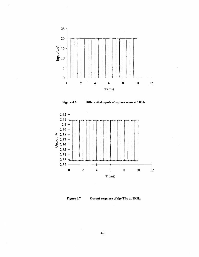
The output AC response of the TIA to the square wave inputs is studied at different
frequencies. An example of the differential inputs at 1KHz is shown in Figure 4.6. The
output responses at different frequencies are illustrated from Figure 4.7 to Figure 4.10.
When the frequency is below the bandwidth, the outputs keep square wave response and
the swing is 80mV. Thus the transimpedance gain is given by
(4.1)
When the frequency increases beyond the bandwidth, the waveform of the outputs
deviates from desired waveform. The reason is that the settling time is not small enough
with respect to the period of the input.
41
I
25
20
5
oo 2 4 6
T(ms)
8 10 12
Figure 4.6 Differential inputs of square wave at 1KHz
I
II
I
2.422.412.4
2.39~ 2.38
~ 2.37<5 2.36
2.352.342.332.32
o 2 4 6
T(ms)
8 10 12
Figure 4.7 Output response of the TIA at 1KHz
42

1.210.80.6
T (ms)
0.40.2
2.422.41
2.4
2.39,.-.,
G 2.38.....5. 2.37.....<5 2.36
2.352.342.332.32 +---+---f------+---+---+------1
o
Figure 4.8 Output response of the TIA at 10KHz
0.120.10.04 0.06 0.08
T (Jls)
l
0.02
2.42
2.412.4
2.39,.-.,
G 2.38
'[ 2.37
8 2.362.352.342.332.32 +---t------+---+---+----j---j
o
Figure 4.9 Output response of the TIA at 100MHz
43

35302515 20T (ns)
105
2.42
2.41
2.4
2.39
~ 2.38
8. 2.37
0= 2.36
2.35
2.34
2.33
2.32 +-------,---,-------,------,--,-------,-------.
o
Figure 4.10 Output response of the TIA at 400MHz
The fabricated TIA circuit is tested in order to verify the simulation results.
Figure 4.11 illustrates the experiment setup. Two differential voltage signals are
generated by the pulse wave generator as shown in Figure 4.12. The voltage swing is
4.02V. The duty cycle is 50%. The signals are fed into the nodes of input! and input2.
Each of them is placed in series with a resistor in order to create a current source. The
resistor value is 196kQ , in order to create a current swing of 20flA :
I . = Vswing
swmg R+R.m
4.02V :::: 20flA196kQ+5.2kQ
(4.1)
where Rin is the input impedance of the circuit. From the simulation results, we know the
input resistances of the resistive feedback TIA to be around 5.2kQ. Therefore the inputs
to the node of inl and in2 of the TIA can be viewed as square wave current sources,
which swing from 0 flA to 20 flA .
44

The output signals of the TIA, from the node of outl and out2, are filtered by a
capacitor in order to eliminate the high frequency noise. The filtered signals are sensed
by oscilloscope probes at the nodes of outputl and output2. The power supply probe and
the ground probe are used to provide a supply voltage of 5 volts and common ground to
the TIA circuit respectively. The breadboard is used for resistors, capacitors and common
ground connections. The measured experiment results are shown in the table and figures
below.
~~ 0
..0"0~
~~
0"0 ':::~"0 ::s ::s;> 0..0..
d d• ...-4 • ....-1
~ ........ : outputl. .: TIA :~----< gnd. .:. • .:I-I+,;,..,;,.,.;,------r--LJ 0 utput2
Chip
Figure 4.11 Resistive feedback TIA test setup
45

4.5
4
3.53
~ 2.5
I 2~ 1.5
1
0.5
o-0.5
-- -- ............. ....-...w- ............... r--""f
~~ r....--.......... -..... '-no' -1 2 3 4 5
T(ms)
Figure 4.12
DC operation
Differential signals generated by the pulse wave generator
The DC operation points of the experimental measurement are very close to those of
the simulation results. To evaluate, the relative error is given by
R I · E IReal Test Value -Simulation valuellOOOle ative rror = x -/0Simulation Value
(4.2)
All the relative errors mentioned later are calculated according to this equation. From the
data in Table 4.3, we notice that the relative error to be less than 0.8%. It indicates that
the TIA circuit works in the proper DC operation point in the experiment.
46

Nodes inl in2 out! out2
Simulation 2.323V 2.323V 2.368V 2.368V
Real Test 2.313V 2.316V 2.352V 2.355V
Relative Error 0.4% 0.3% 0.7% 0.5%
Table 4.3 Simulated and tested DC operation points of resistive feedback TIA
Output Response at Low Frequency and Transimpedance Gain
The AC output response of the TIA is tested at 1KHz and 10KHz, with the DC level
shifted to zero volt. The results are illustrated in Figure 4.13 and Figure 4.14. There is a
considerable amount of noise observed at the output nodes. We attribute this noise to the
experimental setup because the noise from the DC supply cannot be decoupled when
using DC probe. The output swing is approximately 70mV, whereas the simulation
suggested this value to be 80mV. Therefore, based on the experimental data, the
transimpedance gain is found to be 3.5kQ. As mentioned earlier, the AC measurement
was carried out only at low frequencies - use of DC probe and large parasitic
capacitances and inductances limit the measurement frequency.
47

5
60504030
---. 20~ 10'-"~ 0 +-----if---fr--t---ft---f-----ir---+--if------,
~-1Oo -20
-30-40-50-60
T(ms)
Figure 4.13 Outputs of the TIA at 1KHz
0.4
60504030
---. 20g 10~ 0 -f----Ift-----lI---i---i---t----I.--i---,
~-1Oo -20
-30-40-50-60
T(ms)
Figure 4.14 Outputs ofthe TIA at 10KHz
In order to improve the noise and bandwidth limitations caused by the measurement
set up, a PCB board was fabricated to test the packaged chip. Both the TIA and the front-
end amplifier were tested using an oscilloscope, model Agilent 54832D and probes,
48
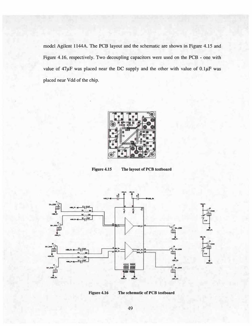
model Agilent 1144A. The PCB layout and the schematic are shown in Figure 4.15 and
Figure 4.16, respectively. Two decoupling capacitors were used on the PCB - one with
value of 47/lF was placed near the DC supply and the other with value of O.I/lF was
placed near Vdd of the chip.
Figure 4.15 The layout of PCB testboard
'I....,..
,.~-
~.. -J-.lLJ1'
'""'lJ' ..-...".
-.Jl'..'"'~~...sn.,..
•""'-"ll.
iiC....J'U•
..__.J
........
Figure 4.16 The schematic of PCB testboard
49

Bandwidth
The experimental and simulation results of TIA at different frequencies are shown in
Figure 4.17. The cutoff frequency of the amplifier is measured to be 27MHz. This is
considerably less than what was anticipated and was due to the low output impedance of
the amplifier and the loading effect of the probe. Because the TIA output resistance is
around 2.9 Kohm and the probe capacitance is 2pF, the output amplitude is limited by the
low output impedance at higher frequencies. Simulation of the TIA circuit with probe
capacitance as a load results in a bandwidth of 26 MHz, which is close to the value of the
bandwidth (24 MHz) measured.
Test- Simulation
100M1M10K100
45
40 i------------~
> 358';:;' 30 +-------------'0
.g 250..~ 20
"[ 15
<3 10
5
0+---------,--------,-------,------,-----------,
1
Frequency (Hz)
Figure 4.17 The output amplitude of TIA vs. frequency
Output Response at High Frequency and Transimpedance Gain
As shown in Figure 4.18 and Figure 4.19, the output noise is greatly reduced. The
noise amplitude using the PCB is around 5mV, whereas this value is more than lOmV in
50

the set up that involved using the breadboard. The output swing of the PCB test is 60mV.
Therefore, the transimpedance gain is 3ill. The response to the square wave input will
not distort until the frequency exceeds the bandwidth.
~JJ;j
fr -0.];jo
T(US}
0.3
Figure 4.18
Figure 4.19
Outputs of TIA at 10MHz
25
20
L -
- 0
-15
-20
-25
T us)
One output of TIA at 50MHz
51
0.3

4.2 Limiter Amplifier
The simulation schematic is shown in Figure 4.20. Two voltage sources are applied at
the two inputs nodes. They are biased at the DC level of 2.368V. This value is set
according to the DC level of outputs the TIA. The simulation results are illustrated in the
tables and figures below.
DC operation
Inl (V) In2 (V) Out (V)
2.368 2.368 2.377
Table 4.4 DC operation points of LA
Input and Output Resistance
The input resistance of LA is IT ohm, which is equal to 1012 ohm. It is very large
because the gate resistor of MOS is a very large.
Input Resistance (T ohm) 1
Output Resistance(K ohm) 107.1
Table 4.5 Input and Output Resistance of LA
52

Figure 4.20 The simulation schematic of the LA circuit
53

Input Voltage vs. Output Voltage
As shown in Figure 4.21, when the input swing exceeds lOmV, the output is non-
linear. It is because the second and the third stages of the LA operate in the saturation
region. This characteristic is expected in the LA circuit design and can be used as an
effective way to regulate the output signal of TIA. When TIA output is no longer a
perfect square waveform, the LA is able to regulate the input signal to be acceptable
square waveform. This regulation characteristic is further studied in the output response
of the limiter amplifier.
10080604020
4.5
4
3.5
3
2.5
2
1.5
1
0.5
0+-----,----,-----,----------.-------.
oPeak to Peak Input Voltage (mV)
Figure 4.21 The input voltage swing vs. output voltage swing of LA
Bandwidth
In order to ensure the LA linear operation, the input swing is set to be as small as 6mV.
Thus the output at different frequency can be plotted as shown in Figure 4.22. The
bandwidth estimated from simulation of the LA is 586.8MHz.
54

0.14r-..G 012
~ 0.1
~0.. 0.08
~ 0.06
~ 0.04.&S 0.02
O+---,.-~-r-----,..-------.-----r----,
1 O.lK 10K 1M
f(Hz)
100M 1G
Figure 4.22
Output Response and Output Swing
Voltage gain vs. Bandwidth
The output AC response of the LA is studied in two extreme cases. One case is when
the input signal is an ideal square wave as shown in Figure 4.23. The input swing is
80mV. The outputs are also square wave as shown in Figure 4.24, with a voltage swing
of 4.2V.
The other case is when the input signal is 80mV triangular wave as shown in Figure
4.25. Figure 4.26 shows that the output waveform has the resemblance of a square wave
with an output swing of 4.2V. Therefore, even when the output of the TIA may somewhat
deviate from the desired waveform due to limitations in its design, the output of the LA is
not severely impacted.
55

864
T (~s)
2
2.422.412.4
2.39>' 2.38'-'
E 2.37.E 2.36
2.352.342.332.32 +-----+-----1-------+------\
o
Figure 4.23 The square wave inputs of LA at IMHz
5
4
1
8.006.004.00
T (Ils)
2.00
O+---------i------+------+----~
0.00
Figure 4.24 The square wave outputs of LA at IMHz
56

7653 4
T (Ils)
21
2.42
2.41
2.4
2.39
;> 2.38'-"
~ 2.37p...s 2.36
2.35
2.34
2.332.32 -t-------,------.-----.------,------,--------,------,
o
Figure 4.25 The inputs of triangle waveform of the LA at IMHz
6543
T (Ils)
21
5
4.5
4
3.5;> 3'-"
8. 2.5:; 2o
1.51
0.5O+---+---+----+----+----t--------i
o
Figure 4.26 The outputs of LA at IMHz
57

4.3 Front-end Amplifier
The simulation schematic of the front-end amplifier is shown in Figure 4.27. The
setup is as the same as that of the TIA. The simulation results are illustrated in the tables
and figures below.
Figure 4.27 Simulation schematic of the front-end amplifier
58

DC operation
Table 4.6
inl (V) in2 (V) out (V)
2.168 2.168 2.261
Simulated Front-end Amplifier Operation Point
Input and Output Resistance
Input Resistance (K ohm)
Output Resistance (K ohm)
5.196
49.02
Table 4.7 Input and out resistance of front-end amplifier
Output Response and Output Swing
The output AC response of the front-end amplifier is studied at different frequencies,
as shown from Figure 4.28 to Figure 4.31. The output swing is 4.2V. It can be observed
that the waveform of the outputs keeps square wave when the frequency is below the
bandwidth of the TIA. When the frequency exceeds the bandwidth, the output waveform
exhibits distortion.
59

7653 4
T(ms)
21
54.5
43.5
,.-..,
G 3'[ 2.5.....8 2
1.5
10.5O+---t----+---+---+------1---+----i
o
Figure 4.28 Output response of front-end amplifier at 1KHz
54.5
4
3.5.-...;> 3'-"
8.. 2.5
8 21.5
1
0.5O+---f---+---f---+---f---+-----+----i
o 0.1 0.2 0.3 0.4 0.5
T (ms)
0.6 0.7 0.8
Figure 4.29 Output response of front-end amplifier at 10KHz
60

10080604020
54.5
43.5
,-..,
G 3
~ 2.5<3 2
1.5
10.5O+----+----f---------\-----+----j
oT (ns)
Figure 4.30 Output response of front-end amplifier at l00MHz
252015105
5
4.5
4
3.5,-..,
:> 3'--'.....6. 2.5E 2o
1.5
1
0.5O+----r--------,-------,-----,-------------,
oT(ns)
Figure 4.31 Output response of front-end amplifier at 500MHz
61

In order to verify the simulation results, the fabricated front-end amplifier circuit is
tested. The Figure 4.32 illustrates the experiment setup which is similar to the setup for
the TIA test as described above. The only difference is the output does not have a filter
capacitor. Because the front-end amplifier and the TIA have the same input resistance
value, the current inputs to the front-end amplifier are also square waves which swing
from OIlA to 20llA . The experiment results are shown in the tables and figures below.
output
in2inlR
R
i--------.········-----····
gndvdd
input!input2
...... ----_ _ .
BreadboardChip
Figure 4.32 Front-end amplifier test setup
DC operation
Table 4.8 displays the data of the DC operation points of the front-end amplifier. The
real test results are close to those of the simulation results because the absolute value of
the relative error is not larger than 3%. It indicates that the front-end amplifier works at
proper operation points.
62

inl in2 out
Simulation 2.168V 2.168V 2.261V
Real Test 2.235V 2.230V 2.33V
Relative Error 3% 3% 3%
Table 4.8 Simulated and tested DC operation points of front-end amplifier
Low Frequency Output Response
Figure 4.33 shows the test results of output response of front-end amplifier. The
output swing is approximately 4.1V. The relative error is 2%.
54321
5
4.5 -4
3.5,-."
:> 3'-"
'[ 2.5....<3 2
1.51
0.50+-------,---------,--------,--------,------,
oT(ms)
Figure 4.33 Output of front-end amplifier at 1KHz frequency
63

0.50.40.2 0.3
T(rns)
0.1
5
4.5
43.5
"""G 3.....5. 2.5.....8 2
1.51
0.5O+-------.------r-----i----------.---------,
o
Figure 4.34 Output of the front-end amplifier at 10KHz frequency
As previously mentioned, the PCB board test is performed to test the high frequency
performance of the front-end amplifier. Similar to the results of TIA discussed earlier, the
measured bandwidth is lower than anticipated because of the loading effect of probe
capacitance. As illustrated in Figure 4.35, experimental measurement and simulation,
which include the probe capacitance as the load, lead to bandwidth values of 1.6 MHz
and 1.5 MHz, respectively. Figure 4.36 and Figure 4.37 show the output response to
square wave inputs at two different frequencies.
64

4.5
4
3.5
0.5
--..---
- Simulation
-Test
0+----,-----,---,--------,-----,-------,,----;
1 10 100 1K 10K 100K 1M 10MFrequency (Hz)
Figure 4.35 Output swing of front-end amplifier vs. frequency
5
4.5
4
3.5
'""" 3>-'-'- 2.5:::I.9-:::I
20
1.5
1
-30 -20 -10 oT (us)
10 20 30
Figure 4.36 Outputs of front-end amplifier at 100KHz
65

3
2.2
2.1
-3 -2 -1 oT (us)
1 2 3
Figure 4.37
4.4 Inductive Peaking
Outputs of front-end amplifier at IMHz
The simulation setup for series inductive peaking is shown as Figure 4.38. The sources
are the same as the ones used for the resistive feedback TIA. While changing the
inductance value, the bandwidth is estimated and the result is illustrated in Figure 4.39.
When the inductance approaches lOJ-tH, the bandwidth is increased to 600MHz. However,
this is not a practical approach because the inductance value is too large for on chip
design.
66

inl .-----'I'"-H~4_+_l__---""'"'I1
ouf:1
Figure 4.38 Simulation schematic for series inductive peaking
650
600
,""",550N
~ 500£"0
~ 450§
r::Q 400
350
252015105
300 +------+-----+------+----+------1
oInductance(j.1lI)
Figure 4.39 Bandwidth enhancement vs. inductance by series inductive peaking
67

The same measurement on the series inductive peaking is performed. The simulation
schematic is displayed as Figure 4.40. As shown in Figure 4.41, the bandwidth is
440MHz when the inductance reaches 20nH. Therefore, the shunt inductive peaking can
be considered as an approach for future research for the TIA.
Figure 4.40 Simulation schematic of shunt inductive peaking
68

1000
900
~800
700'-'
<5'"0
~ 600§
I:Q 500
400
Figure 4.41
300 +--t--~--+--+---+--+--t--~--+---+-----1
0.00 0.10 0.20 0.30 0.40 0.50 0.60 0.70 0.80 0.90 1.00 1.10
Inductance (IlH)
Bandwidth enhancement vs. inductance by shunt inductive peaking
4.5 Summary
A summary of results is presented in Table 4.9. Whenever possible, the results from
simulation are validated through experimental measurements. Due to limitations in the
experimental setup, AC measurements have been limited to low frequencies. The
bandwidth parameter cannot be verified in the experiment. Inductive peaking is justified
at the simulation level. The benefits of inductive peaking are explored at the simulation
level. The shunt inductive peaking can be considered as an approach for future research
for the resistive feedback TIA circuit design, with significant potential enhancement in
the circuit's bandwidth.
69

Parameter Proposed Value Simulation Results Experiment Results
Data Rate 500Mb/s 535Mb/s N/A
TIA Bandwidth 350MHz 374.4MHz N/A
TIA Gain 3kQ 4kQ 3kQ
LA Bandwidth 450MHz 586.8MHz N/A
LA Output Swing 3.5V 4.2V 4.lV
Diode Light Current 20llA 20llA 20llA
Diode Capacitance 0.5pF 0.5pF 0.5pF
Table 4.9 The summary of the proposed values, simulation and experiment results
70

Chapter 5. Summary and Conclusion
The front-end amplifier, composed of a TIA and a LA, plays an important role in the
fiber optical system. The data rate of the optical system is largely determined by the
bandwidth, the transimpedance gain and the noise of the TIA. The LA circuit must boost
the output of the TIA to at least 250mV to drive the DMUX stage for data recovery.
In this thesis project, simulations for the TIA, the LA and the complete front-end
amplifier are conducted in the Cadence design environment cooperated with the NCSU
design kit. The TIA and the front-end amplifier is fabricated using the AMI
0.5 /.lm CMOS process. The test is performed using a probe station and breadboard to
verify the design.
Three design topologies including common-gate TIA, resistive feedback TIA and
capacitive feedback TIA are examined. The resistive feedback TIA is selected for the
thesis project design for two reasons. First, the resistive feedback TIA generates the
smallest noise among the three topologies. Second, the realization of the resistive
feedback TIA avoids using anyon-chip capacitor or inductor, which the AMI
0.5 /.lm CMOS process does not supply. The simulation results reveal that the estimated
bandwidth of the TIA is 374.4MHz and the transimpedance gain is 4 kQ . The
experimental determined transimpedance gain is 3 kQ .
The topology used to design the LA circuit is cascaded gain stages. There are three
gain stages used. The first two stages are the differential resistive load amplifiers. The
last stage is a buffer to convert the differential outputs to a single-end output. The
71

simulation results show that the bandwidth of the LA is 586.8MHz and the output swing
is 4.2V.
The complete front-end amplifier is implemented by cascading the TIA and the LA
together. According to the simulation data, the front-end amplifier achieves a data rate of
535Mb/s. The simulated output swing is 4.2V, while the experimental output swing
measured is found to be s 4.1V. Due to the constraints of the probe load effect, the
functionality of the two circuits is demonstrated up to 20MHz. Designing a buffer at the
end of the TIA and the front-end amplifier to transfer the impedance to 50 ohm may
enable the test to go up to GHz frequency range.
The technique of inductive peaking for enhancing the bandwidth of a TIA is also
explored through simulation. The simulation results reveal that the shunt inductive
peaking may help increase the bandwidth of the circuit and may be considered for future
development of CMOS-based TIA design.
72

References
1 W. Chen and C. Lu, "A 2.5 Gbps CMOS Optical Receive Analog Front-end",
IEEE Custom Integrated Circuits Conference, May 2002, pp. 359-362.
2 A.K. Petersen, K. Kiziloglu, T. Yoon, F. Williams, and M.R. Sandor, "Front-end
CMOS Chipset for 10 Gb/s Communication", IEEE Radio Frequency Integrated
Circuits Symposium, June 2002, pp. 93-96.
3 Behzad Razavi, Design of Integrated Circuits for Optical Communications,
McGraw-Hill Press, 2003.
4 M. Ingels and S.J.S. Steyaert, "A I-Gb/s, 0.7um CMOS Optical Receiver with
Full Rail-to Rail Output Swing", IEEE Journal of Solid-state Circuits, Vol. 34,
July 1999, pp. 971-977.
5 M. Jaime and D. Alejandro, "Differential Transimpedance Amplifiers for
Communications Systems Based on Common-gate Topology", Fourth IEEE
International Caracas Conference on Devices, Circuits and Systems, April 2002,
pp. C027-1 - C027-4.
6 M. Jaime, D. Alejandro Jaime and L. Monico, "Differential Transimpedance
Amplifiers for Communications Systems Based on Common-gate Topology",
73

IEEE International Symposium on Circuits and Systems, Vol. 2, May 2002, pp. II
97 - II -100.
7 Apsel and Andreou, "5mW, Git/s silicon on sapphire CMOS optical receiver",
Electronics letters, Vol. 37, September 2001, pp. 1186-1188.
8 H. Hamano, T. Yamamoto, el., "High-speed Si-bipolar IC design for multi-Gb/s
optical receivers", IEEE Journal on Selected Areas in Communications, Vol. 9,
June 1991, pp. 645-651.
9 A. Jaakuma , M.S. Bustos, el. , "3-V MSM-TIA for Gigabit Ethernet", IEEE
Journal ofSolid-State Circuits, Vol. 35, September 2000, pp. 1271-1275.
10 Amit Gupta, Investigation of High-speed Optoelectronic Receivers in Silicon
Germanium (Sil-xGex).
11 C. Rooman, D. Coppee, el. "Asynchronous 250-Mb/s Optical Receiver with
Integrated Detector in Standard CMOS Technology for Optocoupler
Applications", IEEE Journal of Solid-state Circuits, Vol. 35, July 2000, pp. 953
958.
12 Carlos Roberto Calvo, A 2.5 GHz Optoelectronic Amplifier in 0.18 11m CMOS
13 S.S. Taylor and T.P. Thomas, "A 2 pAl.JHz 622Mb/s GaAs MESFET
Transimpedance Amplifier", ISSCC Digest of Technical Papers, February 1994,
pp. 254-255.
74

14 A. Apsel, A.G. Andreou, and J. Liu, "A 6 Channel Array of a 5 Milliwatt,
500MHz Optical Receivers in 0.5um SOS CMOS", IEEE International
Sysmposium on Circuits and Systems, Vol. 5, May 2002, pp. V-433 - V-436.
15 B. Razavi., "A 622Mb/s, 4.5 pA/~Hz CMOS Tranimpedance Amplifier", ISSCC
Digest ofTechnical Papers, February 2000, pp.162-163.
16 S.S. Mohan, M.M. Hershenson, S.P. Boyd, and T.H. Lee, "Bandwidth Extension
in CMOS with Optimized On-chip Inductors", IEEE Journal of Solid-State
Circuits, Vol. 35, March 2000, pp. 346-355.
17 K. Schrodinger, J. Simma, and M. Mauthe, "A fully integrated CMOS Receiver
Front-end fr Optical Gigabit Ethernet", IEEE Journal ofSolid-State Circuits, Vol.
37, July 2002, pp. 874-880.
75


