
10/13/2005 Copyright 2004 S.D. Sudhoff Page 5
2 / QD Models for Permanent Magnet Synchronous Machines The objective of this chapter is to derive lumped parameter models for permanent magnet synchronous machines. This development will begin by setting forth the assumed configuration and some preliminary definitions in Section 2.1. This is followed by a derivation of the machine model in abc variables in Section 2.2. Next, Section 2.3 focuses on the transformation of the abc variable model to qd0 variables. This transformation result in considerable simplification of the model by eliminating rotor position dependence. Using the qd0 model, the steady-state performance of the machine is described in Section 2.4. Section 2.5 describes a procedure to measure the parameters of the standard qd0 model. Time domain simulation using the model is discussed in Section 2.6. Therein, some discrepancies between model predictions and observed performance will be noted. To address these, an improved qd0 model is described in Section 2.7; the parameterization of this model is described in Section 2.8.
2.1 PRELIMINARIES In this chapter, lumped parameter models for PMSM machines are developed. In order to derive these models, we will assume the configuration shown in Fig 2.1-1. This machine is a radial airgap, surface mounted permanent magnet machine. A 2-pole machine is shown in Fig. 2.1-1; however any even number of poles may be readily obtained.
q-axis
d-axis
as-axis
bs-axis
cs-axis
rmθ
smφ
rmφ
Stator
RotorCore
PermanentMagnet
StatorSlot
Shaft
Spacer
Figure 2.1-2. Permanent Magnet Synchronous Machine.

10/13/2005 Copyright 2004 S.D. Sudhoff Page 6
The as-, bs-, and cs-axis mark the direction of positive flux through the center of the machine as caused by the a-, b-, and c- phase currents, respectfully. The d-axis marks the North magnetic pole of the permanent magnet; the q-axis is orthogonal to the poles. The angle from the as-axis to the q-axis is defined as the mechanical rotor position rmθ (in the two pole case). Angular position as measured from the stator is measured relative to the as axis and is denoted smφ . Angular position as measured from the rotor is measure relative to the q-axis and is designated rmφ . If we are describing the same feature using the two different coordinate systems (stator and rotor) observe that we must have rmrmsm φθφ += (2.1-1) In treating machines with more than two pole pairs it is convenient to define electrical rotor position and speed. These quantities are defined as
rmrP θθ2
= (2.1-2)
rmrP ωω2
= (2.1-3)
where P is the number of poles. Clearly, for a 2 pole machine the electrical and mechanical quantities are identical. It is also convenient to define electrical stator and rotor position as
smsP φφ2
= (2.1-4)
rmrP φφ2
= (2.1-5)
From (2.1-1)-(2.1-5), rrs φθφ += (2.1-6) It will be assumed that the machine has sinusoidally distributed windings. In particular, it is assumed that the stator turns density may be expressed ( )spsmas nn φφ sin)( = (2.1-7)
( )3/2sin)( πφφ −= spsmbs nn (2.1-8)
( )3/2sin)( πφφ += spsmcs nn (2.1-9) It follows from Chapter 4 of [1] that the winding functions may be expressed

10/13/2005 Copyright 2004 S.D. Sudhoff Page 7
( )sp
sas Pn
w φφ cos2
)( = (2.1-10)
( )3/2cos2
)( πφφ −= sp
sbs Pn
w (2.1-11)
( )3/2cos2
)( πφφ += sp
scs Pn
w (2.1-12)
In deriving (2.1-10)-(2.1-12), it should be recalled that the integration involved in computing winding functions from turns density is in terms of mechanical rather than electrical rotor position; the result is the P/2 factor in the winding functions.
One feature of particular interest in Fig. 2.1-1 is the spacer; we will consider this to be either an inert material with a relative permeability of unity, or it could be the same magnet steel that is used for the rotor. As we will see, the choice of spacer material will make a significant impact on the performance characteristics of the machine.
2.2 ABC MODEL There are essentially three components of the model of any electromechanical device – a voltage equation, a flux linkage equation, and a torque equation. We begin our discussion of the abc variable machine model with the voltage equation. By Ohm’s and Faraday’s laws, the voltage across each phase will be equal to the Ohmic drop across that phase plus the time rate of change of flux linkage. In vector form, we have
abcsabcssabcs pr λiv += (2.2-1) In (2.2-1) the stator resistance is readily established in terms of the machine geometry using techniques set forth in Section 4.8 of [1]. The next step in formulating the machine model is to formulate the flux linkage equation. The flux linking each phase may be thought of as having two components, a leakage component which does not cross the air gap and a magnetizing component which does. Thus mabcslabcsabcs ,, λλλ += (2.2-2) where labcs,λ and mabcs,λ denote the leakage and magnetizing components, respectively. From our work in Section 4.7 of [1], we have
10/13/2005 Copyright 2004 S.D. Sudhoff Page 8
abcs
lplmlm
lmlplm
lmlmlp
labcsLLLLLLLLL
iλ⎥⎥⎥
⎦
⎤
⎢⎢⎢
⎣
⎡
=, (2.2-3)
where lpL and lmL can be calculated in terms of the machine geometry using the methods set forth in Section 4.7 of [1]. In order to calculate the magnetizing component of the flux linkage, let us specifically consider the a-phase magnetizing flux linkage. From Section 4.6 of [1], the a-phase flux linkage may be expressed
∫=π
φφφλ2
0, )()( smsssasmas ddrBw (2.2-4)
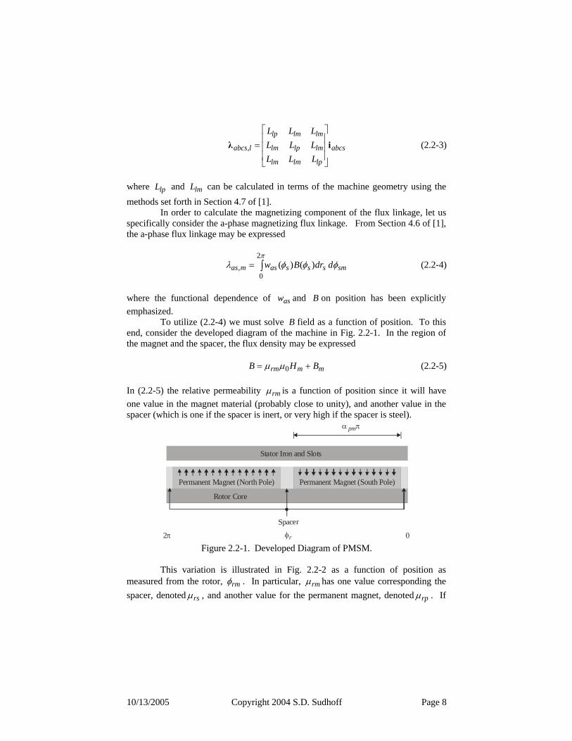
where the functional dependence of asw and B on position has been explicitly emphasized. To utilize (2.2-4) we must solve B field as a function of position. To this end, consider the developed diagram of the machine in Fig. 2.2-1. In the region of the magnet and the spacer, the flux density may be expressed mmrm BHB += 0µµ (2.2-5) In (2.2-5) the relative permeability rmµ is a function of position since it will have one value in the magnet material (probably close to unity), and another value in the spacer (which is one if the spacer is inert, or very high if the spacer is steel).
0π2
Permanent Magnet (North Pole) Permanent Magnet (South Pole)
Spacer
Stator Iron and Slots
Rotor Core
rφ
πα pm
Figure 2.2-1. Developed Diagram of PMSM.
This variation is illustrated in Fig. 2.2-2 as a function of position as measured from the rotor, rmφ . In particular, rmµ has one value corresponding the spacer, denoted rsµ , and another value for the permanent magnet, denoted rpµ . If

10/13/2005 Copyright 2004 S.D. Sudhoff Page 9
the spacer is steel, rsµ is much greater than rpµ . If the spacer is inert, rsµ is unity
and slightly less than rpµ . Fig. 2.2-1 also depicts the variation of mB with position;
therein pmB denotes the residual flux density of the magnet. In the air gap, we must have
gHB 0µ= (2.2-6)
0π2
pmB πα pm
rφ
mB
rmµrsµ rpµ
Figure 2.2-2. Developed Diagram Showing Magnet and Spacer Properties.
At a given position, the B field values in (2.2-5) and (2.2-6) must be the same. Combining (2.2-5) and (2.2-6) yields an expression for the field intensity in the material (permanent magnet or spacer), mH , in terms of the field intensity in the air gap, gH , and the flux density do to the material mB .
⎟⎟⎠
⎞⎜⎜⎝
⎛−= m
og
rmm BHH
µµ11 (2.2-7)
The definition of MMF drop is that
∫=stator
rotorHdrF (2.2-8)
where we will take the rotor to be the rotor core. From (2.2-8), mmg dHgHF += (2.2-9) Manipulation of (2.2-6), (2.2-7) and (2.2-9) yields effmbf BFcB ,+= (2.2-10) where

10/13/2005 Copyright 2004 S.D. Sudhoff Page 10
mrm
rmbf dg
c+
=µ
µµ0 (2.2-11)
and
mmrm
meffm B
dgdB
+=
µ, (2.2-12)
Because rmµ and mB are functions of position, it follows that bfc and
effmB , will be a function of position as well. This is depicted in Fig. 2.2-3. Therein,
mrs
rsbfs dg
c+
=µ
µµ0 (2.2-13)
mrp
rpbfm dg
c+
=µ
µµ0 (2.2-14)
and
pmmrp
meffpm B
dgdB
+=
µ, (2.2-15)
0π2
πα pm
rφ
effmB ,
bfc
effpmB ,
bfsc bfmc
Figure 2.2-3. Developed Diagram Showing Effective Properties.
At this time, all terms in (2.2-10) have been specified accept for the MMF drop from the rotor core to the stator. We have cscsbsbsasas iwiwiwF ++= (2.2-16) Substitution of (2.2-16) into (2.2-10) and the result into (2.2-4) yields
( )( )∫ +++=π
φλ2
0,, smeffmcscsbsbsasasbfassmas dBiwiwiwcwdr (2.2-17)
In the process of evaluating (2.2-17), observe that it is somewhat awkward to express bfc and effmB , in terms of stator position since these quantities are

10/13/2005 Copyright 2004 S.D. Sudhoff Page 11
associated with the rotor. Since it is relatively straightforward to express the winding function in terms of rmrm θφ + (which is equal to smφ ), it is convenient to express (2.2-17) as
( )( )∫ +++=π
φλ2
0,, rmeffmcscsbsbsasasbfassmas dBiwiwiwcwdr (2.2-18)
A further reduction can be obtained by using symmetry to evaluate (2.2-18)
over one pole pair and multiplying the result by the number of poles pairs 2/P . In addition, because the integrand must be an even function, it is only necessary to integrate over one pole face if we multiply the resulting quantity by an additional factor of two. This yields
( )( )∫ +++=P
rmeffmcscsbsbsasasbfassmas dBiwiwiwcwPdr/2
0,,
πφλ (2.2-19)
Evaluating (2.2-19) yields
pmascsascsbsasbsasasasmas iLiLiL ,, λλ +++= (2.2-20) where
∫=π
φ0
2 rbfyassasy dcwwdrL (2.2-21)
and
∫=π
φλ0
,, 2 reffmasspmas dBwdr (2.2-22)
In (2.2-21), ‘y’ may each take on values of ‘as’, ‘bs’, and ‘cs’. It remains, of course, to actually evaluate (2.2-21) and (2.2-22). Expanding (2.2-21) yields,
⎥⎥⎥⎥
⎦
⎤
⎢⎢⎢⎢
⎣
⎡
−+= ∫ ∫+
−
ππα
πα
φφ0
)1(21
)1(21
)(2pm
pm
ryasbfsbfmryasbfssasy dwwccdwwcdrL (2.2-23)
Let us first use (2.2-23) to compute asasL . Substiution of (2.1-10) into (2.2-23) for asw and yw yields
( )[ ])2cos()sin()(4
2
2
rpmpmbfsbfmbfsps
asas cccP
ndrL θπαπαπ −−+= (2.2-24)

10/13/2005 Copyright 2004 S.D. Sudhoff Page 12
which may be expressed )2cos( rBAasas LLL θ+= (2.2-25) where
( ))(4
2
2
bfsbfmpmbfssp
A cccP
drnL −+= α
π (2.2-26)
and
)sin()(42 pmbfmbfss
B ccPdrL πα−= (2.2-27)
Next, we will use (2.2-23) to compute asbsL . Substitution of (2.1-10) and (2.1-11) into (2.2-23) yields
⎥⎦
⎤⎢⎣
⎡⎟⎟⎠
⎞⎜⎜⎝
⎛⎟⎠⎞
⎜⎝⎛ +−−+−=
32cos)sin(2)(
22
2 πθπαπαπ rpmpmbfsbfmbfsps
asbs cccP
ndrL
(2.2-28) which is readily expressed
⎟⎠⎞
⎜⎝⎛ ++−=
32cos
21 πθrBAasbs LLL (2.2-29)
Following the same procedure, it can be shown that
⎟⎠⎞
⎜⎝⎛ −+−=
32cos
21 πθrBAascs LLL (2.2-30)
We next turn our attention to (2.2-22). Substitution of the winding function into the integrand and evaluating yields )sin(, rmpmas θλλ = (2.2-31) where
mrm
mpmpmspm dg
dP
Bdrn+⎟⎟
⎠
⎞⎜⎜⎝
⎛=
µπα
λ2
sin8
(2.2-32)
At this point, we have computed all terms related to a-phase magnetizing flux linkage. Repeating the process for the b- and c-phases yields

10/13/2005 Copyright 2004 S.D. Sudhoff Page 13
( )
⎥⎥⎥
⎦
⎤
⎢⎢⎢
⎣
⎡
+−
+⎥⎥⎥
⎦
⎤
⎢⎢⎢
⎣
⎡
−−++
−+
+⎥⎥⎥
⎦
⎤
⎢⎢⎢
⎣
⎡
−−−−−−
=
)3/2sin()3/2sin(
)sin(
)3/22cos()2cos()3/2cos()2cos()3/22cos()3/2cos(
)3/2cos(3/2cos)2cos(
211121112
2,
πθπθ
θλ
πθθπθθπθπθ
πθπθθ
r
r
r
m
abcs
rrr
rrr
rrr
B
abcsA
mabcs
L
L
i
iλ
(2.2-33)
which completes our derivation of the flux linkage equations. At this point, we could use co-energy techniques to formulate an expression for torque. However, we will defer this derivation until the next section wherein the qd0 model is set forth. As a final note, note that the stator slot effects will cause the effective air gap to be greater than the physical gap g . For this reason, it is recommend to adjust replace g with an effective value which may be obtained using Carter’s coefficient as discussed in Section 4.6.2 of [1].
2.3 STANDARD QD0 MODEL The ABC machine model flux linkage equations are complex. The matrices used have both diagonal and off-diagonal elements, and are a function of rotor position. Significant simplification can be brought about by transforming the variables to the rotor reference frame. In particular, we will define qd0 variables which are related to abc variables by the transformation abcs
rs
rsqd fKf =0 (2.3-1)
where abcsf is a vector of abc variables of the form [ ]Tcsbsasabcs fff=f (2.3-2) and r
sqd 0f is a vector of qd0 variables defined as
[ ]Tsr
dsr
qsr
sqd fff 00 =f (2.3-3) and where f may denote a voltage, current, or flux linkage. Recall from Chapter 2 of [1] that

10/13/2005 Copyright 2004 S.D. Sudhoff Page 14
⎥⎥⎥⎥⎥
⎦
⎤
⎢⎢⎢⎢⎢
⎣
⎡
+−+−
=
21
21
21
)`3/2cos()3/2sin()sin()3/2cos()3/2cos()cos(
32 πθπθθ
πθπθθ
rrr
rrrrsK (2.3-4)
Applying (2.3-1) to the voltage equation (2.2-1) yields the qd0 voltage equation r
sqdr
sqdrr
sqdsr
sqd pr 0000 λSλiv ++= ω (2.3-5) where S is the speed coefficient matrix
⎥⎥⎥
⎦
⎤
⎢⎢⎢
⎣
⎡−=
000001010
S (2.3-6)
Transforming (2.2-2) to the rotor reference frame yields r
msqdr
lsqdr
sqd ,0,00 λλλ += (2.3-7)
The leakage flux linkage term r
lsqd ,0λ may be obtained by transformation of (2.2-3):
rsqdls
lsr
lsqdL
LL
0
0
,000
0000iλ
⎥⎥⎥
⎦
⎤
⎢⎢⎢
⎣
⎡= (2.3-8)
In (2.3-8) lmlpls LLL −= (2.3-9) lmlp LLL 20 += (2.3-10) The magnetizing component of the flux linkage in (2.3-7) is found by transforming (2.2-33). This yields
⎥⎥⎥
⎦
⎤
⎢⎢⎢
⎣
⎡+
⎥⎥⎥
⎦
⎤
⎢⎢⎢
⎣
⎡−+
⎥⎥⎥
⎦
⎤
⎢⎢⎢
⎣
⎡=
000
000010001
23
000010001
23
00,0 mr
sqdBr
sqdAr
msqd LL λiiλ (2.3-11)
It is convenient to combine terms in (2.3-11) as
10/13/2005 Copyright 2004 S.D. Sudhoff Page 15
⎥⎥⎥
⎦
⎤
⎢⎢⎢
⎣
⎡+
⎥⎥⎥
⎦
⎤
⎢⎢⎢
⎣
⎡=
010
000000
0
0
0 mr
sqdd
qr
sqdL
LL
λiλ (2.3-12)
where
)(23
BAlsq LLLL ++= (2.3-13)
( )BAlsd LLLL −+= 2
3 (2.3-14) At this point we have a voltage equation (2.3-5) and flux linkage equation (2.3-12). To complete the model, we must have an expression for electromagnetic torque. From our work in Chapter 5 of [1], we have that
( )rds
rqs
rqs
rdse iiPT λλ −=
223 (2.3-15)
Together, the three equations (2.3-5), (2.3-12), and (2.3-15) make up the standard qd0 machine model.
2.4 STEADY STATE OPERATION Under sinusoidal steady-state conditions in the rotor reference frame, all variables are constant. Thus we may set all derivative terms in the voltage equation (2.3-5) equal to zero. Taking this result, combining it with the flux linkage equation (2.3-12), and separating out the q- and d-axis components yields mr
rdsdr
rqss
rqs iLirv λωω ++= (2.4-1)
rqsqr
rdss
rds iLirv ω−= (2.4-2)
The zero-sequence voltage equation is not considered since in all zero sequence quantities must be zero in an idealized machine, whether it be delta- or wye-connected. For the purposes of steady-state analysis, it is convenient to substitute the flux linkage equation (2.3-12) into the torque equation (2.3-15) to yield
( )rds
rqsqd
rqsme iiLLiPT )(
223
−+= λ (2.4-3)
It should be observed that this result is valid for steady-state or transient conditions. Together, (2.4-1)-(2.4-2) and (2.4-3) constitute the steady-state PMSM

10/13/2005 Copyright 2004 S.D. Sudhoff Page 16
model. In order to demonstrate the use of the model, let us assume the case that the machine is supplied from a three-phase controllable voltage source (i.e. an inverter) and that the phase voltages have the form )cos(2 vrsas vv φθ += (2.4-4)
)3/cos(2 vrsbs vv φπθ +2−= (2.4-5)
)3/2cos(2 vrscs vv φπθ ++= (2.4-6) Transforming these voltages to the rotor reference frame yields )cos(2 vs
rqs vv φ= (2.4-7)
)sin(2 vsrds vv φ−= (2.4-8)
Given the voltages, (2.4-1) and (2.4-2) may be solved to find the currents. In particular, we have
qdrs
drmrrqssr
qsLLr
Lvri 22
)(
ω
ωλω
+
−−= (2.4-9)
qdrs
rdssmr
rdsqrr
dsLLr
vrvLi 22
)(
ω
λωω
+
+−= (2.4-10)
These currents can then be substituted into (2.4-3) to find the torque. As an alternative to controlling the machine voltage, it is also possible to control the current. In fact, this is the normal case for all but the lowest power machines. In this case the stator currents are controlled to be of the form )cos(2 irsas ii φθ += (2.4-11)
)3/2cos(2 irsbs ii φπθ +−= (2.4-12)
)3/2cos(2 irscs ii φπθ ++= (2.4-13) which corresponds to )cos(2 is
rqs ii φ= (2.4-14)
)sin(2 isrds ii φ−= (2.4-15)
Using (2.4-14)-(2.4-15) may be used in conjunction with (2.4-3) to find the torque. The q- and d-axis machine voltage can be found from (2.4-1) and (2.4-2) and the torque using (2.4-3).

10/13/2005 Copyright 2004 S.D. Sudhoff Page 17
When operating the machine from a voltage source, it useful to note that from (2.4-14) and (2.4-15) the per phase rms stator current may be expressed
( ) ( )22
21 r
dsrqss iii += (2.4-16)
Similarly, when operating the machine from a current source, from (2.4-7) and (2.4-8) the line-to-neutral rms stator voltage may be expressed
( ) ( )22
21 r
dsrqss vvv += (2.4-17)
One the voltages, currents, and torque is computed output power is the product of torque and mechanical rotor speed; thus
erout TP
P ω2= (2.4-18)
From our work in Chapter 2 of [1], we have that the input power may be expressed
( )rds
rds
rqs
rqsin ivivP +=
23 (2.4-19)
Finally, the efficiency (in percent) may be found in accordance with
⎪⎪⎪
⎩
⎪⎪⎪
⎨
⎧
<>
≤<
>≥
=
0,00
0,0
0,0
outin
inoutout
in
inoutin
out
PP
PPPP
PPPP
η (2.4-20)
where the three difference cases arise based on the direction of power flow. It is now appropriate to consider a numerical example. Let us consider a commercial 3-phase 4-pole machine rated for 1 Hp at a speed of 2000 rpm; and a maximum operating speed of 5500 rpm. Rated current for this machine is 3.3 A rms; rated torque is 3.56 Nm. The machine parameters are =sr 2.6 Ω, == dq LL 12.4 mH, and =mλ 0.286 Vs. Figure 2.4-1 illustrates machine performance versus speed wherein the input voltage is fixed at 230 V, l-l, rms and the phase advance is zero. All quantities are normalized to their rated value, where rated power is taken to be 746 W; 100% efficiency corresponds to 10 in the figure.

10/13/2005 Copyright 2004 S.D. Sudhoff Page 18
0 500 1000 1500 2000 2500 3000 3500 4000 4500 5000 5500-20
-10
0
10
20
30
40
ωrm, RPM
per u
nit
isTe
PinPout
η*10
Figure 2.4-1. Steady-State Operation From A Voltage Source.
As can be seen, at low speeds the input current, torque, and input power are extremely high (15, 17, and 27 time rated value, respectively). Output power is low since the speed is low. As the speed increases, the input current, torque, and input power decrease; the output power increases rapidly with speed and eventually the efficiency enters an acceptable range. At approximately 3100 rpm, the torque drops below zero and the machine begins to acts as a generator. The large input currents illustrate the disadvantage of fixed amplitude voltage source control; it is entirely inappropriate for this class of machine. Figure 2.4-2 illustrates performance with current source control. In this case, the machine is operated with a current command equal to its rated value and
iφ equal to zero. As can be seen, the machine performance is quite good over the entire speed range. An extended discussion of current based control is set forth in Chapter 3.

10/13/2005 Copyright 2004 S.D. Sudhoff Page 19
0 500 1000 1500 2000 2500 3000 3500 4000 4500 5000 55000
0.5
1
1.5
2
2.5
3
3.5
ωrm, RPM
per u
nit
vs
Te
PinPout
η
Figure 2.4-2. Steady-State Operation From a Current Source.
2.5 PARAMETER IDENTIFICATION While we established expressions for the parameters of the machine in Section 2.2, it is often the case that it is desirable to measure the parameters directly. In this section, a procedure to identify the machine parameters is set forth. Herein, it is assumed that the machine is wye- connected. Modifications for delta-connected machines are straightforward. The first step in the procedure identifies mλ , and, if not already known, the number of poles P . The experimental set up involves driving the machine under test mechanically from a dynamometer at a safe operating speed for the device. During this test, the machine is open circuited, and the a- to b- phase voltage abv is measured. From (2.4-1)-(2.4-2) we have
⎥⎥⎥
⎦
⎤
⎢⎢⎢
⎣
⎡=
001
0 mrr
sqd λωv (2.5-1)
which, when transformed back to abc variables, yields

10/13/2005 Copyright 2004 S.D. Sudhoff Page 20
⎥⎥⎥
⎦
⎤
⎢⎢⎢
⎣
⎡
+−=
)3/2cos()3/2cos(
)cos(
πθπθ
θλω
r
r
r
mrabcsv (2.5-2)
From (2.5-2), it can be shown that the a- to b- phase voltage may be expressed )6/cos(3 πθλω += rmrabsv (2.5-3) Since the machine is being driven at a constant speed, we may express the rotor position as 0rrr t θωθ += (2.5-4) where 0rθ is a constant. Thus, (2.5-4) becomes )6/cos(3 0 πθωλω ++= rrmrabcs tv (2.5-5) Observe that rω is known as it corresponds to the radian frequency of the observed line-to-line voltage. From (2.5-5) we have that
r
fndpkabcsm
v
ωλ
3= (2.5-6)
where fundpkabsv denotes the peak value of the fundamental component of the a- to
b-phase voltage. If the number of poles is unknown, it may be readily calculated if the mechanical rotor speed is known. In particular, from (2.1-3) )/(2 rmrroundP ωω= (2.5-7) In (2.5-7) the ()round operator rounds the result to the nearest integer. The next step in the procedure is to identify the stator resistance and d-axis inductance. This will be accomplished using stand still impedance testing using the configuration shown in Fig. 2.5-1. Therein, the impedance meter (often referred to as an LCR meter), applies a small signal ac voltage at a frequency ω , measures the applied voltage and resulting current waveforms and then proceeds to compute and report the observed impedance mZ at frequency ω . Often, such devices will feature the ability to provide a dc voltage and current offset to bias to the device under test.

10/13/2005 Copyright 2004 S.D. Sudhoff Page 21
ImpedanceMeter
+
-
a
b c
abv
asi
as
abm i
vZ ~
~=
Figure 2.5-1. D-axis parameter measurement set up.
Before measuring the impedance, we first position the rotor to 2/πθ =r . If the machine is equipped with a calibrated rotor position sensor, this is straightforward. If the machine does not have a rotor position sensor, then the rotor may be positioned by connecting the b- and c-phase currents together, and then injecting a positive dc current into the a-phase (with a magnitude less than the rated peak value of current into the machine). The resulting stator field will be in the direction of the positive as axis. The d-axis of the rotor will align with the stator field, at which point rθ = 2/π . The rotor is then mechanically locked into this position. Note that the d-axis voltage may be expressed
( ))3/2sin()3/2sin()sin(32 πθπθθ ++−+= rcsrbsras
rds vvvv (2.5-8)
which, at 2/πθ =r reduces to
⎟⎠⎞
⎜⎝⎛ −−= csbsas
rds vvvv
21
21
32 (2.5-9)
which may also be expressed as
⎟⎠⎞
⎜⎝⎛ −+−= )(
21)(
21
32
csasbsasrds vvvvv (2.5-10)
Since the b- and c-phases are connected together abac vv = and thus
abrds vv
32
= (2.5-11)
The d-axis current may be expressed
( ))3/2sin()3/2sin()sin(32 πθπθθ ++−+= rcsrbsras
rds iiii (2.5-12)
which, at 2/πθ =r , reduces to
⎟⎠⎞
⎜⎝⎛ −−= csbsas
rds iiii
21
21
32 (2.5-13)

10/13/2005 Copyright 2004 S.D. Sudhoff Page 22
Since the machine is assumed to be wye-connected ascsbs iii −=+ (2.5-14) Substitution of (2.5-14) into (2.5-13) yields as
rds ii = (2.5-15)
We now define the standstill impedance looking into the d-axis of the machine as
rds
rds
div
Z ~~
= (2.5-16)
Since (2.5-11) and (2.5-15) hold for instantaneous quantities under stand still conditions, they also hold for phasor quantities. Substitution of these two relationships into (2.5-16) yields
mas
abd Z
iv
Z32
~~
32
== (2.5-17)
where mZ is the impedance reported by the impedance meter. Observe that setting 0=rω in the d-axis voltage equation, and combining it with the d-axis flux linkage equation, we have that r
dsdrdss
rds piLirv += (2.5-18)
From (2.5-18), it is clear that dsd LjrZ ω+= (2.5-19) where ω is the frequency of the injected perturbation. Thus we have )Re( ds Zr = (2.5-20)
)Im(1dd ZL
ω= (2.5-21)
The final step in the procedure is to calculate the q-axis parameters. To this end, it is convenient to leave the rotor locked in the same position as the previous step, but to connect our test source from the b-phase to the c-phase, with the a-phase open circuited. This configuration is depicted in Figure 2.5-1. The q-axis voltage equation may be expressed

10/13/2005 Copyright 2004 S.D. Sudhoff Page 23
ImpedanceMeter
+
-a
b
c
bs
bcm i
vZ ~
~=
bsi
bcv
Figure 2.5-2. Q-Axis parameter measurement set up.
( ))3/2cos()3/2cos()cos(32 πθπθθ ++−+= rcsrbsras
rqs vvvv (2.5-22)
Setting 2/πθ =r in (2.5-22) yields
⎟⎟⎠
⎞⎜⎜⎝
⎛−= csbs
rqs vvv
23
23
32 (2.5-23)
Thus,
bcrqs vv
31
= (2.5-24)
The q-axis current may be expressed
( ))3/2cos()3/2cos()cos(32 πθπθθ ++−+= rcsrbsras
rqs iiii (2.5-25)
which, upon setting 2/πθ =r , yields
⎟⎟⎠
⎞⎜⎜⎝
⎛−= csbs
rqs iii
23
23
32 (2.5-26)
Since the a-phase is open circuited, bscs ii −= and so
bsrqs ii
332
= (2.5-27)
The q-axis stand-still impedance is defined as

10/13/2005 Copyright 2004 S.D. Sudhoff Page 24
rqs
rqs
qi
vZ ~
~= (2.5-28)
From (2.5-24) and (2.5-28) we have that
mas
abq Z
iv
Z21
~~
21
== (2.5-29)
Substitution of the q-axis flux linkage equation into the q-axis voltage equation for zero speed conditions yields r
qsqrqss
rqs piLirv += (2.5-30)
Thus qsq LjrZ ω+= (2.5-31) and
)Re(1qq ZL
ω= (2.5-32)
Using the procedure set forth, the calculation of the parameters may seem clear. In particular, once a perturbation frequency is selected (2.5-20), (2.5-21), and (2.5-32) can be used to find sr , dL , and qL , respectfully. However, there are some subtle points which must be considered. The first of these is that, as mentioned previously, most impedance meters are capable of providing a dc bias, which raises the issue of what bias level should be used. If the machine had truly linear magnetics, this would not be an issue. However, no machine has linear magnetics and so it is. In the case of the d-axis, zero bias is a good starting point since it is often the case that the d-axis current will be zero. In the case of the q-axis, it may be reasonable to injected a q-axis current corresponding to the rated current of the machine; subject to limitations of the LCR meter. In addition to the bias level, the size of the perturbation used can also have an effect. If to small a bias is used, minor-loop hysteresis effects will come into play and cause a condition in which the measured impedance is a function of perturbation level. If to large a perturbation is used, nonlinearities in the flux linkage versus current relationships can also cause the measured impedance to be a function of perturbation level. Between these two extremes, there is normally a range that is relatively insensitive to perturbation level – and it is within this range that the measurements should be taken. As a final comment on this procedure, it should be noted that the measured parameters will also vary with the frequency of perturbation, ω . This is because the inductance will decrease and resistance will increase with frequency as we go from dc to the switching frequency range because of skin effect and eddy currents. As we go beyond switching frequency range to edge rate range capacitive effects

10/13/2005 Copyright 2004 S.D. Sudhoff Page 25
will come into play. As a compromise, choosing ω to be within the anticipated range of fundamental component of the current is a good choice, though as we will see doing so will cause amplitude of switching frequency ripple to be underestimated. A means of representing this variation of parameters as a function of frequency is addressed in Section 2.7.
2.6 SIMULATION In this section, we address how to use the qd0 model set forth in Section 2.3 in the context of a time-domain domain simulation. There are a wide variety of time domain simulation languages available. Here, we will focus on those which are state variable based. Regardless of the language used or integration algorithm chosen, the modeler (that is the individual coding the model) must specify a sequence of calculations to calculate the derivatives of the state variables and outputs based on the value of the state variables as well as input variables. Herein, we will take the state variables to be the q- and d-axis currents; the mechanical rotor speed, and the electrical rotor position. The zero-sequence current will not be considered to be a state because it is assumed that the machine is wye- connected. The inputs will be taken to be the line-to-common node voltages and the load torque. Model outputs will be the abc variable phase currents and mechanical rotor speed. The first step in our algorithm to compute the derivatives of the state variables is the calculation of the q- and d-axis voltages. In particular, from Chapter 2 of [1] we have xabcutr
rs
rqd ,vKv = (2.6-1)
where utr denotes upper two rows and where xabc,v is the vector of line to common node x voltages. Node x can be selected to be anywhere in the system, but is usually most conveniently taken to be the bottom rail of an inverter. Also note that the right hand side of (2.6-1) is an implicit function of electrical rotor position; however this is acceptable since rθ is a state. As a next step, we may compute the electrical rotor speed; in particular
rmrP ωω2
= (2.6-2)
From (2.3-5) and (2.3-12), we can readily compute the time derivatives of the q- and d-axis currents. Manipulating these expressions yields
q
mrrdsdr
rqss
rqsr
qs LiLirv
piλωω −−−
= (2.6-3)

10/13/2005 Copyright 2004 S.D. Sudhoff Page 26
d
rqsqr
rdss
rdsr
ds LiLirv
piω−−
= (2.6-4)
In (2.6-3)-(2.6-4) note that all quantities on the right hand sides are either known as states are computed in terms of inputs. Next, based on state, recall that the electromagnetic torque can be computed as
( )rds
rqsqd
rqsme iiLLiPT )(
223
−+= λ (2.6-5)
Using the computed electromagnetic torque and the load torque the time derivative of the mechanical rotor speed may be expressed
J
TTp lerm
−=ω (2.6-6)
In (2.6-6), J is the combined rotational inertia of the machine and load and is assumed to be constant. If it is not constant, (2.6-6) is not valid. In such a case we would work with angular momentum as a state variable instead of speed. Our final state variables is electrical rotor position; it’s derivative is readily expressed
rrPp ωθ2
= (2.6-7)
Some care is required in integrating (2.6-7) since, strictly speaking, this dynamic has a pole at zero. In essence, for constant speed conditions, rθ will become unbounded. For this reason it is common practice to decrease rθ by π2 every time it exceeds this value and increase it by π2 if it becomes less than π−2 or utilize some similar scheme.
Add Case Study
2.7 EXTENDED BANDWIDTH QD MODEL The goal of this section is to set forth a PMSM model that accurately
portrays the machine dynamics in terms of torque production, fundamental components of the waveforms, and switching-frequency current ripple for non-salient PMSMs in which the magnetic system is not significantly saturated. To this end, it is convenient to express the stator voltage equation as pmabczabcsabc ,,, vvv += (2.7-1)

10/13/2005 Copyright 2004 S.D. Sudhoff Page 27
where sabc,v is the vector of stator phase voltages, zabc,v is the portion of the voltage associated dropped across the stator impedance of the machine and
pmabc,v is the portion of the stator voltage due to the permanent magnet. The impedance drop in the machine may be expressed as sabcsabczabc p ,,, )( iZv = (2.7-2) where p is Heaviside notation for the time derivative operator, sabc,i is the vector of machine currents and where )(, psabcZ is on operational impedance matrix of the form
⎥⎥⎥
⎦
⎤
⎢⎢⎢
⎣
⎡=
)()()()()()()()()(
)(,pZpZpZpZpZpZpZpZpZ
p
ssmm
mssm
mmss
sabcZ (2.7-3)
The use of an impedance matrix representation instead of resistances and inductances allows us to represent the windings as a distributed parameter rather than lumped parameter system. As a result, we can accommodate skin effect and eddy currents. The voltage due to the permanent magnet may be expressed pmabcpmabc p ,, λv = (2.7-4) where pmabc,λ is the vector of the flux linking each of the three phase windings and which may be expressed [ ]T
rrrmpmabc )3/2sin()3/2sin()sin(, πθπθθλλ +−= (2.7-5) Given the machine electrical description, using co-energy techniques the electromagnetic torque may be expressed
[ ] abcsrrrmePT i)3/2cos()3/2cos()cos(2
πθπθθλ +−= (2.7-6)
Note that (2.7-6) does not include cogging torque. For the purposes of simulation, it is convenient to transform the machine description into the stationary reference frame. The reader may find this a strange choice – since normally the rotor reference frame is used in the analysis of synchronous machines. However, the advantage of the stationary reference frame is that it is easier to manipulate arbitrary-order transfer functions in the stator impedance matrix. Transforming (2.7-1) and (2.7-2) to the stationary reference frame yields

10/13/2005 Copyright 2004 S.D. Sudhoff Page 28
spmqd
szqd
ssqd ,0,00 vvv += (2.7-6)
and s
sqdsqds
zqd ,0,0,0 iΖv = (2.7-7) respectively, where
⎥⎥⎥
⎦
⎤
⎢⎢⎢
⎣
⎡=
)(000)(000)(
)(
0
,0pZ
pZpZ
p s
s
sqdZ (2.7-8)
In (2.7-8), )()()( pZpZpZ msss −= (2.7-9) )(2)()(0 pZpZpZ mss += (2.7-10) Transformation of (2.7-4) and (2.7-5) yields s
pmqds
pmqd p ,0,0 λv = (2.7-11) and [ ]Trrm
spmqd 0)cos()sin(,0 θθλ=λ (2.7-12)
Combining (2.7-11) and (2.7-12) [ ]Trrmr
spmqd 0)sin()cos(,0 θθλω −=v (2.7-13)
Combining the q- and d-axis components of (2.7-6) and (2.7-7) s
pmqds
sqdss
sqd pZ ,,, )( viv += (2.7-14) Transformation of (2.7-6) to the stationary reference frame yields
( )rsdsr
sqsme iiPT θθλ sincos
223
−= (2.7-15)
From a simulation standpoint, it will be assumed that we know the line-to-bottom rail voltages of an inverter. The first step is to calculate the q- and d-axis voltage in the stationary reference frame. In particular, rabcutr
ss
sqd ,vKv = (2.7-16)
where utr
ssK denotes the upper two rows of s
sK and where rabc,v denotes the
vector of line-to-bottom rail voltage.
10/13/2005 Copyright 2004 S.D. Sudhoff Page 29
To calculate the currents, observe that from (2.7-13), (2.7-14), and (2.7-8) the q- and d-axis current may be expressed as s
qsssqs upYi )(= (2.7-17)
sqss
sqs upYi )(= (2.7-18)
where )cos( rmr
sqs
sqs vu θλω−= (2.7-19)
)sin( rmrsds
sds vu θλω+= (2.7-20)
and where
)(
1)(pZ
pYs
s = (2.7-21)
In general, any time domain realization of )( pYp may be used in the q- and d-axis to implement the transfer functions; the output of the realizations will be the q- and d-axis currents. These currents are then used in conjunction with (2.7-15) in order to predict the electromagnetic torque. If )( pYs has only real poles (which is often the case if we only represent the machine to a few tens of kilohertz), then we may express )( pYs in partial fraction form
∑= +
=J
j j
js p
apY
1 1)(
τ (2.7-22)
The implementation of (2.7-22) in the time-domain is particularly straightforward. In particular in the time domain, we have that the derivative of j ’th state of the w axis is
jjwwjw xupx τ/)( ,, −= (2.7-23) where ‘ w ’ may be ‘ q ’ or ‘ d ’. The w -axis current is then calculated as
∑=
=J
jjwj
sws xai
1, (2.7-24)
Hence the model has J2 electrical states. Once the currents are calculated (2.7-15) may be used to find the electromagnetic torque used in the mechanical model, which is the same as in Section 2.6.
Add Case Study The model as set forth works well from the fundamental component of the waveform all the way through typical switching frequencies. Beyond this, however,

10/13/2005 Copyright 2004 S.D. Sudhoff Page 30
further modifications to the machine model need to be made. The reader is referred to [2].
2.8 PARAMETER IDENTIFICATION OF EXTENDED BANDWIDTH MODEL While it is relatively difficult to determine the parameters of the extended bandwidth qd0 model from machine geometry, it is relatively easy to measure the parameters using a variation of the approach taken in Section 2.5. In fact, the method by which mλ and P is determined is identical. It remains to determine the parameters ja and jτ of (2.7-22). Let us define the unknown parameter vector as T
JJaaa ][ 2121 τττθ = (2.8-1) In (2.7-22), the admittance is an explicit function of the derivative operator p . However, it is of course also a function of the parameters, although this is implicit. At this point, let us make this dependence explicit and so denote the admittance as
),( pYs θ rather than as ).( pYs Now, to determine θ , the machine is configured as in Figure 2.5-1, and the rotor is positioned at 2/πθ =r following the procedure in Section 2.5. The next step is to measure the impedance mZ at frequencies varying from the lowest expected fundamental component to several times the switching frequency. Let us denote the thi' frequency if and the corresponding radian frequency iω . We will denote the total number of measurements as I . From (2.5-17) the admittance looking into the d-axis at this frequency may be expressed
im
is ZY
,,
123
= (2.8-1)
Since the machine is assumed to be non-salient, this quantity also represents the q-axis admittance. Now, suppose we have a candidate parameter vector cθ . Let us define the error associated in the set of parameters cθ for frequency measurement i is
is
iscsic Y
YjYe
,
,,
),( −=
ωθ (2.8-2)

10/13/2005 Copyright 2004 S.D. Sudhoff Page 31
where ωj has replaced our derivative operator p since the measurements are for
sinusoidal steady-state conditions. It this context, 1−=j . It is not an index as in (2.7-22)-(2.7-24). The total error associated with a candidate set of parameters θ may then be defined as
( ) ∑=
=I
iicIc eE
1,
1θ (2.8-3)
Associated with this error, we can also define a fitness function ( )cF θ as
)(
1)(c
c EF
θεθ
+= (2.8-4)
where ε is a small number to prevent a singularity in (2.8-4) in the highly unlikely case that the transfer function predicts the measured impedance perfectly. The fitness function (2.8-4) is a measure of how good a candidate set of parameters is. In particular, a set of parameters which accurately matches the measured data will have a much higher fitness as defined by (2.8-4) than a set which does not correspond well to the measured parameter. At this point, the reader may wonder the utility in this; our goal is to determine the parameter vector θ ; not evaluate how good a candidate solution cθ is. However, as it turns out these two problems are very much related. In particular, we will determine θ to the value of cθ which maximizes (2.8-4). Thus, we have formulated the parameter identification problem as an optimization problem. There are a large number of methods to solve problems in the literature [3]. However, for this problem genetic algorithms are particularly effective. Figure 2.8-1 illustrates the experimentally measured, and fitted admittance for a test machine. In this case, it was assumed in advance that the admittance transfer function was 3rd order. The resulting parameters are listed in Table 2.8-1, and correspond to a fitness value of 214 using the definition given by (2.8-4). Figure 2.8-2 illustrates a second fitting attempt. Here, the order of the admittance transfer function is increased to six, and as a result a better fit is obtained (1003). However, this increase in model fidelity comes at a price; the simulation order is much higher, and the time constants are much smaller (with one at approximately 20 ns) which will yield a significantly slower time domain simulation.

10/13/2005 Copyright 2004 S.D. Sudhoff Page 32
101 102 103 104 105-80
-60
-40
-20
0
mag
nitu
de, d
B
101 102 103 104 105-80
-70
-60
-50
-40
-30
phas
e, d
egre
es
frequency, Hz
Table 2.8-1. Measured and Fitted Admittance with 3rd Order Transfer Function
Table 2.8-1. Admittance Parameters with 3rd Order Transfer Function 1−Ωm ms
1a 4.14 1τ 0.134
2a 411 2τ 5.54
3a 0.394 3τ 0.00508
101
102
103
104
105
-80
-60
-40
-20
0
mag
nitu
de, d
B
101
102
103
104
105
-80
-70
-60
-50
-40
-30
phas
e, d
egre
es
frequency, Hz
Table 2.8-1. Measured and Fitted Admittance with 6th Order Transfer Function
10/13/2005 Copyright 2004 S.D. Sudhoff Page 33
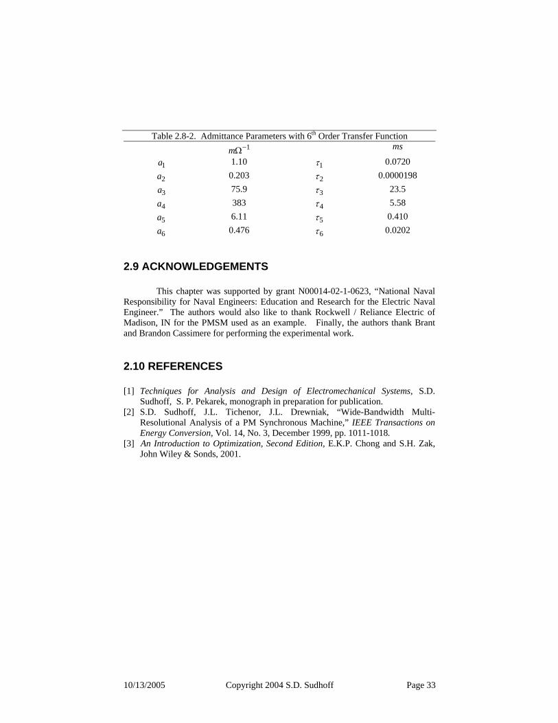
Table 2.8-2. Admittance Parameters with 6th Order Transfer Function
1−Ωm ms
1a 1.10 1τ 0.0720
2a 0.203 2τ 0.0000198
3a 75.9 3τ 23.5
4a 383 4τ 5.58
5a 6.11 5τ 0.410
6a 0.476 6τ 0.0202
2.9 ACKNOWLEDGEMENTS This chapter was supported by grant N00014-02-1-0623, “National Naval Responsibility for Naval Engineers: Education and Research for the Electric Naval Engineer.” The authors would also like to thank Rockwell / Reliance Electric of Madison, IN for the PMSM used as an example. Finally, the authors thank Brant and Brandon Cassimere for performing the experimental work.
2.10 REFERENCES [1] Techniques for Analysis and Design of Electromechanical Systems, S.D.
Sudhoff, S. P. Pekarek, monograph in preparation for publication. [2] S.D. Sudhoff, J.L. Tichenor, J.L. Drewniak, “Wide-Bandwidth Multi-
Resolutional Analysis of a PM Synchronous Machine,” IEEE Transactions on Energy Conversion, Vol. 14, No. 3, December 1999, pp. 1011-1018.
[3] An Introduction to Optimization, Second Edition, E.K.P. Chong and S.H. Zak, John Wiley & Sonds, 2001.


