
ECONOMICS
ENERGY INTENSITY AND ITS DETERMINANTS IN CHINA’S REGIONAL ECONOMIES
by
Yanrui Wu
Business School University of Western Australia
DISCUSSION PAPER 11.25

ENERGY INTENSITY AND ITS DETERMINANTS IN CHINA’S
REGIONAL ECONOMIES*
Yanrui Wu
Economics Program (M251) UWA Business School
University of Western Australia WA 6009, Australia
[email protected] 618 6488 3964 (tel) 618 6488 1016 (fax)
Forthcoming in Energy Policy
DISCUSSION PAPER 11.25
* Work on this paper was supported by an ARC Discovery Project grant (DP1092913). I thank James Cheong, Dahai Fu and Nickolas Sin for their excellent research assistance, and Professor Bin Wang of Jinan University for assistance with data collection. I also acknowledge the participants of ACESA2010 (La Trobe University, 2010) and the 12th EAEA convention (Ewha Womans University, 2010), Enjiang Cheng, Chunbo Ma, and Rachel C. Reyes for helpful comments and suggestions.
ABSTRACT
This paper contributes to the existing literature as well as policy debates by examining
energy intensity and its determinants in China’s regional economies. The analysis is
based on a comprehensive database of China’s regional energy balance constructed
for this project. Through its focus on regional China, this study extends the existing
literature which mainly covers nationwide studies. It is found in this paper that energy
intensity declined substantially in China. The main contributing factor is the
improvement in energy efficiency. Changes in the economic structure have so far
affected energy intensity modestly. Thus there is considerable scope to reduce energy
intensity through the structural transformation of the Chinese economy in the future.
Key words Energy intensity, energy efficiency, structural change and China
JEL codes Q43, R11 and Q48

1
1. Introduction
Over the past three decades the Chinese economy has indeed achieved impressively
high growth. This growth is however associated with deteriorating environmental
conditions in the country (World Bank 2001, Wu 2010). With increasing
environmental awareness in the society and demand for better quality of life by
ordinary citizens, Chinese policy makers are under tremendous pressure to rechart the
country’s course of growth in the coming decades. A key issue of concern is related to
energy consumption which is the main source of pollutants in the air, soil and water.
China is now the world’s largest energy consumer as well as CO2 emitter. The
country’s energy consumption pattern will have important implications for the global
environment.
So far the literature has focused on forecasting future energy consumption in China
particularly at the aggregate level (Crompton and Wu 2003, IEA 2009). There are a
few papers which investigated China’s energy intensity (defined as the ratio of energy
consumption over output such as GDP). As shown in Table 1, these studies can be
broadly divided into several groups, namely, national, regional, sectoral and other
studies. First, Garbaccio et al. (1999) and Ma and Stern (2008) adopted different
decomposition methods to examine energy intensity at the national level. Second,
Huang (1993), Sinton and Levine (1994) and Zhang (2003) represented earlier studies
of energy intensity in China’s industrial sector in the 1980s and 1990s. Recently Liao
et al. (2007) and Zhao et al. (2010) extended earlier studies to sub-sectors at the two-
digit level. All sectoral studies followed the decomposition method. Zheng et al.
(2011) is an exception which applied regression analysis to investigate the impact of
exports on energy intensity in 20 sub-sectors during 1999-2007.

2
Table 1 Major Studies of China’s Energy Intensity __________________________________________________________________ Authors Data Method National/aggregate level Garbaccio et al. (1999) 1987 & 1992 I-O tables/index method Ma and Stern (2008) 1980-2003 LMDI Sectoral level Huang (1993) 1980-88 Divisia index/Industry Sinton and Levine (1994) 1980s Laspeyres index/Industry Zhang (2003) 1990s IDA/29 sub-sectors Liao et al. (2007) 1997-2006 IDA/36 sub-sectors Zhao et al. (2010) 1998-2006 LMDI/15 sub-sectors Zheng et al. (2011) 1999-2007 Regressions/20 sub-sectors (exports) Regional Qi and Luo (2007), 1995-2002 Regressions Li and Wang (2008) 1995-2005 LMDI Ma et al. (2009) 1995-2004 Cost functions Wang and Zhong (2009). 1995-2006 Regressions Yuxiang and Chen 2010 1996-2006 Regressions/government spending Other studies Fisher-Vanden et al. (2004) 1997-99 Divisia/regressions (firm level) Golley (2008) 2005 Energy requirement (household level) Chai et al. (2009) 4 years I-O tables/30 sub-sectors (1992-2004) __________________________________________________________________ Source: Author’s own compilation. Note: I-O tables: Input-output tables. LMDI: Logarithmic mean Divisia index. IDA: Index decomposition analysis.
Third, several recent papers employed provincial (regional) data and regression
techniques to examine China’s energy intensity. For example, Qi and Luo (2007)
investigated the relationship between energy intensity and economic growth, Wang
and Zhong (2009) explored the effect of regional resource endowment on energy
intensity, and Yuxiang and Chen (2010) examined the impact of government
expenditure on energy intensity. Furthermore, Ma et al. (2009) investigated the
substitutability between fuels and between energy and factor inputs (capital and
labour) and Li and Wang (2008) adopted the popular logarithmic mean Divisia index

3
(LMDI) approach to understand energy intensity changes across the regions. Finally,
several papers are differentiated from the national, sectoral and regional studies just
reviewed. Fisher-Vanden et al. (2004) is the first paper with a focus on energy
intensity at the firm-level (involving data of 2500 firms and three years 1997-1999).
Golley et al. (2008) presented a detailed study of energy requirement and CO2
emissions at household level in urban China. Chai et al. (2009) employed a
decomposition method involving the input-output table to explore how various factors
affect energy intensity in China.
The present study extends the existing literature in two ways. The analysis is for the
first time based on sectoral energy consumption data in the Chinese regions. In
addition, it applies regression analyses to examine the determinants of energy
intensity and its components at the regional level. It is found in this study that there is
considerable regional disparity in energy intensity as well as its trend of movement
over time. It is also shown in the empirical analysis that changes in regional energy
intensity are mainly affected by energy efficiency changes with hardly any impact
from economic structural transformation in the regions. This finding implies the need
for urgent policy actions in order to reduce energy intensity through structural
changes in China’s regional economies in the coming decades. Other factors which
are important for the reduction in energy intensity include energy prices and adoption
of new technologies in regional economies.
The rest of the paper begins with Section 2 where energy intensity at the national
level is briefly discussed. Section 3 then presents a preliminary analysis of energy
intensity in the regions. Subsequently, regression analysis in Section 4 is employed to

4
investigate the determinants of regional intensity variations. This is followed by
further discussions of selected issues in Section 5. The concluding remarks are
presented in Section 6.
2. Energy Intensity in China
During the period of 1953-2009 the movement of China’s energy intensity basically
followed an inverted U-shaped curve though total energy consumption increased
steadily (Figure 1). Before the country’s economic reform program was introduced in
1978, energy intensity fluctuated considerably and its overall trend of changes was
upward. It peaked twice in 1960 and 1977, respectively. This course of changes is
consistent with the pattern of economic growth before 1978. During that period, the
Chinese economy experienced a few ups and downs due to political chaos and poor
economic policies. However, during the post-reform decades (1978-2009), energy
intensity basically followed a declining trend though there were temporary disruptions
in several years, namely, in 1989 and during 2003-2005 when energy intensity was
recorded with a minor increase. Thus the “dematerialization” phenomenon was also
observed in China as income increases over time (Bernardini and Galli 1993). In
international perspectives, China’s energy intensity is converging rapidly with major
energy consumers in the world (Figure 2). Especially, China seems to follow the
similar paths undergone by Japan and South Korea. If the overall trend is maintained,
China could even do better than the major economies in terms of energy intensity
reduction in the future (refer to the solid line in Figure 2).

5
0
100
200
300
400
500
600
1953
1955
1957
1959
1961
1963
1965
1967
1969
1971
1973
1975
1977
1979
1981
1983
1985
1987
1989
1991
1993
1995
1997
1999
2001
2003
2005
2007
2009
Year
Inte
nsity
0
500
1000
1500
2000
2500
3000
3500
Con
sum
ptio
n
Energy intensity
Energy consumption
Note: Energy intensity is expressed in kilograms coal equivalent per 1000 yuan in 2000 prices and energy consumption in million tons (MTs) coal equivalent. Sources: NBS (various issues, 2009 and 2010). Figure 1 China’s Energy intensity 1953-2009
0
200
400
600
800
1000
1200
0 5000 10000 15000 20000 25000 30000 35000 40000
ppp$
Kg/
ppp$
1000
India
China
JapanSouth Korea
Germany
USA
Note: The unit of energy intensity is kilogram of oil equivalent per ppp$1000 in 2005 constant prices. The data are based on statistics during 1980-2007 for each country. Source: Author’s own calculation using data from the World Bank (2010). Figure 2 Energy intensity and Economic Development

6
To gain a better understanding of the trend in China’s energy intensity, the following
decomposition approach is considered
/ it itt t t i i it it i it
it t
C YI C Y E S I
Y Y (1)
where It, Ct and Yt represent energy intensity, energy consumption and GDP. The
economy is divided into three sectors, namely, the primary, manufacturing and service
sectors.1 Energy is consumed in the three sectors and for residential purposes (i=1, 2,
3 and 4). Eit and Sit are employed to measure energy use efficiency and shares of
economic activities (or value-added over GDP in the sectors). For the residential
sector, value-added is replaced by the value of household consumption.
Equation (1) implies that energy intensity is linked with energy efficiency and sectoral
output shares, respectively. This is the so-called index decomposition analysis (IDA)
technique proposed and widely used in the literature. Empirically authors have
adopted either the Divisia index or the Laspeyres index method.2 Several comparative
studies however show that the log mean Divisia index (LMDI) method is preferred to
other index approaches (Greening et al. 1997, Ang 2004). Following the IDA
approach, changes in energy intensity (ΔIt) can be decomposed into two components
which may be called the efficiency and structural change components, respectively.
On the one hand, the efficiency component (ΔEt) refers to changes in energy intensity
which are associated with changes in energy use efficiency. On the other hand, the
1 Ma and Stern (2008) presented a more disaggregate decomposition analysis at the national level for the period of 1994-2003. 2 Ang and Zhang (2000) presented a comprehensive review of the literature, particularly various IDA methods.
7
structural change component (ΔSt) captures the contribution of economic structural
changes to energy intensity variation. Symbolically, the additive version can be
presented as3
t t tI E S (2)
where
1t t tI I I (3)
, 1
, 1 , 1
ln( )ln ln
it i t itt i
it i t i t
I I EE
I I E
(4)
, 1
, 1 , 1
ln( )ln ln
it i t itt i
it i t i t
I I SS
I I S
(5)
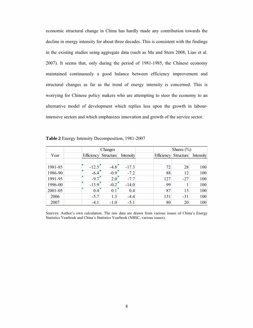
Following the system of Equations (1) to (5), the year-to-year variations in energy
intensity together with the contributions of the efficiency and structural change
components are estimated. The 5-year span mean values are presented in Table 2. The
5-year spans correspond to China’s Five Year Plan cycles. According to this table,
China’s energy intensity declined in most periods during 1981-2007 with the
exception of the years of 2001-2005.4 The main contributing factor for the decline in
energy intensity is efficiency improvement. With the exception of the period of 1981-
1985, structural change has only made marginal contributions to the decline in energy
intensity. This phenomenon is clearly demonstrated in the three indexes reflecting the
accumulated changes in energy intensity, the efficiency and structural change
components over time (see Figure 3). While energy intensity fell substantially
between 1980 and 2007, the curve of the structural change index is almost flat. Thus
3 Technical details are available in Ang (2005). 4 For detailed exploration of the fall and rise of energy intensity in China, the redears may refer to Liao et al. (2007) and Zhao et al. (2010).
8
economic structural change in China has hardly made any contribution towards the
decline in energy intensity for about three decades. This is consistent with the findings
in the existing studies using aggregate data (such as Ma and Stern 2008, Liao et al.
2007). It seems that, only during the period of 1981-1985, the Chinese economy
maintained continuously a good balance between efficiency improvement and
structural changes as far as the trend of energy intensity is concerned. This is
worrying for Chinese policy makers who are attempting to steer the economy to an
alternative model of development which replies less upon the growth in labour-
intensive sectors and which emphasizes innovation and growth of the service sector.
Table 2 Energy Intensity Decomposition, 1981-2007
Changes Shares (%)Year Efficiency Structure Intensity Efficiency Structure Intensity
1981-85 -12.5 -4.8 -17.3 72 28 1001986-90 -6.4 -0.9 -7.2 88 12 1001991-95 -9.7 2.0 -7.7 127 -27 1001996-00 -13.9 -0.2 -14.0 99 1 1002001-05 0.4 0.1 0.4 87 13 100
2006 -5.7 1.3 -4.4 131 -31 1002007 -4.1 -1.0 -5.1 80 20 100
Sources: Author’s own calculation. The raw data are drawn from various issues of China’s Energy Statistics Yearbook and China’s Statistics Yearbook (NBSC, various issues).

9
0.0
0.2
0.4
0.6
0.8
1.0
1.2
1980
1981
1982
1983
1984
1985
1986
1987
1988
1989
1990
1991
1992
1993
1994
1995
1996
1997
1998
1999
2000
2001
2002
2003
2004
2005
2006
2007
Inde
xes
Year
Intensity
Efficiency
Economic structure
Sources: Author’s own calculations. The raw data are drawn from various issues of China’s Energy Statistics Yearbook and China’s Statistics Yearbook (NBSC, various issues). Figure 3 Intensity, Efficiency and Structural Indexes, 1980-2007
3. Energy Intensity in the Regions
There are few studies focusing on energy intensity in China’s regional economies
largely due to the scarcity of data. Hu and Wang (2006) and Dan (2007) are two
exceptions. Hu and Wang employed the data envelopment analysis (DEA) approach
to compare the potential energy consumption with actual energy use in the regions.
They divided China geographically into three regions and found that the central
region had the lowest average energy efficiency during the period 1995-2002. Dan
examined the so-called regional energy efficiency which is defined as the ratio of
gross regional product (GRP) per unit of energy use (this is contrary to the
conventional energy intensity concept). Dan showed the existence of substantial
variations in regional energy efficiency and argued that the coastal regions on average
performed better than the rest of the country during 1990-2004. None of them
however explored energy intensity at the sector level among the regions. To prepare
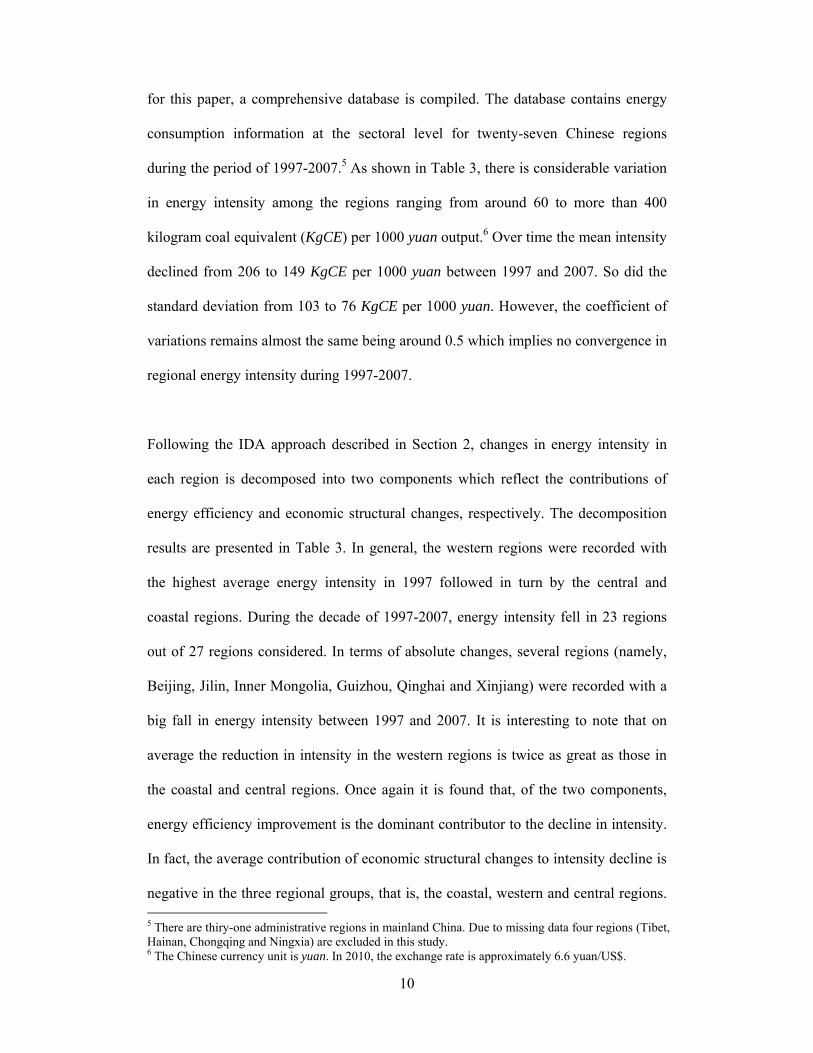
10
for this paper, a comprehensive database is compiled. The database contains energy
consumption information at the sectoral level for twenty-seven Chinese regions
during the period of 1997-2007.5 As shown in Table 3, there is considerable variation
in energy intensity among the regions ranging from around 60 to more than 400
kilogram coal equivalent (KgCE) per 1000 yuan output.6 Over time the mean intensity
declined from 206 to 149 KgCE per 1000 yuan between 1997 and 2007. So did the
standard deviation from 103 to 76 KgCE per 1000 yuan. However, the coefficient of
variations remains almost the same being around 0.5 which implies no convergence in
regional energy intensity during 1997-2007.
Following the IDA approach described in Section 2, changes in energy intensity in
each region is decomposed into two components which reflect the contributions of
energy efficiency and economic structural changes, respectively. The decomposition
results are presented in Table 3. In general, the western regions were recorded with
the highest average energy intensity in 1997 followed in turn by the central and
coastal regions. During the decade of 1997-2007, energy intensity fell in 23 regions
out of 27 regions considered. In terms of absolute changes, several regions (namely,
Beijing, Jilin, Inner Mongolia, Guizhou, Qinghai and Xinjiang) were recorded with a
big fall in energy intensity between 1997 and 2007. It is interesting to note that on
average the reduction in intensity in the western regions is twice as great as those in
the coastal and central regions. Once again it is found that, of the two components,
energy efficiency improvement is the dominant contributor to the decline in intensity.
In fact, the average contribution of economic structural changes to intensity decline is
negative in the three regional groups, that is, the coastal, western and central regions. 5 There are thiry-one administrative regions in mainland China. Due to missing data four regions (Tibet, Hainan, Chongqing and Ningxia) are excluded in this study. 6 The Chinese currency unit is yuan. In 2010, the exchange rate is approximately 6.6 yuan/US$.

11
These regional differences call for further investigation into the determinants of the
variation in regional energy intensity.
Table 3 Energy Intensity and Changes between 1997 and 2007
Regions Energy intensity Absolute Component changes1997 2007 changes Efficiency Structure
Beijing 206.4 83.6 -122.7 -97.3 -25.4Tianjin 187.1 94.8 -92.4 -96.6 4.3Hebei 246.8 225.5 -21.3 -31.1 9.9Liaoning 310.0 284.4 -25.6 -32.7 7.1Shanghai 170.6 82.9 -87.8 -83.2 -4.6Jiangsu 104.5 81.3 -23.2 -28.9 5.6Zhejiang 78.9 60.1 -18.8 -17.1 -1.7Fujian 59.7 80.9 21.3 15.2 6.1Shandong 98.2 98.6 0.3 -9.8 10.1Guangdong 81.3 62.0 -19.3 -22.3 3.1Coastal mean 154.4 115.4 -39.0 -40.4 1.4
Shanxi 404.5 391.5 -12.9 -36.9 24.0Jilin 328.5 167.8 -160.7 -183.8 23.1Heilongjiang 186.9 112.3 -74.6 -67.5 -7.2Anhui 164.1 109.5 -54.6 -39.7 -14.9Jiangxi 141.6 181.4 39.9 13.2 26.6Henan 161.5 132.6 -28.9 -45.4 16.5Hubei 170.2 124.4 -45.8 -34.7 -11.1Hunan 134.9 133.9 -1.0 -4.6 3.6Central mean 211.5 169.2 -42.3 -49.9 7.6
InnerMongolia 435.3 224.8 -210.5 -261.5 51.1Guangxi 111.4 140.6 29.2 22.9 6.3Sichuan 154.6 90.0 -64.5 -66.5 1.9Guizhou 384.5 226.5 -157.9 -175.6 17.6Yunnan 192.5 187.9 -4.6 9.8 -14.4Shaanxi 196.0 102.1 -93.9 -109.6 15.7Gansu 271.5 184.4 -87.1 -91.3 4.2Qinghai 307.3 182.3 -125.0 -180.1 55.0Xinjiang 284.2 174.9 -109.3 -139.4 30.1Western mean 259.7 168.2 -91.5 -110.1 18.6
Sources: Author’s own calculation. The raw data are drawn from various issues of China’s Energy Statistics Yearbook and China’s Statistics Yearbook (NBSC, Various issues).

12
4. Determinants of Regional Energy Intensity
To understand regional variation in energy intensity and its determinants, three
regional indices similar to those in Figure 3 are computed using the decomposition
results from Section 3. The indices relative to the initial year (1997) capture the trends
in energy intensity change and its two components over time. To examine the
determinants of regional variation, the indices reflecting the two components, namely,
the energy efficiency (EEit) component and structural change (SCit) component, are
regressed against a set of region-specific covariates or explanatory variables (Xit).
Symbolically,
0it j j ijt itY X (6)
where Yit represents either the efficiency index (EEit) or the structural change index
(SCit) for region i and at year t. The covariates (Xijt) are selected to capture specific
characteristics of regional economies and detailed as follows.
An income (Income) variable is included to reflect the level of economic development
in the regions. It is measured by per capita gross regional product (GRP) which is
expressed in 2000 constant prices. It is argued that energy efficiency generally
improves as an economy develops.7 In accordance with this argument, the coefficient
of the Income variable is expected to be negative.
7 “A Better World for All”, a report of the Progress towards the International Development Goals project jointly conducted by the IMF, OECD, United Nations and World Bank, 2000 (http://www.paris21.org/sites/default/files/bwa_e.pdf).

13
A price (Price) variable is considered to evaluate the impact of fuel prices on energy
intensity. As China’s fuel price data are not available, the fuel price index for each
region is employed as a proxy of fuel prices. It is also expressed in terms of 2000
constant prices. In general, an increase in energy prices raises the cost of production.
Producers may respond by improving energy efficiency. Thus the coefficient of the
Price variable is expected to be negative.
Other variables considered include the capital-labour ratio (Klratio) and the growth
rate of capital stock (Krate). On the one hand, it is argued that energy and technology
or capital may be substitutes (Thompson and Taylor 1995, Metcalf 2008). The capital-
labour ratio here is employed as a proxy of the level of technology involved. Thus the
capital-labour ratio (Klratio) variable may be negatively related to energy intensity.
That is, energy intensity is expected to decline as production technology improves. On
the other hand, the growth of capital stock may to some extent reflect the speed of old
machines and structures being replaced and is hence introduced as a measure of the
vintage of capital. New capital may be endowed with energy-saving technology and is
thus more energy efficient. Therefore, the coefficient of the Klratio variable is
expected to be negative. A time trend (Time) is also included in the model to capture
the trend of change over time and is expected to have a negative coefficient.
The baseline model estimated is a fixed effect log-log model. The estimation results
are presented in Table 4. The lagged values of some explanatory variables are
employed to avoid the problem of simultaneity. Model 1 is the simple version of
Equation (6). The estimated coefficients of the Income, Price and Time trend variables
have the expected sign and are statistically significant. The coefficients of the capital-

14
labour ratio (Klratio) and capital stock growth (Krate) variables have the wrong sign.
To consider the possibility of non-linearity, the squared terms of those variables are
added to the model. The estimation results of the optional model (Model 2 in Table 4)
confirm the existence of nonlinear relationship as the estimated coefficients of the
squared terms are statistically significant. The values of the adjusted R2 also indicate
that Model 2 is preferred to Model 1. The F test statistic also shows that the fixed
effects are statistically significant.8
8 The fixed effect model is also tested against the random effect model. However, for both Models 1 and 2, the Hausman test statistics are collapsed. The estimation results of the random effect model (not reported) do show insignificant coefficients for several explanatory variables.
15
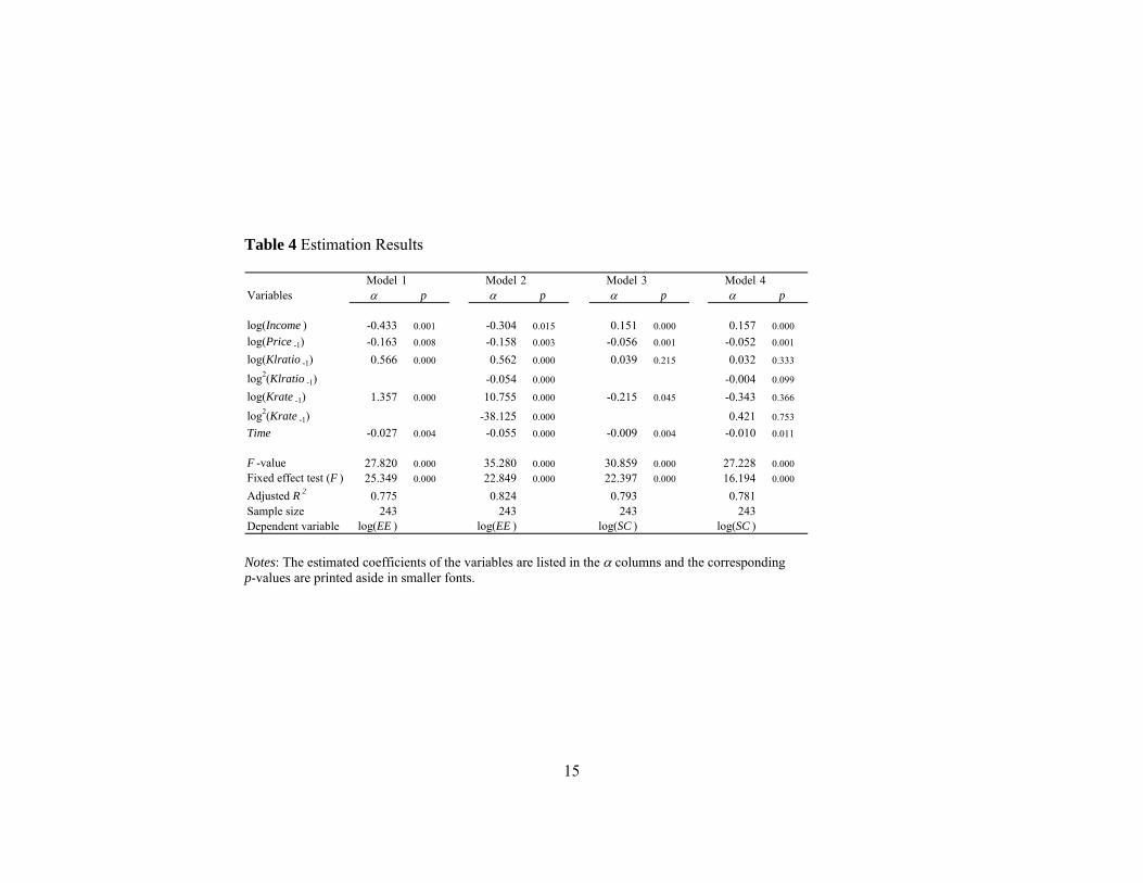
Table 4 Estimation Results
Model 1 Model 2 Model 3 Model 4Variables p p p p
log(Income ) -0.433 0.001 -0.304 0.015 0.151 0.000 0.157 0.000
log(Price -1) -0.163 0.008 -0.158 0.003 -0.056 0.001 -0.052 0.001
log(Klratio -1) 0.566 0.000 0.562 0.000 0.039 0.215 0.032 0.333
log2(Klratio -1) -0.054 0.000 -0.004 0.099
log(Krate -1) 1.357 0.000 10.755 0.000 -0.215 0.045 -0.343 0.366
log2(Krate -1) -38.125 0.000 0.421 0.753
Time -0.027 0.004 -0.055 0.000 -0.009 0.004 -0.010 0.011
F -value 27.820 0.000 35.280 0.000 30.859 0.000 27.228 0.000
Fixed effect test (F ) 25.349 0.000 22.849 0.000 22.397 0.000 16.194 0.000
Adjusted R 2 0.775 0.824 0.793 0.781Sample size 243 243 243 243Dependent variable log(EE ) log(EE ) log(SC ) log(SC )
Notes: The estimated coefficients of the variables are listed in the columns and the corresponding p-values are printed aside in smaller fonts.

16
Several conclusions can be drawn from the estimation results of the fixed effect
model. First, energy efficiency improves as income per capita increases among the
Chinese regions. Thus, as the regions become more developed, energy use becomes
more efficient and hence energy intensity falls. Second, energy price movement is
negatively related to energy efficiency. That is, the efficiency component index tends
to decline (a positive contribution to intensity decline) as prices increase. The average
price elasticity is estimated to be -0.158. This finding is consistent with the
observation by Ma et al. (2009) who showed that energy intensity declined by
approximately 20% during 2000-2004 due to increasing energy prices. Third, it is
confirmed that the efficiency index and capital-labour ratio variable have an inverted
U-shaped relationship. However the estimated average turning point is far greater than
the actual capital-labour ratios for the Chinese regions. Thus at the current level of
development, it seems that there is no substitution effect between capital and energy
in China’s regional economies. Fourth, the non-linear relationship between the
efficiency component index and growth in capital stock or vintage of capital variable
shows that technology embodied in new capital may help improve efficiency after
growth reaches certain level. The estimated turning point is an average rate of growth
of 15.1 per cent. In 2007, seven out of the 27 regions included in the sample surpassed
the turning point rate of growth. Thus those regions may have benefited from the
speedy replacement of old equipment and structures. Finally, the estimation results
show that the efficiency component index tends to fall over time. This is consistent
with the positive contribution of the efficiency component to the decline in energy
intensity observed in the preceding section.

17
For the purpose of comparison, the structural change component index is also
regressed against the same set of covariates. The regression results are presented in
Table 4 (Models 3 and 4). Apparently Model 3 without the squared terms is preferred
to Model 4 in which the two estimated coefficients of the squared terms are
statistically insignificant. The estimated coefficients in Model 3 have the expected
sign with two exceptions. First, the estimated coefficient of the Income variable in
Model 3 is positive and statistically significant. Thus as regional economies grow,
structural change has not led to the reduction in energy intensity. On the contrary, it
might play the role in raising energy intensity in some regions. This is consistent with
the findings from the preliminary analysis. Second, Model 3 also shows a positive
relationship between the structural change component index and capital-labour ratio
but this relation is statistically insignificant.
5. Further Considerations
The analyses in the preceding section are likely affected by several factors. The first
factor is the possible existence of unit roots in the variables included in the models.
The results of five tests for unit roots are mixed as some tests are statistically
significant and others are not (see Table 5). To explore this issue further, the popular
generalized method of moments (GMM) is employed to re-estimate the models. In
addition, it is assumed that the use of GMM may also correct potential problems with
multicollinearity, heteroscedasticity and autocorrelation of unknown forms in the
models. Finally, there may be potential problems with endogeneity in the models
reported in Table 4. This is another reason to adopt the GMM approach.

18
Table 5 Unit Root Test Results
Variables LLC Breitung IPS ADF PP
log(EE ) -7.104 -0.687 -0.225 63.927 81.9800.000 0.246 0.411 0.167 0.008
log(SC ) -5.739 2.293 0.759 40.518 60.0640.000 0.989 0.776 0.913 0.266
log(Income ) -20.178 0.585 -4.085 162.082 44.2090.000 0.721 0.000 0.000 0.827
log(Price ) -16.500 0.980 -3.366 142.243 180.8690.000 0.837 0.000 0.000 0.000
log(Klratio ) -16.108 -2.463 -1.941 111.487 62.1140.000 0.007 0.026 0.000 0.210
log2(Klratio ) -18.182 1.104 -4.296 168.922 103.4560.000 0.865 0.000 0.000 0.000
log(Krate ) -5.562 1.040 0.655 47.076 132.4450.000 0.851 0.744 0.736 0.000
log2(Krate ) -2.601 7.864 1.256 38.012 110.4870.005 1.000 0.896 0.951 0.000
Notes: The p-value is presented underneath each statistic. LLC: Levin, Lin and Chu t test; Breitung: Breitung t statistic; IPS: Im, Pesaran and Shin Wald statistic;
ADF: ADF Fisher 2 test; and
PP: PP Fisher 2 test.
Source: Author’s own calculation.
The estimation results are illustrated in Table 6 (Models 5 and 6) are estimated using
the efficiency component index as the dependent variable. A major issue with the
GMM approach is the choice of instrumental variables (IVs) which can lead to over-
identification of the model. To deal with this problem, the number of IVs is controlled
and the Sargan test is conducted. The IVs used in each model are described in the
notes to Table 6. Both models (5 and 6) passed the Sargan test for over-identification.

19
To tackle the possible presence of serial correlation, the estimation method built-in in
Eviews 7 is employed here.9 It is assumed that the errors for a cross-section are
heteroscedastic and serially correlated. Under this assumption, the coefficient
covariance is calculated and hence the corrected standard errors of the estimated
coefficients are reported. The results from the static GMM estimation (Model 5) are
generally consistent with those from Model 2 in Table 4.
Table 6 GMM Estimation Results
Model 5 Model 6 Model 7 Model 8Variables p p p p
log(EE -1 ) 0.310 0.000
log(SC -1 ) 0.579 0.000
log(Income ) -0.284 0.000 0.147 0.000 -0.010 0.961 0.057 0.000
log(Price -1 ) -0.268 0.000 -0.011 0.059 -0.166 0.045 -0.009 0.415
log(Klratio -1 ) 0.351 0.000 0.015 0.001 0.422 0.000 0.018 0.061
log2(Klratio -1 ) -0.047 0.000 -0.042 0.001
log(Krate -1 ) 2.857 0.004 0.226 0.000 2.795 0.049 0.165 0.000
log2(Krate -1 ) -8.040 0.010 -10.189 0.023
Time -0.022 0.068 -0.010 0.000 -0.060 0.043 -0.004 0.046
Sargan statistic 20.340 0.729 26.527 0.489 12.613 0.943 19.352 0.681
Sample size 216 216 216 216Dependent variable log(EE ) log(SC ) log(EE ) log(SC )
Notes: The estimated coefficients of the variables are listed in the columns and the corresponding p-values are printed aside in smaller font. The IVs used in each model include all independent variables and the dependent variable with lags (from 3 to 5 using the @DYN (log (EE),-3,-5) command in model 5, @DYN (log (SC),-3,-6) in model 6, @DYN (log (EE),-4,-6) in model 7 and @DYN (log (SC),-4,-7) in model 8. The Time trend variable is untransformed using the @LEV(Time) command. The standard errors of the estimated coefficients are corrected for serial correlation. The second factor is associated with the inclusion of lagged values. In the preceding
sections, while one-period lagged values are used to avoid the potential problem of
simultaneity, the lag period could last well beyond one year. For example, a change in
energy prices or capital-labour ratios may affect energy intensity (as well as its
9 In Eviews, it is called the “white period method” (Arellano 1987, White 1980).

20
components) over a few years. To deal with this problem, a partial adjustment model
is considered.10 This model can be expressed as follows
*0it j ijt itY X (7)
*, 1 , 1( )it i t it i tY Y Y Y (8)
where *itY is the desired efficiency (component) in the ith region and tth year and is
the coefficient of adjustment. Combining Equations (7) and (8) yields
0 , 1(1 )it j j ijt i t itY X Y (9)
where j is the short-run impact of a change in X on Y and j gives the long-run
impacts. Thus the model becomes a dynamic panel data model and can also be
estimated using GMM which is now called the dynamic GMM (vs static GMM). The
estimation results are reported in Table 6 (Models 7 and 8). For the dynamic GMM
estimation, the estimated coefficients of all variables but Income are statistically
significant. The estimated adjustment coefficient is 0.69. 11 Thus the elasticity of
‘efficiency’ with respect to price is -0.166 in the short run (Model 7) and -.241 in the
long run.12 These numbers imply that energy price may play a more important role in
reducing intensity in the long run.
10 Metcalf (2008) employed the same adjustment process to examine energy intensity and its determinants at the state level in the US. 11 The adjustment coefficient =0.69 is derived using the coefficient (1-) of log(EE-1) in Model 7. 12 The long run price elasticity (-0.241) is the short run elasticity (-0.166) divided by the coefficient of adjustment (0.69).
21
For the structure models (Models 6 and 8), the results from both static and dynamic
GMM estimations are generally consistent with those from the fixed effect estimation,
that is, Model 3 in Table 4. Energy price is found to have a negative impact on the
structural change component (and hence a positive effect on the reduction of energy
intensity) but this effect is not statistically significant. The coefficients of other
variables (Income, KLratio and Krate) are also estimated with the wrong sign which is
consistent with the decomposition result that structural change component has made
little contribution towards the fall in energy intensity among the Chinese regions
during 1998-2007.
The last point is however subjected to serious qualification. It should be emphasized
that, due to data constraints, the analyses in this paper are highly aggregate and only
cover three sectors, agriculture, manufacturing and services. During the sampled
period of 1998-2007, structural change might take place within the manufacturing
sector in each region. This change cannot be captured in the empirical exercises here
and may be partly responsible for the decline in energy intensity and hence efficiency
improvement. To shed some light on this issue, Table 7 presents the output shares and
energy intensity in China’s twenty-eight manufacturing sectors in 1998 and 2007,
respectively. Within a decade, energy intensity in the manufacturing sector declined
by about two-thirds. If we follow the index decomposition analysis proposed in
section 2, we can show that the decline (-34.5) is purely due to energy efficiency
improvement (-37.8) with structural changes having a negative contribution (3.3).
This is confirmed in Table 7 which demonstrates that the high energy-intensive
sectors (the top 10) all experienced a decline in energy intensity while the changes in
output shares are mixed. This is of course based on economy-wide statistics. There

22
may be regional variations which call for further investigation when information
becomes available.
Table 7 China’s Energy Intensity and Output Shares by Sector
Sectors Energy intensity Value-added shares1998 2007 Changes 1998 2007 Changes
Smelting and Pressing of Ferrous Metals 184.8 53.0 -131.7 6.5 9.7 3.1 Raw Chemical Materials and Chemical Products 142.3 37.1 -105.2 7.4 7.9 0.5 Petroleum Processing and Coking 139.8 42.5 -97.2 3.5 3.3 -0.2 Nonmetal Mineral Products 135.5 42.0 -93.5 6.1 5.2 -0.8 Smelting and Pressing of Nonferrous Metals 99.1 23.9 -75.2 2.2 4.8 2.6 Chemical Fiber 77.7 19.2 -58.5 1.2 0.9 -0.4 Papermaking and Paper Products 60.9 19.2 -41.8 2.1 1.9 -0.2 Rubber Products 30.7 13.1 -17.6 1.4 1.0 -0.3 Textile Industry 30.3 12.6 -17.6 6.8 5.3 -1.5 Food Production 30.2 7.1 -23.1 2.2 2.0 -0.2 Timber Processing, Palm Fiber and Straw Products etc 30.1 8.0 -22.1 0.8 1.1 0.4 Food Processing 26.9 5.0 -21.9 4.5 5.0 0.5 Ordinary Machinery 22.4 5.1 -17.3 4.6 5.5 0.9 Furniture Manufacturing 21.1 2.3 -18.8 0.5 0.7 0.2 Metal Products 20.7 9.4 -11.3 3.4 3.2 -0.1 Plastic Products 19.3 7.6 -11.7 2.4 2.3 -0.1 Medical and Pharmaceutical Products 19.3 5.2 -14.1 2.9 2.5 -0.4 Equipment for Special Purposes 18.3 4.7 -13.6 3.2 3.3 0.1 Beverage Production 14.2 5.2 -9.0 3.6 2.0 -1.6 Transportation Equipment 14.1 3.4 -10.7 7.2 7.5 0.3 Printing and Record Medium Reproduction 9.6 4.7 -5.0 1.2 0.7 -0.5 Electric Equipment and Machinery 7.4 2.5 -4.8 5.9 6.5 0.7 Leather, Furs, Down and Related Products 5.8 2.5 -3.3 1.8 1.6 -0.2 Garments and Other Fiber Products 5.8 3.0 -2.8 3.2 2.4 -0.8 Cultural, Educational and Sports Articles 5.6 3.7 -1.9 0.9 0.6 -0.3 Instruments, Meters, Cultural and Office Machinery 4.9 2.2 -2.7 1.1 1.3 0.1 Electronic and Telecommunications Equipment 4.4 2.5 -1.9 7.5 8.5 1.1 Tobacco Processing 2.9 0.8 -2.1 5.9 3.1 -2.8
Total 51.1 16.7 -34.5
Note: Value-added shares are percentage shares. Energy intensity is expressed in kilograms coal equivalent per 1000 yuan.
6. Conclusion
To sum up, it is shown in this study that the overall trend of the movement of China’s
energy intensity in the past decades has been declining. The main driving force for the
decline is due to the improvement in energy efficiency while the impact of structural
changes in the economy is very limited. There is however substantial variation in

23
energy intensity and its trend of changes in Chinese regional economies. In absolute
terms, among the 27 regions considered, the highest energy intensity is six or seven
times as high as the lowest one. During the period of 1997-2007, the average energy
intensity declined. In conformity with the national trend, the decline is mainly due to
efficiency improvement with little contribution from economic structural changes. But
the changes in energy intensity are very uneven. Some regions experienced a
substantial decrease in energy intensity while others were recorded with a modest
increase during 1997-2007. Furthermore, it seems that there was no evidence of
convergence in regional energy intensity in the past decade.
To understand regional variation in energy intensity, the intensity component indices,
namely the efficiency and structural change indices, are regressed against several
region-specific covariates. It is found that energy intensity declines as income rises
among the regions. Thus China’s regional economies generally follow the same
dematerialization process as most developed economies have undergone. However
“dematerialization” at the current stage of development in China is not due to shifts in
manufacturing activities rather it is mainly because of energy efficiency improvement
within the sectors. It can be anticipated that China’s energy intensity can be reduced
further when structural changes become the main driver for dematerialization. For this
reason, an optimistic view is that in terms of energy intensity China could even
perform better than its East Asian counterparts, Japan and South Korea. It is also
found in this study that energy intensity is responsive to energy prices in both the
short run and the long run. Thus getting energy prices right is important for reducing
energy consumption and hence emissions in China.
24
Finally, there is evidence of the existence of nonlinear relationship between energy
intensity and capital-labour ratios. However, it seems that all Chinese regions are still
on the left hand side of the inverted U-shaped curve. Hence the sample considered
does not support the argument that capital and energy are substitutes in China. This
study also shows a non-linear relationship between energy intensity and the growth in
capital stock or vintage of capital. Some Chinese regions have already passed the
turning point of the inverted U-shaped curve. Energy intensity in those regions may
be reduced due to the adoption of energy-saving technology embodied in rapidly
growing new capital. Thus, while new technology may play a role in improving
energy efficiency and hence reducing energy intensity, growth in capital intensity
alone would not bring the decline in energy consumption in China, at least in the short
run. Other factors such as fuel prices and economic structural changes are also
important and should be the focus of economic policies in the coming decades.
References
Ang, B.W. (2004), “Decomposition Analysis for Policymaking in Energy: Which Is
the Preferred Method?”, Energy Policy 32(9), 1131-39.
Ang, B.W. (2005), “The LMDI Approach to Decomposition Analysis: A Practical
Guide”, Energy Policy 33(7), 867-71.
Ang, B.W. and F.Q. Zhang (2000), “A Survey of Index Decomposition Analysis in
Energy and Environmental Studies”, Energy 25(12), 1149-76.
Arellano, M. (1987), “Computing Robust Standard Errors for Within-Groups
Estimators”, Oxford Bulletin of Economics and Statistics 49(4), 431-34.
Bernardini, O. and R. Galli (1993), “Dematerialization: Long Term Trends in the
Intensity of Use of Materials and Energy”, Futures (May), 431-48.

25
Chai, Jian, Ju-E Guo, Shou-Yang Wang and Kin Keung Lai (2009), “Why Does
Energy Intensity Fluctuate in China”, Energy Policy 37(12), 5717-31.
Crompton. Paul and Yanrui Wu (2003), “Bayesian Vector Autoregressive Forecasts
of Chinese Steel Consumption”, Journal of Chinese Economic and Business
Studies 1(2), 205-19.
Dan, Shi (2007), “Regional Difference in China’s Energy Efficiency and
Conservation Potentials”, China & World Economy 15(1), 96-115.
Fisher-Vanden, Karen., Gary H. Jefferson, Hongmei Liu and Quan Tao (2004), “What
Is Driving Chinas Decline in Energy Intensity”, Resource and Energy
Economics 26(1), 77-97.
Garbaccio, R.F., M.S. Ho and D.W. Jorgenson (1999), “Why Has the Energy-output
Ratio Fallen in China”, Energy Journal 20(3), 63-91.
Golley, Jane, Dominic Meagher and Xin Meng (2008), “Chinese Urban Household
Energy Requirements and CO2 Emissions”, in China’s Dilemma: Economic
Growth, the Environment and Climate Change edited by Ligang Song and
Wing Thye Woo, Chapter 16, 334-66, Canberra: ANU E Press & Asia Pacific
Press.
Greening, L.A., W.B. Davis, L. Schipper and M. Khrushch (1997), “Comparison of
Six Decomposition Methods: Application to Aggregate Energy Intensity for
Manufacturing in 10 OECD Countries”, Energy Economics 19(3), 375-90.
Hu, Jin-Li and Shih-Chuan Wang (2006), “Total-factor Energy Efficiency of Regions
in China”, Energy Policy 34(17), 3206-17.
Huang, J.P (1993), “Industry Energy Use and Structural Change: A Case Study of the
People's Republic of China”, Energy Economics 15(2), 131-36.
26
IEA (2009), World Energy Outlook 2009, International Energy Agency
(www.iea.org).
Li, G. and S. Wang (2008), “Regional Factor Decompositions in China's Energy
Intensity Change: Base on LMDI Technique”, Journal of Finance and
Economics 34(8), 52-62 (in Chinese).
Liao, Hua, Ying Fan and Yi-Ming Wei (2007), What Induced China's Energy
Intensity to Fluctuate: 1997-2006?”, Energy Policy 35(9), 4640-49.
Ma, Chunbo and David I. Stern (2008), “China's Changing Energy Intensity Trend: A
Decomposition Analysis”, Energy Economics 30(3), 1037-53.
Ma, Hengyun, L. Oxley and J. Gibson (2009), “Substitution Possibility and
Determiants of Energy Intensity for China”, Energy Policy 37(5), 1793-1804.
Metcalf, Gilbert E. (2008), “An Empirical Analysis of Energy Intensity and Its
Determinants at the State Level”, The Energy Journal 29(3), 1-26.
NBSC (2010), 2009 Statistical Communiqué of National Economic and Social
Development, National Bureau of Statistics of China (www.stats.gov.cn)
NBSC (National Bureau of Statistics of China) (2009), China Statistical Yearbook
2009, Beijing: China Statistics Press.
NBSC (various issues), China Statistical Yearbook, Beijing: China Statistics Press.
Qi, S. and Wei Luo (2007), “Regional Economic Growth and Differences of Energy
Intensity in China”, Economic Research Journal 7, 74-81 (in Chinese).
Sinton, J. and M. Levine (1994), “Changing Energy Intensity in Chinese Industry:
The Relative Importance of Structural Shift and Intensity Change”, Energy
Policy 22(3), 239-55.
Thompson, P. and T. Taylor (1995), “The Capital-energy Substitutability Debate: A
New Look”, The Review of Economics and Statistics 77(3), 565-69.

27
Wang, J. and W.Z. Zhong (2009), “The Research of Regional Energy Intensity
Difference in China-from the Factor Endowment Perspective”, Industrial
Economics Research 43(6), 44-51 (in Chinese).
White, H. (1980), “A Heteroskedasticity-Consistent Covariance Matrix Estimator and
a Direct Test for Heteroskedasticity”, Econometrica 48(4), 817-38.
World Bank (2001), China: Air, Land, and Water, World Bank, Washington DC.
World Bank (2010), World Development Indicators (Online Database), Washington
DC.
Wu, Yanrui (2010), “Regional Environmental Performance and Its Determinants in
China”, China & World Economy 18(3), 73-89.
Yuxiang, Karl and Zhongchang Chen (2009), “Government Expenditure and Energy
Intensity in China”, Energy Policy 38(2), 691-94.
Zhang, Z.X. (2003), “Why Did the Energy Intensity Fall in China's Industrial Sector
in the 1990s? The Relative Importance of Structural Change and Intensity
Change”, Energy Economics 25(6), 625-38.
Zhao, X.L., Chunbo Ma and Dongyue Hong (2010), “Why Did China’s Energy
Intensity Increase during 1998-2006: Decomposition and Policy Analysis”,
Energy Policy 38(3), 1379-88.
Zheng, Yingmei, Jianhong Qi and Xiaoliang Chen (2011), “The Effect of Increasing
Exports on Industrial Energy Intensity in China”, Energy Policy 39(5), 2688-
98.

28
ECONOMICS DISCUSSION PAPERS
2009
DP NUMBER
AUTHORS TITLE
09.01 Le, A.T. ENTRY INTO UNIVERSITY: ARE THE CHILDREN OF IMMIGRANTS DISADVANTAGED?
09.02 Wu, Y. CHINA’S CAPITAL STOCK SERIES BY REGION AND SECTOR
09.03 Chen, M.H. UNDERSTANDING WORLD COMMODITY PRICES RETURNS, VOLATILITY AND DIVERSIFACATION
09.04 Velagic, R. UWA DISCUSSION PAPERS IN ECONOMICS: THE FIRST 650
09.05 McLure, M. ROYALTIES FOR REGIONS: ACCOUNTABILITY AND SUSTAINABILITY
09.06 Chen, A. and Groenewold, N. REDUCING REGIONAL DISPARITIES IN CHINA: AN EVALUATION OF ALTERNATIVE POLICIES
09.07 Groenewold, N. and Hagger, A. THE REGIONAL ECONOMIC EFFECTS OF IMMIGRATION: SIMULATION RESULTS FROM A SMALL CGE MODEL.
09.08 Clements, K. and Chen, D. AFFLUENCE AND FOOD: SIMPLE WAY TO INFER INCOMES
09.09 Clements, K. and Maesepp, M. A SELF-REFLECTIVE INVERSE DEMAND SYSTEM
09.10 Jones, C. MEASURING WESTERN AUSTRALIAN HOUSE PRICES: METHODS AND IMPLICATIONS
09.11 Siddique, M.A.B. WESTERN AUSTRALIA-JAPAN MINING CO-OPERATION: AN HISTORICAL OVERVIEW
09.12 Weber, E.J. PRE-INDUSTRIAL BIMETALLISM: THE INDEX COIN HYPTHESIS
09.13 McLure, M. PARETO AND PIGOU ON OPHELIMITY, UTILITY AND WELFARE: IMPLICATIONS FOR PUBLIC FINANCE
09.14 Weber, E.J. WILFRED EDWARD GRAHAM SALTER: THE MERITS OF A CLASSICAL ECONOMIC EDUCATION
09.15 Tyers, R. and Huang, L. COMBATING CHINA’S EXPORT CONTRACTION: FISCAL EXPANSION OR ACCELERATED INDUSTRIAL REFORM
09.16 Zweifel, P., Plaff, D. and
Kühn, J.
IS REGULATING THE SOLVENCY OF BANKS COUNTER-PRODUCTIVE?
09.17 Clements, K. THE PHD CONFERENCE REACHES ADULTHOOD
09.18 McLure, M. THIRTY YEARS OF ECONOMICS: UWA AND THE WA BRANCH OF THE ECONOMIC SOCIETY FROM 1963 TO 1992
09.19 Harris, R.G. and Robertson, P. TRADE, WAGES AND SKILL ACCUMULATION IN THE EMERGING GIANTS
09.20 Peng, J., Cui, J., Qin, F. and
Groenewold, N.
STOCK PRICES AND THE MACRO ECONOMY IN CHINA
09.21 Chen, A. and Groenewold, N. REGIONAL EQUALITY AND NATIONAL DEVELOPMENT IN CHINA: IS THERE A TRADE-OFF?

29
ECONOMICS DISCUSSION PAPERS
2010
DP NUMBER
AUTHORS TITLE
10.01 Hendry, D.F. RESEARCH AND THE ACADEMIC: A TALE OF TWO CULTURES
10.02 McLure, M., Turkington, D. and Weber, E.J. A CONVERSATION WITH ARNOLD ZELLNER
10.03 Butler, D.J., Burbank, V.K. and
Chisholm, J.S.
THE FRAMES BEHIND THE GAMES: PLAYER’S PERCEPTIONS OF PRISONER’S DILEMMA, CHICKEN, DICTATOR, AND ULTIMATUM GAMES
10.04 Harris, R.G., Robertson, P.E. and Xu, J.Y. THE INTERNATIONAL EFFECTS OF CHINA’S GROWTH, TRADE AND EDUCATION BOOMS
10.05 Clements, K.W., Mongey, S. and Si, J. THE DYNAMICS OF NEW RESOURCE PROJECTS A PROGRESS REPORT
10.06 Costello, G., Fraser, P. and Groenewold, N. HOUSE PRICES, NON-FUNDAMENTAL COMPONENTS AND INTERSTATE SPILLOVERS: THE AUSTRALIAN EXPERIENCE
10.07 Clements, K. REPORT OF THE 2009 PHD CONFERENCE IN ECONOMICS AND BUSINESS
10.08 Robertson, P.E. INVESTMENT LED GROWTH IN INDIA: HINDU FACT OR MYTHOLOGY?
10.09 Fu, D., Wu, Y. and Tang, Y. THE EFFECTS OF OWNERSHIP STRUCTURE AND INDUSTRY CHARACTERISTICS ON EXPORT PERFORMANCE
10.10 Wu, Y. INNOVATION AND ECONOMIC GROWTH IN CHINA
10.11 Stephens, B.J. THE DETERMINANTS OF LABOUR FORCE STATUS AMONG INDIGENOUS AUSTRALIANS
10.12 Davies, M. FINANCING THE BURRA BURRA MINES, SOUTH AUSTRALIA: LIQUIDITY PROBLEMS AND RESOLUTIONS
10.13 Tyers, R. and Zhang, Y. APPRECIATING THE RENMINBI
10.14 Clements, K.W., Lan, Y. and Seah, S.P. THE BIG MAC INDEX TWO DECADES ON AN EVALUATION OF BURGERNOMICS
10.15 Robertson, P.E. and Xu, J.Y. IN CHINA’S WAKE: HAS ASIA GAINED FROM CHINA’S GROWTH?
10.16 Clements, K.W. and Izan, H.Y. THE PAY PARITY MATRIX: A TOOL FOR ANALYSING THE STRUCTURE OF PAY
10.17 Gao, G. WORLD FOOD DEMAND
10.18 Wu, Y. INDIGENOUS INNOVATION IN CHINA: IMPLICATIONS FOR SUSTAINABLE GROWTH
10.19 Robertson, P.E. DECIPHERING THE HINDU GROWTH EPIC
10.20 Stevens, G. RESERVE BANK OF AUSTRALIA-THE ROLE OF FINANCE
10.21 Widmer, P.K., Zweifel, P. and Farsi, M. ACCOUNTING FOR HETEROGENEITY IN THE MEASUREMENT OF HOSPITAL PERFORMANCE
30
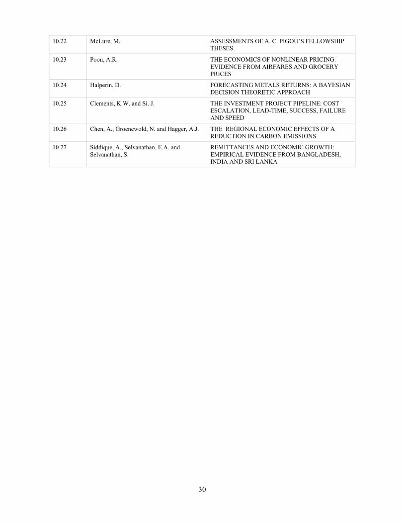
10.22 McLure, M. ASSESSMENTS OF A. C. PIGOU’S FELLOWSHIP THESES
10.23 Poon, A.R. THE ECONOMICS OF NONLINEAR PRICING: EVIDENCE FROM AIRFARES AND GROCERY PRICES
10.24 Halperin, D. FORECASTING METALS RETURNS: A BAYESIAN DECISION THEORETIC APPROACH
10.25 Clements, K.W. and Si. J. THE INVESTMENT PROJECT PIPELINE: COST ESCALATION, LEAD-TIME, SUCCESS, FAILURE AND SPEED
10.26 Chen, A., Groenewold, N. and Hagger, A.J. THE REGIONAL ECONOMIC EFFECTS OF A REDUCTION IN CARBON EMISSIONS
10.27 Siddique, A., Selvanathan, E.A. and Selvanathan, S.
REMITTANCES AND ECONOMIC GROWTH: EMPIRICAL EVIDENCE FROM BANGLADESH, INDIA AND SRI LANKA

31
ECONOMICS DISCUSSION PAPERS
2011 DP NUMBER
AUTHORS TITLE
11.01 Robertson, P.E. DEEP IMPACT: CHINA AND THE WORLD ECONOMY
11.02 Kang, C. and Lee, S.H. BEING KNOWLEDGEABLE OR SOCIABLE? DIFFERENCES IN RELATIVE IMPORTANCE OF COGNITIVE AND NON-COGNITIVE SKILLS
11.03 Turkington, D. DIFFERENT CONCEPTS OF MATRIX CALCULUS
11.04 Golley, J. and Tyers, R. CONTRASTING GIANTS: DEMOGRAPHIC CHANGE AND ECONOMIC PERFORMANCE IN CHINA AND INDIA
11.05 Collins, J., Baer, B. and Weber, E.J. ECONOMIC GROWTH AND EVOLUTION: PARENTAL PREFERENCE FOR QUALITY AND QUANTITY OF OFFSPRING
11.06 Turkington, D. ON THE DIFFERENTIATION OF THE LOG LIKELIHOOD FUNCTION USING MATRIX CALCULUS
11.07 Groenewold, N. and Paterson, J.E.H. STOCK PRICES AND EXCHANGE RATES IN AUSTRALIA: ARE COMMODITY PRICES THE MISSING LINK?
11.08 Chen, A. and Groenewold, N. REDUCING REGIONAL DISPARITIES IN CHINA: IS INVESTMENT ALLOCATION POLICY EFFECTIVE?
11.09 Williams, A., Birch, E. and Hancock, P. THE IMPACT OF ON-LINE LECTURE RECORDINGS ON STUDENT PERFORMANCE
11.10 Pawley, J. and Weber, E.J. INVESTMENT AND TECHNICAL PROGRESS IN THE G7 COUNTRIES AND AUSTRALIA
11.11 Tyers, R. AN ELEMENTAL MACROECONOMIC MODEL FOR APPLIED ANALYSIS AT UNDERGRADUATE LEVEL
11.12 Clements, K.W. and Gao, G. QUALITY, QUANTITY, SPENDING AND PRICES
11.13 Tyers, R. and Zhang, Y. JAPAN’S ECONOMIC RECOVERY: INSIGHTS FROM MULTI-REGION DYNAMICS
11.14 McLure, M. A. C. PIGOU’S REJECTION OF PARETO’S LAW
11.15 Kristoffersen, I. THE SUBJECTIVE WELLBEING SCALE: HOW REASONABLE IS THE CARDINALITY ASSUMPTION?
11.16 Clements, K.W., Izan, H.Y. and Lan, Y. VOLATILITY AND STOCK PRICE INDEXES
11.17 Parkinson, M. SHANN MEMORIAL LECTURE 2011: SUSTAINABLE WELLBEING – AN ECONOMIC FUTURE FOR AUSTRALIA
11.18 Chen, A. and Groenewold, N. THE NATIONAL AND REGIONAL EFFECTS OF FISCAL DECENTRALISATION IN CHINA
11.19 Tyers, R. and Corbett, J. JAPAN’S ECONOMIC SLOWDOWN AND ITS GLOBAL IMPLICATIONS: A REVIEW OF THE ECONOMIC MODELLING
11.20 Wu, Y. GAS MARKET INTEGRATION: GLOBAL TRENDS AND IMPLICATIONS FOR THE EAS REGION
32
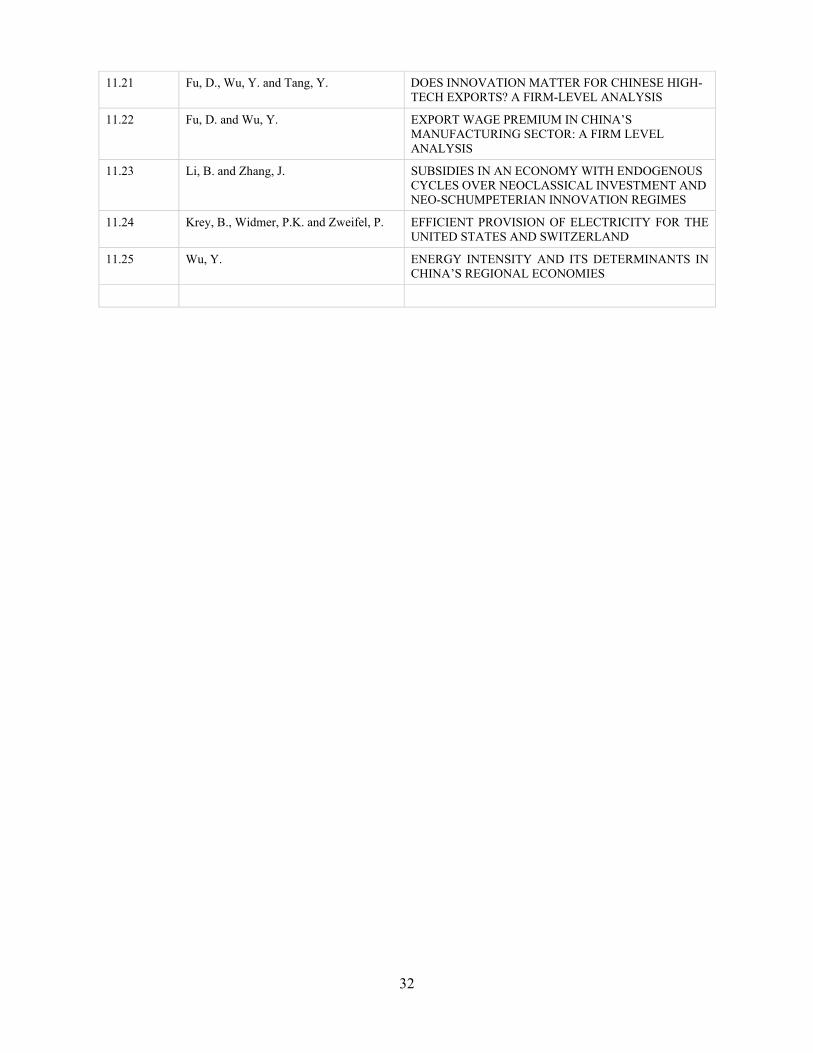
11.21 Fu, D., Wu, Y. and Tang, Y. DOES INNOVATION MATTER FOR CHINESE HIGH-TECH EXPORTS? A FIRM-LEVEL ANALYSIS
11.22 Fu, D. and Wu, Y. EXPORT WAGE PREMIUM IN CHINA’S MANUFACTURING SECTOR: A FIRM LEVEL ANALYSIS
11.23 Li, B. and Zhang, J. SUBSIDIES IN AN ECONOMY WITH ENDOGENOUS CYCLES OVER NEOCLASSICAL INVESTMENT AND NEO-SCHUMPETERIAN INNOVATION REGIMES
11.24 Krey, B., Widmer, P.K. and Zweifel, P. EFFICIENT PROVISION OF ELECTRICITY FOR THE UNITED STATES AND SWITZERLAND
11.25 Wu, Y. ENERGY INTENSITY AND ITS DETERMINANTS IN CHINA’S REGIONAL ECONOMIES


