1
Through the Kaleidoscope;Symmetries, Groups and
Chebyshev Approximationsfrom a Computational Point of View
H. Z. Munthe-Kaas, M. Nome and B. N. Ryland
Dept. of Mathematics, Univ. of Bergen, P.O. Box 7800, 5020 Norway
Abstract
In this paper we survey parts of group theory, with emphasis on struc-
tures that are important in design and analysis of numerical algorithms
and in software design. In particular, we provide an extensive introduc-
tion to Fourier analysis on locally compact abelian groups, and point to-
wards applications of this theory in computational mathematics. Fourier
analysis on non-commutative groups, with applications, is discussed more
briefly. In the final part of the paper we provide an introduction to multi-
variate Chebyshev polynomials. These are constructed by a kaleidoscope
of mirrors acting upon an abelian group, and have recently been applied
in numerical Clenshaw–Curtis type numerical quadrature and in spec-
tral element solution of partial differential equations, based on triangular
and simplicial subdivisions of the domain.
1.1 Introduction
Group theory is the mathematical language of symmetry. As a mature
branch of mathematics, with roots going almost two centuries back, it
has evolved into a highly technical discipline. Many texts on group theory
and representation theory are not readily accessible to applied mathe-
maticians and computational scientists, and the relevance of group the-
oretical techniques in computational mathematics is not widely recog-
nized.

2 H. Munthe-Kaas et. al.
Nevertheless, it is our conviction that knowledge of central parts of
group theory and harmonic analysis on groups is invaluable also for
computational scientists, both as a language to unify, analyze and gen-
eralize computational algorithms and also as an organizing principle of
mathematical software construction.
The first part of the paper provides a quite detailed self contained in-
troduction to Fourier analysis in the language of compact abelian groups.
Abelian groups are fundamental structures of major importance in com-
putations as they describe spaces with commutative shift operations.
Both continuous and discrete abelian groups are omnipresent as compu-
tational domains in applied mathematics. Classical Fourier analysis can
be understood as the theory of linear operators which commute with
translations in space; examples being differential operators with con-
stant coefficients, and other linear operators which are invariant under
change of time or space. A central theme in computation is the interplay
between continuous and discrete structures, between continuous mathe-
matical models and their discretizations. Many aspects of discretizations
can be understood via subgroups and sub-lattices of continuous abelian
groups. The duality between time/space and frequency/wave numbers
provided by the Fourier transform is another central topic which math-
ematically is expressed via Pontryagin duality of abelian groups.
Symmetries is a core topic of all group theory. Translation invariance
of linear operators is one type of symmetry. Another kind of symmetry
is invariance of operators under isometries acting upon the domain, e.g.
reflection symmetries. In the second part of this paper we will discuss
the importance of certain kaleidoscopic groups generated by a set of
mirrors acting upon a domain. We will review basic properties of mul-
tivariate versions of Chebyshev polynomials, which are constructed by
the folding of exponential functions under the action of kaleidoscopes.
Theoretically these have remarkable properties, both from an approxi-
mation theoretical point of view and also with respect to computational
complexity. However, until recently they have not been applied in com-
putations, probably due to the quite complicated underlying theory. We
will briefly review recent work where multivariate Chebyshev polynomi-
als are applied in numerical quadrature and in spectral element solution
of PDEs, and discuss some advantages and difficulties in this line of
work.
Through the Kaleidoscope 3
1.2 Fourier analysis on groups
Classical Fourier analysis is intimately connected with the theory of lo-
cally compact abelian groups. In mathematical analysis this view allows
a unified presentation of the Fourier transform, Fourier series and the dis-
crete Fourier transform [31]. In computational science, some understand-
ing of the group structures underlying discrete and continuous Fourier
analysis is invaluable both as a language to discuss computational as-
pects of Fourier transforms and sampling theory, as well as an organizing
principle of mathematical software [14]. In this section we provide a self-
contained review of Fourier analysis on abelian groups. We conclude this
section with a brief discussion on generalized Fourier transforms on non-
abelian groups and point to some applications of representation theory
in computational science. We refer to [5, 7, 11, 15, 16, 27, 31, 33] for
more details on the topics of this chapter.
1.2.1 Locally compact abelian groups
A Locally Compact Abelian group (LCA) is a locally compact topolog-
ical space G which is also an abelian group. Thus G has an identity
element 0, a group operation + and a unary − operation, such that
a+ b = b+a, a+(b+ c) = (a+ b)+ c and a+(−a) = 0 for all a, b, c ∈ G.
For our discussion it suffices to consider the elementary LCAs and groups
isomorphic to one of these:
Definition 1.1 The elementary LCAs are:
• The reals R under addition, with the standard definition of open sets.
• The integers Z under addition (with the discrete topology). This is
also known as the infinite cyclic group.
• The 1-dimensional torus, or circle T = R/2πZ defined as [0, 2π) ⊂ Runder addition modulo 2π, with the circle topology.
• The cyclic group of order k, Zk = Z/kZ, which consists of the integers
0, 1, . . . , k − 1 under addition modulo k (with the discrete topology).
• Direct products of the above spaces, G×H, in particular Rn (real
n-space), Tn (the n-torus) and all finitely generated abelian groups.
It is often convenient to consider these groups in their isomorphic
multiplicative form. E.g. the multiplicative group of complex numbers
of modulus 1, denoted T = { z ∈ C | |z| = 1 } is isomorphic to T via the
exponential map T 3 θ 7→ exp(iθ) ∈ T. More generally, ifG is an additive
abelian group with elements λ, we denote a corresponding multiplicative
4 H. Munthe-Kaas et. al.
group as eG with elements eλ, multiplicative group operation eλeλ′
=
eλ+λ′ and unit 1 = e0. The exponential notation is here just a formal
change of notation, a ‘syntactic sugar’ to simplify certain calculations.
An LCA with a finite subset of generators is called a Finitely Gen-
erated Abelian group (FGA). These, and in particular the finite ones,
are the basic domains of computational Fourier analysis and the Fast
Fourier Transform. A complete classification of these is simple and very
useful:
Theorem 1.2 (Classification of FGA) If G is an FGA, then G is
isomorphic to a group of the form
Zn×Zpn00×Zpn1
1×· · ·×Z
pnk−1k−1
(1.1)
where pi are primes, p0 ≤ p1 ≤ · · · ≤ pn−1 and ni ≤ ni+1 whenever
pi = pi+1. Furthermore G is also isomorphic to a group of the form
Zn×Zm0×Zm1
×· · ·×Zm`−1(1.2)
where mi divides mi+1. In both forms the representation is unique, i.e.
two FGA are isomorphic iff they can be transformed into the same canon-
ical form1.
1.2.2 Dual groups and the Fourier transform
Group homomorphisms are fundamental in describing sampling theory,
fast Fourier transforms and convolution theorems.
Definition 1.3 For two LCA H and G, we let hom(H,G) denote the
set of continuous homomorphisms from H to G, i.e. all continuous maps
φ : H → G such that
φ(h+ h′) = φ(h) + φ(h′) for all h, h′ ∈ H.
In particular χ ∈ hom(G,T) are homomorphisms into the multiplica-
tive group of complex numbers with modulus 1, defined as χ(x) = eiθ(x),
where θ ∈ hom(G,R). These homomorphisms χ are called the charac-
ters of G. The characters are always given by exponential maps and form
the basis for the Fourier transform. For two characters χ, χ′ it is clear
that the product (χχ′)(g) = χ(g)χ′(g) is also a character, and also the
complex conjugate χ is a character, which is the multiplicative inverse
of χ. Thus hom(G,T) is an abelian group called the dual group of G,
1 The isomorphisms are provided by the Chinese remainder theorem.
Through the Kaleidoscope 5
denoted G. With the compact-open topology G is also an LCA, thus,
we can define the double dualG. Pontryagin’s duality theorem states
that G andG are isomorphic LCAs. Due to this symmetry, we adopt a
slightly different definition of dual LCAs. In the following, we consider
both G and G as additive abelian groups and define the duality between
these via a dual pairing.
Definition 1.4 (Dual pair) Two LCAs G and G are called a dual pair
of LCAs if there exists a continuous function 〈·, ·〉 : G×G→ T such that
hom(G,T) ={〈k, ·〉 | k ∈ G
}hom(G,T) = { 〈·, x〉 | x ∈ G }.
The definition implies that
〈k + k′, x〉 = 〈k, x〉·〈k′, x〉 (1.3)
〈k, x+ x′〉 = 〈k, x〉·〈k, x′〉 (1.4)
〈0, x〉 = 〈k, 0〉 = 1 (1.5)
〈k, x〉 = 〈−k, x〉 = 〈k,−x〉. (1.6)
Furthermore, if 〈k, x〉 = 1 for all k, then x = 0, and if 〈k, x〉 = 1 for all x
then k = 0. If we work with pairings on different groups G,H, we write
〈·, ·〉G and 〈·, ·〉H to distinguish them.
Every LCA has a translation invariant Haar measure, yielding an in-
tegral∫Gf(x)dµ which is uniquely defined up to a scaling. For Rn and
Tn, this is the standard integral, and for the discrete Zk and Z, it is the
sum over the elements. The characters are orthogonal under the inner
product defined by the Haar measure. L2(G) denotes square integrable
functions on G.
Definition 1.5 (Fourier transform) The Fourier transform is a uni-
tary2 map : L2(G)→ L2(G) given as
f(k) =
∫G
〈−k, x〉f(x)dx. (1.7)
There exists a constant C such that the inverse transform is given as
f(x) =1
C
∫G
〈k, x〉f(k)dk. (1.8)
Sometimes we will write F(f) or FG(f) instead of f .
2 Unitary up to a scaling.

6 H. Munthe-Kaas et. al.
Note that G is discrete if and only if G is compact. In this case the
inversion formula becomes a sum, and C =∫G
1dx = vol(G). The fol-
lowing table presents the dual pairs for the elementary groups R, T , Zand Zn.
G G 〈·, ·〉 f(·) f(·)x ∈ R ω ∈ R e2πiωx
∫∞−∞ e−2πiωxf(x)dx
∫∞−∞ e2πiωxf(ω)dω
x ∈ T k ∈ Z e2πikx∫ 1
0e−2πikxf(x)dx
∑∞k=−∞ e2πikxf(k)
j ∈ Zn k ∈ Zn e2πikjn
∑n−1j=0 e
−2πikjn f(j) 1
n
∑n−1k=0 e
2πikjn f(k)
Multidimensional versions are given by the componentwise formulae:
x = (x1, x2) ∈ G = G1×G2
k = (k1, k2) ∈ G = G1×G2
〈k, x〉 = 〈k1, x1〉·〈k2, x2〉
f(k1, k2) =
∫G1
∫G2
〈−k1, x1〉〈−k2, x2〉f(x1, x2)dx1dx2
f(x1, x2) =1
C1C2
∫G1
∫G2
〈k1, x1〉〈k2, x2〉f(k1, k2)dk1dk2.
We end this section with a brief discussion of shifts and the convolu-
tion theorem. For a finite group G, we let CG denote the group algebra
(or group ring). This is the complex vector space of dimension |G|, where
each element in G is a basis vector, and with a product given by con-
volution. The convolution is most easily computed if we write the basis
vector for λ ∈ G in the multiplicative form eλ. Then f ∈ CG is repre-
sented by the vector f =∑λ∈G f(λ)eλ and we obtain the convolution
f ∗g of f, g ∈ CG by computing their product and collecting equal terms
fg =∑λ∈G
f(λ)eλ∑λ′∈G
g(λ′)eλ′
=∑λ∈G
(f ∗ g)(λ)eλ,
where
(f ∗ g)(λ) =∑λ′∈G
f(λ′)g(λ− λ′). (1.9)
For a continuous group G, we can similarly understand CG as a func-
tion space of complex valued functions on G. Care must be taken in
order to define a suitable function space for which convolutions make
sense, but these issues will not be discussed in this paper, see [31]. All
results tacitly assume that we define an appropriate function space, e.g.
L2(G), where operations such as convolutions and Fourier transforms
are well-defined.
Through the Kaleidoscope 7
The continuous convolution is given for f, g ∈ CG as
(f ∗ g)(x) =
∫x′∈G
f(x′)g(x− x′)dx′. (1.10)
Arguably the most important property of the Fourier transform is that
it diagonalizes the convolution, i.e.
(f ∗ g)(ξ) = f(ξ)g(ξ) for all ξ ∈ G. (1.11)
The proof is a straightforward computation. It is worthwhile to notice
that it relies upon the property that the group characters are homomor-
phisms, i.e. 〈ξ, x+x′〉 = 〈ξ, x〉〈ξ, x′〉, and upon the translation invariance
of the integral.
Similar results hold for more general non-commutative groups, in
which case the characters are replaced by group representations. Irre-
ducible group representations are matrix valued group homomorphisms
which form an orthogonal basis for L2(G), stated by the Frobenius the-
orem for finite G and Peter–Weyl theorem for compact G. Applications
of such generalized Fourier transforms in numerical linear algebra are
discussed in [2].
1.2.3 Subgroups, lattices and sampling
A subgroup of G, written H < G, is a topologically closed subset H ⊂ Gthat is closed under the group operations + and −.
Definition 1.6 For a subgroup H < G we define the annihilator sub-
group H⊥ < G as
H⊥ ={k ∈ G | 〈k, h〉G = 1 for all h ∈ H
}.
Note that if k, k′ ∈ G are such that k − k′ ∈ H⊥, then 〈k, h〉G =
〈k′, h〉G for all h ∈ H. This phenomenon is called aliasing in signal
processing, the two characters corresponding to k and k′ are indistin-
guishable when restricted to H.
Since G is abelian we can always form the quotient group K = G/H,
where the elements of K are the cosets H + g with the group operation
(H + g) + (H + g′) = H + g + g′, and the identity element of K is H.
Similarly, we can form the quotient H/H⊥, where each coset H⊥ + k
consists of a set of characters aliasing on H.
Definition 1.7 A lattice in G is a discrete subgroup H < G such that
G/H is compact.
8 H. Munthe-Kaas et. al.
An example is G = R, H = Z and K = R/Z = T . Also Z×Z < R×Ris a lattice. However, Z × 0 < R × R is not a lattice since the quotient
T ×R is not compact. If G is a finite group, then any H < G is a lattice.
As another example, consider G = Z with the lattice 2Z < G consist-
ing of all even integers. Theorem 1.2 states that 2Z is isomorphic to Zas an abstract group, thus it seems natural to define H = Z and identify
H with a subgroup of G via a group homomorphism φ0 ∈ hom(H,G)
given as φ0(j) = 2j. Similarly the quotient is K = Z2, identified with
the cosets of H in G via φ1 ∈ hom(G,K) given as φ1(j) = j mod 2,
where two elements j, j′ ∈ G belong to the same coset iff φ1(j− j′) = 0.
It is in general easy to define which properties of φ1 ∈ hom(H,G)
and φ2 ∈ (G,K) are necessary and sufficient for H to be (isomor-
phic to) a subgroup of G with quotient (isomorphic to) K. Recall that
the kernel and image of φ ∈ hom(G1, G2) are defined as ker(φ) =
{x ∈ G1 | φ(x) = 0 } and im(φ) = φ(G1) ⊂ G2. A (co)chain complex
is a sequence {Gj , φj} of homomorphisms between abelian groups φj ∈hom(Gj , Gj+1) such that im(φj) ⊂ ker(φj+1) for all j, in other words
φj+1◦φj = 0 for all j. The sequence is exact if ker(φj+1) = im(φj). A
short exact sequence is an exact sequence of five terms of the form
0 // Hφ0 // G
φ1 // K // 0 . (1.12)
The leftmost and rightmost arrows are the trivial maps 0 7→ 0 and
K 7→ 0. A short exact sequence defines a subgroup H < G with quo-
tient K = G/H, or more precisely φ0 is a monomorphism (injective
homomorphism) identifying H with a subgroup φ0(H) < G and φ1 an
epimorphism (surjective homomorphism) identifying G/φ0(H) with K.
Henceforth we will always define H as a subgroup of G with quotient K
by explicitly defining a short exact sequence and the maps φ0 and φ1.
Although this homological algebra point of view is ubiquitous in many
areas of pure mathematics, it is not a commonly used language in ap-
plied and computational mathematics. However, this presentation is also
very important from a computational point of view. First of all, this lan-
guage allows for a general and unified discussion of sampling, interpola-
tion and Fast Fourier Transforms. Furthermore, from an object oriented
programming point of view, it is an advantage to characterize mathe-
matical objects in terms of categorical diagrams. Classes in an object
oriented program consist of an internal representation of a certain ab-
straction as well as an interface defining the interaction and relationship
between different objects. Category theory and homological algebra is
Through the Kaleidoscope 9
thus a language which is important in defining classes in object oriented
programming. We will not discuss implementations further here, but re-
fer to [1, 14] for examples of this line of ideas within numerical analysis.
To understand sampling theory and the FFT in a group language, we
need to define adjoint homomorphisms, similarly to adjoints of linear
operators.
Definition 1.8 Given two LCAs H and G with dual pairings 〈·, ·〉Hand 〈·, ·〉G. The adjoint of a homomorphism φ ∈ hom(H,G) is φ ∈hom(G, H) defined such that
〈ξ, φ(x)〉G = 〈φ(ξ), x〉H for all ξ ∈ G and x ∈ H.
The following fundamental theorem is proven by standard techniques
in homological algebra.
Theorem 1.9 A short sequence of LCAs
0 // Hφ0 // G
φ1 // K // 0 .
is exact if and only if the adjoint sequence
0 Hoo Gφ0oo K
φ1oo 0oo .
is exact.
Note that K is a subgroup of G with quotient G/K = H. Furthermore,
for any x ∈ H and for any k ∈ K, we have that 〈φ1(k), φ0(h)〉G =
〈k, φ1◦φ0(x)〉K = 〈k, 0〉K = 1, since the composition of any two adjacent
arrows is 0. The exactness of the adjoint sequence implies that if ξ ∈ Gis such that 〈ξ, φ0(h)〉G = 0 for all h ∈ H, then ξ = φ1(k) for some
k ∈ K. Thus Theorem 1.9 implies the fundamental dualities
H < G, K = G/H,
H = G/K, K = H⊥ < G.
For many computational problems it is necessary to choose represen-
tative elements from each of the cosets in the quotient groups G/H and
G/K. E.g. in sampling theory, all characters in a coset K + ξ ⊂ G alias
on H, but physical relevance is usually given to the character ξ′ ∈ K+ ξ
which is closest to 0 (the lowest frequency mode). Similarly, we often
represent G/H by picking a representative from each coset, e.g. R/2πZcan be represented by [0, 2π) ⊂ R. The quotient map φ1 : G→ K assigns
each coset to a unique element in K, and we need to decide on a right
inverse of this map.

10 H. Munthe-Kaas et. al.
Definition 1.10 (Transversal of coset map) Given the short exact
sequence (1.12), a function σ : K → G is called a transversal of the
quotient map φ1 : G→ K if φ1◦σ = IdK .
Note that in general we cannot choose σ as a group homomorphism
(only if G = H × K), but it can be chosen as a continuous function.
In most applications G has a natural norm (e.g. Euclidean distance)
and we can choose σ such that the coset representatives are as close
to the origin as possible, i.e. such that ||σ(k)|| ≤ ||σ(k) − h|| for all
h ∈ φ0(H). This choice is called a Voronoi transversal. It is usually
not uniquely defined on the boundary, and the treatment of points on
the boundary must be done with some care in many applications. If
H is a lattice in a continuous group G, then the closure of the image
σ(K) ⊂ G is a polyhedron limited by hyperplanes halfway between 0
and its neighbouring lattice points. In sampling theory one usually picks
out the coset representatives for aliasing characters in G/K by letting
σ : H → G be the Voronoi transversal of φ0 with respect to the L2 norm
on G.
In the rest of this section, we assume that H,G and K form a short
exact sequence as in (1.12), where H is a lattice, i.e. H is discrete and
K is compact. Then H is compact and K = H⊥ is discrete, so H⊥ is a
lattice in G, called the reciprocal lattice. For a function f ∈ CG, we let
fH = f◦φ0 ∈ CH denote the function f downsampled to the lattice H.
Similarly, fH⊥ = f◦φ1 ∈ CH⊥.
Lemma 1.11 (Poisson summation formula) Given a lattice H < G
with reciprocal lattice H⊥ < G, there exists a constant C such that∑H
fH =1
C
∑H⊥
fH⊥ . (1.13)
If G is compact, then C = vol(G/H). With our normalization of the
Fourier transform on R, C = vol(G/H) also when G = Rn.
Proof Consider the group G/H via its set of coset representatives V :=
σ(K) ⊂ G. The characters of this group are {〈φ1(k), ·〉G}k∈K . Thus by
Fourier inversion in G/H there exists a constant C such that
f(0) = C∑k∈K
∫V
f(x)〈φ1(k), x〉Gdx.
We write x ∈ G as x = y + φ0(h), where y ∈ V , use 〈φ1(k), φ0(h)〉 ≡ 1
Through the Kaleidoscope 11
and the result above to obtain:∑k∈K
f◦φ1(k) =∑k∈K
∫G
f(x)〈φ1(k), x〉Gdx
=∑k∈K
∑h∈H
∫V
f(y + φ0(h))〈φ1(k), φ0(h) + y〉Gdy
=∑h∈H
∑k∈K
∫V
f(y + φ0(h))〈φ1(k), y〉Gdy
= C∑h∈H
f◦φ0(h).
If G is compact, we set f = 1 and compute f = vol(G)δ0. Since |H| =
vol(G)/vol(V ) we find C = vol(V ). The constant is computed for G =
Rn by considering the Fourier transform of f(x) = e−xT x, which under
an appropriate scaling, is invariant under the Fourier transform on Rn.
1.2.4 Heisenberg groups and the FFT
More material on topics related to this section is found in [4, 5, 35].
We can act upon f ∈ CG with a time-shift Sxf(t) := f(t + x) and
with a frequency shift χξf(t) := 〈ξ, t〉f(t). These two operations are dual
under the Fourier transform, but do not commute:
Sxf(ξ) = χxf(η) (1.14)
χξf(η) = S−ξ f(η) (1.15)
(Sxχξf) (t) = 〈ξ, x〉 · (χξSxf) (t). (1.16)
The full (non-commutative) group generated by time and frequency
shifts on CG is called the Heisenberg group of G.
The Heisenberg group of Rn is commonly defined as the multiplicative
group of matrices of the form 1 xT s
0 In ξ
0 0 1
,
where ξ, x ∈ Rn, s ∈ R. This group is isomorphic to the semidirect
product Rn × Rn oR where
(ξ′, x′, s′) · (ξ, x, s) = (ξ′ + ξ, x′ + x, s′ + s+ x′T ξ).
12 H. Munthe-Kaas et. al.
We prefer to instead consider Rn×RnoT (where T is the multiplicative
group consisting of z ∈ C such that |z| = 1) with product
(ξ′, x′, z′) · (ξ, x, z) = (ξ′ + ξ, x′ + x, z′ze2πix′T ξ).
More generally:
Definition 1.12 For an LCA G we define the Heisenberg group
HG = G×Go T with the semidirect product
(ξ′, x′, z′) · (ξ, x, z) = (ξ′ + ξ, x′ + x, z′ · z · 〈ξ, x′〉).
We define a left action HG × CG→ CG as follows
(ξ, x, z)·f = z · χξSxf. (1.17)
To see that this defines a left action, we check that (0, 0, 1) · f = f and
(ξ′, x′, z′) · ((ξ, x, z) · f) = ((ξ′, x′, z′) · (ξ, x, z)) · f.
Lemma 1.13 Let HG = G × G o T and HG = G × G o T act upon
f ∈ CG and f ∈ CG as in (1.17). Then
F((ξ, x, z) · f) = z · 〈−ξ, x〉 · χxS−ξ f = (x,−ξ, z · 〈−ξ, x〉) · f
Proof This follows from (1.14)–(1.16).
We will henceforth assume that H,G and K form a short exact se-
quence as in (1.12), with H discrete and K compact.
Definition 1.14 (Weil–Brezin map) The Weil–Brezin map WHG is
defined for f ∈ CG and (ξ, x, s) ∈ HG as
WHG f(ξ, x, z) =
∑H
((ξ, x, z) · f)H .
A direct computation shows that the Weil–Brezin map satisfies the
following symmetries for all (h′, h, 1) ∈ H⊥×H×1 ⊂ HG and all z ∈ T:
WHG f ((h′, h, 1) · (ξ, x, s)) =WH
G f(ξ, x, s) (1.18)
WHG f(ξ, x, z) = z · WH
G f(ξ, x, 1). (1.19)
Lemma 1.15 Γ = H⊥×H×1 is a subgroup of HG. It is not a normal
subgroup, so we cannot form the quotient group. However, as a manifold
the set of right cosets is
Γ\HG = H ×K × T.

Through the Kaleidoscope 13
The Heisenberg group has a right and left invariant volume measure
given by the direct product of the invariant measures of G, G and T.
Thus we can define the Hilbert spaces L2(HHG ) and L2(H ×K ×T). By
Fourier decomposition in the last variable (z-transform), L2(H×K×T)
splits into an orthogonal sum of subspaces Vk for k ∈ Z, consisting of
those g ∈ L2(H ×K × T) such that
g(ξ, x, z) = zkg(ξ, x, 1) for all z = e2πiθ.
It can be verified that WHG is unitary with respect to the L2 inner
product. Together with (1.18)–(1.19) this implies:
Lemma 1.16 The Weil–Brezin map is a unitary transform
WHG : L2(G)→ V1 ⊂ L2(H ×K × T).
Note that the Weil–Bezin map on G, with respect to the reciprocal
lattice H⊥, is
WH⊥
G: L2(G)→ V1 ⊂ L2(K × H × T).
The Poisson summation formula (Lemma 1.11) together with Lemma 1.13
implies that these two maps are related via
WHG f(ξ, x, z) =WH⊥
Gf(x,−ξ, z · 〈ξ, x〉).
Defining the unitary map J : L2 ⊂ L2(H ×K oT)→ L2(K × H ×T) as
Jf(x,−ξ, z · 〈ξ, x〉) = f(ξ, x, z), (1.20)
we obtain the following fundamental theorem.
Theorem 1.17 (Weil–Brezin factorization) Given an LCA G and a
lattice H < G. The Fourier transform on G factorizes in a product of
three unitary maps
FG =(WH⊥
G
)−1
◦J◦WHG . (1.21)
The Zak transform. Given a lattice H < G and transversals σ : K →G and σ : H → G. The Zak transform is defined as
ZHG f(ξ, x) :=WHG f(ξ, x, 1) for ξ ∈ σ(H), x ∈ σ(K). (1.22)
The Zak transform can be computed as a collection of Fourier transforms
on H of f shifted by x, for all x ∈ σ(K). The definition of the Fourier
transform yields:
ZHG f(−ξ, x) = FH ((Sxf)H) (φ0(ξ)). (1.23)
14 H. Munthe-Kaas et. al.
We see that the Zak transform is invertible when ZHG f(−ξ, x) is com-
puted for all ξ ∈ σ(H) and all x ∈ σ(K). Written in terms of the Zak
transform, the Weil–Brezin factorization (1.21) becomes
ZH⊥
Gf(x, ξ) = 〈ξ, x〉ZHG f(−ξ, x). (1.24)
The factor 〈ξ, x〉 is called a twiddle factor in the computational FFT
literature.
In the special case where G = H×K, then also K < G and H = K⊥.
Thus in this case it is possible to choose σ and σ as group homomor-
phisms, resulting in 〈ξ, x〉 ≡ 1 for all ξ ∈ σ(H) and x ∈ σ(K). This
choice is called a twiddle free factorization. However, by other choices of
the transversals, the twiddle factors also enter into the formula in this
case.
Due to the symmetries (1.18)–(1.19), the Weil–Brezin map is trivially
recovered from the Zak transform. The Zak transform is the practical
way of computing the Weil–Brezin map and its inverse. However, since
the invertible Zak transform cannot be defined canonically, indepen-
dently of the transversals σ and σ, the Weil–Brezin formulation is more
fundamental.
The Fast Fourier Transform. Cooley–Tukey style FFT algorithms
are based on recursive use of (1.24), where a Fourier transform on G
is computed by a collection of Fourier transforms on H composed with
inverse Fourier transforms on H⊥. We choose transversals σ and σ. If G
is finite, then σ(H) and σ(K) are finite. The Cooley–Tukey factorization
follows from (1.24):
• For each x ∈ σ(K) compute:
ZHG f(−ξ, x) = FH(Sxf)(φ0(ξ)) for all ξ ∈ σ(H) .
• For each ξ ∈ σ(H) compute:
f(ξ + φ1(κ)) = F−1H⊥
(〈ξ, σ(·)〉ZHG f(−ξ, σ(·))
)(κ) for all κ ∈ H⊥,
where the inverse Fourier transform F−1H⊥
is with respect to the vari-
able · ∈ K.
The Fast Fourier Transform is obtained by recursive application of this
splitting. This general formulation allows for Cooley–Tukey kind FFTs
based on any decomposition of G with respect to a lattice H. In par-
ticular this is useful for functions with symmetries, in which case it is
important to choose lattices H that preserve the symmetries in order to
Through the Kaleidoscope 15
take advantage of all the symmetries in the FFT. We return to this issue
in Section 1.3.4.
Shannon’s sampling theorem. By setting x = 0 in (1.24), we obtain
the important dual relationship between downsampling and periodiza-
tion:
FH(fH)(φ0(ξ)) =∑
k∈φ1(K)
FG(f)(k + ξ). (1.25)
A function f ∈ CG is band limited with respect to the reciprocal lattice
H⊥ if its Fourier transform is zero outside the Voronoi polyhedron, i.e.
if supp(f) ⊂ σ(H), where σ is a Voronoi transversal of φ0. If f is band
limited, the terms on the right hand side of (1.25) are zero for k 6= 0 and
ξ ∈ σ(H). This yields
FG(f)(ξ) = FH(fH)(φ0(ξ)),
thus we obtain Shannon’s celebrated result that a band limited f can
be exactly recovered from its downsampling fH .
Lattice rules. For general functions f ∈ CG, the error between the
Fourier transform of the true and the sampled function is given as
FH(fH)(φ0(ξ))−FG(f)(ξ) =∑
k∈φ1(K)\{0}
FG(f)(k + ξ).
The game of Lattice rules is, given f with specific properties, to find a
lattice H < G such that the error is minimised. We now assume that
the original domain is periodic G = Tn. Lattice rules are designed such
that the nonzero points in H⊥ neighbouring 0 are pushed as far out as
possible with respect to a given norm, depending on f . If f is spheri-
cally symmetric, H should be chosen as a densest lattice packing (with
respect to the 2-norm) [10], e.g. hexagonal lattice in R2 and face centred
cubic packing in R3 (as the orange farmers know well). In dimensions
up to 8, these are given by certain root lattices [30]. The savings, com-
pared to standard tensor product lattices, are given by the factors 1.15,
1.4, 2.0, 2.8 4.6, 8.0 and 16.0 in dimensions n = 2, 3, . . . , 8. This is im-
portant, but not dramatic, e.g. a camera with 8.7 megapixels arranged
in a hexagonal lattice has approximately the same sampling error as a
10 megapixel camera with a standard square pixel distribution. How-
ever, these alternative lattices have other attractive features, such as
larger spatial symmetry groups, yielding more isotropic discretizations.

16 H. Munthe-Kaas et. al.
A hexagonal lattice picture can be rotated more uniformly than a square
lattice picture.
Dramatic savings can be obtained for functions belonging to the Ko-
robov spaces. This is a common assumption in much work on high di-
mensional approximation theory. Korobov functions are functions whose
Fourier transforms have energy concentrated along the axis directions in
G, the so-called hyperbolic cross mass distribution. Whereas the tensor
product lattice with 2d points in each direction contains (2d)n lattice
points in Tn, the optimal lattice with respect to the Korobov norm con-
tains only O(2nd(log(d))n−1) points, removing exponential dependence
on d.
The group theoretical understanding of lattice rules makes software
implementation very clean and straightforward. In [29], numerical exper-
iments are reported on lattice rules for FFT-based spectral methods for
PDEs. Note that whereas the choice of transversal σ : H → G is irrele-
vant for lattice integration rules, it is essential for pseudospectral deriva-
tion. The Laplacian ∇2f is computed on G as f(ξ) 7→ c|ξ|2f(ξ), whereas
the corresponding computation on H must be done as FH(fH)(η) 7→c|σ(η)|2FH(fH)(η) for η ∈ H, and we must choose the Voronoi transver-
sal to minimise aliasing errors.
Polyhedral Dirichlet kernels. The theoretical understanding of lat-
tice sampling rules depends on the analytical properties of polyhedral
Dirichlet kernels. Let σ : H → G be the Voronoi transversal. The per-
fect low-pass filter DH ∈ CG is defined as
DH(ξ) =
{1 if ξ ∈ σ(H)
0 otherwise.
The polyhedral Dirichlet kernel DH ∈ CG is defined as
DH = F−1G (DH).
This function plays the same role as the classical Dirichlet kernel in the
1–dimensional sampling theory, e.g. low-pass reconstruction of a down
sampled function is done by convolution with DH . Detailed analysis of
these functions is done in [34, 36]. In particular it is important that they
in general have Lebesque constants scaling like O(logn(N)), where n is
the dimension of G, and N measures the number of sampling points in
H.
Through the Kaleidoscope 17
1.2.5 Fourier analysis on non-commutative groups
In this section we will briefly discuss computational aspects of Fourier
techniques on non-commutative groups. We will be much less detailed
than in the previous section, since this material is covered in detail
elsewhere, e.g. [3, 2, 30].
A starting point of the LCA discussion was the definition of the group
ring CG and the existence of a translation invariant measure, which
led to convolutions in the group ring. For non-commutative groups the
situation is a bit more complicated, since invariance with respect to
left and right translations might not yield the same measure. Groups
for which there exist a (unique up to scaling) measure which is both
left and right invariant is called unimodular. For such groups a lot of
the previous theory carries over, with some modifications. Groups which
are not unimodular are considerably more complicated and will not be
discussed here.
Important examples of unimodular groups are:
• Abelian groups.
• Finite groups.
• Compact groups.
• Semidirect product of compact and abelian groups, e.g. the Euclidean
motion group consisting of translations and rotations.
• Semisimple and nilpotent Lie groups.
Finite groups. Let CG denote the group ring, the complex vector space
of dimension |G|, where each element in G is a basis vector, so, as before,
f ∈ CG is given as f =∑g∈G f(g)g, where f(g) ∈ C. The right and left
invariant Haar measure is given as the sum over the elements∫G
fdµ =∑x∈G
f(x).
The product in G yields a convolution product in CG
(f ∗ g)(y) =∑x∈G
f(x)g(x−1y) =∑x∈G
f(yx)g(x−1).
This is, however, not a commutative product on CG, f ∗ g 6= g ∗ f .
In the abelian case, the Fourier transform diagonalizes the convolution
because the exponential basis consists of group homomorphisms (into
T). In the non-commutative case, it cannot be possible to diagonalize
the convolution using just hom(G,T) because the convolution is not
18 H. Munthe-Kaas et. al.
commutative. The idea of Schur and Frobenius in the late 19th cen-
tury was to look for a basis for CG in terms of group representations,
defined as elements of hom(G,U(n)), where U(n) is the set of unitary
n × n matrices. (Note that U(1) = T.) An n-dimensional representa-
tion is thus a function R : G → U(n) satisfying R(xy) = R(x)R(y)
and R(x−1) = R(x)−1 = R(x)†, where R(x)† is the complex conjugate
transpose. Let dR = n denote the dimension of the representation. For
each representation R, we may define Fourier coefficients of a function
f ∈ CG as a complex dR × dR matrix defined as
f(R) =∑x∈G
f(x)R(x)†.
A computation using the homomorphism property and shift invariance
of the sum, shows that the representations may be used to (block-
)diagonalize the convolution:
f ∗ g(R) = g(R)f(R). (1.26)
However, we need a basis for CG, and we need an inversion formula for
this generalised Fourier transform.
The concepts of equivalent and reducible representations are crucial
for constructing a suitable basis. Two representations R and R are equiv-
alent if there exists an invertible matrix V such that R(x) = V R(x)V −1
for all x. A representation is reducible if it is equivalent to a represen-
tation which is block-diagonal. In that case the representation can be
seen as a direct sum of smaller representations (one for each diagonal
block). Frobenius found that there always exists a complete list of non-
equivalent irreducible representations which forms an orthogonal basis
for CG.
Theorem 1.18 (Frobenius) For a finite group G there exists a com-
plete list of non-equivalent irreducible representations R = {R1, . . . , Rk}such that
∑R∈R d
2R = |G|. Define the generalized Fourier transform of
f ∈ CG as
f(R) =∑x∈G
f(x)R(x)† for all R ∈ R.
Then f is reconstructed by the formula
f(x) =1
|G|∑R∈R
dR trace(f(R)R(x)).

Through the Kaleidoscope 19
As an example, we consider the computation of the convolution of
f, g ∈ CG when G < O(3) is the icosahedral group, the collection of
the 120 orthogonal matrices which leave the icosahedron in R3 invari-
ant. This group has a complete list of irreducible representations of di-
mensions {1, 1, 3, 3, 3, 3, 4, 4, 5, 5}. A direct computation of the convolu-
tion involves 1202 multiplications. Instead, computing the convolution in
Fourier space involves the multiplication of matrices of size 1, 1, 3, 3, . . .,
which requires only 120 multiplications, saving a factor 120. For the com-
putation of matrix exponentials and eigenvalues, the savings are more
dramatic; a direct computation costs 1203 operations, while the equiva-
lent computation in Fourier space costs 2+4·33 +2·43 +2·53 operations,
which is cheaper by a factor of about 3500.
A source of computational problems leading to group convolutions
is linear problems with spatial symmetries. Given a linear operator Lwhich commutes with a finite group of isometries acting upon the do-
main (e.g. the Laplacian on the sphere commutes with any group of
isometries, e.g. the discrete icosahedral group). Let L be discretized in a
symmetry preserving manner, such that the discrete L commutes with
the isometries in G. Then L can be described as a block-convolution, i.e.
L belongs to a group ring of the form Cm×mG. The blocks represent the
interaction between different orbits of the action of G on the domain. As
an example, if the space of spherical functions is discretized with 12,000
degrees of freedom, the full space splits into about 12, 000/120 = 100 dif-
ferent orbits under the action of the icosahedral group. The Laplacian
can then be represented as a block-convolution in C100×100G. Under the
generalized Fourier transform, the matrix becomes block-diagonal, with
blocks of sizes 100dR for dR ∈ {1, 1, 3, 3, . . . , 5}.The use of the generalized Fourier transform is important in various
computational tasks, such as eigenvalue problems, solutions of linear
equations and computations of matrix exponentials. Experience shows
that symmetry preserving discretizations and algorithms are not only
much faster than direct algorithms, but they are also often more ac-
curate, since preservation of symmetry tends to diminish the effect of
numerical round-off errors.
Compact groups. Compact groups, such as, for example, the group
of rotations SO(3), are in many respects quite similar to finite groups.
There exists a bi-invariant Haar measure and a space of functions L2(G)
with a convolution product. The Peter–Weyl theorem guarantees that
there exist a discrete, infinite family of irreducible unitary represen-
20 H. Munthe-Kaas et. al.
tations forming an orthogonal basis for L2(G). The Fourier transform
becomes an integral over G and the inversion formula is similar to the
finite case, although the sum here is over an infinite list R.
The representation theory of orthogonal groups has numerous applica-
tions in computational science and technology, an example being recent
work on Cryo-Electron microscopy [18, 19]. The basic problem here is
the reconstruction of a 3D molecular structure from a large collection of
2D projections of the molecule seen from unknown angles. Representa-
tion theory provides an important tool to analyze numerical algorithms
for this problem.
Euclidean motions. The Euclidean motion group of translations and
rotations on R3 is important in many technological applications. The
group E(3) = SO(3) oR3 is the semidirect product of a compact group
and an abelian group. Such groups are always unimodular, and the repre-
sentation theory is relatively simple. The irreducible representations on
E(3) are induced from the representations of the compact part, SO(3),
by a standard method called the method of small groups [33]. An exam-
ple of an application of Fourier analysis on E(3) is the problem of medical
image registration; Find the Euclidean motion which best matches two
different 3-D images of an object. This can be phrased as the question of
computing the maximum of the cross correlation (or phase correlation)
of the two images. The cross correlation is very similar to a convolution
and can be cheaply computed in Fourier space.
1.3 Multivariate Chebyshev polynomials incomputations
Univariate (classical) Chebyshev polynomials are ubiquitous in numeri-
cal analysis and computational science, due to their in many ways opti-
mal approximation properties and the tight relationship between Cheby-
shev approximations and fast cosine transforms. First and second kind
Chebyshev polynomials {Tk}∞k=0 and {Uk}∞k=0 are defined as
x = cos(θ)
Tk(x) = cos(kθ)
Uk(x) = sin((k + 1)θ)/ sin(θ).
In this section we will discuss the connection between Chebyshev ap-

Through the Kaleidoscope 21
proximations and group theory. Once the group theoretical view is es-
tablished, it will become clear that there exist certain interesting multi-
variate generalizations of Chebyshev polynomials. These share most of
the favorable properties of the univariate polynomials, and they are or-
thogonal on domains related to triangles and simplices. Bivariate Cheby-
shev polynomials were constructed independently by Koornwinder [25]
and Lidl [26] by folding exponential functions. Multidimensional gener-
alizations (the A2 family) appeared first in [13]. In [21] a general fold-
ing construction was presented. Characterization of such polynomials as
eigenfunctions of differential operators is found in [6, 25].
Our interest in these polynomials originates from their potential appli-
cations in computational approximation methods, in particular spectral
element methods and multidimensional quadrature. We have developed
the theory of their discrete orthogonality, triangular based Clenshaw–
Curtis type quadrature formulae, recursion formulae for computing spec-
tral derivations as well as software for the application of multivariate
Chebyshev polynomials in approximation, quadrature and PDE solu-
tion. Our exposition here will aim at giving an overview of the main
ideas. More detailed presentations are found in [30, 32, 9].
Spectral element methods are computational techniques for solving
PDEs where the domain of the equation is divided into a fixed collec-
tion of regularly shaped subdomains. On each subdomain a high order
polynomial space is constructed, and a global solution is obtained by
patching together local solutions, either in a strong sense by imposing
continuity conditions across subdomain boundaries, or in a weak sense by
variational formulations (discontinuous Galerkin methods). The advan-
tage of spectral element methods compared to its competitors (finite el-
ements, finite differences and finite volume methods) is the phenomenon
called spectral convergence. When an analytic function is approximated
by an Nth order polynomial, one may achieve errors decaying as e−N .
Thus spectral methods are particularly attractive when high accuracy is
important.
The drawbacks of spectral element methods are that high order poly-
nomial approximations must be constructed with care. Jim Wilkinson
famously demonstrated that high order polynomial interpolation in equi-
spaced points is a highly unstable process, due to the fact that the
Lebesgue constant of equi-spaced interpolation points grows exponen-
tially in N . Interpolation in Chebyshev zeros, or Chebyshev extremal
points, is on the other hand near optimally stable, as the Lebesque con-
stant in such points grows as O(log(N)). Another problem with spectral
22 H. Munthe-Kaas et. al.
element methods is inflexibility with respect to sub-domain divisions.
High order polynomial approximations are easy to construct on rectan-
gular subdomains (by tensor products of univariate polynomials), but
high order approximation theory based on triangular and tetrahedral
subdivisions is far less developed. The most common practice is there-
fore rectangular subdivision methods. Triangular and tetrahedral sub-
division schemes are far more flexible, if they can be implemented in an
efficient and stable manner. A singular mapping technique from squares
to triangles [12] is a possible solution, but has drawbacks in breaking of
triangular symmetries as well as other problems. Nodal spectral Galerkin
methods are another approach where good collocation nodes are com-
puted by numerical optimization (e.g. Fekete points). But in this ap-
proach one has no direct connection to Fourier analysis, and fast trans-
forms are not available [17, 20]. This makes spectral element methods
based on multivariate Chebyshev polynomials an attractive alternative.
We start with a discussion of particular eigenfunctions of the Laplacian
on simplices.
1.3.1 What is the sound of a triangular drum?
Bases for high order approximation spaces are usually obtained as eigen-
functions of Sturm–Liouville problems, truncated to a given order. Can
we find Sturm–Liouville problems on triangles and simplices, that yield
good approximation spaces? It is known that the eigenfunctions of the
Laplacian (with Dirichlet or Neumann boundary conditions) can be ex-
plicitly constructed on certain triangular domains in 2D and some par-
ticular simplices in all higher dimensions. An illustrative example is the
construction of Laplacian eigenfunctions on an equilateral triangle, with
Dirichlet or Neumann boundary conditions.
The equilateral triangle has the particular property that if we set up
a kaleidoscope with three mirrors at the three edges, then the reflec-
tions of the triangle tile the plane in a periodic pattern, shown as the
shaded domain in the right part of Figure 1.2 (labelled A2). Without
loss of generality, we assume that the triangle has corners in the origin
[0; 0], λ1 = [1/√
2; 1/√
6] and λ2 = [0;√
2/√
3]. Let {sj}3j=1 denote re-
flections of R2 about the edges of the triangle. Let W denote the full
group of isometries of R2 generated by {sj}3j=1. This is an example of a
crystallographic group3, a group of isometries of Rd where the subgroup
3 More specifically it is an affine Weyl group, to be defined below.

Through the Kaleidoscope 23
of translations form a lattice in Rd. From this fact we will derive the
Laplacian eigenfunctions on the triangle, which we denote by 4.
The translation lattice of W is L = spanZ{α1, α2} < R2 generated
by the vectors α1 = (√
2, 0) and α2 = (−1/√
2,√
3/√
2). The unit cell
of L can be taken as either the rhombus spanned by α1 and α2 or the
hexagon 9 indicated in Figure 1.2. The hexagon is the Voronoi cell of
the origin in the lattice L, its interior consists of the points in R2 that
are closer to the origin than to any other lattice points. As a first step in
our construction of triangular eigenfunctions, we consider the L-periodic
eigenfunctions of the Laplacian ∇2. Since (λj , αk) = δj,k, the reciprocal
lattice is L⊥ = spanZ{λ1, λ2} and the periodic eigenfunctions are
∇2t 〈λ, t〉 = −(2π)2||λ||2〈λ, t〉 for all λ ∈ L⊥, t ∈ R2/L,
where 〈λ, t〉 = e2πi(λ,t) is the dual pairing on R2. We continue to find the
Laplacian eigenfunctions on 4 by folding the exponentials. Let W < W
be the subgroup which leaves the origin fixed (the symmetries of 9):
W = {e, s1, s2, s1s2, s2s1, s1s2s1},
where e is the identity and si, i ∈ {1, 2} act on v ∈ R2 as siv = v −2(αi, v)/(αi, αi). We define even and odd (cosine and sine-type) foldings
of the exponentials
cλ(t) =1
|W |∑w∈W
〈λ,wt〉 =1
|W |∑w∈W
⟨wTλ, t
⟩(1.27)
sλ(t) =1
|W |∑w∈W
det(w) 〈λ,wt〉 =1
|W |∑w∈W
det(w)⟨wTλ, t
⟩,(1.28)
where, in our example, |W | = 6. The Laplacian commutes with any
isometry, in particular ∇2(f ◦w) = (∇2f) ◦w for w ∈W . Hence, the re-
flected exponentials and the functions cλ(t) and sλ(t) are eigenfunctions
with the same eigenvalue:
Lemma 1.19 The eigenfunctions of ∇2 on the equilateral triangle 4with Dirichlet (f = 0) and Neumann boundary conditions (∇f · ~n = 0)
are given respectively as
∇2t cλ(t) = −(2π)2||λ||2cλ(t)
∇2t sλ(t) = −(2π)2||λ||2sλ(t),
for λ ∈ spanN{λ1, λ2}, the set of all non-negative integer combinations
of λ1 = [1/√
2; 1/√
6] and λ2 = [0;√
2/√
3].
24 H. Munthe-Kaas et. al.
The set spanN{λ1, λ2} ⊂ L⊥ contains exactly one point from each W -
orbit, and is called the positive Weyl chamber. An important question
is how good (or bad!) these eigenfunctions are as bases for approximat-
ing analytic functions on 4. It is well known from the univariate case
that the similar construction, yielding the eigenfunctions cos(kθ) and
sin(kθ) on [0, π] are not giving a basis converging at a super-algebraic
speed. For an analytic function f(θ) where f(0) = f(π) = 0, the even
2π-periodic extension is piecewise smooth, with only C0 continuity at
θ ∈ {0, π}. Hence the Fourier-cosine series converges only as O(k−2).
There are several different ways to achieve the desired O(exp(−ck))
spectral convergence rate for analytic functions. One possible solution
is to approximate f(θ) in a frame (not linearly independent) consisting
of both {cos(kθ)}k∈Z and {sin(kθ)}k∈Z+ [22]. Another possibility is to
employ a change of variable x = cos(θ), yielding (univariate) Chebyshev
polynomials with spectral convergence. Here we will discuss a gener-
alization of the latter approach leading to the multivariate Chebyshev
polynomials.
1.3.2 Through the kaleidoscope
Recall that the main trick for finding eigenfunctions of the Laplacian on
the triangle was in using the fact that the domain is a polyhedron with
the property that the group generated by the boundary reflections is a
crystallographic group, defined as a group of isometries on Rn such that
the subgroup of translations form a lattice L < Rn. Crystallographic
groups is a classical topic of mathematics, physics and chemistry. A
classification of such groups starts with the fundamental crystallographic
restriction: For any crystallographic group, the only allowed rotations
are 2-fold, 3-fold, 4-fold and 6- fold4. A general group generated just
by reflections, as in a kaleidoscope, is called a Coxeter group, and the
Coxeter groups which comply with the crystallographic restriction are
called affine Weyl groups. These are classified in terms of their root
systems, where the roots are orthogonal to the mirrors passing through
the origin.
Root systems. Let V be a finite dimensional real Euclidean vector
space with standard inner product (·, ·). The construction above can
4 The 5-fold symmetry is not allowed in proper crystals, but is seen inquasicrystals, related to Penrose tilings. This discovery was the topic of the 2011Nobel prize in chemistry.

Through the Kaleidoscope 25
Figure 1.1 Dynkin diagrams for irreducible root systems
be generalized to all those simplices 4 ⊂ V with the property that
the group of isometries W generated by reflecting 4 about its faces is
a crystallographic group. All such simplices are determined by a root
system, a set of vectors in V which are perpendicular to the reflection
planes of W passing through the origin. We review some basic definitions
and results about root systems. For more details we refer to [8].
Definition 1.20 A root system in V is a finite set Φ of non-zero
vectors, called roots, that satisfy:
1. The roots span V.
2. The only scalar multiples of a root α ∈ Φ that belong to Φ are α and
−α.
3. For every root α ∈ Φ, the set Φ is invariant under reflection through
the hyperplane perpendicular to α. I.e. for any two roots α and β,
the set Φ contains the reflection of β,
sα(β) := β − 2(α, β)
(α, α)α ∈ Φ.
4. (Crystallographic restriction): For any α, β ∈ Φ we have
2(α, β)
(α, α)∈ Z.
Condition 4 implies that the obtuse angle between two different re-
flection planes must be either 90◦, 120◦, 135◦ or 150◦. The rank of the
root system is the dimension d of the space V. Any root system contains
a subset (not uniquely defined) Σ ⊂ Φ of so-called simple positive roots.
This is a set of d linearly independent roots Σ = {α1, . . . , αd} such that
any root β ∈ Φ can be written either as a linear combination of αj with
26 H. Munthe-Kaas et. al.
non-negative integer coefficients, or as a linear combination with non-
positive integer coefficients. We call Σ a basis of the root system Φ. A
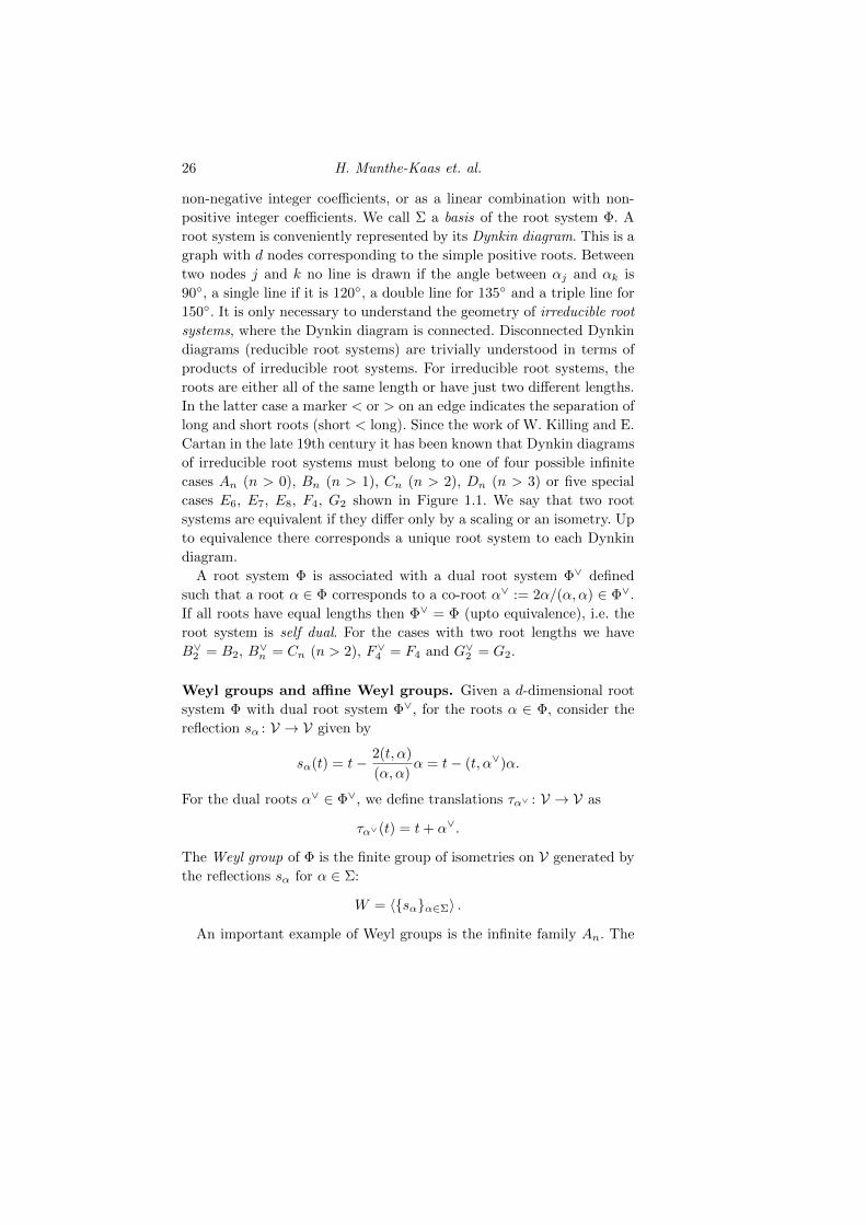
root system is conveniently represented by its Dynkin diagram. This is a
graph with d nodes corresponding to the simple positive roots. Between
two nodes j and k no line is drawn if the angle between αj and αk is
90◦, a single line if it is 120◦, a double line for 135◦ and a triple line for
150◦. It is only necessary to understand the geometry of irreducible root
systems, where the Dynkin diagram is connected. Disconnected Dynkin
diagrams (reducible root systems) are trivially understood in terms of
products of irreducible root systems. For irreducible root systems, the
roots are either all of the same length or have just two different lengths.
In the latter case a marker < or > on an edge indicates the separation of
long and short roots (short < long). Since the work of W. Killing and E.
Cartan in the late 19th century it has been known that Dynkin diagrams
of irreducible root systems must belong to one of four possible infinite
cases An (n > 0), Bn (n > 1), Cn (n > 2), Dn (n > 3) or five special
cases E6, E7, E8, F4, G2 shown in Figure 1.1. We say that two root
systems are equivalent if they differ only by a scaling or an isometry. Up
to equivalence there corresponds a unique root system to each Dynkin
diagram.
A root system Φ is associated with a dual root system Φ∨ defined
such that a root α ∈ Φ corresponds to a co-root α∨ := 2α/(α, α) ∈ Φ∨.
If all roots have equal lengths then Φ∨ = Φ (upto equivalence), i.e. the
root system is self dual. For the cases with two root lengths we have
B∨2 = B2, B∨n = Cn (n > 2), F∨4 = F4 and G∨2 = G2.
Weyl groups and affine Weyl groups. Given a d-dimensional root
system Φ with dual root system Φ∨, for the roots α ∈ Φ, consider the
reflection sα : V → V given by
sα(t) = t− 2(t, α)
(α, α)α = t− (t, α∨)α.
For the dual roots α∨ ∈ Φ∨, we define translations τα∨ : V → V as
τα∨(t) = t+ α∨.
The Weyl group of Φ is the finite group of isometries on V generated by
the reflections sα for α ∈ Σ:
W = 〈{sα}α∈Σ〉 .
An important example of Weyl groups is the infinite family An. The
Through the Kaleidoscope 27
Weyl group W of An is isomorphic to the symmetric group Sn+1. This
is a group of order |Sn+1| = (n + 1)!, consisting of all permutations
of n + 1 objects, and is also isomorphic to the symmetry group of the
regular n-simplex. In particular the Weyl group of A2 has order 6 and
can be identified with the symmetries of the regular triangle.
The dual root lattice L∨ is the lattice spanned by the translations τα∨
for α∨ ∈ Σ∨. We identify this with the abelian group of translations on
V generated by the dual roots
L∨ = 〈{τα∨}α∨∈Σ∨〉 .
The affine Weyl group W is the infinite crystallographic symmetry group
of V generated by the reflections sα for α ∈ Σ and the translations τα∨
for α∨ ∈ Σ∨, thus it is the semidirect product of the Weyl group W with
the dual5 root lattice L∨
W = 〈{sα}α∈Σ, {τα∨}α∨∈Σ∨〉 = W o L∨.
Let Λ = (L∨)⊥
denote the reciprocal lattice of L∨. The lattice Λ is
spanned by vectors {λj}dj=1 such that (λj , α∨k ) = δj,k for all α∨k ∈ Σ∨.
The vectors λj are called the fundamental dominant weights of the root
system Φ, and Λ is called the weights lattice.
The positive Weyl chamber C+ is defined as the closed conic subset
of V containing the points with nonnegative coordinates with respect to
the dual basis {λ1, . . . , λd}, in other words
C+ = {t ∈ V : (t, αj) ≥ 0}.
This is a fundamental domain for the Weyl group acting on V. The
boundary of C+ consists of the hyperplanes perpendicular to {α1, . . . , αd}.The affine Weyl group contains reflection symmetries about affine planes
perpendicular to the roots, shifted a half integer multiple of the length
of a co-root away from the origin, i.e. for each α∨ ∈ Φ∨ and each
k ∈ Z there is an affine plane consisting of the points Pk,α∨ = {t ∈V : 2(t, α∨) = k(α∨, α∨)} = {t ∈ V : (t, α) = k}, and this affine plane is
invariant under the affine reflection τkα∨ · sα. A connected closed subset
of V limited by such affine planes is called an alcove and is a fundamental
domain for the affine Weyl group W .
The situation is particularly simple for irreducible root systems, where
5 Since the Weyl groups of Φ and of Φ∨ are identical, it is no problem to instead
define W = W o L as the semidirect product of the Weyl group with the primalroot lattice. We have, however, chosen to follow the most common definitionhere, which leads to a slightly simpler notation for the Fourier analysis.

28 H. Munthe-Kaas et. al.
the alcoves are always d-simplices. Recall that all roots α ∈ Φ can be
written as α =∑dk=1 nkαk where all nk = 2(α, λk)/(αk, αk) are either
non-negative or all non-positive integers. A root α strictly dominates
another root α, written α � α, if nk ≥ nk for all k, with strict inequality
for at least one k. Irreducible root systems have a unique dominant root
α ∈ Φ such that α � α for all α 6= α. The dominant root α is the
unique long root in the Weyl chamber (possibly on the boundary). The
basic geometric properties of affine Weyl groups are summarized by the
following lemma:
Lemma 1.21
1 If Φ is irreducible with dominant root α then a fundamental domain
for W is the simplex 4 ⊂ V given as
4 = {t ∈ V : (t, α) ≤ 1 and (t, αj) ≥ 0 for all αj ∈ Σ},
where 4 has corners in the origin and in the points λj/(λj , α) for
j = 1, . . . , d.
2 The affine Weyl group is generated by the affine reflections about
the boundary faces of the fundamental domain 4. For irreducible Φ
these are
W = 〈{sαj}dj=1
, τα · sα〉.
3 If Φ is reducible then a fundamental domain for the affine Weyl
group is given as the Cartesian product of the fundamental domains
for each of its irreducible components.
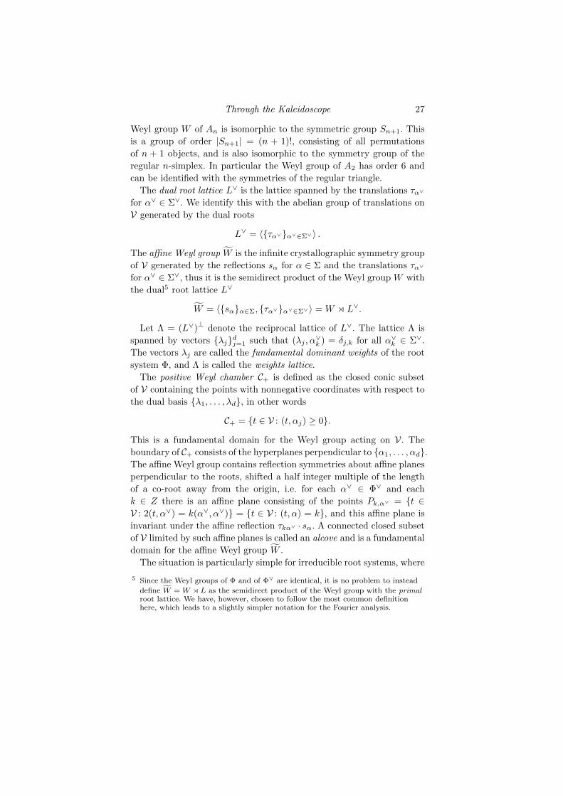
The simplest rank d root system is the reducible system A1×· · ·×A1,
where the Dynkin diagram consists of d non-connected dots. Figure 1.2
shows A1×A1. The solid black square is the fundamental domain of the
root lattice, and the small shaded square the fundamental domain of the
affine Weyl group W .
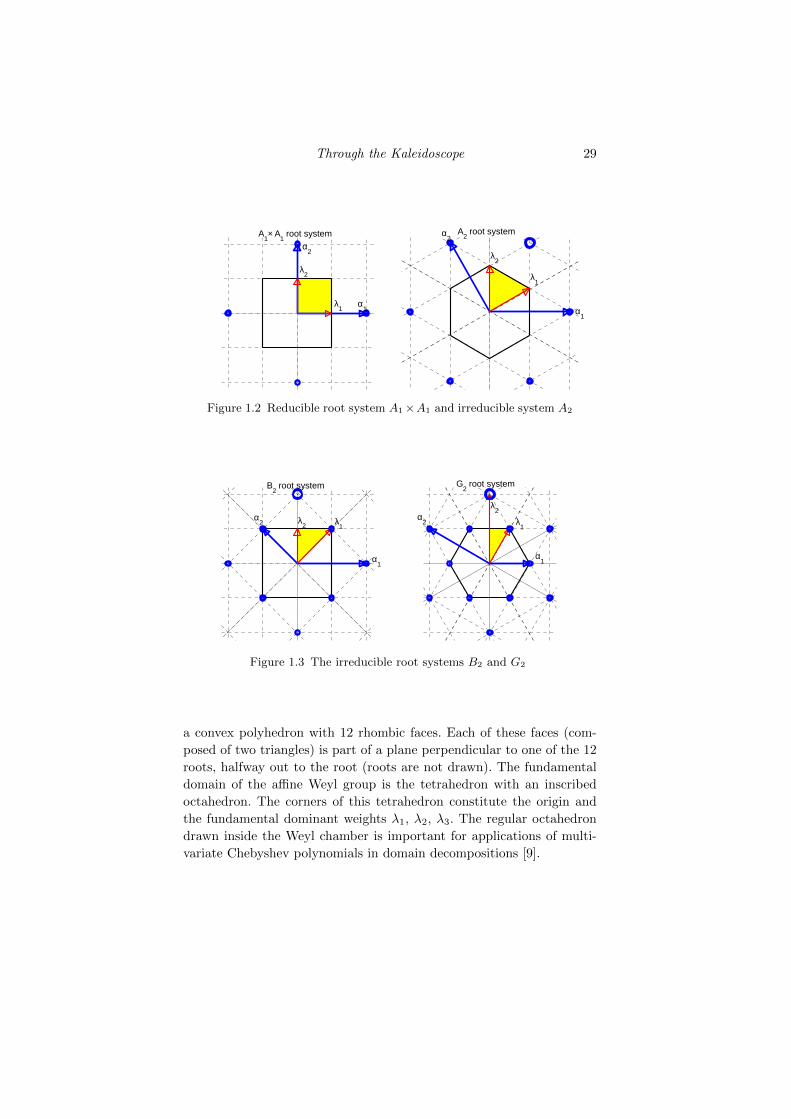
The right part of Figure 1.2 and Figure 1.3 shows the irreducible 2-d
cases with roots α (large dots), dominant root α (circle), simple positive
roots (α1, α2), and fundamental dominant weights (λ1, λ2). The roots
are normalized such that the longest roots have length√
2, thus for long
roots α∨ = α. For short roots we have for B2 that α∨ = 2α and for G2
that α∨ = 3α. The fundamental domain of the dual root lattice (Voronoi
region of L∨) is indicated by 9, � and 7, and the fundamental domain
for the affine Weyl group (an alcove) is indicated by shaded triangles.
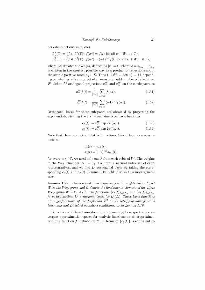
Figure 1.4 shows the A3 case (self dual), where the fundamental do-
main (Voronoi region) of the root lattice is a rhombic dodecahedron,
Through the Kaleidoscope 29
α1
α2
λ2
λ1
A1× A
1 root system α
2
α1
λ2
λ1
A2 root system
Figure 1.2 Reducible root system A1×A1 and irreducible system A2
B2 root system
λ1
λ2
α1
α2
G2 root system
α2
α1
λ2
λ1
Figure 1.3 The irreducible root systems B2 and G2
a convex polyhedron with 12 rhombic faces. Each of these faces (com-
posed of two triangles) is part of a plane perpendicular to one of the 12
roots, halfway out to the root (roots are not drawn). The fundamental
domain of the affine Weyl group is the tetrahedron with an inscribed
octahedron. The corners of this tetrahedron constitute the origin and
the fundamental dominant weights λ1, λ2, λ3. The regular octahedron
drawn inside the Weyl chamber is important for applications of multi-
variate Chebyshev polynomials in domain decompositions [9].

30 H. Munthe-Kaas et. al.
Figure 1.4 Fundamental domains of A3 root system
1.3.3 Laplacian eigenfunctions on triangles, tetrahedra
and simplices.
In this section we will consider real or complex valued functions on Vrespecting symmetries of an affine Weyl group. Consider first L2(T), the
space of complex valued L2-integrable periodic functions on the torus
T = V/L∨, i.e. functions f such that f(y + α∨) = f(y) for all y ∈ Vand α∨ ∈ L∨. Since the weights lattice Λ is reciprocal to L∨, the Fourier
transform and its inverse are given for f ∈ L2(T) as
f(λ) = F(f)(λ) =1
vol(T)
∫T
f(t)〈−λ, t〉dt, (1.29)
f(t) = F−1(f)(t) =∑λ∈Λ
f(λ)〈λ, t〉. (1.30)
We are interested in functions which are both periodic under translations
in L∨ and also respect the other symmetries in W , e.g. functions with
odd or even symmetry6 with respect to the reflections in W . Due to the
semi-direct product structure W = W o L∨ it follows that any W ∈ Wcan be written W = w · τα∨ , where w ∈ W and α∨ ∈ L∨. Thus on the
space of periodic functions L2(T), the action of W and the finite group
W are identical. We define subspaces of symmetric and skew-symmetric
6 There are other possible symmetries as well, related to other representations ofthe Weyl group [9].
Through the Kaleidoscope 31
periodic functions as follows
L2∨(T) = {f ∈ L2(T): f(wt) = f(t) for all w ∈W , t ∈ T}
L2∧(T) = {f ∈ L2(T): f(wt) = (−1)|w|f(t) for all w ∈W , t ∈ T},
where |w| denotes the length, defined as |w| = `, where w = sαj1 · · · sαj`is written in the shortest possible way as a product of reflections about
the simple positive roots αj ∈ Σ. Thus (−1)|w| = det(w) = ±1 depend-
ing on whether w is a product of an even or an odd number of reflections.
We define L2 orthogonal projections πW∨ and πW∧ on these subspaces as
πW∨ f(t) =1
|W |∑w∈W
f(wt), (1.31)
πW∧ f(t) =1
|W |∑w∈W
(−1)|w|f(wt). (1.32)
Orthogonal bases for these subspaces are obtained by projecting the
exponentials, yielding the cosine and sine type basis functions
cλ(t) := πW∨ exp 2πi(λ, t) (1.33)
sλ(t) := πW∧ exp 2πi(λ, t). (1.34)
Note that these are not all distinct functions. Since they possess sym-
metries
cλ(t) = cwλ(t),
sλ(t) = (−1)|w|swλ(t),
for every w ∈W , we need only one λ from each orbit of W . The weights
in the Weyl chamber, Λ+ = C+ ∩ Λ, form a natural index set of orbit
representatives, and we find L2 orthogonal bases by taking the corre-
sponding cλ(t) and sλ(t). Lemma 1.19 holds also in this more general
case.
Lemma 1.22 Given a rank d root system φ with weights lattice Λ, let
W be the Weyl group and 4 denote the fundamental domain of the affine
Weyl group W = W o L∨. The functions {cλ(t)}λ∈Λ+and {sλ(t)}λ∈Λ+
form two distinct L2 orthogonal bases for L2(4). These basis functions
are eigenfunctions of the Laplacian ∇2 on 4 satisfying homogeneous
Neumann and Dirichlet boundary conditions, as in Lemma 1.19.
Truncations of these bases do not, unfortunately, form spectrally con-
vergent approximation spaces for analytic functions on 4. Approxima-
tion of a function f , defined on 4, in terms of {cλ(t)} is equivalent to
32 H. Munthe-Kaas et. al.
Fourier approximation of the even extension of f in L2∨(T), and we do in
general only observe quadratic convergence due to discontinuity of the
gradient across the boundary of4. A route to spectral convergence is by
a change of variables which turns the trigonometric polynomials {cλ(t)}and {sλ(t)} into multivariate Chebyshev polynomials of first and second
kind.
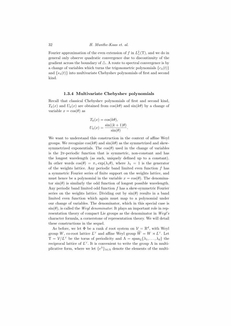
1.3.4 Multivariate Chebyshev polynomials
Recall that classical Chebyshev polynomials of first and second kind,
Tk(x) and Uk(x) are obtained from cos(kθ) and sin(kθ) by a change of
variable x = cos(θ) as
Tk(x) = cos(kθ),
Uk(x) =sin((k + 1)θ)
sin(θ).
We want to understand this construction in the context of affine Weyl
groups. We recognize cos(kθ) and sin(kθ) as the symmetrized and skew-
symmetrized exponentials. The cos(θ) used in the change of variables
is the 2π-periodic function that is symmetric, non-constant and has
the longest wavelength (as such, uniquely defined up to a constant).
In other words cos(θ) = π∨ exp(λ1θ), where λ1 = 1 is the generator
of the weights lattice. Any periodic band limited even function f has
a symmetric Fourier series of finite support on the weights lattice, and
must hence be a polynomial in the variable x = cos(θ). The denomina-
tor sin(θ) is similarly the odd function of longest possible wavelength.
Any periodic band limited odd function f has a skew-symmetric Fourier
series on the weights lattice. Dividing out by sin(θ) results in a band
limited even function which again must map to a polynomial under
our change of variables. The denominator, which in this special case is
sin(θ), is called the Weyl denominator. It plays an important role in rep-
resentation theory of compact Lie groups as the denominator in Weyl’s
character formula, a cornerstone of representation theory. We will detail
these constructions in the sequel.
As before, we let Φ be a rank d root system on V = Rd, with Weyl
group W , co-root lattice L∨ and affine Weyl group W = W o L∨. Let
T = V/L∨ be the torus of periodicity and Λ = spanZ{λ1, . . . , λd} the
reciprocal lattice of L∨. It is convenient to write the group Λ in multi-
plicative form, where we let {eλ}λ∈Λ denote the elements of the multi-
Through the Kaleidoscope 33
plicative group, understood as formal symbols such that for λ, µ ∈ Λ we
have eλ · eµ = eλ+µ.
Let E = E(C) ⊂ L2(Λ) denote the free complex vector space over the
symbols eλ. This consists of all formal sums a =∑λ∈Λ a(λ)eλ where
the coefficients a(λ) ∈ C and all but a finite number of these are non-
zero. An element a ∈ E is identified with a trigonometric polynomial
f(t) = F−1(a)(t) on the torus T (i.e. a band limited periodic function)
through the Fourier transforms given in (1.29)–(1.30).
Let EW∨ ⊂ E denote the symmetric subalgebra of those elements that
are invariant under the action of the Weyl group W on E . This consists
of those a ∈ E where a(λ) = a(wλ) for all λ and all w ∈ W . Similarly,
EW∧ ⊂ E denotes those a ∈ E that are alternating sign under reflections
sα, i.e. where the coefficients satisfy a(λ) = (−1)|w|a(wλ). Projections
πW∨ : E → E∨ and πW∧ : E → E∧ are defined as in (1.31)–(1.32).
The algebra E is generated by {eλj}dj=1 ∪ {e−λj}dj=1 where λj are the
fundamental dominant weights. EW∨ is the subalgebra generated by the
symmetric generators {zj}dj=1 defined as
zj = πW∨ eλj =
1
|W |∑w∈W
ewλj =2
|W |∑
w∈W+
ewλj , (1.35)
where W+ denotes the even subgroup of W containing those w such
that |w| is even. The latter identity follows from sαjλj = λj , thus it is
enough to consider only w of even length. The action of W+ on λj is
free and effective.
It can be shown that EW∨ is a unique factorization domain over the
generators {zj}, i.e. any a ∈ EW∨ can be expressed uniquely as a polyno-
mial in {zj}dj=1.
The skew subspace EW∧ does not form an algebra, but this can be
corrected by dividing out the Weyl denominator. Define the Weyl vector
ρ ∈ Λ as
ρ =
d∑j=1
λj =1
2
∑α∈Φ+
α.
We define the Weyl denominator D ∈ EW∧ as
D =∑w∈W
(−1)|w|ewρ.
Proposition 1 Any a ∈ EW∧ is divisible by D, i.e. there exist a unique
b ∈ EW∨ such that a = bD.
34 H. Munthe-Kaas et. al.
Proof See [8] Prop. 25.2.
Any a ∈ EW∨ can be written as a polynomial in z1, . . . , zd, hence the
following polynomials are well defined.
Definition 1.23 For λ ∈ Λ we define multivariate Chebyshev polyno-
mials of first and second kind Tλ and Uλ as the unique polynomials that
satisfy
Tλ(z1, . . . , zd) = πW∨ eλ =
1
|W |∑w∈W
ewλ, (1.36)
Uλ(z1, . . . , zd) =|W |πW∧ eλ+ρ
D=
∑w∈W (−1)|w|ew(ρ+λ)∑w∈W (−1)|w|ewρ
. (1.37)
By a slight abuse of notation, we will also consider zj as W -invariant
functions in CT as
zj(t) = F−1(zj)(t) =2
|W |∑
w∈W+
〈wλj , t〉T . (1.38)
The functions zj(t) may be real or complex. If there exist an w ∈ W+
such that wλj = λj then zj = zj is real. Otherwise there must exist
an index j 6= j and a w ∈ W+ such that wλj = λj and we have
zj = zj . In the latter case we can replace these with d real coordinates
xj = 12 (zj + zj), xj = 1
2i (zj − zj).We remark that (1.37) is exactly the same formula as Weyl’s character
formula, giving the trace of all the irreducible characters on a semisim-
ple Lie group [8]. These characters form an L2 orthogonal basis for the
space of class functions on the Lie group. Thus, expansion in terms of
second kind multivariate Chebyshev polynomials is equivalent to ex-
pansion in terms of irreducible characters on a Lie group. In a similar
way, the basis given by the irreducible representations block-diagonalize
equivariant linear operators on a Lie group, it is also such that one may
use the irreducible characters to obtain block diagonalizations, see [24].
Thus, our software, which is primarily constructed to deal with spectral
element discretizations of PDEs, may also have important applications
in computations on Lie groups. This opens up a whole area of possible
applications of these approximations.
We will briefly summarize important properties of the multivariate
Chebyshev polynomials which are presented in detail in [28, 30, 32, 9],
and we will be a bit more detailed on some properties which are not
detailed in these references.

Through the Kaleidoscope 35
(a) (b)
Figure 1.5 The equilateral domain ∆ in (a) maps to the Deltoid δ in(b) under t 7→ z(t).
Continuous orthogonality. Let Φ be an irreducible root system on
V = Rd with an alcove 4 being the simplex defined in Lemma 1.21.
The corresponding family of multivariate Chebyshev polynomials are
orthogonal on the domain
δ = z(4), (1.39)
with respect to the inner product
(f, g) =
∫δ
f(z)g(z)1√DD
dz, (1.40)
where D is the Weyl denominator. Figure 1.5 shows 4 and δ in the
A2 case. Here δ is a deltoid, a domain with cusps in each corner. For
the A3 case, 4 is shown in Figure 1.4 and δ in Figure 1.6. It poses a
problem for applications that the domains δ are not simplices. However,
in the A2 case, there is a hexagon inside 4 which maps to an equilateral
triangle inscribed in δ, whereas in the A3 case there is an octagon in 4which maps to a tetrahedron inscribed in δ. Note that the tetrahedron
is not regular, but has two sides of length 1 and four sides of length√17/18. In our spectral element methods we have applied overlapping
δ-subdomains such that the inscribed triangles form a simplicial (non-
overlapping) subdivision.
36 H. Munthe-Kaas et. al.
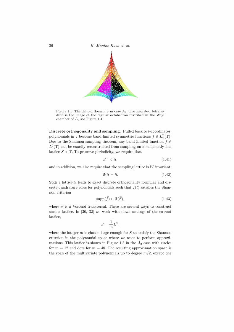
Figure 1.6 The deltoid domain δ in case A3. The inscribed tetrahe-dron is the image of the regular octahedron inscribed in the Weylchamber of 4, see Figure 1.4.
Discrete orthogonality and sampling. Pulled back to t-coordinates,
polynomials in z become band limited symmetric functions f ∈ L2∨(T).
Due to the Shannon sampling theorem, any band limited function f ∈L2(T) can be exactly reconstructed from sampling on a sufficiently fine
lattice S < T. To preserve periodicity, we require that
S⊥ < Λ, (1.41)
and in addition, we also require that the sampling lattice is W invariant,
WS = S. (1.42)
Such a lattice S leads to exact discrete orthogonality formulae and dis-
crete quadrature rules for polynomials such that f(t) satisfies the Shan-
non criterion
supp(f) ⊂ σ(S), (1.43)
where σ is a Voronoi transversal. There are several ways to construct
such a lattice. In [30, 32] we work with down scalings of the co-root
lattice,
S =1
mL∨,
where the integer m is chosen large enough for S to satisfy the Shannon
criterion in the polynomial space where we want to perform approxi-
mations. This lattice is shown in Figure 1.5 in the A2 case with circles
for m = 12 and dots for m = 48. The resulting approximation space is
the span of the multivariate polynomials up to degree m/2, except one

Through the Kaleidoscope 37
particular polynomial of degree m/2 which aliases to 0 on S. In addition
the space contains some particular polynomials of degree up to 23m.
Another lattice, which in many respects is more elegant, is the down-
scaling of the weights lattice
S =1
mΛ, for m ∈ N. (1.44)
With this discretization we obtain a perfect symmetry between primal
space and Fourier space. The primal space is the periodic domain T =
Rn/L∨, sampled in S = 1mΛ. The sampling turns the Fourier space into
the periodic domain Rn/S⊥ = Rn/mL∨. On the other hand, periodicity
under translation with L∨ in primal space is equivalent to sampling in
Fourier space at the lattice (L∨)⊥
= Λ. Thus, the discretized periodic
domain is self dual up to the scaling with m.
The sampling at S = 1mΛ is perfect also in the sense that we, for the
An Weyl groups, obtain an approximation space consisting of exactly
the n-variate polynomials up to degree m and nothing else. The space
of n-variate m-degree polynomials has dimension(m+nm
). The alcove 4
of the affine Weyl group An is a simplex with corners in the origin and
in λj , the principal dominant weights. Hence S is a downscaling of a
simplex containing(m+nm
)points, in particular these are the triangle
numbers for n = 2 and the pyramidal numbers for n = 3. In Fourier
space the situation is the same, the discrete space contains exactly the
n-variate Chebyshev polynomials of degree up to and including m.
Lebesgue numbers. The elegant sampling results above are useless
unless we can guarantee small Lebesque numbers and hence stable sam-
pling. Fortunately, the following result holds for the An family sampled
at the downscaled weights lattice.
Theorem 1.24 Let λ be the weights lattice in the affine Weyl group
An and let S = 1mΛ. Let z : 4 → δ be the coordinate change in (1.35).
The Lebesgue number of the points z(S) grows as
O(logn(m)). (1.45)
Similar results hold for other lattices (e.g. downscaled roots lattice)
and other affine Weyl groups. To prove this theorem, we must first show
that the Lagrangian interpolating polynomials in the nodal set z(S) are
given as
`j(z(t)) = c∑w∈W
DS(w(t− tj)) for all tj ∈ S,
38 H. Munthe-Kaas et. al.
where DS(t) is the polyhedral Dirichlet kernel. The result follows from
general bounds on Lebesgue numbers of the polyhedral Dirichlet ker-
nels [34, 36]. We omit the details. Similar results are shown for special
cases in [37].
Symmetric FFTs and fast Chebyshev expansions. In this para-
graph we let Φ be the root system An with Weyl group W ' Sn+1
with |W | = (n+ 1)!. Let S = 1mΛ and let G be the finite abelian group
G = S/L∨. Under the action of W on G, the fundamental domain is
4m = 4 ∪ S, where 4 is the n-simplex with corners in the origin and
in the fundamental dominant weights λj . Thus 4m consists of(m+nm
)points. The Weyl group also acts on G via the adjoint 〈ξ, wx〉 = 〈wξ, x〉,with fundamental domain 4m. Note that this case is self dual, so we
can identify 4m and 4m.
Let p(z) be a real n-variate polynomial of degree m and let f =
p(z(4m)) be the sampling of p(z). The Fourier transform is defined as
f(λ) = FG(πW∨ f)(λ) for λ ∈ 4m. (1.46)
The Chebyshev expansion of p(z) is
p(z) =∑λ∈4m
f(λ)Tλ(z). (1.47)
How fast can this Chebyshev expansion be computed? One possibility
is to extend f to CG and apply an FFT here. The number of points in
G is approximately N ≈ (n + 1)!(m+nm
). Counting both multiplications
and additions, a complex FFT on N points costs 5N log2(N) floating
point operations (flops).
It is, however, possible to improve the speed of this computation by
a factor 2|W | = 2(n + 1)! by using a symmetric FFT, as in [28]. The
factor 2 comes from the assumption that p(z) is real, not complex, and
the factor (n+1)! by carefully exploiting all the symmetries. This can be
implemented as a Cooley–Tukey style FFT computation. Letting m = 2k
we have a sequence of sub-lattices
S1 < S2 < S4 < · · · < S2k = Sm.
We know that Cooley–Tukey can be formulated with respect to arbi-
trary decompositions in sub-lattices. All the sub-lattices preserve all the
symmetries ofW , thus by organizing the computations carefully, it is suf-
ficient to compute in the fundamental domains of the action of W . How-
ever, the Cooley–Tukey splitting is not just a splitting in sub-lattices, it
Through the Kaleidoscope 39
also involves computations in the cosets of the sub-lattices. The cosets
may lose some symmetries of W , and for such cosets the fundamental
domain becomes larger. However, in that case the lost symmetry will
map one coset to another coset, and we may discard the cosets that
are equivalent to some other coset by a symmetry. In the dual space G,
the situation is similar, W acts by the adjoint action and we can simi-
larly exploit all the symmetries. In addition we have the real symmetry
expressed as f(λ) = f(−λ).
To make a rather complicated story short, by carefully paying atten-
tion to exploiting all the symmetries, it can be shown:
Theorem 1.25 Let πnm be the space of n-variate real polynomials of de-
gree m, a real vector space of dimension N =(m+nm
). The An Chebyshev
expansion of p(z) ∈ πnm can be computed in a stable manner by sampling
p(z) in the N points z(4m). The cost of this computation is 52N log2(N)
floating point numbers, counting both additions and multiplications.
Recurrence formulae. Practical computations with Chebyshev ex-
pansions rely on the availability of fast transforms between ‘nodal’ and
‘modal’ representation, i.e. between sampled values and Chebyshev ex-
pansion coefficients. Products of polynomials can be computed fast in
the nodal domain, while other operations such as integration and deriva-
tion can be done fast in the modal domain. Also, in the multivariate case,
there exist recursion formulae similar to the univariate case.
From the convolution product in EW∨ , one finds that the Tλ satisfy the
recurrence relations
T0 = 1, (1.48)
Tλj = zj , (1.49)
Tλ = Twλ for w ∈W, (1.50)
T−λ = Tλ, (1.51)
TλTµ =1
|W |∑w∈W
Tλ+wµ. (1.52)
These reduce to classical three-term recurrences for A1 and four term
recurrences for A2, see [30].
There also exist linear recurrence relations which compute the Cheby-
shev expansion of ∇p(z) from the Chebyshev expansion of p(z), see [32].
40 H. Munthe-Kaas et. al.
1.4 Conclusions
We have discussed various aspects of group theory as a tool for analyz-
ing numerical algorithms and for developing new computational algo-
rithms. In particular, we have focused on algorithms related to sampling
in regular lattices and algorithms related to applications of reflection
groups and kaleidoscopes. Group theory provides an important concep-
tual framework both for understanding the fundamental structure of
the algorithms and also for structuring the implementation of numerical
software.
Connections between group theory and Chebyshev approximations
have been discussed in detail. This is a connection which goes much
deeper than what has been presented in this paper. Weyl’s character
formula for the irreducible characters on simple Lie groups is essentially
identical to the definition of second kind multivariate Chebyshev poly-
nomials. Chebyshev approximation theory is therefore intimately linked
to approximation theory on Lie groups.
Another topic, which has not been discussed in this paper, is the
application of group theory in the development of algorithms for com-
puting time evolution of dynamical systems. Lie group integrators are
general numerical methods built around Lie group actions on the phase
space of the dynamical system [23]. Lie group integrators rely upon ex-
act computations of operator exponentials. The interplay between Lie
group integrators for time evolution and Chebyshev based spectral el-
ement methods for spatial discretizations is an active area of research
where all these techniques come together.
References
[1] K. Ahlander, M. Haveraaen, and H. Munthe-Kaas. On the role of math-ematical abstractions for scientific computing. In R. F. Boisvert andP. T. P. Tang, editors, The Architecture of Scientific Software, volume 60of IFIP Advances in Information and Communication Technology, pages145–158. Citeseer, 2001.
[2] K. Ahlander and H. Munthe-Kaas. Applications of the generalizedFourier transform in numerical linear algebra. BIT Numerical Mathe-matics, 45(4):819–850, 2005.
[3] E. L. Allgower, K. Georg, R. Miranda, and J. Tausch. Numerical ex-ploitation of equivariance. Zeitschrift fur Angewandte Mathematik undMechanik, 78:185–201, 1998.

Through the Kaleidoscope 41
[4] L. Auslander. Lecture notes on nil-theta functions. Number 34. AmerMathematical Society, 1977.
[5] L. Auslander and R. Tolimieri. Is computing with the finite Fouriertransform pure or applied mathematics. Notices of the AMS, 1(6), 1979.
[6] R. J. Beerends. Chebyshev polynomials in several variables and the ra-dial part of the Laplace–Beltrami operator. Transactions of the AMS,328(2):779–814, 1991.
[7] A. Bossavit. Symmetry, groups, and boundary value poblems. a progres-sive introduction to noncommutative harmonic analysis of partial differ-ential equations in domains with geometrical symmetry. Comput. Meth-ods Appl. Mech. and Engrg., 56:167–215, 1986.
[8] D. Bump. Lie Groups. Springer Verlag, 2004.[9] S.H. Christiansen, H.Z. Munthe-Kaas, and B. Owren. Topics in structure-
preserving discretization. Acta Numerica, 20(1):1–119, 2011.[10] J.H. Conway, N.J.A. Sloane, and E. Bannai. Sphere packings, lattices,
and groups, volume 290. Springer Verlag, 1999.[11] C. C. Douglas and J. Mandel. Abstract theory for the domain reduction
method. Computing, 48:73–96, 1992.[12] M. Dubiner. Spectral methods on triangles and other domains. Journal
of Scientific Computing, 6(4):345–390, 1991.[13] R. Eier and R. Lidl. A class of orthogonal polynomials in k variables.
Math. Ann., 260:93–99, 1982.[14] K. Engo, A. Marthinsen, and H.Z. Munthe-Kaas. Diffman: An object-
oriented matlab toolbox for solving differential equations on manifolds.Applied numerical mathematics, 39(3-4):323–347, 2001.
[15] A. F. Fassler and E. Stiefel. Group theoretical methods and their appli-cations. Birkhauser, Boston, 1992.
[16] K. Georg and R. Miranda. Exploiting symmetry in solving linear equa-tions. In E. L. Allgower, K. Bohmer, and M. Golubisky, editors, Bifur-cation and Symmetry, volume 104 of ISNM, pages 157–168. Birkhauser,Basel, 1992.
[17] F. X. Giraldo and T. Warburton. A nodal triangle-based specral elementmethod for the shallow water equations on the sphere. J. of Comp.Physics, 2005.
[18] R. Hadani and A. Singer. Representation theoretic patterns in threedimensional cryo-electron microscopy i-the intrinsic reconstitution algo-rithm. Arxiv preprint arXiv:0910.3009. To appear in Annals of Mathe-matics., 2009.
[19] R. Hadani and A. Singer. Representation theoretic patterns in three-dimensional cryo-electron microscopy ii—the class averaging problem.Foundations of Computational Mathematics, pages 1–28, 2011.
[20] J.S. Hesthaven and T. Warburton. Nodal discontinuous Galerkin meth-ods: algorithms, analysis, and applications, volume 54. Springer-VerlagNew York Inc, 2008.
[21] M. E. Hoffman and W. D. Withers. Generalized Chebyshev polynomialsassociated with affine Weyl groups. Transactions of the AMS, 308(1):91–104, 1988.
42 H. Munthe-Kaas et. al.
[22] D. Huybrechs. On the Fourier extension of non-periodic functions. SIAMJ. Numer. Anal., 47(6):4326–4355, 2010.
[23] A. Iserles, H. Munthe-Kaas, S. P. Nørsett, and A. Zanna. Lie-groupmethods. In Acta numerica, 2000, volume 9 of Acta Numer., pages 215–365. Cambridge Univ. Press, Cambridge, 2000.
[24] G. James and M. Liebeck. Representations and Characters of Groups.Cambridge University Press, 2 edition, 2001. ISBN 052100392X.
[25] T. Koornwinder. Orthogonal polynomials in two variables which areeigenfunctions of two algebraically independent partial differential op-erators I–IV. Indiag. Math., 36:48–66 and 357–381, 1974.
[26] R. Lidl. Tchebyscheffpolynome in mehreren Variabelen. J. Reine Angew.Math, 273:178–198, 1975.
[27] J. S. Lomont. Applications of Finite Groups. Academic Press, New York,1959.
[28] H. Munthe-Kaas. Symmetric FFTs; a general approach. In Topics in lin-ear algebra for vector- and parallel computers, PhD thesis. NTNU, Trond-heim, Norway, 1989. Available at: http://hans.munthe-kaas.no.
[29] H. Munthe-Kaas and T. Sørevik. Multidimensional pseudo-spectral meth-ods on lattice grids. Applied Numerical Mathematics, 2011.
[30] H.Z. Munthe-Kaas. On group Fourier analysis and symmetry preservingdiscretizations of PDEs. Journal of Physics A: Mathematical and General,39:5563, 2006.
[31] W. Rudin. Fourier analysis on groups, volume 12. Wiley-Interscience,1990.
[32] B.N. Ryland and H.Z. Munthe-Kaas. On Multivariate Chebyshev Poly-nomials and Spectral Approximations on Triangles. In J. S. Hesthavenand E. M. Rønquist, editors, Spectral and High Order Methods for PartialDifferential Equations, volume 76 of Lecture Notes Comp. Sci. and Eng.,pages 19–41. Springer, 2011.
[33] J. P. Serre. Linear Representations of Finite Groups. Springer, 1977.ISBN 0387901906.
[34] R.J. Stanton and P.A. Tomas. Polyhedral summability of Fourier serieson compact Lie groups. American Journal of Mathematics, 100(3):477–493, 1978.
[35] S. Thangavelu. Harmonic analysis on the Heisenberg group, volume 159.Birkhauser, 1998.
[36] G. Travaglini. Polyhedral summability of multiple Fourier series. InColloq. Math, volume 65, pages 103–116, 1993.
[37] Y. Xu. Fourier series and approximation on hexagonal and triangulardomains. Constructive Approximation, 31(1):115–138, 2010.


![Kaleidoscope - Amazon Web Services€¦ · Kaleidoscope Make your own reflecting kaleidoscope Written By: Kailash NR Kaleidoscope Guide ID: 520 -Release: 1.0 [major] 2019-02-04 This](https://cdn.vdocuments.mx/doc/165x107/5fa4c91eb608da22fd275ca1/kaleidoscope-amazon-web-services-kaleidoscope-make-your-own-reflecting-kaleidoscope.jpg)
