
1
THE NORMAL DISTRIBUTION
In the analysis so far, we have discussed the mean and the variance of a distribution of a random variable, but we have not said anything specific about the actual shape of the distribution. It is time to do that.
00 m
f(X)
X

2
There are only four distributions, all of them continuous, that are going to be of importance to us: the normal distribution, the t distribution, the F distribution, and the chi-squared (2) distribution.
THE NORMAL DISTRIBUTION
00 m
f(X)
X

3
The normal distribution has the graceful, bell-shaped form shown.
THE NORMAL DISTRIBUTION
00 m
f(X)
X

4
The probability density function for a normally distributed random variable X is as shown,where and are parameters.
THE NORMAL DISTRIBUTION
00 m
f(X)
X
2
21
21
X
eXf

5
It is in fact an infinite family of distributions since can be any finite real number and any finite positive real number.
THE NORMAL DISTRIBUTION
00 m
f(X)
X
2
21
21
X
eXf
6
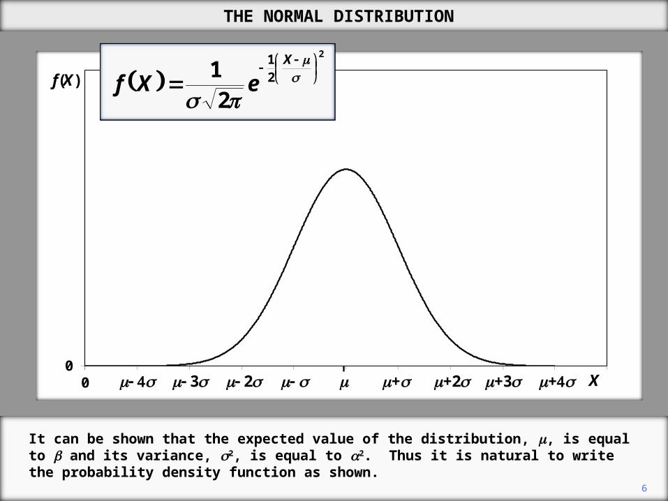
It can be shown that the expected value of the distribution, m, is equal to and its variance, 2, is equal to 2. Thus it is natural to write the probability density function as shown.
THE NORMAL DISTRIBUTION
00 m X
f(X)
m+ m+2 m+3m 3 m m 2m 4 m+4
2
21
21
m
X
eXf

7
The distribution is symmetric, so it automatically follows that the mean and the mode coincide in the middle of the distribution.
THE NORMAL DISTRIBUTION
00 m X
f(X)
m+ m+2 m+3m 3 m m 2m 4 m+4
2
21
21
m
X
eXf

8
The shape of the distribution is fixed when expressed in terms of standard deviations, so all normal distributions look the same when expressed in terms of m and . This is shown in figure.
THE NORMAL DISTRIBUTION
00 m X
f(X)
m+ m+2 m+3m 3 m m 2m 4 m+4
2
21
21
m
X
eXf

9
As a matter of mathematical shorthand, if a variable X is normally distributed with mean m and variance 2, this is written X ~ N(m, 2). (The symbol ~ means ‘is distributed as’). The first argument in the parentheses refers to the mean and the second to the variance.
THE NORMAL DISTRIBUTION
00 m X
f(X)
m+ m+2 m+3m 3 m m 2m 4 m+4
2
21
21
m
X
eXf
2,~ mNX

10
This, of course, is the general expression. If you had a specific normal distribution, you would replace the arguments with the actual numerical values.
THE NORMAL DISTRIBUTION
00 m X
f(X)
m+ m+2 m+3m 3 m m 2m 4 m+4
2
21
21
m
X
eXf
2,~ mNX
11
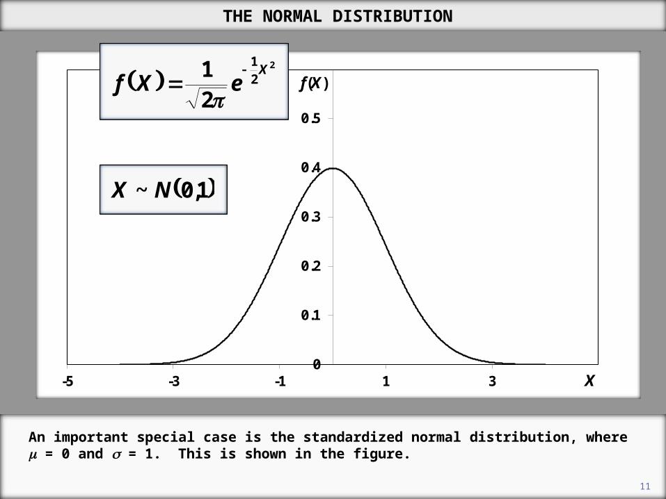
An important special case is the standardized normal distribution, where m = 0 and = 1. This is shown in the figure.
THE NORMAL DISTRIBUTION
0
0.1
0.2
0.3
0.4
0.5
-5 -3 -1 1 3 X
f(X) 2
21
21 XeXf
1,0~ NX

Copyright Christopher Dougherty 2012.
These slideshows may be downloaded by anyone, anywhere for personal use.
Subject to respect for copyright and, where appropriate, attribution, they may be
used as a resource for teaching an econometrics course. There is no need to
refer to the author.
The content of this slideshow comes from Section R.8 of C. Dougherty,
Introduction to Econometrics, fourth edition 2011, Oxford University Press.
Additional (free) resources for both students and instructors may be
downloaded from the OUP Online Resource Centre
http://www.oup.com/uk/orc/bin/9780199567089/.
Individuals studying econometrics on their own who feel that they might benefit
from participation in a formal course should consider the London School of
Economics summer school course
EC212 Introduction to Econometrics
http://www2.lse.ac.uk/study/summerSchools/summerSchool/Home.aspx
or the University of London International Programmes distance learning course
EC2020 Elements of Econometrics
www.londoninternational.ac.uk/lse.
2012.10.31


