Download - 1 Seasonal Adjustments: Causes of Revisions Øyvind Langsrud Statistics Norway [email protected]

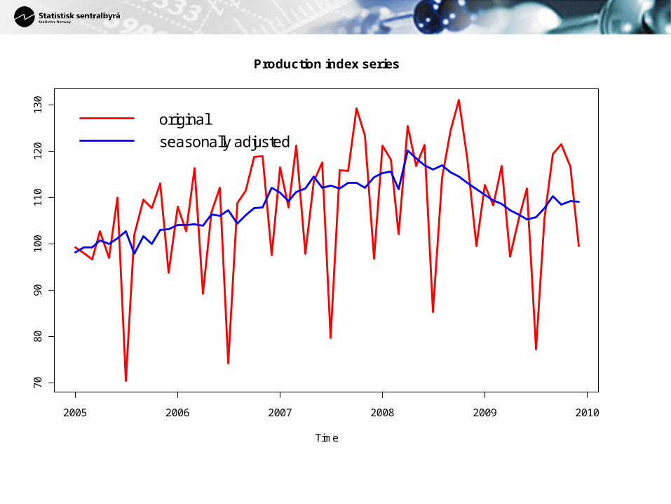
Production index series
Time
2005 2006 2007 2008 2009 2010
70
80
90
10
01
10
12
01
30
original
seasonally adjusted

Seasonally adjustment based on
X12-ARIMA• Two-step procedure: regARIMA + trend and seasonal filters
• regARIMA – Seasonal ARIMA model with regression parameters – Holiday and trading day adjustment– Produce forecasts for use in the next step
• Important choices– Type of ARIMA model– Regression parameters: Holidays and trading days– How to handle outliers
langsrud_pdf_movie.pdf

Revision
• The revision is caused by updated models and parameters
• Revision is a problem– Can be confusing– Not easy to communicate
• Choosing seasonal adjustment methodology can be viewed as a question of balancing
– the requirement of optimal seasonal adjustment at each time point– against the requirement of minimal revisions.
• Can revision be reduced without reducing the quality of the adjustment?

Revision on log-scale
• At = seasonally adjusted series. Yt = original series
• At|t+h is the seasonal adjustment of Yt calculated from the series
where Yt+h is the last observation
• OneMonthRevisiont = (log(At|t+1) – log(At|t) )*100%

one-month revisions
Time
Pe
rce
nt
2005 2006 2007 2008 2009 2010
-1.5
-1.0
-0.5
0.0
0.5
1.0
1.5
Final seasonally adjusted data (d11)
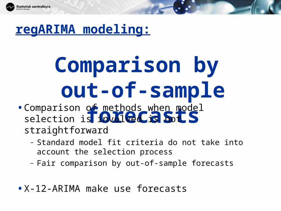
regARIMA modeling:
Comparison by out-of-sample forecasts
• Comparison of methods when model selection is involved is not straightforward
– Standard model fit criteria do not take into account the selection process
– Fair comparison by out-of-sample forecasts
• X-12-ARIMA make use forecasts

Relative forecasting error
• Yt+h|t is the forecast of Yt+h calculated from the series where
Yt is the last observation
• Example: Yt+h|t =101, Yt+h =100– 100% * (101-100)/101 = 0.99099%– 100% * (log(101)-log(100)) = 0.995033%– 100% * (101-100)/100 = 1.00000%

% opposite log- increase denominator based
0.01 0.009999 0.01000 0.10 0.099900 0.09995 1.00 0.990099 0.99503 2.00 1.960784 1.98026 5.00 4.761905 4.87902 10.00 9.090909 9.53102 20.00 16.666667 18.23216 50.00 33.333333 40.54651 100.00 50.000000 69.31472
Other examples

% opposite log- increase denominator based
0.01 0.009999 0.01000 0.10 0.099900 0.09995 1.00 0.990099 0.99503 2.00 1.960784 1.98026 5.00 4.761905 4.87902 10.00 9.090909 9.53102 20.00 16.666667 18.23216 50.00 33.333333 40.54651 100.00 50.000000 69.31472
Other examples

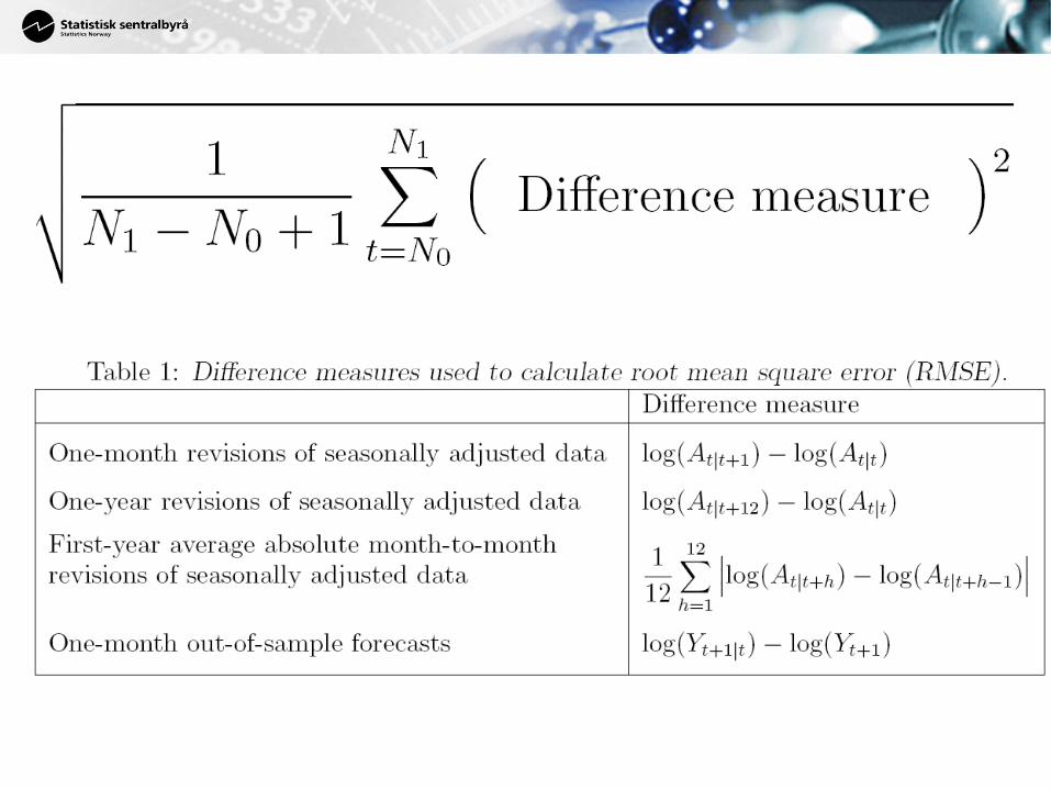
RMSEroot mean square error

RMSEroot mean square error
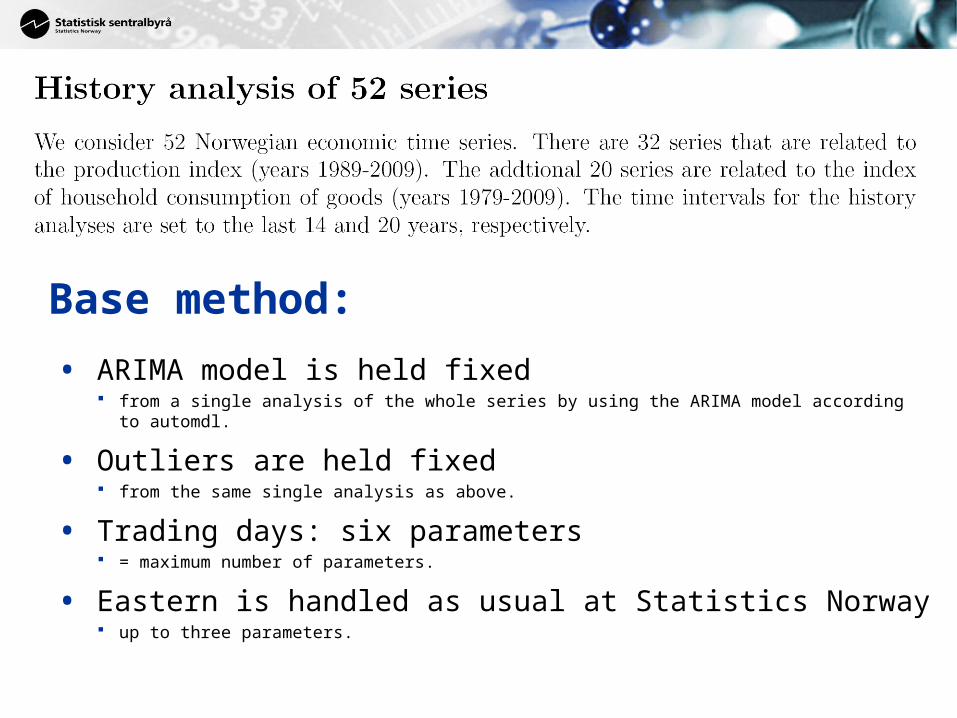
• ARIMA model is held fixed from a single analysis of the whole series by using the ARIMA model according to automdl.
• Outliers are held fixed from the same single analysis as above.
• Trading days: six parameters = maximum number of parameters.
• Eastern is handled as usual at Statistics Norway up to three parameters.
Base method:

• ARIMA model is held fixed from a single analysis of the whole series by using the ARIMA model according to automdl.
• Outliers are held fixed from the same single analysis as above.
• Trading days: six parameters = maximum number of parameters.
• Eastern is handled as usual at Statistics Norway up to three parameters.
Comparing methods by deviating from the base method

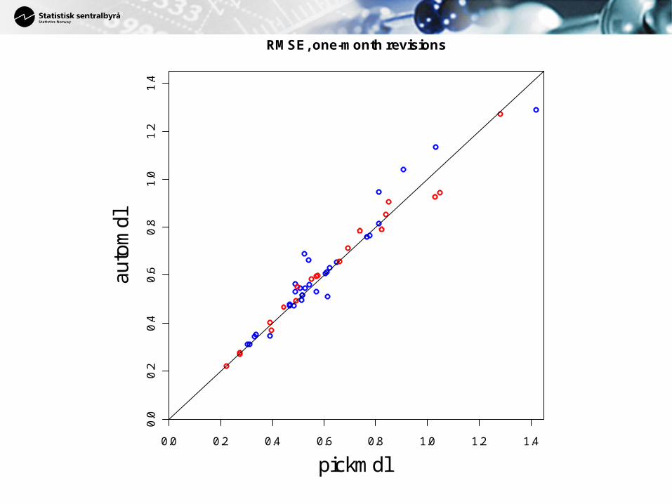
Automatic ARIMA model selection:
automdl vs pickmdl
• automdl as default in X-12-ARIMA
• pickmdl selects ARIMA model from five candidates
(0 1 1)(0 1 1) *(0 1 2)(0 1 1) X(2 1 0)(0 1 1) X(0 2 2)(0 1 1) X(2 1 2)(0 1 1) X

0 1 2 3 4 5
01
23
45
RMSE, one-month revisions
pickmdl
auto
mdl
Production indexIndex of household consumption of goods

0.0 0.2 0.4 0.6 0.8 1.0 1.2 1.4
0.0
0.2
0.4
0.6
0.8
1.0
1.2
1.4
RMSE, one-month revisions
pickmdl
auto
mdl
Production indexIndex of household consumption of goods
0.0 0.2 0.4 0.6 0.8 1.0 1.2 1.4
0.0
0.2
0.4
0.6
0.8
1.0
1.2
1.4
RMSE, one-month revisions
pickmdl
auto
mdl

0.0 0.5 1.0 1.5 2.0 2.5
0.0
0.5
1.0
1.5
2.0
2.5
RMSE, one-year revisions
pickmdl
auto
mdl

0.0 0.1 0.2 0.3 0.4 0.5
0.0
0.1
0.2
0.3
0.4
0.5
RMSE, first-year average absolute month-to-month revisions
pickmdl
auto
mdl

0 2 4 6 8 10 12
02
46
81
01
2
RMSE, one-month out-of-sample forecasts
pickmdl
auto
mdl

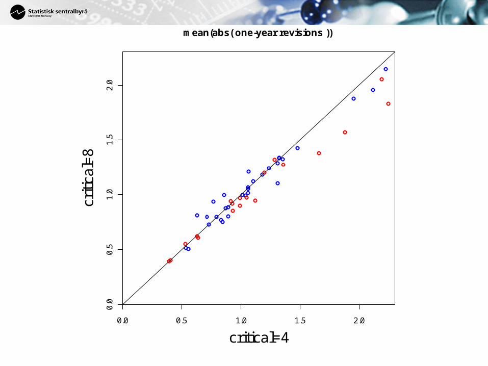
Automatic outlier detection:
critical=4 vs critical=8
• t-statistic limit
• Both additive outliers and level shifts
• Critical=4 is close to default in X-12-ARIMA
• Critical=8: outliers are extremely rare

0.0 0.5 1.0 1.5 2.0
0.0
0.5
1.0
1.5
2.0
RMSE, one-month revisions
critical=4
criti
cal=
8

0.0 0.2 0.4 0.6 0.8 1.0 1.2
0.0
0.2
0.4
0.6
0.8
1.0
1.2
mean(abs( one-month revisions ))
critical=4
criti
cal=
8

0.0 0.5 1.0 1.5 2.0 2.5 3.0
0.0
0.5
1.0
1.5
2.0
2.5
3.0
RMSE, one-year revisions
critical=4
criti
cal=
8
0.0 0.5 1.0 1.5 2.0
0.0
0.5
1.0
1.5
2.0
mean(abs( one-year revisions ))
critical=4
criti
cal=
8

0.0 0.2 0.4 0.6 0.8
0.0
0.2
0.4
0.6
0.8
RMSE, first-year average absolute month-to-month revisions
critical=4
criti
cal=
8

0.0 0.1 0.2 0.3 0.4 0.5 0.6 0.7
0.0
0.1
0.2
0.3
0.4
0.5
0.6
0.7
mean(abs( first-year average absolute month-to-month revisions ))
critical=4
criti
cal=
8

0 2 4 6 8 10 12
02
46
81
01
2
RMSE, one-month out-of-sample forecasts
critical=4
criti
cal=
8

0 2 4 6 8
02
46
8
mean(abs( one-month out-of-sample forecasts ))
critical=4
criti
cal=
8
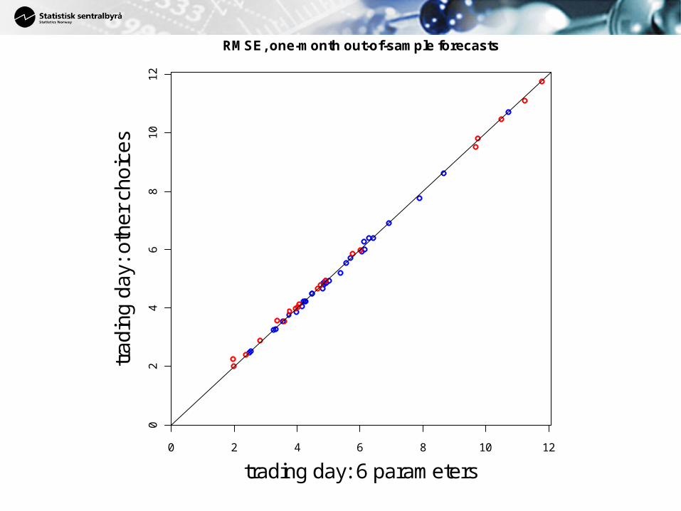
Trading day:6 parameters vs other choices
• 6 parameters = maximum number of parameters
• Other choices – Production index– Standard choice at Statistics Norway based on industrial knowledge – 0, 1, 5 and 6 parameters
• Other choices – Index of household consumption of goods
– 1 parameter, weekdays vs Sundays/Saturdays

0.0 0.2 0.4 0.6 0.8 1.0 1.2 1.4
0.0
0.2
0.4
0.6
0.8
1.0
1.2
1.4
RMSE, one-month revisions
trading day: 6 parameters
trad
ing
day:
oth
er c
hoic
es

0.0 0.5 1.0 1.5 2.0 2.5
0.0
0.5
1.0
1.5
2.0
2.5
RMSE, one-year revisions
trading day: 6 parameters
trad
ing
day:
oth
er c
hoic
es

0.0 0.1 0.2 0.3 0.4 0.5
0.0
0.1
0.2
0.3
0.4
0.5
RMSE, first-year average absolute month-to-month revisions
trading day: 6 parameters
trad
ing
day:
oth
er c
hoic
es
0 2 4 6 8 10 12
02
46
81
01
2
RMSE, one-month out-of-sample forecasts
trading day: 6 parameters
trad
ing
day:
oth
er c
hoic
es

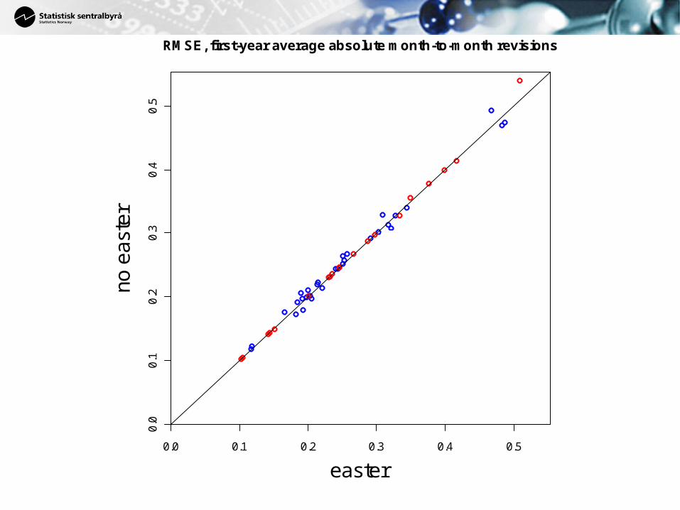
Moving holiday:
Easter vs no Easter
• Method in Norway– Up to three parameters: Before Easter, Easter, After Easter– Selection based on model fit an t-tests
• History analysis– Exactly as today’s Norwegian procedure

0.0 0.2 0.4 0.6 0.8 1.0 1.2
0.0
0.2
0.4
0.6
0.8
1.0
1.2
RMSE, one-month revisions
easter
no e
aste
r

0.0 0.5 1.0 1.5 2.0 2.5 3.0
0.0
0.5
1.0
1.5
2.0
2.5
3.0
RMSE, one-year revisions
easter
no e
aste
r
0.0 0.1 0.2 0.3 0.4 0.5
0.0
0.1
0.2
0.3
0.4
0.5
RMSE, first-year average absolute month-to-month revisions
easter
no e
aste
r

0 2 4 6 8 10 12
02
46
81
01
2
RMSE, one-month out-of-sample forecasts
easter
no e
aste
r

Conclusion
• Automatic outlier detection and ARIMA model selection leads to revision problems
– Problems can be reduced by using pickmdl and by increasing outlier detection limit
– Better solutions by fixing outliers and models
• Holidays and trading days are less important– Norway’s procedure may be improved– More investigation will be performed

Findley DF (2005),"Some Recent Developments and Directions in Seasonal",JOURNAL OF OFFICIAL STATISTICS, Vol 21, 343–365
Findley DF, Monsell BC, Bell WR, Otto MC, and Chen BC (1998),"New capabilities and methods of the X-12-ARIMA seasonal-adjustment program",JOURNAL OF BUSINESS & ECONOMIC STATISTICS, Vol. 16, 127-152.
Roberts CG, Holan SH, Monsell B (2010),"Comparison of X-12-ARIMA Trading Day and Holiday Regressors with Country Specific
Regressors",JOURNAL OF OFFICIAL STATISTICS, Vol 26, 371-394
US Census Bureau (2011),"X-12-ARIMA Reference Manual",http://www.census.gov/ts/x12a/v03/x12adocV03.pdf
UK - The Office for National Statistics (2007),"Guide to Seasonal Adjustment with X-12-ARIMA **DRAFT**",http://www.ons.gov.uk/ons/guide-method/method-quality/general-methodology/time-series-analysis/guide-to-seasonal-adjustment.pdf
Eurostat - Methodologies and working papers (2009)"Ess Guidelines on Seasonal Adjustment",http://epp.eurostat.ec.europa.eu/cache/ITY_OFFPUB/KS-RA-09-006/EN/KS-RA-09-006-EN.PDF

X12-ARIMA output series
d11 = Y/e18, in our modelleing e18 = e10*d18Y = Original series
d11 = Final seasonally adjusted data (At)
e18 = Final adjustment ratios
d10 = Final seasonal factors
d18 = Combined holiday and trading day factors
• Can calculate revisions in e18, d10, d18 similar to d11d11revision = - e18revision
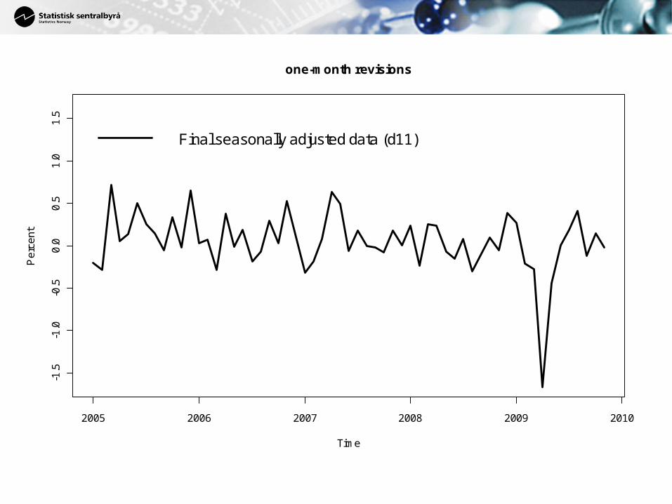
one-month revisions
Time
Pe
rce
nt
2005 2006 2007 2008 2009 2010
-1.5
-1.0
-0.5
0.0
0.5
1.0
1.5
Final seasonally adjusted data (d11)

one-month revisions
Time
2005 2006 2007 2008 2009 2010
-1.5
-1.0
-0.5
0.0
0.5
1.0
1.5 Final adjustment ratios (e18)
Final seasonally adjusted data (d11)

one-month revisions
Time
Pe
rce
nt
2005 2006 2007 2008 2009 2010
-1.5
-1.0
-0.5
0.0
0.5
1.0
1.5 Final adjustment ratios (e18)

one-month revisions
Time
2005 2006 2007 2008 2009 2010
-1.5
-1.0
-0.5
0.0
0.5
1.0
1.5 Final adjustment ratios (e18)
Final seasonal factors (d10)
Combined holiday and trading day factors (d18)


