
1
Queuing AnalysisOverview
• What is queuing analysis?- to study how people behave in waiting in line so that we
could provide a solution with minimizing waiting time and resources allocation
Two elements involved in waiting lines (to p2)
2
Two elements involved in waiting lines
1. Arrival rate, • Rate of people joining to the queue
2. Service rate, • Rate of service that service provided
How do they applied in a real life? (to p3)

3
Queuing Analysis
(p9)
Service rate,
Arrival rate,
This phenomenon is known as Single-server Waiting Line
How to study it? (to p4)
4
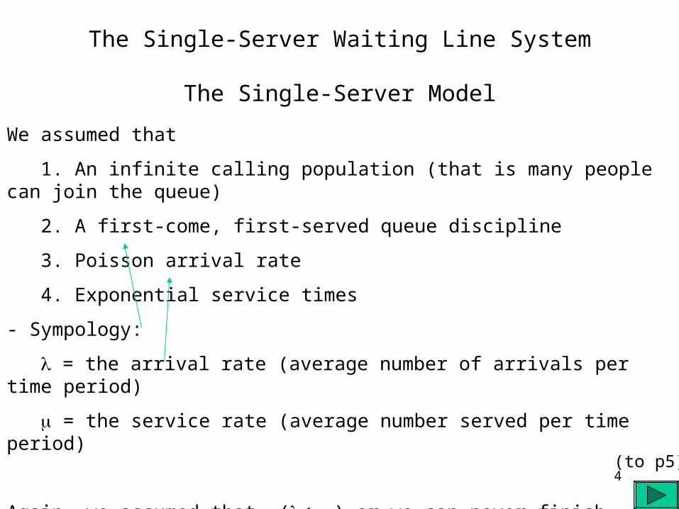
The Single-Server Waiting Line System
The Single-Server Model
We assumed that
1. An infinite calling population (that is many people can join the queue)
2. A first-come, first-served queue discipline
3. Poisson arrival rate
4. Exponential service times
- Sympology:
= the arrival rate (average number of arrivals per time period)
= the service rate (average number served per time period)
Again, we assumed that (< ) or we can never finish service customers before the end of the day! (to p5)

5
The relationship between and • We adopted a “birth-and-death” process to
study their relationship
And we have the following results:P0 = Prob that no one in the queue
Ls= number people waiting in the system
Lq=number people waiting in the queue
Ws= total waiting time in the system
Wq= total waiting time in the queue
How these L, W values are represented
(to p18)
(to p6)
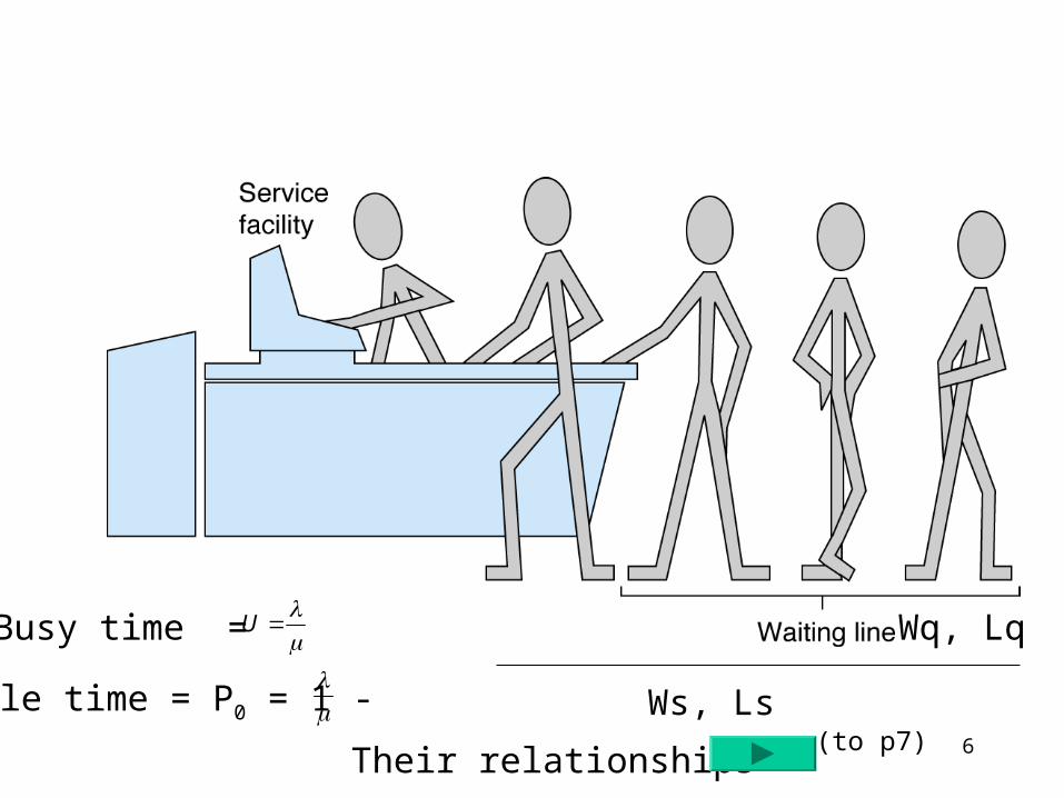
6
Wq, Lq
Ws, Ls
Busy time =
U
Idle time = P0 = 1 -
Their relationships (to p7)

7
The Single-Server Waiting Line SystemBasic Single-Server Queuing Formulas
Probability that no customers are in the queuing system:
Probability that n customers are in the system:
Average number of customers in system: and waiting line:
Average time customer spends waiting and being served:
Average time customer spends waiting in the queue:
Probability that server is busy (utilization factor):
Probability that server is idle:
11oP
11 n
n
o
n
n PP
LLq
2
LW11
LWq
1
U
11 UI
L
Note: the process to derive these formulasare based on the “birth-and-death” process
Example(to p8)
8
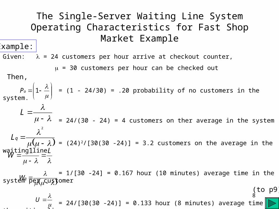
The Single-Server Waiting Line SystemOperating Characteristics for Fast Shop Market Example
Given: = 24 customers per hour arrive at checkout counter,
= 30 customers per hour can be checked out
= (1 - 24/30) = .20 probability of no customers in the system.
= 24/(30 - 24) = 4 customers on ther average in the system
= (24)2/[30(30 -24)] = 3.2 customers on the average in the waiting line
= 1/[30 -24] = 0.167 hour (10 minutes) average time in the system per customer
= 24/[30(30 -24)] = 0.133 hour (8 minutes) average time in the waiting line
= 24/30 = .80 probability server busy, .20 probability server will be idle
1oP
L
2
qL
L
W
1
qW
U
Example:
Then,
(to p9)

9
The Single-Server Waiting Line System
Steady-State Operating Characteristics
Because of steady -state nature of operating characteristics:
- Utilization factor, U, must be less than one: U<1,or / <1 and < .
- The ratio of the arrival rate to the service rate must be less than one
or, the service rate must be greater than the arrival rate.
- The server must be able to serve customers faster than the arrival rate in the long run, or waiting line will grow to infinite size.
What if Utilization rate >= 1? (what would happened?)
Changing of the values of , .
Important note:
(to p10)

10
• Consider another case where,
– Manager wishes to test several alternatives for reducing customer waiting time:
• 1. Addition of another employee to pack up purchases
• 2. Addition of another checkout counter.
– Which one of the three models that we should deploy?
• Answer:
– Comparing its operating characteristics
• (all three examples with calculation) (to p13)
(to p11)
(to p12)

11
The Single-Server Waiting Line SystemEffect of Operating Characteristics on Managerial Decisions
(1 of 3)
- Alternative 1: Addition of an employee (raises service rate from = 30 to = 40 customers per hour)
Cost $150 per week, avoids loss of $75 per week for each minute of reduced customer waiting time.
System operating characteristics with new parameters:
Po = .40 probability of no customers in the system
L = 1.5 customers on the average in the queuing system
Lq = 0.90 customer on the average in the waiting line
W = 0.063 hour (3.75 minutes) average time in the system per customer
Wq = 0.038 hour ( 2.25 minutes) average time in the waiting line per customer
U = .60 probability that server is busy and customer must wait, .40 probability server available
Average customer waiting time reduced from 8 to 2.25 minutes worth $431.25 per week.
Net savings = $431.25 - 150 = $281.25 per week.
= 1 - (24/40)
i.e. (5.75*$75)
(to p10)

12
The Single-Server Waiting Line SystemEffect of Operating Characteristics on Managerial Decisions
(2 of 3)- Alternative 2: Addition of a new checkout counter ($6,000 plus $200 per week for additional cashier)
=24/2 = 12 customers per hour per checkout counter.
= 30 customers per hour at each counter
System operating chacteristics with new parameters:
Po = .60 probability of no customers in the system
L = 0.67 customer in the queuing system
Lq = 0.27 customer in the waiting line
W = 0.055 hour (3.33 minutes) per customer in the system
Wq = 0.022 hour (1.33 minutes) per customer in the waiting line
U = .40 probability that a customer must wait
I = .60 probability that server is idle and customer can be served.
Savings from reduced waiting time worth $500 per week - $200 = $300 net savings per week.
After $6,000 recovered, alternative 2 would provide $300 -281.25 = $18.75 more savings per week.
(to p10)

13
The Single-Server Waiting Line SystemEffect of Operating Characteristics on Managerial Decisions
(3 of 3)
Table 13.1Operating Characteristics for Each Alternative System
Figure 13.2Cost trade-offs for service
levels
Decision: very much dependedon manager’s experience because there is difficult to obtain “the”best solution ..
Note: Min cost is not obtained here
(to p14)

14
One last note
• The Single waiting line system we studied here can be denoted as: (to p15)
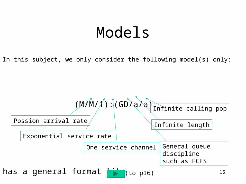
15
Models
In this subject, we only consider the following model(s) only:
(M/M/1):(GD/a/a)
Possion arrival rate
Exponential service rate
One service channel General queue disciplinesuch as FCFS
Infinite length
Infinite calling pop
It has a general format like (to p16)

16
Type of models
(A/B/C): (D/E/F)
Number of channels(parallel servers)
Arrival distribution
Service distribution Queue capacity,such max ppl in the queue length
Queue discipline, such as FCFS
Size of population
Tutorial Questions (to p17)
Example: M/M/S with finite population
17
Tutorial Questions
• Ex: 7, 8, 9 and 12
(END)
End

18

19
The Single-Server Waiting Line SystemOperating Characteristics for Fast Shop Market Example
Given: = 24 = 24 = 24 /2=12
= 30 = 40 = 30
= (1 - 24/30) = .20 1-24/40 =0.4 1-12/30=0.6
= 24/(30 - 24) = 4 1.5 0.67
= (24)2/[30(30 -24)] = 3.2 0.9 0.27
= 1/[30 -24] = 0.167 hour (10 minutes) 0.063(3.75 mins) 0.055(3.33min)
= 24/[30(30 -24)] = 0.133 hour (8 minutes) 0.038 (2.25 min) 0.022 (1.33 min)
= 24/30 = .80 probability server busy, .20 0.6 0.4
1oP
L
2
qL
L
W
1
qW
U
Example:1
Then,
(to p9)
Alternative 1 Alternative 2

![15-744: Computer Networking L-5 Fair Queuing. 2 Fair Queuing Core-stateless Fair queuing Assigned reading [DKS90] Analysis and Simulation of a Fair Queueing](https://cdn.vdocuments.mx/doc/165x107/56649dc65503460f94abad7b/15-744-computer-networking-l-5-fair-queuing-2-fair-queuing-core-stateless.jpg)


