
1
Automatic Text Classification
Yutaka Sasaki
NaCTeM
School of Computer Science
©2007 Yutaka Sasaki, University of Manchester

2
Introduction
©2007 Yutaka Sasaki, University of Manchester

3
Introduction
• Text Classification is the task:– to classify documents into predefined classes
• Text Classification is also called– Text Categorization– Document Classification– Document Categorization
• Two approaches– manual classification and automatic classification
©2007 Yutaka Sasaki, University of Manchester

4
Relevant technologies• Text Clustering
– Create clusters of documents without any external information
• Information Retrieval (IR)– Retrieve a set of documents relevant to a query
• Information Filtering– Filter out irrelevant documents through interactions
• Information Extraction (IE)– Extract fragments of information, e.g., person names, dates, and
places, in documents
• Text Classification– No query, interactions, external information– Decide topics of documents
©2007 Yutaka Sasaki, University of Manchester

5
Examples of relevant technologies
©2007 Yutaka Sasaki, University of Manchester
web documents

6
Example of clustering
web documents
©2007 Yutaka Sasaki, University of Manchester

7
Examples of information retrieval
x
web documents
©2007 Yutaka Sasaki, University of Manchester

8
Examples of information filtering
web documents
©2007 Yutaka Sasaki, University of Manchester

9
Examples of information extraction
web documents about accidents
Date: 04/12/03Place: LondonType: trafficCasualty: 5
Key information on accidents
©2007 Yutaka Sasaki, University of Manchester
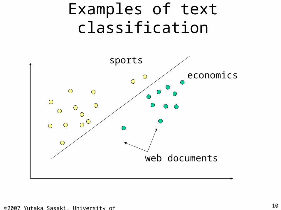
10
Examples of text classification
web documents
©2007 Yutaka Sasaki, University of Manchester
sports
economics

11
Text Classification Applications
• E-mail spam filtering• Categorize newspaper articles and newswires into
topics• Organize Web pages into hierarchical categories• Sort journals and abstracts by subject categories
(e.g., MEDLINE, etc.)• Assigning international clinical codes to patient
clinical records
©2007 Yutaka Sasaki, University of Manchester

12
Simple text classification example
• You want to classify documents into 4 classes:
economics, sports, science, life.
• There are two approaches that you can take:– rule-based approach
• write a set of rules that classify documents
– machine learning-based approach• using a set of sample documents that are classified into
the classes (training data), automatically create classifiers based on the training data
©2007 Yutaka Sasaki, University of Manchester

13
Comparison of Two Approaches (1)
Rule-based classification Pros:
– very accurate when rules are written by experts– classification criteria can be easily controlled when the
number of rules are small.
Cons:– sometimes, rules conflicts each other
• maintenance of rules becomes more difficult as the number of rules increases
– the rules have to be reconstructed when a target domain changes
– low coverage because of a wide variety of expressions
©2007 Yutaka Sasaki, University of Manchester

14
Comparison of Two Approaches (2)
Machine Learning-based approach
Pros:– domain independent
– high predictive performance
Cons:– not accountable for classification results
– training data required
©2007 Yutaka Sasaki, University of Manchester

15
Formal Definition
• Given:– A set of documents D = {d1, d2,…, dm}
– A fixed set of topics T = {t1, t2,…, tn}
• Determine:– The topic of d: t(d) T, where t(x) is a
classification function whose domain is D and whose range is T.
©2007 Yutaka Sasaki, University of Manchester

16
Rule-based approachExample: Classify documents into sports
“ball” must be a word that is frequently used in sports
Rule 1: “ball” d t(d) = sports
But there are other meanings of “ball”Def.2-1 : a large formal gathering for social dancing (WEBSTER)
Rule 2: “ball” d & “dance” d t(d) = sports
Def.2-2 : a very pleasant experience : a good time (WEBSTER)
Rule 3: “ball” d & “dance” d & “game” d &
“play” d t(d) = sports
Natural language has a rich variety of expressions:
e.g., “Many people have a ball when they play a bingo game.”
©2007 Yutaka Sasaki, University of Manchester

17
Machine Learning Approach1.Prepare a set of training data
• Attach topic information to the documents in a target domain.
2.Create a classifier (model) • Apply a Machine Learning tool to the data
• Support Vector Machine (SVM), Maximum Entropy Models (MEM)
3.Classify new documents by the classifier
sports
science
lifeclassifier
sports
science
lifeclassifier
…
life
sports
Training data
©2007 Yutaka Sasaki, University of Manchester

18
Closer look atMachine Learning-based approach
f1
f2
f3
f4
game
play
ball
danceClassifier c(·|·)
c(sports|x)
document d
c(science|x)
c(economics|x)
c(y|x)
x=(f1, f2, f3, f4)
features
feature extraction
feature vector(input vector) c(life|x)
Select the best classification result
©2007 Yutaka Sasaki, University of Manchester

19
Rule-based vs. Machine Learning-based[Creecy at al., 1992]
• Data: US Census Bureau Decennial Census 1990– 22 million natural language responses– 232 industry categories and 504 occupation categories– It costs about $15 million if fully done by hand
• Define classification rules manually:– Expert System AIOCS– Development time: 192 person-months (2 people, 8 years)– Accuracy = 57%(industry), 37%(occupation)
• Learn classification function– Machine Learning-based System PACE– Development time: 4 person-months– Accuracy = 63%(industry), 57%(occupation)
©2007 Yutaka Sasaki, University of Manchester

20
Evaluation
©2007 Yutaka Sasaki, University of Manchester

21
Common Evaluation Metrics
• Accuracy• Precision• Recall• F-measure
– harmonic mean of recall and precision– micro-average F1
• global calculation of F1 regardless of topics– macro-average F1:
• average on F1 scores of all the topics
©2007 Yutaka Sasaki, University of Manchester

22
Accuracy
• The rate of correctly predicted topics
system’s predictioncorrect answer
truepositive
false positive(Type I error, false alarm)
false negative(Type II error, missed alarm)
(TP) (FP)(FN)
Accuracy = TP + TN TP + FP + FN + TN
true negative(TN)
©2007 Yutaka Sasaki, University of Manchester

23
Accuracy• Example: classify docs into spam or not spam
Accuracy = = = 0.4 TP+TN TP+FP+FN+TN
d1
d2
d3
Y
Y
N
system’s prediction correct answer
N
Y
Y
TP FP FN TN
1
1
1
1
1
d4 N
1+1 1+2+1+1
N
d5 NY
©2007 Yutaka Sasaki, University of Manchester

24
Issue in Accuracy• When a certain topic (e.g., not-spam) is a majority, the
accuracy easily reaches a high percentage.
Accuracy = = = 0.99 TP+TN TP+FP+FN+TN
d1…
N
N
system’s prediction correct answer
Y
Y
TP FP FN TN
1
1
990d11-d1000
990 1000
N … N
d10
… … … …
N…N
©2007 Yutaka Sasaki, University of Manchester

25
Precision
• The rate of correctly predicted topics
system’s predictioncorrect answer
truepositive
false positive(Type I error, false alarm)
false negative(Type II error, missed alarm)
(TP) (FP)(FN)
Precision = TPTP + FP
true negative(TN)
©2007 Yutaka Sasaki, University of Manchester

26
Precision• Example: classify docs into spam or not spam
Precision = = = 0.333TPTP+FP
d1
d2
d3
Y
Y
N
system’s prediction correct answer
N
Y
Y
TP FP FN TN
1
1
1
1
1
d4 N
11+2
N
d5 NY
©2007 Yutaka Sasaki, University of Manchester

27
Issue in Precision• When a system outputs only confident topics, the
precision easily reaches a high percentage.
Accuracy = = = 1 TPTP+FP
d1…
N
N
system’s prediction correct answer
Y
N
TP FP FN TN
1
1
1
11
Y
d999
… …(Y or N)… … …
Yd1000
©2007 Yutaka Sasaki, University of Manchester

28
Recall
• The rate of correctly predicted topics
system’s predictioncorrect answer
truepositive
false positive(Type I error, false alarm)
false negative(Type II error, missed alarm)
(TP) (FP)(FN)
Precision = TPTP + FN
true negative(TN)
©2007 Yutaka Sasaki, University of Manchester

29
Recall• Example: classify docs into spam or not spam
Precision = = = 0.5 TPTP+FN
d1
d2
d3
Y
Y
N
system’s prediction correct answer
N
Y
Y
TP FP FN TN
1
1
1
1
1
d4 N
11+1
N
d5 NY
©2007 Yutaka Sasaki, University of Manchester

30
Issue in Recall• When a system outputs loosely, the recall easily
reaches a high percentage.
Accuracy = = = 1 TPTP+FN
d1…
Y
Y
system’s prediction correct answer
Y
N
TP FP FN TN
1
1
1
nn
Y
d999
… …(Y or N)… … …
Yd1000
©2007 Yutaka Sasaki, University of Manchester

31
F-measure
• Harmonic mean of recall and precision
– Since there is a trade-off between recall and precision, F-measure is widely used to evaluate text classification system.
• Micro-average F1: Global calculation of F1 regardless of topics
• Macro-evarage F1: Average on F1 scores of all topics
2 · Precision · Recall
Precision + Recall
©2007 Yutaka Sasaki, University of Manchester

32
F-measure• Example: classify docs into spam or not spam
F = = = 0.42·Recall·PrecisionRecall+Precision
d1
d2
d3
Y
Y
N
system’s prediction correct answer
N
Y
Y
TP FP FN TN
1
1
1
1
1
d4 N
2·1/3·1/21/3 + 1/2
N
d5 NY
©2007 Yutaka Sasaki, University of Manchester

33
Summary: Evaluation Metrics• Accuracy • Precision
• Recall
• F-measure
• Micro F1: Global average of F1 regardless of topics• Macro F1: Average on F1 scores of all topics• Cost-Sensitive Accuracy Measure (*)• Multi-Topic Accuracy (*)
TP (# system's correct predictions)TP+FP (# system’s outputs)
TP (# system's correct predictions)TP+FN (# correct answers)
2 * Recall * PrecisionRecall + Precision
©2007 Yutaka Sasaki, University of Manchester

34
Feature Extraction: from Text to Data
©2007 Yutaka Sasaki, University of Manchester

35
Basic Approach (1)
• Bag-of-Word approach– a document is regarded as a set of words
regardless of the word order and grammar.
The brown fox jumps over the lazy dog. brownfox
jumps
over
the
lazy
dogThe
©2007 Yutaka Sasaki, University of Manchester

36
Basic Approach (2)
• Bi-grams, tri-grams, n-grams– Extract all of two, three, or n words in a row in
the text
The brown fox jumps over the lazy dog.
Bi-grams: the brown, brown fox, fox jumps, jumps over, the lazy, lazy dog
Tri-grams: the brown fox, brown fox jumps, fox jumps over, jumps over the, the lazy dog
©2007 Yutaka Sasaki, University of Manchester

37
Basic Approach (3)
• NormalizationConvert words into a normalized forms
– down-case, e.g, The the, NF-kappa B nf-kappa b
– lemmatization: to basic forms, e.g., jumps jump
– stemming: mechanically remove/change suffixes• e.g., yi, s , “the brown fox jump over the lazi dog.”
• the Porter’s Stemmer is widely used.
• Stop-word removal– ignore predefined common words, e.g., the, a, to, with, that …
– the SMART Stop List is widely used
©2007 Yutaka Sasaki, University of Manchester

38
From Symbols to Numeric• Term occurrence: occur (1) or not-occur (0)• Term Frequency
– tfi = the number of times where word/n-gram wi appears in a document.
• Inverse document frequency– the inverted rate of documents that contain word/n-gram wi against a
whole set of documents
idfi = | D | / | {d | wi d D }|.
• tf-idf– tf-idfi = tfi · idfi – frequent words that appear only in a small number of documents ach
ieve high value.
©2007 Yutaka Sasaki, University of Manchester

39
Create Feature Vectors
a an …brown,.. dog … fox jump lazi over the
( 0, 0,…,0, 1, ,0,…,0, 1,0,…,0, 1,0,…,0,1, 0,…,0,1,0,…,0,1, 2, 0, ..)
1. enumerate all word/n-grams in a whole set of documents2. remove duplications and sort the words/n-grams3. convert each word into its value, e.g., tf, idf, or tf-idf.4. create a vector whose i-th value is the value of i-th term
The brown fox jumps over the lazy dog.
Generally, feature vectors are very sparse, i.e., most of the values are 0.
feature vector with tf weights:
©2007 Yutaka Sasaki, University of Manchester

40
Multi-Topic Text Classification
©2007 Yutaka Sasaki, University of Manchester

41
Multi-topic Text Classification
<TOPICS>ship</TOPICS>The Panama Canal Commission, a U.S. government agency, said in its daily operations report that there was a backlog of 39 ships waiting to enter the canal early today.
<TOPICS>crude</TOPICS>Diamond Shamrock Corp said that effective today it had cut its contract prices for crude oil by 1.50 dlrs a barrel.
<TOPICS>crude:ship</TOPICS>The port of Philadelphia was closed when a Cypriot oil tanker, Seapride II, ran aground after hitting a 200-foot tower supporting power lines across theriver, a Coast Guard spokesman said.
(Excerpt from Ruters-21578)
• One single document belongs to multiple topics
• An interesting and important research theme that is not nicely solved yet.
Topic A&B is not always a mixture of A and B
©2007 Yutaka Sasaki, University of Manchester

42
A View on Multi-topic Text Classification
• Open Topic Assumption (OTA) (conventional view)– A document has multiple topics
– The topics other than the given topics are neutral.
• Closed Topic Assumption (CTA) – A document has multiple topics
– The other topics are considered to be explicitly excluded.
– E.g., if there exist three topics A,B,C and a text d is given the topic A, then this assignment is regarded that d belongs to A but does not belong to B and C.
B
A
C
A A but neither B nor C
CTAOTA
A
©2007 Yutaka Sasaki, University of Manchester

43
©2007 Yutaka Sasaki, University of Manchester

44
Case Studies
©2007 Yutaka Sasaki, University of Manchester

45
Experiments• Objective
– compare the performance of approaches based on Closed Topic Assumption and Open Topic Assumption.
• Data 1 (Clinical records)– Training: about 986 documents– Test: 984 documents
• Data 2 (Reuters newswires)– Training: 9,603 documents– Test: 3,299 documents
• Machine Learning methods– SVM: Support Vector Machines– MEM: Maximum Entropy Models
• Approaches– BC: Binary Class Classification– MC: Multi Class Classification
SVM MEM
BC BCSVM(CTA/OTA)
BCMEM (CTA/OTA)
MC MCSVM(CTA)
MCMEM (CTA)
©2007 Yutaka Sasaki, University of Manchester

46
Classification of Clinical Records
• Medical NLP Challenge (Computational Medicine Centre)– Classify anonymized real clinical records into International Clinical
Codes (ICD-9-CM)
– 44 research institutes participated
• Sample – Record:
# Clinical History
This is a patient with meningomyelocele and neurogenic bladder.
# Impression
Normal renal ultrasound in a patient with neurogenic bladder.
– Correct codes (possibly multiple codes):
• 596.54 (Neurogenic bladder NOS)
• 741.90 (Without mention of hydrocephalus)
©2007 Yutaka Sasaki, University of Manchester

47
DocumentDocumentPredicted codesPredicted codes
(multi-topics)(multi-topics)
CorrectCorrectcodescodes
Top 5Top 5CandidatesCandidates
Significance Significance of each of each feature feature
©2007 Yutaka Sasaki, University of Manchester

49
Classification Experiments on Clinical Records
©2007 Yutaka Sasaki, University of Manchester

50
Experimental Results on Clinical Records (cont.)
©2007 Yutaka Sasaki, University of Manchester

51
Experimental Results on Reuters
CTA
OTA
CTA
OTA
©2007 Yutaka Sasaki, University of Manchester

52
Multi-topic accuracy (Reuters)
0.82
0.83
0.84
0.85
0.86
0.87
0.88
0.89
0 2500 5000 7500 10000
# Training Data
MCSL MEM/CTA(AC)
BCSL MEM/CTA(AC)
BCSL MEM(AC)
MCSL SVM/CTA(AC)
BCSL SVM/CTA(AC)
BCSL SVM(AC)

53
Micro-average F1 (Reuters)
(Excerpt from Ruters-21578)
0.84
0.85
0.86
0.87
0.88
0.89
0.9
0.91
0 2500 5000 7500 10000
# Training Data
MCSL MEM/CTA(micro-F1)
BCSL MEM/CTA(micro-F1)
BCSL MEM(micro-F1)
MCSL SVM/CTA(micro-F1)
BCSL SVM/CTA(micro-F1)
BCSL SVM(micro-F1)
©2007 Yutaka Sasaki, University of Manchester

54
Macro-average F1 (Reuters)
0.65
0.67
0.69
0.71
0.73
0.75
0.77
0.79
0.81
0.83
0.85
0 2500 5000 7500 10000
# Training Data
MCSL MEM/CTA(macro-F1)
BCSL MEM/CTA(macro-F1)
BCSL MEM(macro-F1)
MCSL SVM/CTA(macro-F1)
BCSL SVM/CTA(macro-F1)
BCSL SVM(macro-F1)
©2007 Yutaka Sasaki, University of Manchester

55
ReferencesRule-based vs. Machine Learning Based Text Classification
Robert H. Creecy, Brij M. Masand, Stephen J. Smith, David L. Walt, Trading MIPS and memory for knowledge engineerring, Communications of the ACM, Vol. 35, Isuue 8, pp. 48-64, 1992.
Review paper on Text Classification
Fabrizio Sebastiani, Machine Learning in Automated Text Categorization, ACM Computing Surveys, Vol. 34, No.1, pp.1-47, 2002.
CMC Medical NLP Challenge 2007
http://www.computationalmedicine.org/challenge/index.php
Clinical Text Classification
Yutaka Sasaki, Brian Rea, Sophia Ananiadou, Multi-Topic Aspects in Clinical Text Classification, IEEE International Conference on Bioinformatics and Biomedicine 2007 (IEEE BIBM-07), Silicon Valley, Nov. 2-7, 2007.
Selected papers on Text Classification
S. T. Dumais, J. Platt, D. Heckerman, and M. Sahami, Inductive Learning Algorithms and Representations for Text Categorization, Prof. CIKM '98, pp.148-155, 1998.
Thorsten Joachims, Text Categorization with Support Vector Machines: Learning with Many Relevant Features, Proc. of 10th European Conference on Machine Learning (ECML-98)}, pp.137-142, 1998.
A. McCallum, Multi-label Text Classification with a Mixture Model Trained by EM, AAAI-99 Workshop on Text Learning, 1999.
K. Nigam, J. Lafferty, A. McCallum, Using Maximum Entropy for Text Classification, IJCAI-99 Workshop on Machine Learning for Information Filtering, pp.61-67, 1999.
John C. Platt, Nello Cristianini, John Shawe-Taylor, Large Margin DAGs for Multiclass Classification, Proc. of NIPS-1999, pp. 547-553, 1999.
RE Schapire and Y Singer, BoosTexter: A Boosting-based System for Text Categorization, Machine Learning, Springer, Vol. 39, pp.135-168, 2000.
©2007 Yutaka Sasaki, University of Manchester

56
Thank you
©2007 Yutaka Sasaki, University of Manchester


