download (328kb) - epub wu
TRANSCRIPT

ePubWU Institutional Repository
Gerhard Derflinger and Wolfgang Hörmann and Josef Leydold
Random Variate Generation by Numerical Inversion When Only the DensityIs Known
Paper
Original Citation:
Derflinger, Gerhard and Hörmann, Wolfgang and Leydold, Josef
(2009)
Random Variate Generation by Numerical Inversion When Only the Density Is Known.
Research Report Series / Department of Statistics and Mathematics, 90. Department of Statisticsand Mathematics, WU Vienna University of Economics and Business, Vienna.
This version is available at: https://epub.wu.ac.at/162/Available in ePubWU: September 2009
ePubWU, the institutional repository of the WU Vienna University of Economics and Business, isprovided by the University Library and the IT-Services. The aim is to enable open access to thescholarly output of the WU.
http://epub.wu.ac.at/

Random Variate Generation byNumerical Inversion When Only TheDensity Is Known
Gerhard Derflinger, Wolfgang Hormann, Josef Leydold
Department of Statistics and MathematicsWU Wirtschaftsuniversitat Wien
Research Report Series
Report 90September 2009
http://statmath.wu.ac.at/

Random Variate Generation by Numerical InversionWhen Only The Density Is Known
GERHARD DERFLINGER
WU (Vienna University of Economics and Business)
WOLFGANG HORMANN
BU Istanbul
and
JOSEF LEYDOLD
WU (Vienna University of Economics and Business)
We present a numerical inversion method for generating random variates from continuous distribu-tions when only the density function is given. The algorithm is based on polynomial interpolation
of the inverse CDF and Gauss-Lobatto integration. The user can select the required precision
which may be close to machine precision for smooth, bounded densities; the necessary tables havemoderate size. Our computational experiments with the classical standard distributions (normal,
beta, gamma, t-distributions) and with the noncentral chi-square, hyperbolic, generalized hyper-
bolic and stable distributions showed that our algorithm always reaches the required precision.The setup time is moderate and the marginal execution time is very fast and nearly the same
for all distributions. Thus for the case that large samples with fixed parameters are required
the proposed algorithm is the fastest inversion method known. Speed-up factors up to 1000 areobtained when compared to inversion algorithms developed for the specific distributions. This
makes our algorithm especially attractive for the simulation of copulas and for quasi-Monte Carloapplications.
Categories and Subject Descriptors: G.3 [Probability and Statistics]: Random number gener-ation
General Terms: Algorithms
Additional Key Words and Phrases: non-uniform random variates, inversion method, universal
method, black-box algorithm, Newton interpolation, Gauss-Lobatto integration
1. INTRODUCTION
The inversion method is the simplest and most flexible method for drawing samplesof non-uniform random variates. For a target distribution with given cumulativedistribution function (CDF) F a random variate X is generated by transforming
Author’s address: Gerhard Derflinger and Josef Leydold: Department of Statistics and Mathe-matics, WU (Vienna University of Economics and Business), Augasse 2-6, 1090 Vienna, Austria,
email: [email protected], [email protected] Hormann: Department of Industrial Engineering, Bogazici University, 34342 Bebek-
Istanbul, Turkey, email: [email protected]
c©ACM (2009). This is the author’s version of the work. It is posted here by per-mission of ACM for your personal use. Not for redistribution. The definitive ver-sion was published in ACM Transactions on Modeling and Computer Simulation, in presshttp://doi.acm.org/10.1145/nnnnnn.nnnnnn.
To apear in ACM Transactions on Modeling and Computer Simulation, 2009, Pages 1–24
2 · G. Derflinger, W. Hormann, and J. Leydold
uniform random variates U using
X = F−1(U) = inf{x:F (x) ≥ U} .
For continuous distributions with strictly monotone CDF, F−1(u) simply is theinverse distribution function (quantile function). The inversion method is attractivefor stochastic simulation due to several important advantages:
—It is the most general method for generating non-uniform random variates. Itworks for all distributions provided that the CDF is given (and there is a way tocompute its inverse).
—It transforms uniform random numbers U one-to-one into non-uniform randomvariates X.
—It preserves the structural properties of the underlying uniform pseudo-randomnumber generator (PRNG).
—It allows easy and efficient sampling from truncated distributions.—It can be used for variance reduction techniques (common or antithetic variates,
stratified sampling, . . . ).—It is well suited for quasi-Monte Carlo methods (QMC).—It is essential for copula methods as one has to transform the uniformly dis-
tributed marginals of the copula into the marginals of the target distribution.
Hence it has long been the method of choice in the simulation community (see, e.g.,Bratley et al. [1983]) and it is generally considered as the only possible alternativefor QMC and copula methods.
Unfortunately, the inverse CDF is usually not given in closed form and thus onemust use numerical methods. Inversion methods based on well-known root findingalgorithms such as Newton method, regula falsi or bisection are slow and can onlybe speeded up by the usage of often large tables. Moreover, these methods are notexact, i.e., they produce random numbers which are only approximately distributedas the target distribution. Despite the importance of the inversion method mostsimulation software packages do not provide any automatic inversion method; oth-ers only provide robust but expensive root finding algorithms (e.g., Brent-Dekkermethod and the bisection method in SSJ [L’Ecuyer 2008]). An alternative ap-proach uses interpolation of tabulated values of the CDF [Hormann and Leydold2003; Ahrens and Kohrt 1981]. The tables have to be precomputed in a setup butguarantee fast marginal generation times which are almost independent of the tar-get distribution. Thus such algorithms are well-suited for the fixed parameter casewhere large samples have to be drawn from the same distribution.
However, often we have distributions where (currently) no efficient and accurateimplementation of the CDF is available at all, e.g., generalized hyperbolic distri-butions and the noncentral χ2-distribution. Then numerical inversion also requiresnumerical integration of the probability density function (PDF). The first paper de-scribing a numerical inversion algorithm seems to be Ahrens and Kohrt [1981]. Itis based on a fixed decomposition of the interval (0, 1). For each of the subintervalsthe inverse CDF is approximated by a truncated expansion into Chebyshev polyno-mials. Ulrich and Watson [1987] compared that algorithm with some other methodswhere they combined different ready-to-use routines: double precision integration

Random Variate Generation by Numerical Inversion · 3
routine embedded in a Newton root finding algorithm, a packaged ordinary differ-ential equation solver (ODE solver), Runge-Kutta approximation, and polynomialapproximation using B-splines. Both references have a major drawback: They donot allow the user to select the size of the maximal acceptable interpolation error.
Due to the advantages listed above fast numerical inversion algorithms are ofgreatest practical importance. We are convinced that there is need for a paper thatdescribes all numerical tools for such an algorithm and explains the non-trivialtechnical details necessary to reach high precision. The aim of our research in thelast five years was therefore to design a robust black-box algorithm to generatecontinuous random variates by numerical inversion. The user only has to providethe PDF and a “typical point” in the domain of the distribution (e.g., a point nearthe mode) together with the size of the maximal acceptable error. We arrived atan algorithm that is based on polynomial interpolation of the inverse CDF utilizingNewton’s formula together with Gauss-Lobatto integration. The approximationerror can be either calculated during a (possibly very) slow setup, or estimatedwith a simple heuristic to obtain a faster setup. (That heuristic worked well forall our experiments but the maximal acceptable error is not guaranteed for allPDFs.) Our algorithm is new, compared to the algorithms of [Ahrens and Kohrt1981; Ulrich and Watson 1987], as it introduces automatically selected subintervalsof variable length as well as a control of the error. Compared to Hormann andLeydold [2003] the new algorithm has the main practical advantage that it doesnot require the CDF together with the PDF but only the PDF. It also requiresa smaller number of intervals, and numerical tests show that the error control ismuch improved.
The paper is organized as follows. In Section 2 we discuss some principles ofnumerical inversion, in particular the concept of u-error that is used to assessthe quality of a numerical inversion procedure. Section 3 describes all ingredientsof the proposed algorithm, that is, Newton’s interpolation formula, Gauss-Lobattoquadrature, estimation of appropriate cut-off points for tails, and a method for find-ing a partition of the domain. In Section 4 we compile the details of the algorithmand in Section 5 we shortly summarize our computational experience.
2. BASIC CONSIDERATIONS ABOUT NUMERICAL INVERSION
2.1 Floating Point Arithmetic and Exact Random Variate Generation
In his book Devroye [1986] assumes that “our computer can store and manipulatereal numbers” (Assumption 1, p. 1). However, in his model “exact random variategeneration by inversion” is only possible if the inverse CDF, F−1(u), is availablein closed form (using “fundamental operations” that are implemented exactly inour computer, Assumption 3). While these assumptions are fundamental for amathematically rigorous theory of non-uniform random variate generation, theyare far from being realistic for common simulation practice.
Virtually all MC or QMC experiments run on a real-world computer that usesfloating point numbers. Usually the double format of the IEEE floating pointstandard is used which takes 64 bits for one number resulting in a machine precisionof ε = 2−52 ≈ 2.2 × 10⁻¹⁶ (see Overton [2001] for a survey on the correspondingIEEE 754 standard). Thus a continuous distribution with a very high and narrow
4 · G. Derflinger, W. Hormann, and J. Leydold
peak or pole actually becomes a discrete distribution, in particular when the modeor pole is located far from 0. Therefore even for an exact inversion method we cannotavoid round-off errors that are bounded from below by the machine precision.
We therefore think that it is more realistic to call an algorithm “exact” if itsprecision is close to machine precision, i.e., its relative error is not much larger than10−15. To be able to use this idea we must thus start with a definition of error anda feasible upper bound for the maximal tolerated deviation.
2.2 Approximation Error and u-Resolution
Let F−1a denote the approximate inverse CDF. Then we define the absolute x-error
at some point u ∈ (0, 1) by
εx(u) = |F−1(u)− F−1a (u)| .
However, it requires the close to exact computation of the inverse CDF and thusit could only be applied for testing an inversion algorithm on a small set of testdistributions, for which the inverse CDF is computable. Moreover, a bound forεx(u) requires that an algorithm is very accurate in the far tails of the distributions,i.e., for large values of F−1(u). On the other hand, if we replace the absolute errorby the relative x-error, εx(u)/|F−1(u)| our algorithm must be very accurate near0.
A better choice is the u-error at a point u ∈ (0, 1) given by
εu(u) = |u− F (F−1a (u))| . (1)
It has some properties that make it a convenient and practical relevant measure oferror in the framework of numerical inversion.
—εu(u) can easily be computed provided that we can compute F sufficiently accu-rately. Thus the maximal u-error can be estimated during the setup.
—Uniform pseudo-random number generators work with integer arithmetic andreturn points on a grid. Thus these pseudo-random points have a limited res-olution, typically 2−32 ≈ 2.3 × 10⁻¹⁰ or (less frequently) machine precision2−52 ≈ 2.2×10⁻¹⁶. Consequently, the positions of pseudo-random numbers U arenot random at all at a scale that is not much larger than their resolution. u-errorscan be seen as minor deviations of the underlying uniform pseudo-random pointsUi from their “correct” positions. We consider this deviation as negligible if it is(much) smaller than the resolution of the pseudo-random variate generator.
—The same holds for QMC experiments where the F -discrepancy [Tuffin 1997] ofa point set {Xi} is computed as discrepancy of the set {F (Xi)}. If the Xi aregenerated by exact inversion their F -discrepancy coincides with the discrepancyof the underlying low-discrepancy set. Thus εu(u) can be used to estimate themaximal change of the F -discrepancy compared to the “exact” points.
—Consider a sequence of approximations F−1n to the inverse CDF F−1 such that
εu,n(u) < 1n and let Fn be the corresponding CDF. Then |F (x) − Fn(x)| =
|F (F−1n (u)) − Fn(F−1
n (u))| = |F (F−1n (u)) − u| = εu,n(u) → 0 for n → ∞. That
is, the CDFs Fn converge weakly to the CDF F of the target distribution andthe corresponding random variates Xn = F−1
n (U) converge in distribution to thetarget distribution [Billingsley 1986].

Random Variate Generation by Numerical Inversion · 5
We are therefore convinced that the u-error is a natural concept for the approxi-mation error of numerical inversion. We use the maximal u-error as our criterionfor approximation errors when calculating inverse CDFs numerically. We call themaximal tolerated u-error of an algorithm the u-resolution of the algorithm, de-noted by εu. In the sequel we consider it as a control parameter for a numericalinversion algorithm. It is a design goal of our algorithm to have
supu∈(0,1)
|u− F (F−1a (u))| ≤ εu . (2)
We should also mention two possible drawbacks of the concept of u-resolution.First, it does not work for continuous distributions with high and narrow peaksor poles. Due to the limitations of floating point arithmetic the u-error is at leastof the order of the probability of the mass points described in Sect. 2.1 above.However, this just illustrates the severe problems that floating point arithmetic haswith such distributions. Secondly, the simple formula for the x-error
εx(u) = εu(u)/f(F−1(u)) +O(εu(u)2)
implies that the x-error of the approximation may be large in the tails of the targetdistribution. However, we are not considering the problem of calculating exactquantiles in the extremely far tails here. This is (in our opinion) not necessary forthe inversion method as the extremely far tails do not influence the u-error.
2.3 Design of an Automatic Inversion Algorithm
The aim of this paper is to develop an inversion algorithm that can be used tosample from a variety of different distributions. The user only has to provide
—a function that evaluates the PDF of the target distribution,—a “typical point” of the distribution, that is, a point in the domain of the distri-
bution not too far away from the mode, and—the desired u-resolution εu.
We call such algorithms “automatic” or “black box”, see Hormann et al. [2004].The algorithm uses tables of interpolating polynomials and consists of two parts:(1) the setup where all necessary constants for the given distribution are computedand stored in tables; and (2) the sampling part where the interpolating polynomialsare evaluated for a particular value u ∈ (0, 1). The setup is the crucial part and wemay say that the setup “designs” the algorithm automatically.
The choice of the u-resolution depends on the particular application and is ob-viously limited from below by the machine precision. It is important that themaximum u-error can be estimated and controlled in the setup, that is, εu(u) mustnot exceed the requested u-resolution. Moreover, we wish that a u-resolution closeto machine precision (say down to 10−13) can be reached with medium-sized tablesstoring less than 104 double constants. We also hope that the sampling part of thealgorithm is (very) fast, about as fast as generating exponential random variatesby inversion.
It should be clear that for reaching such high aims we also have to accept down-sides. For an accurate algorithm we have to accept a slow setup. Of course, we alsocannot expect that an automatic algorithm works for all continuous distributions.

6 · G. Derflinger, W. Hormann, and J. Leydold
For our numerical inversion algorithm we have to assume that the density of thedistribution is bounded, sufficiently smooth and positive on its relevant domain.The necessary mathematical conditions for the smoothness can be seen from theerror bounds for numerical integration and interpolation; a density with boundedeighth derivative is certainly smooth enough. Moreover, if the density is multi-modal, then it must not vanish between its modes. (In practice this means that thedensity must not be close to zero in a region around a local minimum.) If there areisolated points of discontinuity or where other assumptions do not hold, it is oftenpossible to decompose the domain of the distribution. We thus obtain intervalswith smooth PDF and can apply the approximation procedure.
Of course we have to assume that the density function f(x) can be evaluatedwith an accuracy close to machine precision. Otherwise, if the density is not exactlyknown then also the rejection method cannot be used to generate random variatesfrom the exact distribution. Depending on the type of the error-bound known forthe density evaluation, it may be possible to obtain loose bounds for the resultingmaximal u-error. In the sequel we assume that the density can be evaluated up tomachine precision and errors from evaluating the density can thus be considered asrounding errors.
2.4 A Short Survey on Numerical Inversion of the CDF
For many years the computation of quantile points of a density has been a chal-lenging and important issue. Many researchers have contributed and suggestedcarefully crafted algorithms for this task. With the availability of digital computersthe requisites for such methods have changed with time. Algorithms that computethe requested quantiles instantly with appropriate accuracy now replace rough rule-of-thumb estimations or precomputed tables. Increasing computer power as wellas demand for more accurate values was the incitement for the development ofmany sophisticated algorithms. The short summary of Thomas et al. [2007] for theGaussian distribution reflects these efforts.
Kennedy and Gentle [1980, Chapter 5] note that “reviewing this area of statis-tical computing is difficult because a multitude of different numerical methods areemployed, often in different forms, to construct algorithm.” They have identifiedthe following general methods and techniques:
—Exact relationships between distributions(e.g., between the F and the beta distribution).
—Approximate transformations(e.g., Wilson and Hilferty [1931] for χ2 distributions).
—general series expansions(e.g., Taylor series or the Cornish-Fisher expansion [Cornish and Fisher 1937;Fisher and Cornish 1960]).
—Closed form approximations with polynomials and rational functions.
—Continued fractions.
—Gaussian and Newton-Cotes quadrature for computing the CDF, and
—numerical root finding: Newton’s method, secant method, interval bisectioning.
Random Variate Generation by Numerical Inversion · 7
These technique are also combined in several ways. E.g., Hastings [1955] estimatesthe inverse Gaussian CDF x(u) as a rational function of
√− log u2. Wichura [1988]
uses different transformations in the central part and the tails of the normal dis-tribution. In statistical software (e.g., R [R Development Core Team 2008]) theresult of such approximations are often post-processed using Newton’s method orbisectioning to obtain an accuracy close to machine precision. This is in particularnecessary in the case of distributions with parameters. It is of course beyond thescope of this paper to describe any of the neat algorithms that have been developedduring the last five decades. We refer to the book of Kennedy and Gentle [1980]for a survey of the general methods and of specialized algorithms for the most im-portant distributions. Johnson et al. [1994; 1995] describe many approximationsfor all common distributions and give an extensive literature.
For the development of fast universal algorithms most of these methods are notapplicable. Either they are too slow (numerical root finding) or they require trans-formations that have to be especially tailored for the target distribution. Seriesexpansion require informations that are hard to obtain for non-common distribu-tions, e.g., higher order derivatives or cumulants of the distribution. In contrastpiecewise polynomial functions are well suited for the approximation of the inverseCDF. Ahrens and Kohrt [1981], Ulrich and Watson [1987] and Hormann and Ley-dold [2003] propose algorithms that are based on this approach. The last paperassumes that the CDF of the distribution is available while the first two papersonly require the density and use some integration routines. Short descriptions ofthese methods are postponed to Sect. 6 where we also provide a comparison withthe new algorithm.
It is known that rational functions would be superior to polynomial approxima-tion of inverse CDFs. However, Monahan [2001, Sect. 7.2, p. 142] remarks that“mathematically [rational functions] are not as easy to work with as polynomials.[. . . ] Some drawbacks need to be faced, since (i) the system of equations may notyield a unique solution, (ii) a unique solution is necessary but not sufficient for de-termining the rational function interpolated, and (iii) the solution to the system ofequations is often badly conditioned.” Furthermore, it is hard to design a methodthat estimates the approximation error automatically. The same also holds for con-tinued fraction. (Rational expressions can be converted into continued fractions byViskovatov’s method.)
Ulrich and Watson [1987] suggest another method. Inverse CDFs can be seenas solutions of the differential equation x′(u) = 1/f(x(u)) and some starting valuex(u0) = x0. Thus any ODE solver could be used for computing the inverse CDFnumerically. Leobacher and Pillichshammer [2002] utilized this approach for thehyperbolic distribution. However, they had to treat the tails separately as the ODEcannot be solved near the points u = 0 and u = 1 numerically. Ulrich and Watson[1987] developed fourth and fifth order Runge-Kutta type approximations to theinverse CDF.
3. BUILDING BLOCKS OF NUMERICAL INVERSION
As we start with the density f(x) we have to solve the following problems:
(1) Computational domain: Find the computationally relevant domain [bl, br] of the
8 · G. Derflinger, W. Hormann, and J. Leydold
distribution, that is, the region where the construction of our approximation ofthe inverse CDF is numerically stable, and where the probability of falling intothis region is sufficiently close to 1.
(2) Subintervals: Divide the domain of the distribution into intervals [ai−1, ai],i = 1, . . . k, with bl = a0 < a1 < . . . < ak = br.
(3) Interpolation: For each interval we approximate the inverse CDF F−1 on theinterval [F (ai−1), F (ai)] by interpolating the construction points (F (xj), xj)for some points ai−1 = x0 < x1 < . . . xn = ai. Notice that it is never necessaryto evaluate F−1(u).
(4) Numerical integration: Compute the approximate CDF, Fa(x), by iterativelycomputing
∫ xj
xj−1f(x) dx for j = 1, . . . , n on each interval.
For Task (4) we use (adaptive) Gauss-Lobatto quadrature. For Task (3) we foundthat Newton’s recursion for the interpolating polynomial (“Newton’s interpolationformula”) with a fixed number of points is well-suited. Both, numerical integrationand interpolation lead to small errors when applied on short intervals and theyallow the estimation of u-errors on each interval. Thus we can accomplish Task (2)by selecting proper intervals which are short enough to gain sufficient accuracy butnot too short thus avoiding needless large tables. Notice that by this approach thecomputation of the approximation is carried out on each interval independentlyfrom the others. We will see that using the same intervals for integration and forinterpolation leads to significant synergies. Task (1) is important as our approachonly works for distributions with bounded domains. Moreover, regions where theCDF is extremely flat (as in the tails of the distributions) result in an extremelysteep inverse CDF and its polynomial interpolation becomes numerically unstable.
The sampling part of the algorithm is straightforward. We use indexed search[Chen and Asau 1974] to find the correct interval together with evaluation of theinterpolation polynomial.
3.1 Newton’s Interpolation Formula
Polynomial interpolation for approximating a function g(x) on some interval [x0, xn]is based on the idea to use a polynomial Pn(x) of order n such that
g(xi) = Pn(xi), for i = 0, . . . , n,
where x0 < x1 < . . . < xn are some fixed points. Note, that we use the bordersof the interval, x0 and xn, as interpolation points to avoid discontinuities of theapproximate polynomials at successive intervals. For smooth functions the approx-imation error at a point x ∈ (x0, xn) is given by
|g(x)− Pn(x)| = |g(n+1)(ξ)|(n+ 1)!
n∏i=0
|x− xi| for some ξ ∈ (x0, xn). (3)
Thus for a function with bounded (n+1)-st derivative the approximation error is oforder O((xn − x0)n+1) and can be made arbitrarily small by using short intervals.
Newton’s interpolation formula uses a numerically stable representation of thepolynomial Pn(x) and a simple and elegant recursion to calculate the coefficientsof that representation. Using the ansatz (see, e.g., Schwarz and Klockler [2009,
Random Variate Generation by Numerical Inversion · 9
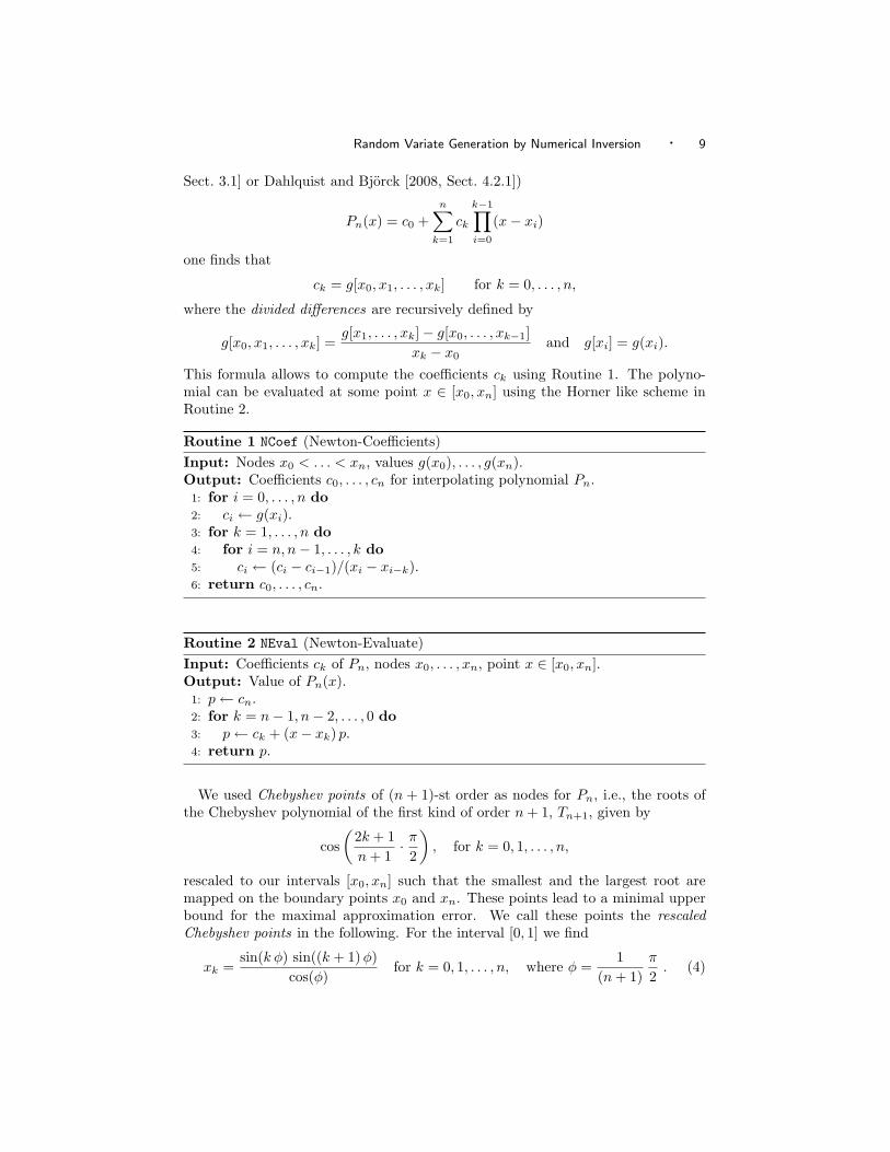
Sect. 3.1] or Dahlquist and Bjorck [2008, Sect. 4.2.1])
Pn(x) = c0 +n∑k=1
ck
k−1∏i=0
(x− xi)
one finds that
ck = g[x0, x1, . . . , xk] for k = 0, . . . , n,
where the divided differences are recursively defined by
g[x0, x1, . . . , xk] =g[x1, . . . , xk]− g[x0, . . . , xk−1]
xk − x0and g[xi] = g(xi).
This formula allows to compute the coefficients ck using Routine 1. The polyno-mial can be evaluated at some point x ∈ [x0, xn] using the Horner like scheme inRoutine 2.
Routine 1 NCoef (Newton-Coefficients)Input: Nodes x0 < . . . < xn, values g(x0), . . . , g(xn).Output: Coefficients c0, . . . , cn for interpolating polynomial Pn.
1: for i = 0, . . . , n do2: ci ← g(xi).3: for k = 1, . . . , n do4: for i = n, n− 1, . . . , k do5: ci ← (ci − ci−1)/(xi − xi−k).6: return c0, . . . , cn.
Routine 2 NEval (Newton-Evaluate)Input: Coefficients ck of Pn, nodes x0, . . . , xn, point x ∈ [x0, xn].Output: Value of Pn(x).
1: p← cn.2: for k = n− 1, n− 2, . . . , 0 do3: p← ck + (x− xk) p.4: return p.
We used Chebyshev points of (n + 1)-st order as nodes for Pn, i.e., the roots ofthe Chebyshev polynomial of the first kind of order n+ 1, Tn+1, given by
cos(
2k + 1n+ 1
· π2
), for k = 0, 1, . . . , n,
rescaled to our intervals [x0, xn] such that the smallest and the largest root aremapped on the boundary points x0 and xn. These points lead to a minimal upperbound for the maximal approximation error. We call these points the rescaledChebyshev points in the following. For the interval [0, 1] we find
xk =sin(k φ) sin((k + 1)φ)
cos(φ)for k = 0, 1, . . . , n, where φ =
1(n+ 1)
π
2. (4)

10 · G. Derflinger, W. Hormann, and J. Leydold
3.2 Inverse Interpolation
For an interval [F (ak−1), F (ak)] we apply Newton’s interpolation formula, to con-struct an approximating polynomial F−1
a for the inverse CDF F−1. For the nodeswe use ui = F (xi) where xi are the rescaled Chebyshev points on the interval[ak−1, ak]. The values of F−1 at the nodes are F−1(ui) = xi. This approach avoidsthe evaluation of the inverse CDF. Moreover, it leads to close to minimal approxi-mation errors where F is nearly linear within an interval [ak−1, ak] (which is oftenthe case for the center of the distribution). It may lead to larger than optimal errorsin other parts, in particular in the tails, but it is still better than using equidistantui. A disadvantage is that we have to store the values of ui in a table (see alsoRemark 3 below). We finally decided to use this simple approach as it leads to astable setup.
The estimation of the interpolation error is a crucial part of an automatic algo-rithm. As direct consequence of (3) we find for the x-error
εx(u) = |F−1(u)− F−1a (u)| = |(F
−1)(n+1)(ζ)|(n+ 1)!
n∏i=0
|u− ui| (5)
where (F−1)(n+1)(ζ) =(ddv
)n+1F−1(v)
∣∣v=ζ
denotes the n+ 1st derivate of F−1 atsome point ζ ∈ [F (ak−1), F (ak)]. Hence we obtain an upper bound for the u-errorof the approximation.
Lemma 1. Let F−1a be a polynomial of order n, approximating F−1 over [F (ak−1),
F (ak)] for some interval [ak−1, ak], as described above. Assume that F−1 is n+ 1-times continuously differentiable. If F−1 and F−1
a have the same image, then
εu(u) ≤ maxx∈[ak−1,ak]
v∈[F (ak−1),F (ak)]
f(x)|(F−1)(n+1)(v)|
(n+ 1)!
n∏i=0
|u− ui| . (6)
Notice that the last condition is satisfied when F−1a is monotone, since F−1 and
F−1a coincide on F (ak−1) and F (ak).
Proof. Let u ∈ [F (ak−1), F (ak)] and ua = F (F−1a (u)). Then εu(u) = |u − ua|
and εx(u) = |F−1(u) − F−1(ua)|. Hence by the mean value theorem there existsa ζ ∈ (u, ua) such that εx(u)/εu(u) = (F−1)′(ζ) = 1/F ′(ξ) = 1/f(ξ) where ξ =F−1(ζ). As F−1 and F−1
a have the same image, we find ξ ∈ [ak−1, ak] and thusεu(u) ≤ maxx∈[ak−1,ak] f(x) εx(u). Hence the result follows from (5).
It is possible to use this bound to derive rigorous error bounds on the approximationerror as the derivatives of F−1 can be calculated using only derivatives of f(x) bymeans of Faa di Bruno’s formula (see Sect. 3.7 below for an example). However,computing and implementing higher order derivatives is quite tedious for all andvirtually impossible for many densities. Thus it is not a convenient ingredient of ablack-box algorithm.
We therefore also consider, how to estimate the u-error without using the abovebound. Instead it is useful to consider the approximation
εu(u) ≈ f(F−1(u)) εx(u) ≈ f(F−1(u))|(F−1)(n+1)(u)|
(n+ 1)!
n∏i=0
|u− ui| .

Random Variate Generation by Numerical Inversion · 11
For many distributions we made the following observation: For (very) short inter-vals, compared to
∏ni=0(u − ui), the term f(F−1(u)) (F−1)(n+1)(u) has only little
influence on εu(u). (If this is not the case, then the interpolation error is large andwe have to use a shorter interval anyway.) Thus the maximal u-error in a shortinterval is attained very close to the extrema of
∏ni=0 |u− ui| that we denote by ti,
i = 1, . . . , n. We can therefore use
u-error ≈ maxi=1,...,n
|ti − Fi(F−1a (ti))| (7)
as a simple estimate for the u-error of the interpolation. Here Fi denotes theapproximate CDF computed using numerical integration of the PDF.
For the polynomial p(u) =∏ni=0(u− ui) we find
p′(u) =n∑k=0
n∏i=0i6=k
(u− ui) = p(u)n∑k=0
1u− uk
.
Since the points u0 < . . . < un are distinct, p′(u) cannot be zero at uk, k = 0, . . . n.Thus we only need to find the roots of
∑nk=0
1u−uk
(approximately). We found outthat this can be done efficiently using only two iterations of Newton’s root findingmethod, where starting with ti = (ui−1 + ui)/2 we use the recursion
ti,new = ti +∑nk=0(1/(ti − uk))∑nk=0(1/(ti − uk)2)
.
The entire algorithm for computing the test points ti is compiled in Routine 3.
Routine 3 NTest (Newton-Testpoints)Input: Nodes u0 < . . . < un.Output: Test points t1 < . . . < tn.
1: for i = 1, . . . , n do2: ti ← (ui−1 + ui)/2.3: for j = 1, 2 do . 2 Newton steps
4: s← 0, sq ← 0.5: for k = 0, . . . , n do6: s← s+ 1/(ti − uk), sq ← sq + 1/(ti − uk)2.7: ti ← ti + s/sq.8: return t1, . . . , tn.
Heuristic (7) works for quite a large class of simulation problems. However,although based on some mathematical arguments there is no guarantee that itworks reliably for every distribution.
Notice that the computation of the first derivative of εu(u) only requires oneevaluation of the density and one of the derivative of the interpolating polynomial.The derivative can be calculated by inserting only two additional statements intoRoutine 2: p′ ← 0 (initialize p′) before the loop is started and p′ ← p+ (t− xk) p′
(apply the product rule) as first statement within the loop. The resulting modifiedRoutine 2 returns the value p of the interpolating polynomial at x and its derivativep′, as well. As the error is known to be zero at ui we can use the very stable bisection

12 · G. Derflinger, W. Hormann, and J. Leydold
method with starting interval [ui−1, ui] to find the root of the derivative of εu(u)and thus the local maximum in that region. This method works reliably as longas this maximum is unique in each of the subintervals [ui−1, ui]. Of course thenumerical search for the n local extrema of the u-error requires a lot of evaluationsof the density and thus slows down the setup considerably. It is interesting thatin most cases this method leads to the same decomposition of the domain intointervals [ak−1, ak] as evaluating the u-error only at the testpoints.
Note that it is not easy to decide between the two variants: numerical search foreach local maximum of the u-error, or evaluation of the u-error only at the testpoints. It is a tradeoff between setup time and (more) reliable error control. Asour empirical results for the simple error control were always satisfying we decidedto use it as default method for our algorithm.
Monotonicity of the approximated inverse CDF, F−1a , might also be an issue for
some applications. There exists a lot of literature on shape-preserving (mostly cu-bic) spline interpolation. However, methods for constructing monotone polynomialsthat interpolate monotone points are rather complicated (e.g., Costantini [1986]).Thus we have decided to use a rather simple technique and only check the mono-tonicity at the points F−1
a (ti) that we already use in (7) for estimating the u-error.If monotonicity is of major importance for an application, it is possible to checkfor monotonicity by evaluating the first derivative of the approximating polynomial(which is easy as mentioned above) at many points, or by searching numerically fornegative values of that derivative.
To increase the numeric stability of the interpolation of the inverse CDF we usea transformed version Fk of the CDF on each interval [ak−1, ak]. Therefore wedefine Fk(x) = F (x + ak−1) − F (ak−1) =
∫ ak−1+x
ak−1f(t) dt for x ∈ [0, ak − ak−1].
Then the problem of inverting F (x) on [ak−1, ak] is equivalent to inverting Fk(x)on [0, ak − ak−1]: for a u ∈ [F (ak−1), F (ak)] we get F−1(u) by
F−1(u) = ak−1 + F−1k (u− F (ak−1)) .
This transformation has two advantages. The computation of Fk(x) by integrating∫ ak−1+x
ak−1f(t) dt is numerically more stable because the subtraction F (x + ak−1) −
F (ak−1), that might cause loss of accuracy, is no longer necessary. This improvesin particular the numeric precision in the right tail of the distribution. Moreover,the first node of our interpolation problem is always (0, 0) which saves memory andcomputations.
Remark 2. We use linear interpolation as a fallback when Newton’s interpolationformula fails due to numerical errors.
Remark 3. An alternative approach is to use the optimal interpolation points,i.e., the Chebyshev points rescaled for the interval [F (ak−1), F (ak)]. This is conve-nient as, up to a linear transformation, they are the same for all intervals and weneed not store them in a table. Moreover, this also holds for the test points ti forthe error estimate (7) and, therefore, we would not need Routine NTest. However,the main drawback of this alternative is that we have to invert the CDF to calcu-late xi = F−1(ui) which may lead to numerical problems due to rounding errorsespecially in the tails.
Random Variate Generation by Numerical Inversion · 13
Remark 4. We also made experiments with other interpolations. However, wehave decided against these alternatives. Hermite interpolation (see [Hormann andLeydold 2003]) has slightly larger u-errors for a given order of polynomial andrequires (higher order) derivatives of the density. Moreover, it was numerically lessstable in regions with flat densities, especially in the tails of the distribution. Onthe other hand, continued fractions have the advantage that we can extrapolatetowards poles but we were not able to estimate interpolation errors during thesetup.
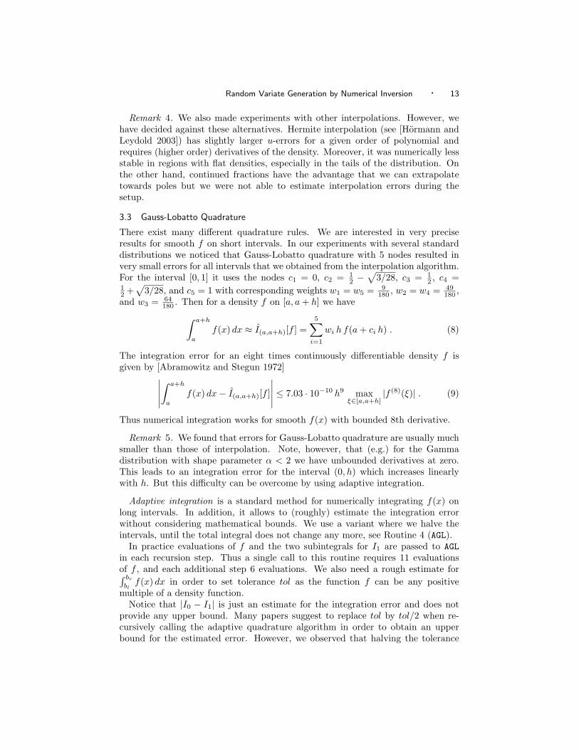
3.3 Gauss-Lobatto Quadrature
There exist many different quadrature rules. We are interested in very preciseresults for smooth f on short intervals. In our experiments with several standarddistributions we noticed that Gauss-Lobatto quadrature with 5 nodes resulted invery small errors for all intervals that we obtained from the interpolation algorithm.For the interval [0, 1] it uses the nodes c1 = 0, c2 = 1
2 −√
3/28, c3 = 12 , c4 =
12 +√
3/28, and c5 = 1 with corresponding weights w1 = w5 = 9180 , w2 = w4 = 49
180 ,and w3 = 64
180 . Then for a density f on [a, a+ h] we have∫ a+h
a
f(x) dx ≈ I(a,a+h)[f ] =5∑i=1
wi h f(a+ ci h) . (8)
The integration error for an eight times continuously differentiable density f isgiven by [Abramowitz and Stegun 1972]∣∣∣∣∣
∫ a+h
a
f(x) dx− I(a,a+h)[f ]
∣∣∣∣∣ ≤ 7.03 · 10−10 h9 maxξ∈[a,a+h]
|f (8)(ξ)| . (9)
Thus numerical integration works for smooth f(x) with bounded 8th derivative.
Remark 5. We found that errors for Gauss-Lobatto quadrature are usually muchsmaller than those of interpolation. Note, however, that (e.g.) for the Gammadistribution with shape parameter α < 2 we have unbounded derivatives at zero.This leads to an integration error for the interval (0, h) which increases linearlywith h. But this difficulty can be overcome by using adaptive integration.
Adaptive integration is a standard method for numerically integrating f(x) onlong intervals. In addition, it allows to (roughly) estimate the integration errorwithout considering mathematical bounds. We use a variant where we halve theintervals, until the total integral does not change any more, see Routine 4 (AGL).
In practice evaluations of f and the two subintegrals for I1 are passed to AGLin each recursion step. Thus a single call to this routine requires 11 evaluationsof f , and each additional step 6 evaluations. We also need a rough estimate for∫ br
blf(x) dx in order to set tolerance tol as the function f can be any positive
multiple of a density function.Notice that |I0 − I1| is just an estimate for the integration error and does not
provide any upper bound. Many papers suggest to replace tol by tol/2 when re-cursively calling the adaptive quadrature algorithm in order to obtain an upperbound for the estimated error. However, we observed that halving the tolerance

14 · G. Derflinger, W. Hormann, and J. Leydold
Routine 4 AGL (Adaptive-Gauss-Lobatto)Input: Density f(x), domain [a, a+ h], tolerance tol.Output:
∫ a+ha
f(x) dx with estimated maximal error less than tol.1: I0 ← I(a,a+h)[f ].2: I1 ← I(a,a+h/2)[f ] + I(a+h/2,a+h)[f ].3: if |I0 − I1| < tol then4: return I1.5: else6: return (AGL(f , (a, a+ h/2), tol) + AGL(f , (a+ h/2, a+ h), tol)).
leads to severe problems for distributions with heavy tails (e.g., the Cauchy distri-bution) where it never reaches the precision goal. Thus we followed the version ofadaptive integration described by Gander and Gautschi [2000]. They argue1 thathalving the tolerance for every subdivision leads to lots of unnecessary functionevaluations without providing an upper bound for the (true) integration error, thatis not available with that type of error bound anyway. In all our experiments, theerrors when using Routine 4 were smaller than required. We have even observedin our experiments that for nearly all cases the intervals for Newton’s interpolationformula are adequately short for simple (non-adaptive) Gauss-Lobatto quadrature(8) to obtain sufficient accuracy. However, for distributions with high tails (e.g.,Cauchy) or unbounded derivatives (e.g., Gamma with shape parameter α close toone) we needed adaptive integration. The following procedure was quite efficientthen:
0. Roughly compute I0 = I(bl,br)[f ] to get maximal tolerated error tol.
1. Compute I(bl,br)[f ] with required accuracy by adaptive Gauss-Lobatto quadra-ture using Routine AGL and store subinterval boundaries and CDF values. Weused tol = 0.05 I0 εu.
2. When integrals I(xj−1,xj)[f ] have to be computed we use the intervals and theCDF values from Step 1 above together with simple Gauss-Lobatto quadrature.
Remark 6. There exist many other quadrature rules as well. Some of thesemay be a suitable replacement. However, the arguments for our procedure are asfollowing:
—Adaptive integration provides flexibility. It works for (sufficiently smooth) den-sities without further interventions.
—Using the same quadrature rule for each recursion of adaptive integration as wellas for the simple quadrature rule allows to store and reuse intervals and CDFvalues. Thus we have sufficient accuracy with simple quadrature on arbitrarysubintervals.
—The boundary points of the intervals should be used as nodes of adaptive quadra-ture. Thus they can be reused for further recursion steps.
1Private communication from Walter Gander.
Random Variate Generation by Numerical Inversion · 15
—The number of nodes for the (simple) quadrature rule should in most cases pro-vide sufficient accuracy for the integrals between the construction points of theinterpolating polynomials; but not more to avoid futile density evaluations.
For these reasons we have rejected Gauss-Legendre quadrature with 4 nodes. Ithas an integration error similar to Gauss-Lobatto quadrature with 5 nodes but asthe latter uses the interval endpoints as nodes it is especially suited for recursivesubdivisions of the intervals. Then it requires only 6 additional evaluations of fin opposition to Gauss-Legendre where 8 evaluations are necessary. Moreover forGauss-Lobatto quadrature three of the 5 nodes and all weights are rational numbersand can be stored without rounding errors.
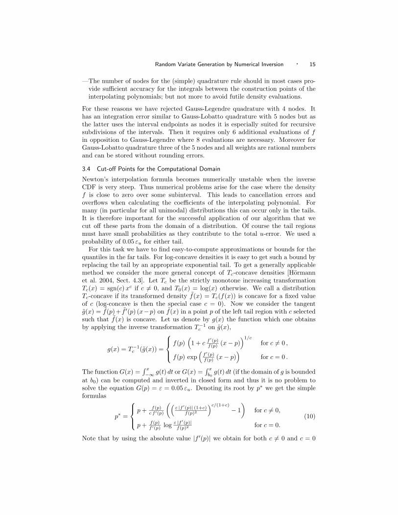
3.4 Cut-off Points for the Computational Domain
Newton’s interpolation formula becomes numerically unstable when the inverseCDF is very steep. Thus numerical problems arise for the case where the densityf is close to zero over some subinterval. This leads to cancellation errors andoverflows when calculating the coefficients of the interpolating polynomial. Formany (in particular for all unimodal) distributions this can occur only in the tails.It is therefore important for the successful application of our algorithm that wecut off these parts from the domain of a distribution. Of course the tail regionsmust have small probabilities as they contribute to the total u-error. We used aprobability of 0.05 εu for either tail.
For this task we have to find easy-to-compute approximations or bounds for thequantiles in the far tails. For log-concave densities it is easy to get such a bound byreplacing the tail by an appropriate exponential tail. To get a generally applicablemethod we consider the more general concept of Tc-concave densities [Hormannet al. 2004, Sect. 4.3]. Let Tc be the strictly monotone increasing transformationTc(x) = sgn(c)xc if c 6= 0, and T0(x) = log(x) otherwise. We call a distributionTc-concave if its transformed density f(x) = Tc(f(x)) is concave for a fixed valueof c (log-concave is then the special case c = 0). Now we consider the tangentg(x) = f(p)+ f ′(p) (x−p) on f(x) in a point p of the left tail region with c selectedsuch that f(x) is concave. Let us denote by g(x) the function which one obtainsby applying the inverse transformation T−1
c on g(x),
g(x) = T−1c (g(x)) =
f(p)
(1 + c f
′(p)f(p) (x− p)
)1/c
for c 6= 0 ,
f(p) exp(f ′(p)f(p) (x− p)
)for c = 0 .
The function G(x) =∫ x−∞ g(t) dt or G(x) =
∫ xb0g(t) dt (if the domain of g is bounded
at b0) can be computed and inverted in closed form and thus it is no problem tosolve the equation G(p) = ε = 0.05 εu. Denoting its root by p∗ we get the simpleformulas
p∗ =
p+ f(p)
c f ′(p)
((ε |f ′(p)| (1+c)
f(p)2
)c/(1+c)− 1)
for c 6= 0,
p+ f(p)f ′(p) log ε |f ′(p)|
f(p)2 for c = 0.(10)
Note that by using the absolute value |f ′(p)| we obtain for both c 6= 0 and c = 0

16 · G. Derflinger, W. Hormann, and J. Leydold
a single formula applicable for both, the right and the left tail. The result p∗ canbe used as new value for p thus defining a simple recursion that converges very fastclose to exact results.
We have assumed above that c was selected such that f is Tc-concave (i.e. f(x)is concave). Then the function g(x) is an upper bound for f(x). This clearlyimplies that p∗ is always a lower bound for the quantile in the left tail and anupper bound for the quantile in the right tail. Thus the resulting value p∗ of thedescribed method is guaranteed to cut off less than the desired probability 0.05 εuif the required constant c is known. This is the case, e.g., for the Normal, beta andgamma distributions that are all log-concave (c = 0). For the t-distribution withν degrees of freedom it is easy to show that it is Tc-concave for c = −1/(1 + ν).We tested the cut-off procedure for all these distributions and obtained very closebounds for the required quantiles. To be precise the cut-off procedure above doesnot require that the density is Tc-concave everywhere, it is enough that it is Tc-concave in the tail.
Of course it is possible that the value of c that leads to a Tc-concave tail isnot known. Fortunately, this situation can be solved by means of the conceptof local concavity of a density f at a point x [Hormann et al. 2004, Sect. 4.3].The local concavity is the maximal value for c such that the transformed densityf(x) = Tc(f(x)) is concave near x. For a twice differentiable density f it is givenby
lcf (x) = 1− f ′′(x) f(x)f ′(x)2
and can be calculated sufficiently accurately by using
lcf (x) = limδ→0
(f(x+ δ)
f(x+ δ)− f(x)+
f(x− δ)f(x− δ)− f(x)
)− 1 .
Taylor series expansion reveals that the approximation error is O(δ2) if f is fourtimes continuously differentiable.
Notice that in the left tail f(x) is concave for x ≤ p whenever lcf (x) ≥ c for allx ≤ p. If we assume that lcf (x) is approximately constant in the far tails we canuse the recursion (10) with c = lcf (x). Of course the resulting cut-off value is nolonger guaranteed to be the bound of the required quantile as we do not have anassumption on the tail behavior of f . Still that approach works correctly and isstable for the distributions we tried.
Remark 7. There is no need for a cut-off point when the domain is boundedfrom the left by bl, and f(bl) or f ′(bl) is greater than zero. Analogously for a rightboundary br.
3.5 Construct Subintervals for Piecewise Interpolation
We have to subdivide the domain of the distribution into intervals [ai−1, ai], i =1, . . . k, with bl = a0 < a1 < . . . < ak = br. We need sufficiently short intervals toreach our accuracy goal. On the other hand many intervals result in large tables.We use a simple technique to solve this problem: We construct the intervals startingfrom the left boundary point of the domain and proceed to its right boundary. Westart with some initial interval length, compute the interpolating polynomial and

Random Variate Generation by Numerical Inversion · 17
estimate the error using (7). If the error is larger than εu we have to shorten theinterval and try again. Otherwise we fix that interval and store its interpolationcoefficients and proceed to the next interval. If the error for the last interval wasmuch smaller than required we try a slightly longer one now.
Remark 8. An alternative approach is interval bisection: Start with a partitionof the (computational) domain [bl, br]. Whenever the u-error is too large in ainterval it is split into two subintervals. This procedure is used in [Hormann andLeydold 2003] (where the CDF is directly available) but results in a larger numberof intervals and thus larger tables. For the setting of this paper, where we start fromthe PDF and combine numeric integration with interpolation, interval bisection isless suited.
3.6 Adjust Error Bounds
We have several sources of numerical error: Cutting off tails, integration errors andinterpolation errors. As we want to control the maximal error we have to adjust thetolerated u-error in each of these steps. Let εu denote the requested u-resolution.Then we use εu = 0.9 εu for the maximal tolerated error for the interpolation erroras computed in (7). For the probabilities of the truncated tails we use 0.05 εu andfor the integration error we allow at most 0.05 I0 εu. By this strategy the totalu-error was always below εu for all our test distributions (when εu ≥ 10−12).
We can conclude from bound (6) that the number of intervals will be moderatefor interpolation of order n if the density has a bounded n-th derivative (or canbe decomposed into intervals with bounded n-th derivative). The number of nec-essary intervals may get very large if that assumption is not fulfilled but still theinterpolation error converges to zero when the interval lengths are tending to zero.
For Gauss-Lobatto integration bound (9) indicates that a bounded eighth deriva-tive is required to obtain fast convergence. Otherwise the number of intervals of ouralgorithm remains unchanged but a large number of subdivisions and evaluations ofthe density may be required in the adaptive integration algorithm Routine 4. Theintegration error tends to zero if the number of subdivisions is increased furtherand further for any continuous bounded density f .
3.7 Rigorous Bounds
We have described both rigorous mathematical bounds and convenient approxima-tions to assess the maximal u-error of an inversion algorithm. As these approxi-mations lead to precise error estimates in our experiments and are much easier touse, we mainly considered the details of that approach. Still this should not givethe wrong impression that it is not possible to calculate and use the exact mathe-matical bounds given above. As a matter of fact we can calculate the exact errorbounds for any density f that is sufficiently smooth (i.e., it has bounded eighthderivative) if we can evaluate the eighth derivative of f . (This is no problem inpractice if f can be written in closed form.) We demonstrate here the use of thosebounds to develop the inversion algorithm for a prominent example, the standardnormal distribution. It works analogously for other distributions provided that therespective CDF and density are “sufficiently nice”.
We first have to fix the requested u-resolution εu and the order n of the in-
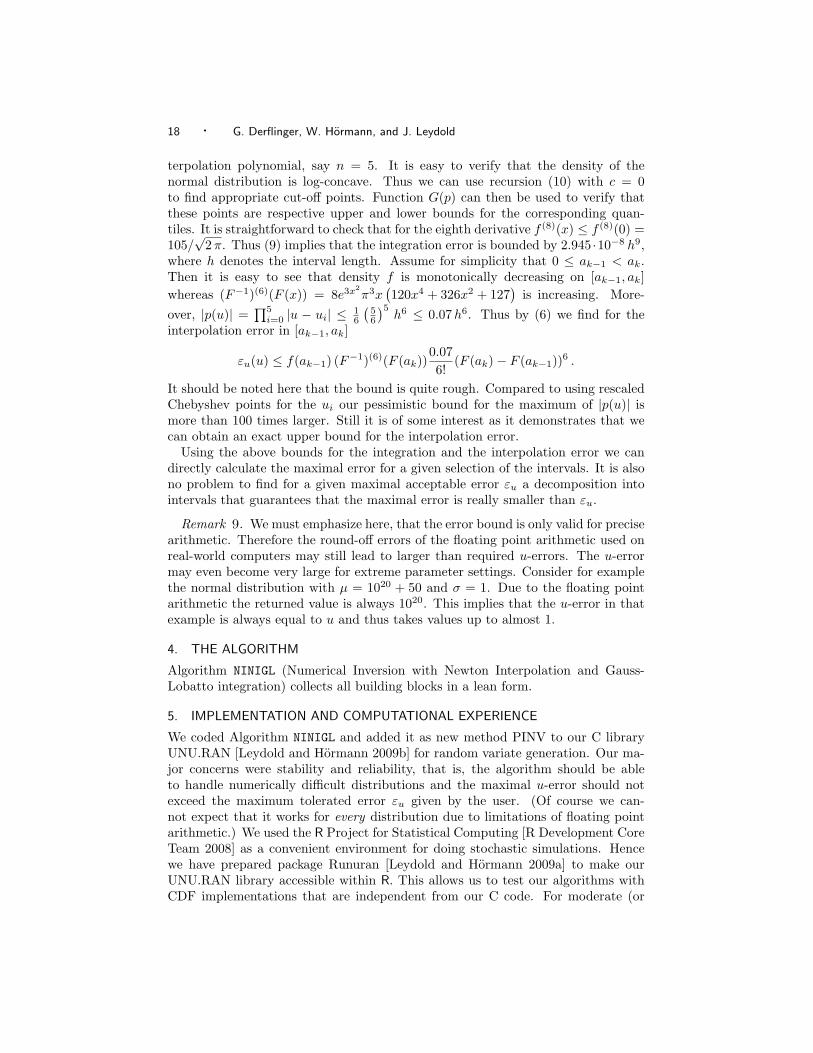
18 · G. Derflinger, W. Hormann, and J. Leydold
terpolation polynomial, say n = 5. It is easy to verify that the density of thenormal distribution is log-concave. Thus we can use recursion (10) with c = 0to find appropriate cut-off points. Function G(p) can then be used to verify thatthese points are respective upper and lower bounds for the corresponding quan-tiles. It is straightforward to check that for the eighth derivative f (8)(x) ≤ f (8)(0) =105/
√2π. Thus (9) implies that the integration error is bounded by 2.945 ·10−8 h9,
where h denotes the interval length. Assume for simplicity that 0 ≤ ak−1 < ak.Then it is easy to see that density f is monotonically decreasing on [ak−1, ak]whereas (F−1)(6)(F (x)) = 8e3x
2π3x
(120x4 + 326x2 + 127
)is increasing. More-
over, |p(u)| =∏5i=0 |u − ui| ≤
16
(56
)5h6 ≤ 0.07h6. Thus by (6) we find for the
interpolation error in [ak−1, ak]
εu(u) ≤ f(ak−1) (F−1)(6)(F (ak))0.076!
(F (ak)− F (ak−1))6 .
It should be noted here that the bound is quite rough. Compared to using rescaledChebyshev points for the ui our pessimistic bound for the maximum of |p(u)| ismore than 100 times larger. Still it is of some interest as it demonstrates that wecan obtain an exact upper bound for the interpolation error.
Using the above bounds for the integration and the interpolation error we candirectly calculate the maximal error for a given selection of the intervals. It is alsono problem to find for a given maximal acceptable error εu a decomposition intointervals that guarantees that the maximal error is really smaller than εu.
Remark 9. We must emphasize here, that the error bound is only valid for precisearithmetic. Therefore the round-off errors of the floating point arithmetic used onreal-world computers may still lead to larger than required u-errors. The u-errormay even become very large for extreme parameter settings. Consider for examplethe normal distribution with µ = 1020 + 50 and σ = 1. Due to the floating pointarithmetic the returned value is always 1020. This implies that the u-error in thatexample is always equal to u and thus takes values up to almost 1.
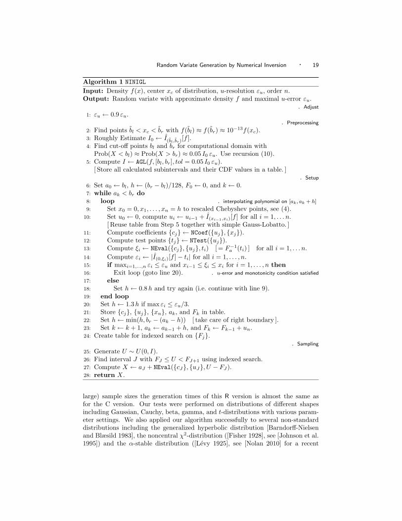
4. THE ALGORITHM
Algorithm NINIGL (Numerical Inversion with Newton Interpolation and Gauss-Lobatto integration) collects all building blocks in a lean form.
5. IMPLEMENTATION AND COMPUTATIONAL EXPERIENCE
We coded Algorithm NINIGL and added it as new method PINV to our C libraryUNU.RAN [Leydold and Hormann 2009b] for random variate generation. Our ma-jor concerns were stability and reliability, that is, the algorithm should be ableto handle numerically difficult distributions and the maximal u-error should notexceed the maximum tolerated error εu given by the user. (Of course we can-not expect that it works for every distribution due to limitations of floating pointarithmetic.) We used the R Project for Statistical Computing [R Development CoreTeam 2008] as a convenient environment for doing stochastic simulations. Hencewe have prepared package Runuran [Leydold and Hormann 2009a] to make ourUNU.RAN library accessible within R. This allows us to test our algorithms withCDF implementations that are independent from our C code. For moderate (or
Random Variate Generation by Numerical Inversion · 19
Algorithm 1 NINIGL
Input: Density f(x), center xc of distribution, u-resolution εu, order n.Output: Random variate with approximate density f and maximal u-error εu.
. Adjust
1: εu ← 0.9 εu.. Preprocessing
2: Find points bl < xc < br with f(bl) ≈ f(br) ≈ 10−13f(xc).3: Roughly Estimate I0 ← I(bl,br)[f ].4: Find cut-off points bl and br for computational domain with
Prob(X < bl) ≈ Prob(X > br) ≈ 0.05 I0 εu. Use recursion (10).5: Compute I ← AGL(f, [bl, br], tol = 0.05 I0 εu).
[ Store all calculated subintervals and their CDF values in a table. ]. Setup
6: Set a0 ← bl, h← (br − bl)/128, F0 ← 0, and k ← 0.7: while ak < br do8: loop . interpolating polynomial on [ak, ak + h]
9: Set x0 = 0, x1, . . . , xn = h to rescaled Chebyshev points, see (4).10: Set u0 ← 0, compute ui ← ui−1 + I(xi−1,xi)[f ] for all i = 1, . . . n.
[ Reuse table from Step 5 together with simple Gauss-Lobatto. ]11: Compute coefficients {cj} ← NCoef({uj}, {xj}).12: Compute test points {tj} ← NTest({uj}).13: Compute ξi ← NEval({cj}, {uj}, ti) [ = F−1
a (ti) ] for all i = 1, . . . n.14: Compute εi ← |I(0,ξi)[f ]− ti| for all i = 1, . . . , n.15: if maxi=1,...,n εi ≤ εu and xi−1 ≤ ξi ≤ xi for i = 1, . . . , n then16: Exit loop (goto line 20). . u-error and monotonicity condition satisfied
17: else18: Set h← 0.8h and try again (i.e. continue with line 9).19: end loop20: Set h← 1.3h if max εi ≤ εu/3.21: Store {cj}, {uj}, {xn}, ak, and Fk in table.22: Set h← min(h, br − (ak − h)) [ take care of right boundary ].23: Set k ← k + 1, ak ← ak−1 + h, and Fk ← Fk−1 + un.24: Create table for indexed search on {Fj}.
. Sampling
25: Generate U ∼ U(0, I).26: Find interval J with FJ ≤ U < FJ+1 using indexed search.27: Compute X ← aJ + NEval({cJ}, {uJ}, U − FJ).28: return X.
large) sample sizes the generation times of this R version is almost the same asfor the C version. Our tests were performed on distributions of different shapesincluding Gaussian, Cauchy, beta, gamma, and t-distributions with various param-eter settings. We also applied our algorithm successfully to several non-standarddistributions including the generalized hyperbolic distribution [Barndorff-Nielsenand Blæsild 1983], the noncentral χ2-distribution ([Fisher 1928], see [Johnson et al.1995]) and the α-stable distribution ([Levy 1925], see [Nolan 2010] for a recent

20 · G. Derflinger, W. Hormann, and J. Leydold
Table I. Required number of intervals for different u-resolutions εu using polynomials of order 1,
3 and 5, respectively.εu 10−8 10−10 10−8 10−10 10−12 10−8 10−10 10−12
distribution Order n = 1 Order n = 3 Order n = 5
Normal 12620 118294 173 517 1603 63 123 252
Cauchy 19512 193558 288 826 2504 112 203 393Exponential 10914 108882 128 382 1192 44 87 176
Gamma(5) 11890 121602 177 526 1647 62 124 255
Beta(5,5) 11272 99702 155 477 1491 58 114 236Beta(5,500) 11874 11130 178 527 1648 62 124 256
survey).In extensive tests we observed that for all these distributions our algorithm re-
sults in approximations that have u-errors smaller than the one required by the user.u-resolutions of 10−12 were reached without problems for all the mentioned distri-butions. The set-up time is moderate and strongly depends on the time needed toevaluate the density f . The marginal execution times are very fast and practicallythe same for all tested distributions. The marginal execution times we observedwere all faster than generating an exponential random variate by inversion.
The interested reader can find more information on the distributions we tested,on the results of our stability and accuracy tests and on the speed of the setup andof the sampling algorithm in the Online Supplement of this article.
5.1 The Required Number of Intervals
The required number of intervals is an important characteristic of the algorithmas it influences both the setup time and the size of the required table. Using theerror-bound for interpolation which is O(hn+1) for interval length h and order n itis obvious that the required number of intervals is O(1/εn+1
u ). This implies that forlinear interpolation an error-reduction by a factor of 1/100 requires about ten timesthe number of intervals. Therefore, linear interpolation is not useful if small errorvalues are required as the table sizes explode. For order n = 3 an error-reductionby a factor of 1/100 requires
√10 = 3.16 times the number of intervals, for n = 5
this factor is reduced to 3√
10 = 2.16. In Table I we report the required numberof intervals for some standard distributions and practically important values ofεu. These results clearly illustrate the asymptotic considerations for the requirednumber of intervals. They also indicate that order n = 5 is enough to reach closeto machine precision with a moderate number of intervals. Of course larger valuesof n are not desirable as they would lead to slower marginal execution times. Notethat the speed differences between n = 1, n = 3 and n = 5 were close to negligiblein our timing experiments.
The differences between distributions are not too large. The worst case of ourexamples is the Cauchy distribution whose heavy tails imply a large computation-ally relevant domain and thus many intervals. Otherwise the differences are small,monotone densities (like the exponential density) and densities without tail (likethe Beta(5,5) density) require slightly less intervals than bell-shaped densities withtwo tails.

Random Variate Generation by Numerical Inversion · 21
6. COMPARISON WITH UNIVERSAL ALGORITHMS OF THE LITERATURE
We have already pointed out that the automatic inversion algorithms described byAhrens and Kohrt [1981] and Ulrich and Watson [1987] are based on similar ideasas our algorithm. They use a decomposition into many intervals and polynomialapproximations of the inverse CDF within those intervals. The main difference toour algorithm is that all of their algorithms use a decomposition fixed at the be-ginning, whereas we select the decomposition such that the maximal error is belowa user-selected threshold. Moreover, there is no further control of the resultingapproximation error.
The algorithm by Ahrens and Kohrt [1981] is based on Lagrange interpolationon nine points in each of the intervals. The interpolating polynomials are thenapproximated by a truncated expansion into Chebyshev polynomials, the high-est order polynomials are discarded as long as the sum of the absolute values ofthe neglected coefficients is below the required accuracy, and the remaining partsare reconverted into common polynomials. Thus the order of the approximatingpolynomials vary between different intervals to reach what they claim to be exactinversion for single precision. The cut-off points for the computational domain arefound by a simple strategy. The algorithm requires the evaluation of the inverseCDF in the setup which is performed with a method that is related to Newton’sroot finding. The paper states that it “require[s] a double precision integrationroutine” for computing the CDF and that “iterated Simpson integration provedadequate”.
Ulrich and Watson [1987] describe several numeric inversion methods. Besidesusing a packaged ODE solver they also developed fourth and fifth order Runge-Kutta type approximations to the inverse CDF based on the integration of the ODEx′(u) = 1/f(x(u)). All their algorithms are based on the same fixed subdivision ofdomain (0, 1) as the method of Ahrens and Kohrt [1981]. A last approach presentedthere is the usage of B-splines which are available in many scientific software pack-ages. Again the same fixed subdivision is used to compute a first approximation.This is then used to find near optimal knot placement for the final B-spline approxi-mation. One of the appealing features of the B-spline approximation scheme is thatthe kth order B-spline will have a continuous (k − 2)nd derivative and hence willprovide a very smooth approximation to the inverse CDF. An obvious drawback is,that one cannot make local adaptive improvements of the approximation accuracyas in [Hormann and Leydold 2003] or our new algorithm.
Ulrich and Watson [1987] report the x-errors of these algorithms. The maxi-mal reported x-errors are all above 10−5 which cannot be called close to machineprecision. They also report the maximal x-error of the algorithm of Ahrens andKohrt [1981] which is always larger than 10−2 and mention that there is a problemwith the precision in the tails. Both papers do not give a detailed description ofthe full algorithms and we were not able to get the original implementations. It isthus impossible for us to assess the speed and the exact size of the error of thosealgorithms.
Still we want to underline, that we consider the capability of the user to selectthe acceptable maximal u-error, which may be close to machine precision, as themain achievement of our new algorithm.
22 · G. Derflinger, W. Hormann, and J. Leydold
As linear interpolation, despite its unbeatable simplicity, is not capable to reachhigh precision with moderate tables (compare the required number of intervals inTable I), we compare our new algorithm only to our first numeric inversion al-gorithm HINV based on Hermite interpolation (see [Hormann and Leydold 2003];it is also implemented in our UNU.RAN library). A main difference to the newalgorithm is that HINV requires the CDF and PDF for order n = 3 polynomialsand also the derivative of the PDF for order n = 5; orders higher than 5 are notpossible. A main reason for developing the new algorithm was that obtaining aprecise implementation of the CDF is not easy for most important distributions.Combining it just with some numerical integrator when only the PDF is availablewas discouraging slow with, e.g., the generalized hyperbolic and the noncentral χ2-distribution. Using the CDF allows a simpler cut-off procedure and avoids possibleintegration errors, but interestingly it does not improve the stability of the algo-rithm. Especially in the right tail the numerical instabilities of HINV are largerthan those of our new algorithm. This is underlined by the fact that we observedseveral cases with u-errors larger than εu (about five percent of all cases we com-puted) when we tested the u-error of HINV in the tails of the distribution. For someparameter values of the t-distribution and εu = 10−13 HINV is not able to reachthe required accuracy and decomposes the domain into a huge number of intervalswhich never happened for our new algorithm. The numeric instabilities come fromthe fact that in the far right tail the CDF is only calculated with a precision of10−16 and the probabilities of the intervals are small. Numeric integration in ournew algorithm reduces that problem as we are calculating the CDF starting onlywith the left border of the current interval.
The marginal generation times of HINV and of the new algorithm are almostidentical as the sampling algorithm is the same. The difference in the setup timesis mainly caused by the relative speeds of the evaluations of the CDF and the PDF,respectively. In our experiments with the above distributions the setup of HINVwas a bit faster than that of our new algorithm. For non-standard distributionswith expensive PDFs the setup of the new algorithms is sometimes considerablyfaster than that of HINV. For the generalized hyperbolic distribution we observedthat the setup of our new algorithm was about 100 times faster than that of HINV.
Another advantage of the new algorithm is that it requires only about half of thenumber of intervals to reach the same precision.
7. CONCLUSIONS
We have explained all principles and the most important details of a fast numericinversion algorithm for which the user provides only a function that evaluates thedensity and a typical point in its domain. It is the first algorithm of this kind inthe literature that is based on an error control, that works for all smooth boundeddensities. Extensive numerical experiments showed that the new algorithm alwaysreached the required precision for the Gamma, Beta and t-distribution and also forless well known distributions with computational difficult densities. For the fixedparameter situation our algorithm is by far the fastest inversion method known.Compared to the special inversion algorithms for the respective distributions wereached speed-up factors between 50 and 100 for the standard distributions and

Random Variate Generation by Numerical Inversion · 23
above 1000 for important special distributions. This makes our algorithm in par-ticular attractive for the simulation of marginal distributions, when using copulamodels, and for quasi-Monte Carlo applications.
ACKNOWLEDGMENTS
The authors gratefully acknowledge the useful suggestions of the area editor andtwo anonymous referees that helped to improve the presentation of the paper. Thesecond author was supported by Bogazici-Research-Fund, Project 07HA301.
REFERENCES
Abramowitz, M. and Stegun, I. A., Eds. 1972. Handbook of mathematical functions, 9th ed.Dover, New York.
Ahrens, J. H. and Kohrt, K. D. 1981. Computer methods for efficient sampling from largely
arbitrary statistical distributions. Computing 26, 19–31.
Barndorff-Nielsen, O. and Blæsild, P. 1983. Hyperbolic distributions. In Encyclopedia ofStatistical Sciences, N. L. Johnson, S. Kotz, and C. B. Read, Eds. Vol. 3. Wiley, New York,
700–707.
Billingsley, P. 1986. Probability and Measure. Wiley & Sons, New York.
Bratley, P., Fox, B. L., and Schrage, E. L. 1983. A Guide to Simulation. Springer-Verlag,
New York.
Chen, H. C. and Asau, Y. 1974. On generating random variates from an empirical distribution.
AIIE Trans. 6, 163–166.
Cornish, E. A. and Fisher, R. A. 1937. Moments and cumulants in the specification of distri-
butions. Rev. de l’Inst. int. de stat. 5, 307–322.
Costantini, P. 1986. On monotone and convex spline interpolation. Mathematics of Computa-tion 46, 173, 203–214.
Dahlquist, G. and Bjorck, A. 2008. Numerical methods in scientific computing. Vol. 1. SIAM,
Philadelphia, PA.
Devroye, L. 1986. Non-Uniform Random Variate Generation. Springer-Verlag, New-York.
Fisher, R. A. 1928. The general sampling distribution of the multiple correlation coefficient.
Proceedings Royal Soc. London (A) 121, 654–673.
Fisher, R. A. and Cornish, E. A. 1960. The percentile points of distributions having knowncumulants. Technometrics 2, 2, 209–225.
Gander, W. and Gautschi, W. 2000. Adaptive quadrature–revisited. BIT Numerical Mathe-
matics 40, 1, 84–101.
Hastings, C. 1955. Approximations for Digital Computers. Princeton University Press, Prince-ton, NJ, USA.
Hormann, W. and Leydold, J. 2003. Continuous random variate generation by fast numerical
inversion. ACM Trans. Model. Comput. Simul. 13, 4, 347–362.
Hormann, W., Leydold, J., and Derflinger, G. 2004. Automatic Nonuniform Random Variate
Generation. Springer-Verlag, Berlin Heidelberg.
Johnson, N. L., Kotz, S., and Balakrishnan, N. 1994. Continuous Univariate Distributions,2nd ed. Vol. 1. Wiley, New York.
Johnson, N. L., Kotz, S., and Balakrishnan, N. 1995. Continuous Univariate Distributions,
2nd ed. Vol. 2. Wiley, New York.
Kennedy, W. J. and Gentle, J. E. 1980. Statistical Computing. STATISTICS: Textbooks andMonographs, vol. 33. Dekker, New York.
L’Ecuyer, P. 2008. SSJ: Stochastic Simulation in Java. Department d’Informatique et de
Recherche Operationnelle (DIRO), Universite de Montreal. Version 2.1.1 (Oct. 7, 2008).
Leobacher, G. and Pillichshammer, F. 2002. A method for approximate inversion of the
hyperbolic cdf. Computing 69, 4, 291–303.

24 · G. Derflinger, W. Hormann, and J. Leydold
Levy, P. 1925. Calcul des Probabilites. Gauthier-Villars, Paris.
Leydold, J. and Hormann, W. 2009a. Runuran – R interface to the UNU.RAN random variate
generators, Version 0.10.1. Department of Statistics and Mathematics, WU Wien, A-1090Wien, Austria. http://cran.r-project.org/.
Leydold, J. and Hormann, W. 2009b. UNU.RAN – A Library for Non-Uniform Universal
Random Variate Generation, Version 1.4.1. Department of Statistics and Mathematics, WUWien, A-1090 Wien, Austria. http://statistik.wu.ac.at/unuran/.
Monahan, J. F. 2001. Numerical Methods of Statistics. Cambridge University Press, Cambridge.
Nolan, J. P. 2010. Stable Distributions – Models for Heavy Tailed Data. Birkhauser, Boston. In
progress, Chapter 1 online at academic2.american.edu/∼jpnolan.
Overton, M. L. 2001. Numerical Computing with IEEE Floating Point Arithmetic. SIAM,Philadelphia.
R Development Core Team. 2008. R: A Language and Environment for Statistical Computing.
R Foundation for Statistical Computing, Vienna, Austria. ISBN 3-900051-07-0.
Schwarz, H. R. and Klockler, N. 2009. Numerische Mathematik , 7th ed. Vieweg+Teubner,
Wiesbaden.
Thomas, D. B., Luk, W., Leong, P. H. W., and Villasenor, J. D. 2007. Gaussian random
number generators. ACM Computing Surveys 39, 4.
Tuffin, B. 1997. Simulation acceleree par les methodes de Monte Carlo et quasi-Monte Carlo:
theorie et applications. Ph.D. thesis, Universite de Rennes 1.
Ulrich, G. and Watson, L. 1987. A method for computer generation of variates from arbitrarycontinuous distributions. SIAM J. Sci. Statist. Comput. 8, 185–197.
Wichura, M. J. 1988. Algorithm AS 241: The percentage points of the normal distribution.
Appl. Statist. 37, 3, 477–484.
Wilson, E. B. and Hilferty, M. M. 1931. The distribution of chi-square. Proc. Nat. Acad.Sci. 17, 684–688.