double layer frequency selective surface for ultra wide

Journal of Microwaves, Optoelectronics and Electromagnetic Applications, Vol. 18, No. 3, September 2019

DOI: http://dx.doi.org/10.1590/2179-10742019v18i31696

Brazilian Microwave and Optoelectronics Society-SBMO received 27 Mar 2019; for review 28 Mar 2019; accepted 24 June 2019

Brazilian Society of Electromagnetism-SBMag © 2019 SBMO/SBMag ISSN 2179-1074

328

Abstract— In this paper, a double layer stopband Frequency

Selective Surface (FSS) for Ultra-Wide Band (UWB) applications is

presented. The proposed FSS consists of two cascaded conventional

FSS, one with double square loops and other with square loops. The

– 10dB frequency band from 3.00 GHz to 11.64 GHz is achieved, with

a fractional bandwidth of 149 %. Effects of angular stability and

polarization independence over the frequency response are

investigated and conclusions are presented. In order to show

transmission performance, the FSS was simulated by ANSYS HFSS.

The FSS shows angular stability and polarization independence in

entire UWB band (3.10 – 10.60 GHz). A prototype was built and

measurements were performed. A good agreement between

simulated and measured results was observed.

Index Terms— FSS, UWB response, Angular stability, Polarization

independence.

I. INTRODUCTION

Frequency Selective Surfaces (FSS) are bi-dimensional periodic arrays of metallic patches on

dielectric layer. FSS acts as a spatial filter which reflect some frequencies and transmit other

frequencies. This response is dependent on polarization and angle of incidence of electromagnetic

waves, geometry of patch, periodicity of unit cells, thickness and permittivity of the substrate [1].

FSS has been widely used in different applications as radome [2], spatial filter [3], and polarizer [4]

due to possibility of controlling transmission and reflection characteristics of electromagnetic incident

waves [5]. Recently, we can observe huge progress of multifunctional systems which usually contains

several antennas with different operating frequencies [6], [7]. So, an ultra-wideband (UWB) FSS could

be used to improve UWB antennas’ performance, for those systems. In many cases, the angular range

reached 30 degree or even more [8], therefore, it is essential that an UWB FSS provides steady

frequency response in wide incident angles and also polarization independence.

Many researchers have proposed UWB FSS. A multi-layer FSS was proposed in [9] to provide an

UWB bandwidth with angular stability, but the FSS operates from 5.85 – 18.45 GHz. In [10], the authors

proposed an UWB FSS using compact elements to obtain a good transmission property when the

Double Layer Frequency Selective Surface for

Ultra Wide Band Applications with Angular

Stability and Polarization Independence Francisco C. G. da Silva Segundo1 , Antonio Luiz P. S. Campos2 , Alfredo Gomes Neto3 ,

Marina de Oliveira Alencar3 1Federal Rural University of Semi-Arid, São Geraldo, Pau dos Ferros, RN, Brazil,

[email protected] 2Federal University of Rio Grande do Norte, Av. Sen. Salgado Filho, Natal, RN, Brazil, [email protected] 3Federal Institute of Paraíba, Av. 1 de maio, Jaguaribe, João Pessoa, PB, Brazil, [email protected],

[email protected]

https://orcid.org/0000-0002-7183-7145

https://orcid.org/0000-0003-4350-6389

https://orcid.org/0000-0001-5437-9093

https://orcid.org/0000-0002-9933-8348





329

incident angle was from 0 to 45 degree, the covered band was from 4 to 14 GHz. The authors proposed

in [11] an UWB band pass FSS with reduced sensitivity to incident angles and bandwidth attains 8.64

GHz (3.49 – 12.13 GHz), providing stable performance at incident angles for both vertical and

horizontal polarizations. In [12], the authors proposed a double layer FSS for wideband applications.

The proposed FSS reached a fractional bandwidth of 56 % from 4 to 7 GHz and with angular stability

from 0 to 60 degree.

All those proposed FSS did not cover entire band of UWB applications (3.10 – 10.60 GHz). So, in

this paper we propose a cascaded structure that uses two FSS with well-known geometries in literature,

the double square loop and the square loop, to obtain an UWB FSS with angular stability and

polarization independence covering the entire UWB band. To optimize the design of FSS, neural

networks were used.

II. UWB STRUCTURE DESCRIPTION

The idea of cascading several FSS is not new and it was presented in [13]. The idea is to cascade two

or more FSS to obtain a wide band response, but the structure presented in [13] has two problems, it

was not designed to operate in UWB band (3.10 – 10.60 GHz) and it does not present polarization

independence and angular stability.

So, in this work, the aim is to design a cascaded structure with two FSS to apply in the UWB

technology (3.10 GHz – 10.60 GHz). To reach this objective, we used two geometries, the square loop

and the double square loop. We chose these two geometries because they provide polarization

independence and angular stability.

The proposed structure is illustrated in Fig. 1. It is a two FSS cascaded using two different geometries

as unit cells printed on a dielectric substrate. The dielectric substrate used is FR4 with dielectric

constant, r = 4.4 and dielectric loss tangent of 0.02.

Fig. 1. Representation of cascaded FSS with double square loop (FSS 1) and square loop (FSS 2).

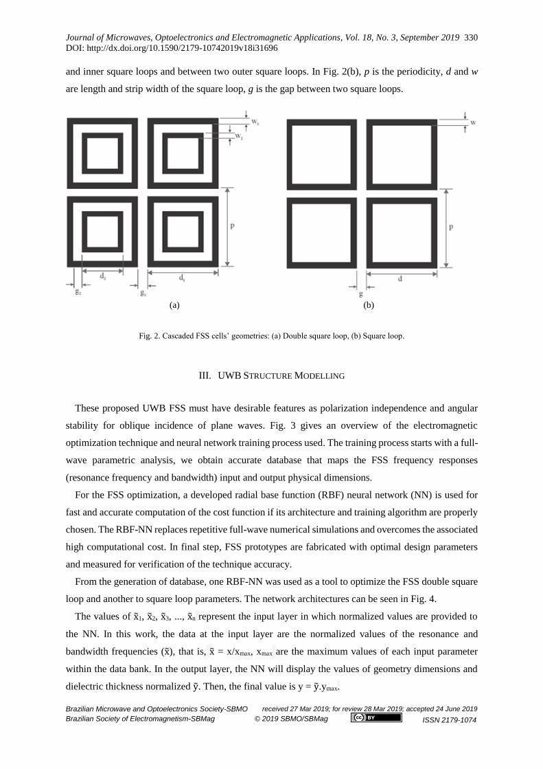
Fig. 2 illustrates the cells’ geometries. Fig. 2(a) illustrates the double square loop geometry used in

FSS1 and its parameters. Fig. 2(b) illustrates the square loop geometry used in FSS2 and its parameters.

In Fig, 2(a), p is the periodicity, d1 and w1 are length and strip width of the outer square loop; d2 and

w2 are length and strip width of the inner square loop. g2 and g1 are, respectively, the gap between outer





330

and inner square loops and between two outer square loops. In Fig. 2(b), p is the periodicity, d and w

are length and strip width of the square loop, g is the gap between two square loops.

(a) (b)

Fig. 2. Cascaded FSS cells’ geometries: (a) Double square loop, (b) Square loop.

III. UWB STRUCTURE MODELLING

These proposed UWB FSS must have desirable features as polarization independence and angular

stability for oblique incidence of plane waves. Fig. 3 gives an overview of the electromagnetic

optimization technique and neural network training process used. The training process starts with a full-

wave parametric analysis, we obtain accurate database that maps the FSS frequency responses

(resonance frequency and bandwidth) input and output physical dimensions.

For the FSS optimization, a developed radial base function (RBF) neural network (NN) is used for

fast and accurate computation of the cost function if its architecture and training algorithm are properly

chosen. The RBF-NN replaces repetitive full-wave numerical simulations and overcomes the associated

high computational cost. In final step, FSS prototypes are fabricated with optimal design parameters

and measured for verification of the technique accuracy.

From the generation of database, one RBF-NN was used as a tool to optimize the FSS double square

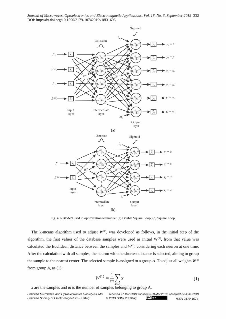
loop and another to square loop parameters. The network architectures can be seen in Fig. 4.

The values of x1, x2, x3, ..., xn represent the input layer in which normalized values are provided to

the NN. In this work, the data at the input layer are the normalized values of the resonance and

bandwidth frequencies (x), that is, x = x/xmax, xmax are the maximum values of each input parameter

within the data bank. In the output layer, the NN will display the values of geometry dimensions and

dielectric thickness normalized y. Then, the final value is y = y.ymax.





331

Fig. 3. Overview of optimization technique and neural network training.

In order, to be able to learn the NN two steps are required: training and validation. The training of

the NN consists of adjusting the values of the weights W(1) and W(2), which are the synaptic weights of

the connections between the entry and the intermediate layer and, from the intermediate layer to the

output layer, respectively. With the adjustment of the weights, the NN extracts the characteristics of the

database and has generalization capacity. In the middle layer of proposed NN, whose learning occurs

unattended, the activation function is a Gaussian type. Gaussian function is commonly used as the radial

basis in RBF neural network.

The method of adjusting the weights W(1), a unsupervised learning, was used k-means [14]. K-means

algorithm is a kind of cluster algorithm, it was proposed by J. B. MacQueen [15]. The main aim of k-

means is to position k-Gaussian centers in regions where input patterns will tend to cluster. The centers

are represented by the synaptic weights (W(1)) of the NN and the variance of each Gaussian activation

functions was calculated by the criterion of the mean square distance.





332

(a)

(b)

Fig. 4. RBF-NN used in optimization technique: (a) Double Square Loop; (b) Square Loop.

The k-means algorithm used to adjust W(1), was developed as follows, in the initial step of the

algorithm, the first values of the database samples were used as initial W(1), from that value was

calculated the Euclidean distance between the samples and W(1), considering each neuron at one time.

After the calculation with all samples, the neuron with the shortest distance is selected, aiming to group

the sample to the nearest center. The selected sample is assigned to a group A. To adjust all weights W(1)

from group A, as (1):

𝑊(1) =1

𝑚∑ 𝑥𝑥∈𝐴

(1)

x are the samples and m is the number of samples belonging to group A.





333

This instruction is repeated until there are no more changes in group A between the interactions.

After this, the variance of each of the Gaussian activation functions is calculated by the criterion of

the mean square distance, according to (2).

𝜎2 =1

𝑚∑∑(𝑥 −𝑊(1))

2

𝑥∈𝐴

(2)

In the output layer, the weights W(2) are adjusted after the intermediate layer, and for its adjustment

was used the learning algorithm that implements the generalized delta rule, whose objective, in a

supervised way, is to minimize the error mean square given in (3):

𝑀𝑆𝐸 =1

𝑞∑𝐸(𝑖)

𝑞

𝑖=1

(3)

where E(i) is the quadratic error consisting of the difference between the desired value and the response

of the output layer for each sample i, and q is the number of samples at one time. E(i) is:

𝐸(𝑖) =1

2∑(𝑑𝑛(𝑖) − 𝑦𝑛(𝑖))

2

𝑛2

𝑛=1

(4)

where dn(i) is the nth desired response and yn(i) is the nth NN output.

The activation function used in neurons of the output layer was the sigmoid function. This function

was the first to be tested in the network, because it is computationally easy to perform, as it obtained

good results, no other was tested.

As a criterion of stopping, the mean square error (MSE) to be reached was used. When the MSE

reached and the MSE of validation differentiated by 20%, it was considered that the neural network

converged and the process ended, or if the neural network doesn’t converge after 200,000 epochs.

To train and validate the neural networks to optimize the parameters of square loop FSS and double

square loop FSS, a database was generated with the parameters described in Table 1 and Table 2. To

extract the values of resonance frequency and bandwidth it was utilized ANSYS HFSS software. And

all simulations were performed a range of frequency of 1 to 40 GHz. And the substrate utilized was

FR4.

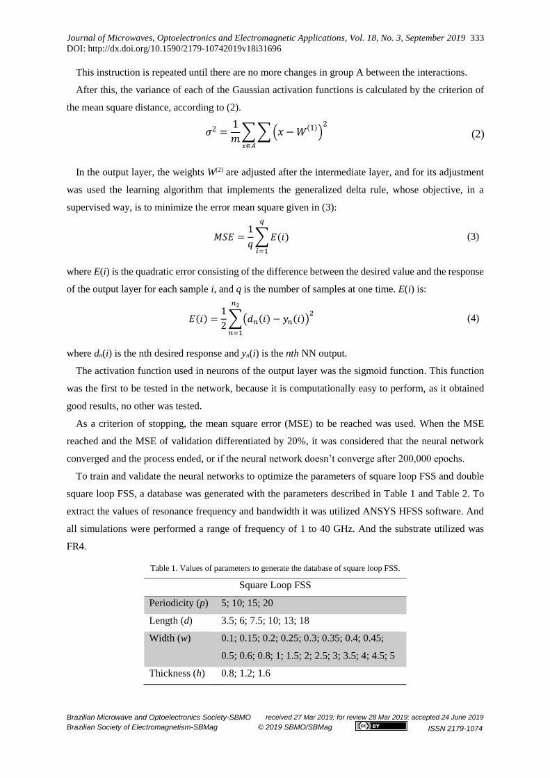
Table 1. Values of parameters to generate the database of square loop FSS.

Square Loop FSS

Periodicity (p) 5; 10; 15; 20

Length (d) 3.5; 6; 7.5; 10; 13; 18

Width (w) 0.1; 0.15; 0.2; 0.25; 0.3; 0.35; 0.4; 0.45;

0.5; 0.6; 0.8; 1; 1.5; 2; 2.5; 3; 3.5; 4; 4.5; 5

Thickness (h) 0.8; 1.2; 1.6





334

Not all combinations of Table 1 are possible, and the database was composed only of the samples

that presented one resonance frequency. The database was formed by 104 samples.

To optimize square loop FSS, the resonance frequency and bandwidth values are presented in the

input layer (x), whose maximum values (xmax) were 21 GHz and 10.5 GHz, respectively. At the output

(y), the values of d, p, w and h, whose maximum values (ymax) were: 18 mm, 20 mm, 5 mm and 1.6 mm,

respectively.

For the training of NN from the database generated by the FSS with square loop geometry, were

inserted: 2 neurons in the input layer that correspond to the resonance frequency and bandwidth; 36

neurons in the hidden layer and 4 neurons in the output layer that correspond to the constructive

parameters of the square loop geometry. The number of neurons in the middle layer in each NN was

adjusted from the minimum number of epochs to arrive at the required mean square error in training.

In the NN training, it was noticed that the learning rate of 0.006 and the mean square error to be

reached equal to 0.05 in training stage were sufficient for the network to perform the FSS optimization

at the desired frequency and bandwidth in the project. 80% of the data were used for training and the

rest was used for validation. The test of NN was realized with project parameters, as seem in Table 3.

Fig. 5 shows the training and validation results for the RBF-NN. The NN reach the aim around 50,000

epochs.

Fig. 5. Training and validation of NN for FSS with square loop geometry.

In the generation of the database for training and validation of neural network, the FSS parameters

d1, d2, p, w1, w2 and h were varied according to Table 2.

Not all combinations of Table 2 are possible, and the database was composed only of the samples

that presented double band response. The database was formed by 287 samples.





335

Table 2. Values of parameters to generate the database of double square loop FSS.

Double Square Loop FSS

Parameters Values (mm)

Periodicity (p) 5; 10; 12; 15; 16; 20.

Length (d1) 4.5; 7; 7.5; 8; 9; 9.6; 10.2; 11.5; 12; 13; 15; 1.

Width (w1) 0.1; 0.15; 0.2; 0.25; 0.3; 0.35; 0.4; 0.5; 0.6; 1;

1.5; 2; 2.5; 3.

Length (d2) 2,5; 5; 6,5; 7; 7,2; 8; 9; 12; 15;

Width (w2) 0.1; 0.15; 0.2; 0.25; 0.3; 0.35; 0.4; 0.5; 0.6; 1;

1.5; 2; 2.5; 3; 3.5; 4

Thickness (h) 0.8; 1.2; 1.6.

For the optimization of the double square loop, the values of the resonance frequency of the first band

(fr1) and its bandwidth (BW1), the resonance frequency of the second band (fr2) and its bandwidth (BW2)

are presented to the network input (x), whose maximum values (xmax) were: 18 GHz, 5.5 GHz, 45 GHz

and 8 GHz, respectively. At the output (y), the values of d1, d2, p, w1, w2 and h, whose maximum values

(ymax) are: 19 mm, 15 mm, 20 mm, 3 mm, 4 mm and 1.6 mm.

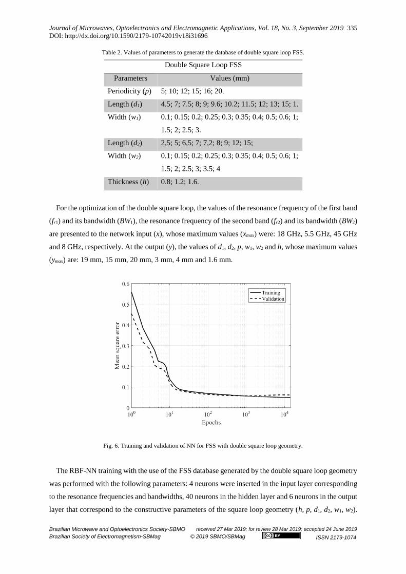
Fig. 6. Training and validation of NN for FSS with double square loop geometry.

The RBF-NN training with the use of the FSS database generated by the double square loop geometry

was performed with the following parameters: 4 neurons were inserted in the input layer corresponding

to the resonance frequencies and bandwidths, 40 neurons in the hidden layer and 6 neurons in the output

layer that correspond to the constructive parameters of the square loop geometry (h, p, d1, d2, w1, w2).





336

Learning rate was 0.1, the mean square error to be reached was 0.05 in training stage and the evolution

of the network in its training and validation can be visualized in Fig. 6. 80% of the data were used for

training and the rest was used for validation. The test of NN was realized with project parameters, as

seem in Table 4. The NN reach the aim around 14,000 epochs.

In the NN trained with the square loop database, was entered the input parameters: resonance

frequency and bandwidth and, as output parameters, we found the values for the optimized FSS, as

visualized in Table 3.

Table 3. Square loop optimized.

Square Loop Design (FSS 2)

Input Parameters

fr BW

5.8 GHz 3.0 GHz

Output Parameters

h p D W

1.2 mm 12.6749 mm 11.0918 mm 1.2874 mm

The same procedure was performed for the NN trained with the double square loop database. The

input parameters: resonance frequency and bandwidth and the output parameters were the optimized

values of the FSS, according to Table 4.

Table 4. Double square loop optimized.

Double Square Loop Design (FSS 1)

Input Parameters

fr1 BW1 fr2 BW2

3.0 GHz 1.5 GHz 9.0 GHz 3.0 GHz

Output Parameters

h P d1 d2 w1 w2

1.2 mm 12.6749 mm 12.1712 mm 8.4438 mm 0.4268 mm 1.1075 mm

IV. NUMERICAL AND EXPERIMENTAL RESULTS

After modeling with the RBF-NN the physical dimensions necessary to obtain the desired frequency

responses for the two proposed structures, FSS1 and FSS2, simulations of the transmission

characteristics of these structures were done in the ANSYS HFSS software. Fig. 7 illustrates these

simulations. The gray areas are the desired bandwidths. For FSS1, simulations obtain BW = 2.84 GHz

and fr = 6.0 GHz, very close to desired values (Table 3). For FSS2, simulations obtain BW1 = 1.23 GHz,

fr1 = 3.2 GHz and BW2 = 2.74 GHz and fr2 = 9.1 GHz, also very close to desired values (Table 4). So,

bandwidth and resonant frequency requirements met. Differences did not reach 10 %.





337

After the design of the isolated FSS, we performed a parametric study to find the best distance (air

gap) between cascaded FSS (Fig. 1). In this study, we varied the gap value from 0 to 30 mm. After this

parametric analysis, we realized that an ultra-wide bandwidth would be possible with the gap value of

5 mm. Thus, we cascaded the two FSS and simulated the structure in the ANSYS HFSS software. The

results can be seen on Fig. 8. Considering |S11| = – 10 dB, bandwidth obtained was 7.6 GHz (3.05 –

10.65 GHz), sufficient for UWB, that is 7.5 GHz (3.10 – 10.60 GHz). So, simulations show that our

proposed cascaded FSS can be used in UWB applications.

Fig. 7. Simulated results for frequency response of the FSS1 (——) and FSS2 (- - - - -).

Fig. 8. Simulated results for the cascaded structure.

It is also important that the cascaded structure has polarization independence and angular stability.

So, we simulated the transmission characteristic for vertical and horizontal polarization and for different

angles of incidence. In Fig. 9, we can see the frequency response of the FSS designed for vertical

polarization. The incident angles are changed from 0 to 30 degrees; this is because our setup

measurement has no capability to measure bigger angles. It may be noted that, for our frequency range





338

of interest, there is no degradation in bandwidth. This shows that the geometry is stable in terms of

incidence angles, for vertical polarization.

In Fig. 10 we can see the frequency response of the FSS designed for different angles of incidence

and horizontal polarization. It may be noted that, although some degradation has occurred near 9 GHz,

this degradation does not exceed – 10 dB, for the |S11|, maintaining the performance of the structure, as

in the case of vertical polarization. This shows that the structure has polarization independence and

angular stability.

Fig. 9. Simulated results for oblique incidence and vertical polarization.

Fig. 10. Simulated results for oblique incidence and horizontal polarization.

To validate the analysis performed, prototypes were built and experimental characterizations were

performed. Thus, we could compare the simulated results with measurements. The measurements were

carried out using a vector network analyzer (VNA) from Agilent, model E5071C, two horn antennas of

the manufacturer A. H. Systems, model SAS-571 (700 MHz to 18 GHz), positioned in direct line of

sight. A photograph of measurement setup and of device under test (DUT) is shown in Fig. 11. The

absorber is used to avoid diffraction around the edges of the panel. For fabrication purposes, the





339

dimensions provided by the RBF-NN must be truncated. So, for FSS1 the dimensions used in fabrication

were: h = 1.2 mm; p = 12.7 mm; d1 = 12.2 mm; d2 = 8.4 mm; w1 = 0.4 mm; and w2 = 1.1 mm. For FSS2

the dimensions used in fabrication were: h = 1.2 mm; p = 12.7 mm; d = 11.1 mm and w = 1.3 mm.

Fig. 11. Measurement setup.

Fig. 12 illustrates the cascade FSS, with plastic spacers and screws.

Fig. 12. Cascade FSS.

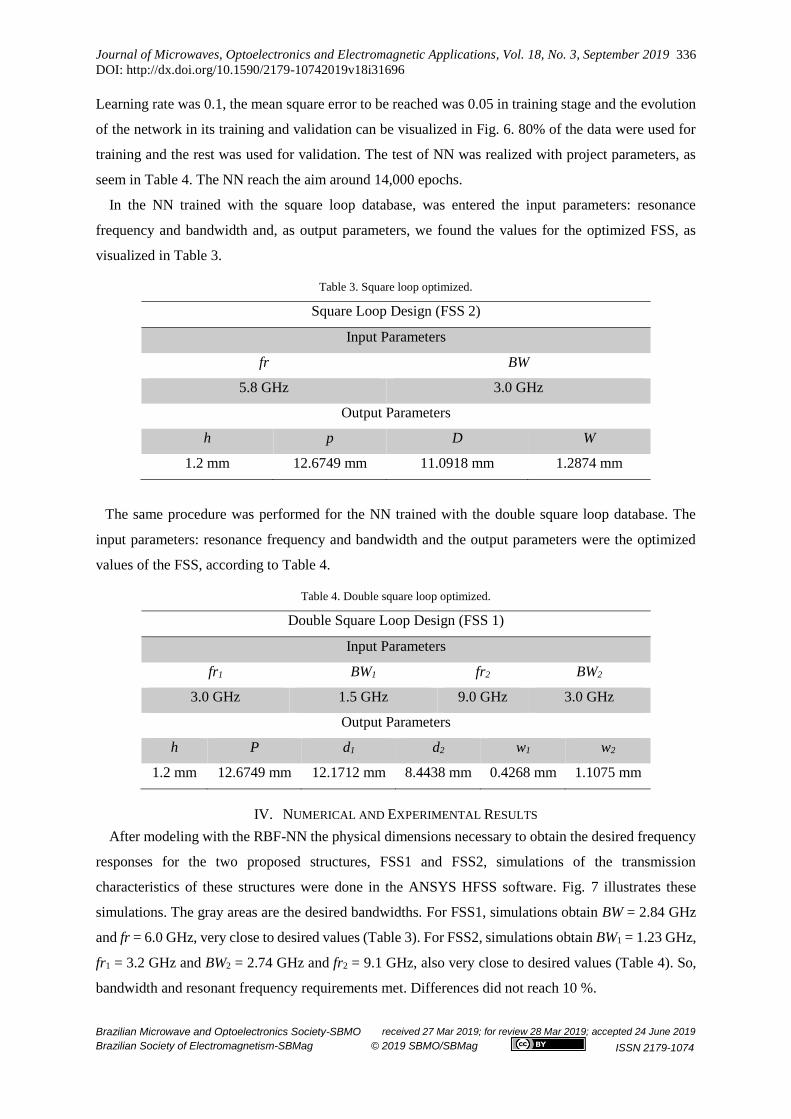
In Fig. 13 we can see a comparison between numerical and measured results for FSS1 for normal

incidence. Desired results were: fr1 = 3.0 GHz and BW1 = 1.5 GHz; fr2 = 9.0 GHz and BW2 = 3.0 GHz.

Simulated results were: fr1 = 3.25 GHz and BW1 = 1.18 GHz; fr2 = 9.13 GHz and BW2 = 2.51 GHz.

Measured results were: fr1 = 3.46 GHz and BW1 = 1.49 GHz; fr2 = 9.68 GHz and BW2 = 3.66 GHz. The

measured and simulated results show good agreement. The main difference is due to the truncation on

physical dimensions because the limitation of manufacture.





340

Fig. 13. Comparison between simulated and measured results for FSS1.

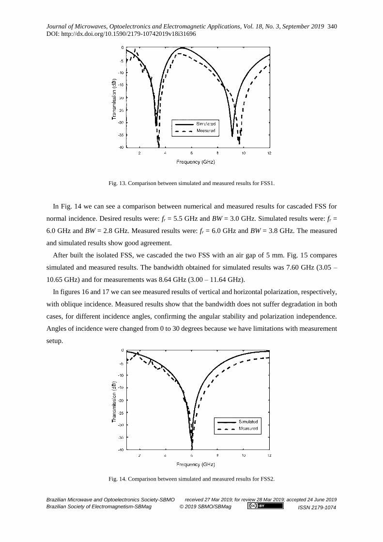
In Fig. 14 we can see a comparison between numerical and measured results for cascaded FSS for

normal incidence. Desired results were: fr = 5.5 GHz and BW = 3.0 GHz. Simulated results were: fr =

6.0 GHz and BW = 2.8 GHz. Measured results were: fr = 6.0 GHz and BW = 3.8 GHz. The measured

and simulated results show good agreement.

After built the isolated FSS, we cascaded the two FSS with an air gap of 5 mm. Fig. 15 compares

simulated and measured results. The bandwidth obtained for simulated results was 7.60 GHz (3.05 –

10.65 GHz) and for measurements was 8.64 GHz (3.00 – 11.64 GHz).

In figures 16 and 17 we can see measured results of vertical and horizontal polarization, respectively,

with oblique incidence. Measured results show that the bandwidth does not suffer degradation in both

cases, for different incidence angles, confirming the angular stability and polarization independence.

Angles of incidence were changed from 0 to 30 degrees because we have limitations with measurement

setup.

Fig. 14. Comparison between simulated and measured results for FSS2.





341

Fig. 15. Comparison between simulated and measured results for cascaded structure.

Fig. 16. Measured results for oblique incidence and vertical polarization.

Fig. 17. Measured results for oblique incidence and horizontal polarization.





342

V. CONCLUSIONS

In this article we proposed a structure formed by two cascaded FSS to obtain UWB frequency

response. The geometries chosen for the FSS design were the double square loop and the square loop,

since both have good angular stability and polarization independence. Computational intelligence tools

were used to optimize the FSS design, reducing the time and computational effort of the project. The

cascade technique was chosen because it proved efficient in other studies [13]. The final structure

obtained a stop-band response across the UWB frequency range (3.1 – 10.6 GHz), and can be used in

different applications, such as microstrip antenna optimization. To validate the analysis performed

prototypes were fabricated and measurements were performed. A good agreement between numerical

and experimental results was observed. The experimental results proved the UWB response, the

polarization independence and the angular stability of the structure.

ACKNOWLEDGMENT

The authors express their sincere thanks to National Council of Research and Development – CNPq

for supporting the research work over the project 303693/2014-2.

REFERENCES

[1] B. A. Munk, Frequency selective surfaces: Theory and design, New York, NY, Wiley, 2000.

[2] H. B. Baskey and M. J. Akhtar, “Design of flexible hybrid nanocomposite structure based on frequency selective surface

for wideband radar cross section reduction”, IEEE Transactions on Microwave Theory and Techniques, Vol. 65, No. 6,

pp. 2019–2029, 2017.

[3] J. C. Zhang, Y. Z. Yin, and J. P. Ma, “Design of narrow band-pass frequency selective surfaces for millimeter wave

applications”, Progress in Electromagnetics Research, Vol. 96, No. 4, pp. 287–298, 2009.

[4] M. Sharifian and M. Mollaei, “Narrow-band configurable polarization rotator using frequency selective surface based on

circular substrate integrated waveguide cavity”, IEEE Antennas & Wireless Propagation Letters, Vol. 16, pp. 1923–1926,

2017.

[5] J. Lorenzo, A. Lazaro, D. Girbau, R. Villarino, and E. Gil, “Analysis of on-body transponders based on frequency

selective surfaces”, Progress in Electromagnetics Research, Vol. 157, pp. 133–143, 2016.

[6] J. Tiemann, F. Schweikowski, and C. Wietfeld, “Design of an UWB indoor-positioning system for UAV navigation in

GNSS-denied environments”, IEEE International Conference on Indoor Positioning and Indoor Navigation, 2015.

[7] G. Izabela, L. Vinay, G. Leonid, A. Donald, and B. Frank, “Analyses and simulations for aeronautical mobile airport

communications system”, Integrated Communications Navigation and Surveillance, 2016.

[8] J. Wang, G. Guo, and H. Zheng, “Characteristic analysis of nose radome by aperture-integration and surface-integration

method”, IEEE International Workshop on Microwave and Millimeter Wave Circuits and System Technology, 2012.

[9] H. Zhou, S. B. Qu, and J. F. Wang, “Ultra-wideband frequency selective surface”, Electronics Letters, Vol. 48, No. 1, pp.

11–13, 2012.

[10] S. Ramprabhu, M. Balaji, and K. Malathi, “Polarization-independent single-layer ultra-wideband frequency-selective

surface”, Journal of Electromagnetic Waves and Applications, Vol. 9, No. 1, pp. 93–97, 2015.

[11] B. Hua, X. Liu, X. He, and Y. Yang, “Wide-Angle Frequency Selective Surface with Ultra-Wideband Response for

Aircraft Stealth Designs”, Progress in Electromagnetics Research C, Vol. 77, pp. 167–173, 2017.

[12] A. Chatterjee and S. K. Parui, “A Dual Layer Frequency Selective Surface Reflector for Wideband Applications”,

Radioengineering, Vol. 25, No. 1, 2016, pp. 67 – 72.

[13] F. C. G. da Silva Segundo, A. L. P. S. Campos, and A. Gomes Neto, "A design proposal for ultrawide band frequency

selective surface", Vol. 12, no. 2, Journal of Microwaves, Optoelectronics and Electromagnetic Applications, pp. 398 -

409, 2013.

[14] Zhenxiang Xing, Hao Guo, Shuhua Dong, Qiang Fu, Jing Li, “RBF Neural Network Based on K-means Algorithm with

Density Parameter and Its Application to the Rainfall Forecasting”, 8th International Conference on Computer and

Computing Technologies in Agriculture (CCTA), Sep 2014, Beijing, China.

[15] Youguo Li, Haiyan Wu, “A clustering method based on K-means Algorithm”, International Conference on Solid State

Devices and Materials Science, pp. 1104-1109, 2012.

double layer frequency selective surface for ultra wide

Documents