double helical ensemble multi-dimensional 4-d structured

6447

Turkish Journal of Computer and Mathematics Education Vol.12 No.13 (2021), 6447 - 6458

Double Helical Ensemble Multi-Dimensional 4-D Structured Neural Network to Analyze the Driving Pattern, Driver DNA and Generate License Score using Smartphone Sensor Data

Dr. S. Karthikeyana, Dr. S. Gopikrishnana, Dhruv Battaa and TathagatBanerjeea

aSchool of Computer Science and Engineering, VIT-AP University, Amaravati, Andhra Pradesh, India.

Article History: Do not touch during review process(xxxx)

_____________________________________________________________________________________________________

Abstract: In this paper, we delineate a way to assess the licensed score of a person. License score is a term coined here in reference with a credit score which is used to identify the credibility of an individual on a financial basis. This research leverages the accelerometer and gyroscope sensors present in the smartphones. These sensors help us realize our goal of classifying driving events and detecting distracted driving due to the use of smartphones. We use sensors rich user micro

movements and irregularities that can be detected by sensors in the phone during driving. Our system distinguishes driving events based on reference signals which are matched through our Pattern Matching Algorithm which uses dynamic time warping. To validate our approach, we conducted extensive experiments with several users on various vehicles and

smartphones. A neural network model has been developed for the purpose of classifying signals in the future which leverages our collected data. The model has a double helical stranded multidimensional 4-d neural network that uses layers of Convolutional Neural Networks and Artificial Neural Networks. It uses long short-term memory (LSTM) layers to classify and score the driving behaviours. The double-helical stranded neural network simulates a situation similar to the input and output

of different senses of the human brain. This helps us classifying driving events.

Keywords: Accelerometer; Gyroscope; Pattern Matching; Dynamic Time Warping; Convolutional Neural Networks; Artificial Neural Networks; Helical; LSTM; Credit Score

___________________________________________________________________________ 1. Introduction

The automobile industry has increased dramatically over the last two decades. In India, the growth itself has

seen an increase of an astounding 7.08 percent per year. According to IBEF, India has produced 29.07 million

vehicles in the financial year 2018. With the ever-increasing need of transport, automobile industry has flourished

in recent years. This amelioration for the automobile industry has come with a cost that no nation wants to bear. In

the last decade or so, the amount of road accidents has significantly increased. Road accidents have become the

leading cause of deaths due to injuries and are the tenth leading cause of deaths all over the world. An estimated

1.2 million people are killed in road crashes each year, and as many as 50 million are injured, occupying 30

percent to 70 percent of orthopedic beds in developing countries hospitals. If present trends continue, road traffic

injuries are predicted to be the third-leading contributor to the global burden of disease and injury by 2020. This is

a huge burden not only human resource-wise but also financially for countries. Since most countries provide

healthcare insurance and automobile insurance. Paying for the costs of damage done due to accidents and then as

these numbers rise so does the basic premium cost for the insurance. These increased premium costs are to be paid

by everyone irrespective of how safely or rashly they drive. With this, the automobile insurance industry has been

rapidly transitioning from traditional fixed fee insurance packages to usage-based insurance. We believe that the

majority of well-behaved drivers should not have to pay more for others’ faux pass.

We developed a sophisticated scoring algorithm that allows us to leverage smartphone sensors to overcome

Blackbox costing operations and define the driver’s behavior (Good, Bad, and Average). Smartphones contain the

exact same sensors as those in Black boxes, namely accelerometer, gyroscope, magnetometer, and GPS sensors.

These sensors are calibrated and used so that results remain in the same range for different smartphones and in

different cars.In this paper, we aim not only to diagnose the traffic insight, anticipation and behavior of driver

while driving but also provide a better basis for usage-based insurance and ensure that the financial burden

decreases and the number of road accidents come down through self-analysis.

Research Article

Dr. S. Karthikeyan, Dr. S. Gopikrishnan, Dhruv Batta and Rohit Bhargav Peesa

6448

2.Review of Related Studies

Numerous innovative systems in addition to system designs have been proposed and developed in the past to

detection of drivers, detect drowsiness of driver, prevent usage of cell phones by drivers, driver distractions, driver

fatigue and to detect many other activities. The number of road accidents happening has been increasing day by

day. One of the major causes is either drunk and drive or drowsiness. H. Singh et al. have designed a non-intrusive

system (Singh.et al.,2017)which constantly monitors driver’s eyes and can detect fatigue of the driver

subsequently it generates timely warnings in the form of sound and seatbelt vibrations which helps in preventing

road accidents. The system is designed to deactivate warnings manually rather than automatically so that the

driver becomes alert. There are chances that driver may feel drowsy and sudden press accelerator or brake which

can cause accidents and to prevent this they plot a graph in the time domain and when all the three input variables show a possibility of fatigue at that moment then warning signal would be activated and given as red-colored

circle or text.

Doshi, Anup et al.have proposed a driving behavior analysis method based on the vehicle onboard diagnostic

information and Adaboost algorithm(Doshi. et al., 2015). The method makes use of Adaboost algorithm to create

driving behavior classifier based on inputs collected namely speed, RPM, engine load and throttle position through onboard diagnostic interface setup. The classifier model with an accuracy rate of 99.8 percent is used to

classify whether the driver's behavior is safe or not.P. Hermannstädter and B. Yang have proposed a model which

can describe driver behavior by means control theoretic driver models(Hermannstädter. et al., 2013). They have

applied a driver model to real-road driving where they assessed the driver’s state i.e. distracted or not. Model

parameters have been estimated by means of prediction error identification on data of eleven different drivers

They evaluate the distributions of the driver model parameters and the predictive capability of the estimated driver

models. These evaluated distributions along with estimated model parameters play a vital role in estimating

distracted drivers’ behavior which proves that model parameter and predictive performance can affect the output.

Real-time system for monitoring driver vigilance is a paper by Bergasa et al.(Bergasa. et al., 2006) where the

authors proposed a feasible prototype to detect driver’s distraction using wearable equipment which consists of

cameras to monitor driver’s vigilance in real-time. Kutila et al. (Kutila. et al., 2007) have proposed Driver

distraction detection with a camera vision system where they developed another smart human-machine interface to

measure the driver’s momentary state by fusing stereo vision and lane tracking data. These two approaches were

successful in attaining accuracy of 77 per cent at an average but they do are not considered as a handheld device.

Salvucci (Salvucci. et al., 2001) proposed a cognitive architecture to predict the effects of the in-car interface on

driver’s behavior based on a cell phone. All the above-mentioned systems require modifications to the car which

would increase the cost and causes complexities in coordination in between components of the system. There are

few alternatives designed to overcome the issues above. One major alternative is Yang et al. (Youssef. et al.,

2010) proposed an innovative method with the help of connectivity between smartphone and car through

Bluetooth connection in the car's stereo system. This model locates the phone with the help of the relative delay

between the signal sent from speakers. Even this system had issues since old cars were not equipped with

Bluetooth. Moreover, the cabin sizes and Bluetooth configurations were varying from car to car and phone to

phone which was a cause that affected the accuracy of the system. Chu et al.(Bao. et al., 2004)proposed a similar

system which is a phone-based sensing system to determine whether the user is a driver or passenger without

depending on multiple additional wearable sensors or modifications to the car. This model simply depends on the

collaboration of multiple phones which are used to process in-car noises. Later, these inputs are used in a back-end

cloud service to differentiate between a passenger and a driver.

Our approach involves numerous activity detections and recognitions using sensors integrated in smartphones

inspired from various existing techniques being used in papers mentioned further.Ravi et al.(Ravi. et al., 2008)

proposed a system which recognizes motion activities with the help of data collected from HP iPAQ which is used

to collect data wirelessly. Lee et al.(Lee. et al., 2002)presented a system to identify the user's location and

activities through accelerometers and angular velocity sensors in the pocket along with a compass on the waist.

Bao et al.(Bao. et al., 2004) has introduced a technique for activity recognition based on multiple accelerometer

sensors positioned in various body parts such as arms, wrists, ankles and so on. The process of understanding driver’s behavior is becoming a task of interest presently so as to train autonomous applications and determining

accidental risks. Umberto Fugiglando et al. have proposed a new concept called Driver DNA(Fugiglando. et al.,

2017)where characterization of driver’s behavior is done through four different easy-to-measure factors, called

DNA dimensions which is an easier way to describe the complexity of driving behavior. It is estimated for each

driver and assigned a synthetic score, which is a unique representation of specific driver’s driving skills. The four

dimensions namely driving, comfort,accident risk and fuel efficiency are a result of the process of analysis of

database. It is efficient when compared to regular machine learning techniques due to low computing complexity

and skills are characterized which makes it easier to compare driving’s’ of various drivers. Moreover, these DNA

dimensions can be visualized on car’s dashboard which lets the driver understand his driving issues and influences

him to modify it.

Double Helical Ensemble Multi-Dimensional 4-D Structured Neural Network

6449

Sentience has developed a platform that makes use of sensors in smartphones namely accelerometer,

gyroscope, magnetometer and GPS sensors. Algorithm has been developed along with machine learning

techniques to be adaptable to phone’s sensor characteristics, road types and so on. Smartphones sensors data are

being used to make model to differentiate phone handling on how it moves while driving. This model has attained

an AUC score of 96 percent. To compare and analyze specific user’s driving experience they have made use of

scores namely efficiency, anticipation, phone usage while driving, legalese i.e.speeds limits, traffic violations etc.

3. Proposed Methodology

In our research, we have designed our experiments and our data acquisition in a peculiar manner. Through the

data acquired from the experiments, we have found thresholds of various behaviours of a driver while driving their

car. Based on your driving aggressiveness, traffic insight and anticipation, and speeding behaviour, costs of

premium can be adapted to the individual. To categorize drivers driving style (Good, Bad, and Average), We

planned to track following parameters:

Frequent braking

Hard/Aggressive braking

Hard/Aggressive forward acceleration

Hard/Aggressive turns

Sudden Turns

Hard Braking

Hard Acceleration

Lane change (not accompanied by indicator sound)

Sudden lane change

Speed too high for the curve

Rainy curve

Speed Limit Violation

Distracted driving/Phone Usage/Texting/Talking on phone

Our experiments for research was based on the following structure

Socket: for sensors connection and data fetching from the mobile end.

Machine Learning (Python, TensorFlow, Sci-kit Learn, Keras)

3.1 Socket:

We used the socket to communicate with the device(smartphone) in real time. We have a use-case pf how to

detect the user in real time if he/she has started driving or not, Because of that we need the accelerometer data in

real time to detected that he started driving or not. If we found the user has moved, we create his trips and record

the sensors data for ML Process.

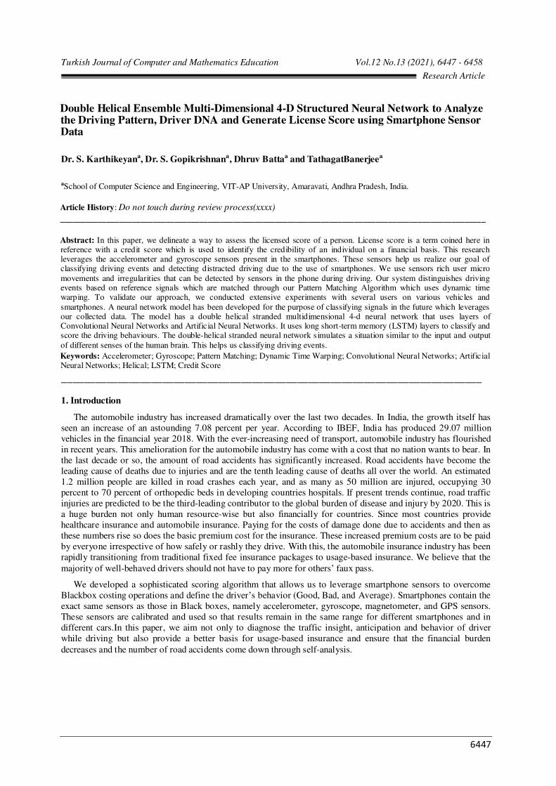
Now, we discuss the methodology how we handle each and every use case of the user and how what does

socket’s mechanism do with the data from a smartphone. This is depicted in Fig.2.

Algorithm:

Step 1: Read the sensor data through the heartbeat socket. Get the value of ‘User ID’ and Speed.

Step 2: Check the speed, if the value is greater than 4 then go to step 3 else go to step 4.

Step 3: Find the trip of the user where finished is equal to zero. If we find the record that means previous trips

is running else create new trip.

Step 4: Find the running trips from the database, if no record exists return ‘user in ideal state’ else find the

sensor data from the database using the trip id and find the last moving record and compare the timestamp with

current timestamp and go to step 5.

Step 5: If comparison is greater than 5 minutes then the trip ends else return user in traffic state.

3.2 Data Pre-Processing:

Requirements:

Accelerometer data (x, y, z)

Gyroscope Data (x, y, z)

Vehicle Speed

GPS Data


6450

Compass Data

Magnetometer Data

3.2 Data Reformatting

Data Transform : Gather the collected data from the experiment and the events with the sensors data

(mentioned in the above example) and transform the data with the help of min- max scalar which can convert all

the big numbers and small numbers into a single unit between -1 to 1, which is much easier for the calculation

and efficiency.

Create Sliding Window: After Data is transformed, we created a sliding window for each second to detect

events. So now, after the sliding window is created it will return the data into batches.

Calculate Mean Median Mode: We can calculate the mean, median, mode for each sliding window with

batches and clear the data distortion and noise errors of the sensor data.

Driving Events: After clearing the distortion and noise errors we assigned the driving events to the patterns

observed in the data.

Using Dynamic Time Warping Algorithm with Pattern Recognition Algorithm. The pattern matching

algorithm uses data from accelerometer sensor in the phones. The accelerometer sensor is free from external

factors that create a limitation on the missing data set. Since, all data is recorded through the sensors on the

phone.The accelerometer and gyroscope provide measurements to the socket in 3-axis domain, vertical,

longitudinal and lateral. Data from all sensors is recorded at a rate of 10Hz in this work in order to form a time

series of acceleration, gyroscope and magnetometer. The following pattern matching algorithm which is different

than the one presented in another research which uses pattern recognition.

This is based on the Dynamic Time Warping (DTW) technique. Dynamic Time Warping is used to find

patterns in time series of the sensor data’s batches formed and the frequency at which they were acquired.In

general, Dynamic Time Warping technique provides a similarity measure between two signals, namely the

incoming and the reference signals. The main feature of this technique is that it allows for stretched and

compressed portions of the two signals to be compared by compensating for length differences in the two signals

while considering the non-linearity of the length differences between the incoming signal and the reference

signal. This feature is not possible with a traditional pairwise comparison between the two signals using the

Euclidean distance.

Pattern Matching: This is the stage where DTW algorithm is deployed to find the best match using a given

reference pattern for all driver actions. The primary goal in this stage of the algorithm is to use the experimented

driving patterns to find an appropriate match for the incoming driving data. In order to generate appropriate

reference patterns, for each driver action, a training data set is obtained through our real-world experiments on 60

drivers over 6000 trips. From our pattern matching algorithm, these reference patterns are then used as a threshold

to match the incoming signals from sensors in the test data set. In this paper, 70% of data samples are utilized as

training data, resulting in 30% to be used as test data set. At the completion of the algorithm, a total cost of the

alignment path is obtained for all of the thresholds selected to cover all the described actions. Fig.1 describes how

an optimal alignment path can be found and its cost calculated.

Figure.1. (a) Optical alignment path and (b) cost estimation

Figure.2. Proposed Methodology


6451

3.3 Batch Normalization

The acceleration and gyroscope sensor values are stored in window batches and a slider is attached which

increases as pertaining to a number of records present in the data. These are then normalized in a TensorFlow

session. The batches which were made, we used the median of each batch and stored all the six features median in a data frame.

Pattern Creation and Matching

The reference signal pattern can be seen in the following image: -


6452

All the peaks in acceleration Y, showcase change in acceleration in the Y domain. This domain is responsible

for sensing jerky actions of car such as hard acceleration and hard braking; which might cause a change in inertia

of the phone. This goes on to show that we can use acceleration in Y domain as a parameter to label an event as

hard acceleration and hard braking. The difference between these two can be found as we check with acceleration

in Z domain since Acceleration in Z is one of the main parameters for finding threshold of hard braking and hard

acceleration in the interpolated data. A large trough included in the plot of acceleration Z indicates presence of

Hard Breaking while a peak suggests hard acceleration.

All the peaks in Gyro Y, showcase change in the sensor values when there is a sudden turn. This domain is

responsible for sensing sudden change in actions of car such as aggressive right or left turn; which might cause a

change in orientation of the phone. This goes on to show that we can use gyro in Y domain as a parameter to label

an event as sudden turn and rainy curve. The difference between these two can be found as we check with

gyroscope in Y domain since gyroscope in this domain is one of the main parameters for finding threshold of

sudden turns in the interpolated data. A large peak included in the plot of Gyro X indicates presence of a sudden

turn made while a peak suggests sudden turn or rainy curve.After we have found thresholds for the values, then

we combine the graphs so as to understand how the values at a certain event vary with respect to other values.

1. Speed Limit Violation:

Step 1: Get the moving vehicle speed (Calculate the Speed of the vehicle with the help of GPS data)find

the variation in the lat-long and calculate the speed in meters per second. (Provided by Google)

Step 2: Get the Road Type, Speed Limit from Google Road Map API.

Step 3 : Compare the Vehicle speeding and Speed limit of the road.

Step 4 : Label the dataset after comparing.

Step 5 : Separate the data in the ratio of 7:3 for training datasets and testing datasets

Step 6: Apply the Machine Learning Model to label the event

2. Hard Braking:

Step 1 : Get the datasets of time in milliseconds and Y-axis accelerometer data of the device from the real

trips .

Step 2 : Create a Sliding Window of the Datasets with respect to time and Y-axis.

Step 3 : Calculate the Median of the Sliding window Datasets.

Step 4: Compare the Median data with the threshold value i.e. -0.15 and labelling the datasets.

Step 5 : If the value is smaller than threshold it's hard braking event detected.


Step 7: Apply the Machine Learning Model to label the event

3. Sudden Turns:

Step 1 : Get the datasets of time in milliseconds and Y-axis accelerometer data, Y-axis gyroscope data of

the device from the real trips.



Step 4 : Compare the Median data with the threshold value and labelling the datasets.


Step 6: If the value is in between than threshold values its sudden turns event detected.

Step 7 : Apply the Machine Learning Model to label the event

4. Hard/Aggressive right turns :





Step 4: Compare the Median data with the threshold value i.e. - 0.7 and labelling the datasets.


Step 6 : If the value is smaller than threshold values its hard/Aggressive right turns event detected.


5. Hard/Aggressive Left turns :




6453



Step 4: Compare the Median data with the threshold value i.e. 0.7 and labelling the datasets.


Step 6: If the value is greater than threshold values its hard/Aggressive right turns event detected.


6. Hard/Aggressive forward acceleration :

Step 1 : Get the datasets of time in milliseconds and Z-axis accelerometer data of the device from the real

trips.

Step 2 : Create a Sliding Window of the Datasets with respect to time and Z-axis.


Step 4: Compare the Median data with the threshold value i.e. 0.5 and labelling the datasets.


Step 6: If the value is greater than threshold values its hard/Aggressive forward acceleration event

detected.


7. Frequent braking :

Step 1 : Get the datasets of time in milliseconds and Z-axis accelerometer data of the device from the real

trips.

Step 2 : Create a Sliding Window of the Datasets with respect to time and Z-axis.


Step 4: Compare the Median data with the threshold value i.e. in between (0.5 to 0.3) and labelling the

datasets.


Step 6 : If the value is in between the threshold values with respect to time occurring multiple times its

Frequent braking event detected.


Note : All Threshold values are calculated on the number of real driving events.

3.4.Residual Neural Network ++

ResNet ++ is an improved version of residual neural network which enhances to improve our results for this

widespread and variant data friendly data. The model enhances to showcase a stable helical structure, rather than a

side tentative structure of ResNet. Another important aspect of ResNet ++ is it is a multi-dimensional model

inspecting to stability, lower energy dimension and finally reduces the question of vanishing gradient. Further

explanation and modelling are beyond the scope of this paper and shall be discussed in a separate paper in an

intuitive way.

4. Results

Feature extraction in the scenario gives an important understanding of variation across time in milliseconds.

We have gathered a set of experimental vehicles with android deployed application to the driver’s device to record their topological and acceleration on gyro and different axis.

4.1. Feature extraction model

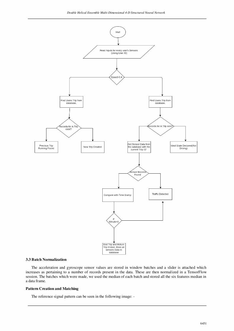
In Fig. 3 shows us the demonstration of different Gyro sensor information plotted in red , blue and yellow .

Here Z_median is denoted by yellow , Y_median by red and the data through port Gyro 110409 . The basic details

of the data are , the blue curve distribution is scaled in between 2 to -5 , it seeks low variance , kurtosis and also a

greater positive slope than negative currents on the curve. The Z directional median shows rough peaks and

troughs both are expectedly depicting a sinusoidal wave with pretty high variance , kurtosis and the slope is pretty

balanced over the region . Its min max range is from +7 to -14 . The Y directional median shows rough peaks and

troughs both are expectedly depicting a downward wave with pretty high negative variance , kurtosis and the

slope is pretty negative over the region . Its min max range is from +10 to -12 . The depiction also underlines the

usage of a certain Gyro sensor attached to a certain experimental vehicle working over for about 3000+

milliseconds.


6454

Figure.3.Demonstration of different Gyro sensor informationand Figure.4.Demonstration of different Gyro

sensor information

Fig. 4 shows us the demonstration of different Gyro sensor information plotted in red, blue and yellow. Here

Z_median is denoted by yellow, Y_median by red and the data through port Gyro 110343 id Y_gyro. As with

previous Fig. 2 understanding we can say that Y_gyro wave curve is quite persistent among it ranges of 5 and -5,

again the yellow curve shows a sinusoidal nature and downward drift to the red curve, here on we are seeing

similarity behavior to Fig. 3.

Figure.5. Demonstration of different Gyro sensor information and Figure.6. Demonstration of different Gyro

sensor information

In Fig. 5 shows us the demonstration of different Gyro sensor information plotted in red, blue and yellow.

Here Z_median is denoted by yellow, Y_median by red and the data through port Gyro 110321 id Y_gyro.

Y_gyro wave curve is pretty persistent among it ranges of 0 and -5, again the yellow curve shows non - sinusoidal

nature unlike the previous examples and downward drift to the red curve is pretty reluctant although with pretty

high troughs, this shows kind of abnormality about the behavior of driver 110321.In Fig. 6 shows us the

demonstration of different Gyro sensor information plotted in red, blue and yellow. Here Z_median is denoted by

yellow, Y_median by red and the data through port Gyro 110244 id Y_gyro. Y_gyro wave curve is pretty

persistent among it ranges of 0 and -5, again the yellow curve shows non - sinusoidal nature unlike the previous

examples and downward drift to the red curve is pretty reluctant although with pretty high troughs, this shows

kind of abnormality about the behavior of driver 110244 which matches our observation to Fig. 5.


Here Z_median is denoted by yellow, Y_median by red and the data through port Gyro 105503 id Y_gyro.

Y_gyro wave curve is pretty persistent among it ranges of 0 and -5 however it’s pretty normalized within this

scale , again the yellow curve shows non - sinusoidal nature unlike the previous examples and downward drift to

the red curve is pretty reluctant although with pretty high trough is seemed at the end of 3000th millisecond , this

shows kind of abnormality about the behavior of driver 105503 which matches our observation to Fig. 5 and 6.In

Fig. 8 Gyro sensor information plotted in red , blue and yellow .Here Z_median is denoted by yellow , Y_median

by red and the data through port Gyro 105503 id Y_gyro . This shows kind of abnormality about the behavior of

driver 105503 which matches our observation to Fig. 5 and 6. This graph traces for the 3000 second abnormality

of the driver.

Fig. 9 shows us the demonstration of different Gyro sensor information plotted in red, blue and yellow. Here

Z_median is denoted by yellow, Y_median by red and the data through port Gyro 105449 id Y_gyro. This shows

kind of abnormality about the behavior of driver 105449 which is especially unique because here, we do

mathematically observe a pattern which is a drifting sinusoidal wave, again the blue wave pretends to be pretty

normalized and red trough rise is still semantic to our previous observations. Henceforth, this is a sheerness of


6455

normal figure like Fig. 3 and 4, it is an interesting result in response to different graphical analysis earlier. Its

significance of this test results would be further classified in the conclusion section.In Fig. 10 shows us the

demonstration of different Gyro sensor information plotted in red, blue and yellow. Here Z_median is denoted by

yellow, Y_median by red and the data through port Gyro 105433 id Y_gyro. This shows kind of abnormality

about the behavior of driver 105433 which showcase high variance yellow sinusoidal wave, this instance the blue

wave pretends to be pretty variated in response to our previous normalized observation and red trough rise is still

semantic to our previous observations, however this rise is pretty steep and is above to both the curves with a

certain degree of superiority. Henceforth, this is again a sheerness of normalized plots such as Fig.3 and 4, but

differences from Fig. 11 do occur, it is an interesting result in response to different graphical analysis earlier. Its

significance of this test results would be further classified in the conclusion section.


sensor information


sensor information


Here Z_median is denoted by yellow, Y_median by red and the data through port Gyro 105402 id Y_gyro. This

shows kind of abnormality about the behavior of driver 105402 which showcase the presence of linearity or

readiness in authentic terms in all the three-dimensional wave curves, however when we twitch to our 2500

millisecond we see, the down growth of red stimulus and sinusoidal approach of yellow stimulus and pretty high

variance in the blue wave. These emerge as a partition boundary between two behavioral states of the driver’s

health or mental stimulus. These values of Gyroscope Y against the time for which they were recorded show a

large peak followed by a trough. This indication shows us that following an event, let’s say ‘x’ there is another

event which leads us to having noted that an event for correctional of ‘x’ happens almost immediately,

4.2. Classification Analysis

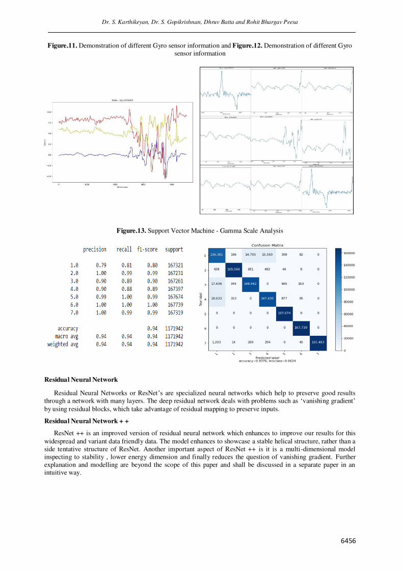
Support Vector Machine - Gamma Scale

A Support Vector Machine (SVM) is a discriminative classifier is defined by a separating hyperplane. In other

words, given labelled training data (supervised learning), the algorithm outputs an optimal hyperplane which

categorizes new examples. The gamma parameter defines how far the influence of a single training example

reaches, with low values meaning ‘far’ and high values meaning ‘close’. In other words, with low gamma, points

far away from plausible separation line are considered in the calculation for the separation line.


6456


sensor information

Figure.13. Support Vector Machine - Gamma Scale Analysis

Residual Neural Network

Residual Neural Networks or ResNet’s are specialized neural networks which help to preserve good results

through a network with many layers. The deep residual network deals with problems such as ‘vanishing gradient’

by using residual blocks, which take advantage of residual mapping to preserve inputs.

Residual Neural Network + +

ResNet ++ is an improved version of residual neural network which enhances to improve our results for this

widespread and variant data friendly data. The model enhances to showcase a stable helical structure, rather than a

side tentative structure of ResNet. Another important aspect of ResNet ++ is it is a multi-dimensional model

inspecting to stability , lower energy dimension and finally reduces the question of vanishing gradient. Further

explanation and modelling are beyond the scope of this paper and shall be discussed in a separate paper in an

intuitive way.


6457

Figure.14. Residual Neural Network Analysis

Figure.15. Residual Neural Network + + Analysis

5. Conclusion

This paper presents two-pronged way to approach driving behaviour.

Detection and Designation of events according to the activity pattern found via pattern matching

algorithm.

Classifying future events with the help of learning algorithms such as Support Vector Machines, ResNet

and ResNet++

Our system leverages inertial sensors integrated in smartphone and accomplish the objective of distinguishing

events of rash driving from normal driving without relying on any additional equipment. We evaluate each

process of detection, including activity recognition and show that our system achieves good specificity, accuracy

and precision, which leads to the high accuracy. Through evaluation, the accuracy of successful detection using

our own model ResNet++ which is modified and improved version of ResNet our accuracy is 94%, and the

precision is 96.67%. The evaluation of is based not only on the assumption that smartphone is attached to the user

body most of the time. Although, there were many such conditions which brought us a lot of difficulties, the

ResNet++ model still demonstrated to be robust in handling the detection through evidence fusion and some side

rough signals.With this, different drivers can be easily compared by means of the synthetic score. This synthetic score can be used to solve issues such as dealing with usage-based insurance, creation of a license score.


6458

References

Bergasa, L. M., Nuevo, J., Sotelo, M. A., Barea, R., & Lopez, M. E. (2006). Real-time system for monitoring

driver vigilance. IEEE Transactions on Intelligent Transportation Systems, 7(1), 63-77.

Bao, L., And Intille, S. Activity Recognition From User-Annotated Acceleration Data. Pervasive Computing

(2004), 1–17.

Chen, S. H., Pan, J. S., & Lu, K. (2015, March). Driving behavior analysis based on vehicle OBD information and

adaboost algorithms. In Proceedings of the international multiconference of engineers and computer scientists

(Vol. 1, pp. 18-20).

Chu, H. L., Raman, V., Shen, J., Choudhury, R. R., Kansal, A., And Bahl, V. Poster: You Driving? Talk To You

Later. In Mobisys (2011), Acm, Pp. 397–398.

Fugiglando, U., Santi, P., Milardo, S., Abida, K., &Ratti, C. (2017, October). Characterizing the" driver dna"

through can bus data analysis. In Proceedings of the 2nd ACM International Workshop on Smart,

Autonomous, and Connected Vehicular Systems and Services (pp. 37-41).

Hermannstädter, P., & Yang, B. (2013, October). Driver distraction assessment using driver modeling. In 2013

IEEE international conference on systems, man, and cybernetics (pp. 3693-3698). IEEE.

Kutila, M., Jokela, M., Markkula, G., And Rue, M. Driver Distraction Detection With A Camera Vision System.

In Icip (2007), Vol. 6, Ieee, Pp. Vi–201.

Lee, S., And Mase, K. Activity And Location Recognition Using Wearable Sensors. Pervasive Computing, Ieee 1,

3 (2002), 24–32.

Salvucci, D. Predicting The Effects Of In-Car Interfaces On Driver Behavior Using A Cognitive Architecture. In

Sigchi (2001), Acm, Pp. 120–127.

Singh, H., Bhatia, J. S., & Kaur, J. (2011, January). Eye tracking based driver fatigue monitoring and warning

system. In India International Conference on Power Electronics 2010 (IICPE2010) (pp. 1-6). IEEE.

Youssef, M., Yosef, M., And El-Derini, M. Gac: Energy-Efficient Hybrid Gps-Accelerometer-Compass Gsm

Localization. In Globecom (2010), IEEE, Pp. 1–5.

double helical ensemble multi-dimensional 4-d structured

Documents