dot/faa/ar-00/14 effects of large-droplet ice accretion on

DOT/FAA/AR-00/14

Office of Aviation ResearchWashington, D.C. 20591

Effects of Large-Droplet IceAccretion on Airfoil andWing Aerodynamics andControl

March 2000

Final Report

This document is available to the U.S. publicthrough the National Technical InformationService (NTIS), Springfield, Virginia 22161.

U.S. Department of TransportationFederal Aviation Administration

NOTICE

This document is disseminated under the sponsorship of the U.S.Department of Transportation in the interest of information exchange. TheUnited States Government assumes no liability for the contents or usethereof. The United States Government does not endorse products ormanufacturers. Trade or manufacturer's names appear herein solely becausethey are considered essential to the objective of this report. This documentdoes not constitute FAA certification policy. Consult your local FAA aircraftcertification office as to its use.

This report is available at the Federal Aviation Administration William J.Hughes Technical Center’s Full-Text Technical Reports page:www.actlibrary.tc.faa.gov in Adobe Acrobat portable document form (PDF).

Technical Report Documentation Page1. Report No.

DOT/FAA/AR-00/14

2. Government Accession No. 3. Recipient's Catalog No.

4. Title and Subtitle

EFFECTS OF LARGE-DROPLET ICE ACCREATION ON AIRFOIL AND WING

5. Report Date

March 2000AERODYNAMICS AND CONTROL 6. Performing Organization Code

7. Author(s)

Michael B. Bragg and Eric Loth

8. Performing Organization Report No.

9. Performing Organization Name and Address

University of Illinois at Urbana-Champaign

10. Work Unit No. (TRAIS)

Aeronautical and Astronautical EngineeringUrbana, IL 61801

11. Contract or Grant No.

12. Sponsoring Agency Name and Address

U.S. Department of TransportationFederal Aviation Administration

13. Type of Report and Period Covered

Final Report

Office of Aviation ResearchWashington, DC 20591

14. Sponsoring Agency Code

AIR-10015. Supplementary Notes

The Federal Aviation Administration William J. Hughes Technical Center technical manager was James Riley.16. Abstract

An integrated experimental and computational investigation was conducted to determine the effect of simulated ridge ice shapeson airfoil aerodynamics. These upper-surface shapes are representative of those which may form aft of protected surfaces insuper-cooled large droplet conditions. The simulated ice shapes were experimentally tested on a modified NACA 23012(23012m) airfoil and NLF 0414 airfoil at Reynolds numbers of 1.8 million for a range of protuberance locations, sizes, andshapes. The computational study investigated the cases encompassed by the experimental study but in addition includedhigher Reynolds numbers and other airfoils from the NASA Commuter Airfoil Program.

The simulated ice shapes produced very different results on the NACA 23012m and the NLF airfoils, which was primarilyattributed to their very different pressure distributions without ice. The effects of the simulated ice shapes were much moresevere on the forward-loaded NACA 23012m, with a measured Cl, max as low as 0.25 from the ice shape with a height-to-chord

ratio of 0.0139 and an x/c of .12. The lowest true Cl, max measured for the NLF 0414 with the same ice shape was 0.68.

Various simulated ice shape sizes and geometries were also investigated on both airfoils. Aerodynamic penalties became moresever as the height-to-chord ratio of the simulated ice shape was increased from .0056 to .0139. The variation in the simulatedice shape geometry had only minor effects on the airfoil aerodynamics.

The numerical investigation included steady-state simulations with a high-resolution full Navier-Stokes solver using asolution-adaptive unstructured grid for both non-iced and iced configurations. The effect of ice shape size, geometry, location,Reynolds number, flap deflection and airfoil geometry was reasonably reproduced by computational methodology for a widerange of the experimental conditions. The airfoil shape sensitivity studies indicated that the NACA 23012m exhibited themost detrimental performance with respect to lift loss, which tended to be greatest around x/c of about 0.1 which alsocorresponds to the location of minimum pressure coefficient (Cp.). However, the more evenly loaded NLF 0414 tended to haveless separation for equivalent clean airfoil lift conditions and did not exhibit a unique critical ice shape location. Both theGLC 305 and the Boeing 747/767 horizontal tailplane airfoils had very high suction peaks near the leading edge (x/c = 0.02),closest to the location of its minimum Cp. Finally, Reynolds number effects for the iced airfoil cases were found to benegligible (unlike that for the clean airfoil cases.)

17. Key Words

Super-cooled large droplets, Ridge ice accretion, Airfoil,Aerodynamic penalty

18. Distribution Statement

This document is available to the public through the NationalTechnical Information Service (NTIS), Springfield, Virginia22161.

19. Security Classif. (of this report)

Unclassified20. Security Classif. (of this page)

Unclassified21. No. of Pages

19522. Price

Form DOT F1700.7 (8-72) Reproduction of completed page authorized

iii

TABLE OF CONTENTS

Page

EXECUTIVE SUMMARY xix

1. INTRODUCTION 1

1.1 Review of Literature–Experimental 21.2 Review of Literature–Computational 3

1.2.1 Leading-Edge Ice Shapes 31.2.2 Upper-Surface Ridge Ice Shapes 5

1.3 Research Objectives 61.4 Research Overiew 6

2. RESEARCH METHODOLOGY 7

2.1 Experimental Methodology 7

2.1.1 Wind Tunnel 72.1.2 Airfoil Models 92.1.3 Force and Moment Balance 92.1.4 Flap Actuator and Balance 112.1.5 Wake Survey System 112.1.6 Digital Pressure Acquisition System 122.1.7 Ice Simulation 132.1.8 Data Acquisition and Reduction 14

2.2 Computational Methodology 16

2.2.1 Flow Solution 17

2.2.1.1 Governing Equations 172.2.1.2 Spatial Discretization 192.2.1.3 Time Discretization 212.2.1.4 Convergence Acceleration Techniques 232.2.1.5 Turbulence Model 24

2.2.2 Grid Generation 27

2.2.2.1 Commonly Used Grid Generation Techniques 282.2.2.2 Grid Generation Techniques Used in UMESH2D 29

2.2.3 Grid Adaptivity, Refinement, and Interpolation 31

iv

2.2.4 Postprocessing and Data Reduction 33

3. VALIDATION 34

3.1 NACA 23012 Coordinate Modification 343.2 Experimental Validation 383.3 Code Validation 40

3.3.1 Simple Geometry Flow Field Simulation 41

3.3.1.1 Flat-Plate Boundary Layer 413.3.1.2 Laminar Boundary Layer 423.3.1.3 Turbulent Boundary Layer 423.3.1.4 Backward-Facing Step 43

3.3.2 Clean Airfoil Simulations 45

3.3.2.1 NACA 0012 453.3.2.2 NACA 23012 503.3.2.3 NACA 23012m With an Undeflected Flap 513.3.2.4 NACA 23012m With Tunnel Walls 573.3.2.5 NLF 0414 Simulations 60

3.3.3 Iced Airfoil SimulationsNACA 0012 With Glaze Ice 63

3.4 Airfoil Stall Types 68

4. RESULTS AND DISCUSSION 69

4.1 Experimental Results 69

4.1.1 Effect of Simulated Ice Ridge Location 70

4.1.1.1 Effects of Flap Deflection 744.1.1.2 Flow Field Analysis 774.1.1.3 Pitching and Flap Hinge Moment Analysis 81

4.1.2 Effects of Simulated Ice Shape Size 824.1.3 Effect of Simulated Ice Shape Geometry 854.1.4 Effects of Roughness Near Ice Shape 874.1.5 Effects of Spanwise Gaps 894.1.6 Effect of Simulated Ice Accretion on the Lower Surface 914.1.7 Effects of Airfoil Geometry 93

4.1.7.1 Comparison of Clean Models 934.1.7.2 Effect of Ice shape Locations 94

v

4.1.7.3 Flow Field Comparisons 101

4.2 COMPUTATIONAL RESULTS 103

4.2.1 NACA 23012m Iced Airfoil Results 103

4.2.1.1 Computational Prediction Fidelity for Icing 1034.2.1.2 Effects of Variation in Size 1104.2.1.3 Effects of Variation in Ice Shape Location 1154.2.1.4 Effects of Variation in Ice Shape Geometry 1224.2.1.5 Effects of Flap Deflection 1254.2.1.6 Effects of Variation in Reynolds Number 129

4.2.2 Other Iced Airfoil Simulations 132

4.2.2.1 NLF Airfoil Results 1344.2.2.2 Business Jet Model Airfoil Results 1434.2.2.3 Large Transport Horizontal Stabilizer Airfoil Results 1484.2.2.4 Comparative Study of the Four Airfoils 151

4.3 Experimental Data CD-ROM 160

5. CONCLUSIONS 166

5.1 Primary Conclusions 1665.2 Experimental Study Conclusions 1675.3 Computational Study Conclusions 169

6. REFERENCES 171

vi

LIST OF FIGURES

Figure Page

1 Large Droplet Ice Accretion on a NACA 23012 Airfoil in the NASA Glenn IcingResearch Tunnel 1

2 Schematic of the Experimental Setup 8

3 University of Illinois 3′ × 4′ Subsonic Wind Tunnel 8

4 Surface Pressure Tap Locations for the NACA 23012m and NLF 0414 AirfoilModels 10

5 Three-Component Force Balance 11

6 Wake Rake 12

7 Ice Shape Simulation Geometry 13

8 NACA 23012 Model With Quarter-Round Ice Simulation 14

9 Flowchart of the Overall Computational Strategy 17

10 Mesh Generation Stages, (a) Geometry, (b) Spline and Wake, (c) Viscous Grid(Far Field), (d) Viscous Grid (Closeup), (e) Final Grid (Far Field), and (f) FinalGrid (Closeup) 28

11 Original Grid Near Quarter-Round Shape. 31

12 Adapted Grid Near Quarter-Round Shape 32

13 Absolute Velocity Contours for Original Grid 33

14 Geometry Comparison Between Modified NACA 23012m Used in this Studyand Standard NACA 23012 36

15 Lift Comparison Between Modified NACA 23012m Used in this Study andStandard NACA 23012, Results From XFOIL, Re = 1.8 × 106 37

16 Surface Pressure Comparison Between Modified NACA 23012m Used in thisStudy and Standard NACA 23012, Results From XFOIL, Re = 1.8 × 106 37

17 Aerodynamic Coefficients of the Clean NACA 23012m Airfoil 39

18 Surface Pressure of the Clean NACA 23012m Airfoil. 40

19 Streamwise Velocity in Laminar Boundary Layer in Terms of SimilarityCoordinates 41

vii

20 Streamwise Velocity Profile in Turbulent Boundary Layer in Terms of PhysicalCoordinates 42

21 Reattachment Length Past A Backward-Facing Step 44

22 Mean Velocity Profiles Past A Backward-Facing Step 45

23 Effect of Variation in Reynolds Number on Lift for a NACA 0012 Airfoil atMach Number 0.15 46

24 Effect of Variation in Reynolds Number on Drag for a NACA 0012 Airfoil atMach Number 0.15 47

25 Effect of Variation in Reynolds Number on Pitching Moment for a NACA 0012Airfoil at Mach Number 0.15 47

26 Effect of Variation in Mach Number on Lift for a NACA 0012 Airfoil at ReynoldsNumber 6 Million 48

27 Effect of Variation in Mach Number on Drag for a NACA 0012 Airfoil at ReynoldsNumber 6 Million 49

28 Effect of Variation in Mach Number on Pitching Moment for a NACA 0012Airfoil at Reynolds Number 6 Million 49

29 Lift Coefficients for a NACA 23012 Airfoil 50

30 Drag Coefficients for a NACA 23012 Airfoil 51

31 Mesh for NACA 23012m, (a) Far Field, (b) Closeup, and (c) Flap 52

32 Lift Coefficients for a NACA 23012m Airfoil 54

33 Drag Coefficients for a NACA 23012m Airfoil 54

34 Pictching Moment Coefficients for a NACA 23012m Airfoil 55

35 Hinge Moment Coefficients for a NACA 23012m Airfoil 55

36 Surface Pressure Distribution for a NACA 23012m Airfoil at α = 4.1447° 56

37 Surface Pressure Distribution for a NACA 23012m Airfoil at α = 12.358° 56

38 Mesh for NACA 23012m in Tunnel at α = 10.0°, (a) Outer Boundary Region,(b) Far Field, and (c) Closeup 57

39 Lift Coefficients for a NACA 23012m Airfoil Modeled for Two Methods(1) Euler-Walls Where the Tunnel Walls (and Corrected Using the Theory of Raeand Pope) and (2) Far Field Where the Airfoil Was Simulated Without Tunnel Walls 58

viii

40 Drag Coefficients for a NACA 23012m Airfoil Modeled With Tunnel Walls WereSimulated Directly and Subsequently Corrected Using the Theory of Rae and Popeto Free Flight Conditions and Far Field Where the Airfoil Was Simulated WithoutTunnel Walls 59

41 Pitching Moment Coefficients for a NACA 23012m Airfoil Modeled With TunnelWalls (and Corrected Using the Theory of Rae and Pope) and Without Tunnel Walls 59

42 Hinge Moment Coefficients for a NACA 23012m Airfoil Modeled With TunnelWalls (and Corrected Using the Theory of Rae and Pope) and Without Tunnel Walls 60

43 Lift Coefficients for a NLF 0414 Airfoil Modeled With Tunnel Walls 61

44 Drag Coefficients for a NLF 0414 Airfoil Modeled With Tunnel Walls 61

45 Pitching Moment Coefficients for a NLF 0414 Airfoil Modeled With Tunnel Walls 62

46 Hinge Moment Coefficients for a NLF 0414 Airfoil Modeled With Tunnel Walls 62

47 Surface Pressure Distribution for a NLF 0414 Airfoil at (a) α = -6°, (b) α = 0°,and (c) α = 10° 64

48 Mesh for NACA 0012m (a) Far Field Where Airfoil Is Inside the Clustered Grids,(b) Closeup of Airfoil, and (c) Closeup of Ice Shape 65

49 Lift Coefficients for a NACA 0012m Airfoil With Leading-Edge Glaze Ice 66

50 Drag Coefficients for a NACA 0012m Airfoil With Leading-Edge Glaze Ice 66

51 Moment Coefficients for a NACA 0012m Airfoil With Leading-Edge Glaze Ice 67

52 Surface Pressure Distribution for a NACA 0012m Airfoil With Leading-EdgeGlaze Ice at α = 4.12° 68

53 Lift Characteristics of the Three Airfoil Stall Types 69

54 Effects of Simulated Ice Shape Location on Aerodynamic Coefficients 71

55 Summary of Cl,max With Simulated Ice Shape at Various Locations 72

56 Drag Increase Due to Simulated Ice Shape at Various Locations 73

57 Lift Loss Due to Simulated Ice Shape at Various Locations 74

58 Effects of Flap Deflection on Aerodynamic Coefficients 75

59 Effects of Simulated Ice Shape on Flap Effectiveness 76

ix

60 Summary of Boundary Layer State With the Simulated Ice at x/c = 0.10 77

61 Reattachment Location of Separation Bubble That Formed Downstream ofSimulated Ice 78

62 Effect of Ice Shape Location on Surface Pressure Distribution 80

63 Effects of Simulated Ice Shape Size on Aerodynamic Coefficients 83

64 Effects of Simulated Ice Shape Size on Surface Pressures 84

65 Summary of Cl,max With Various Simulated Ice Shape Size and Locations 85

66 Effects of Simulated Ice Shape Geometry on Aerodynamic Coefficients 86

67 Effects of Surface Roughness in Addition to Simulated Ice Shape on AerodynamicCoefficients 88

68 Spanwise Gap Geometry 89

69 Effects of Spanwise Gap on Aerodynamic Coefficients 90

70 Effects of Lower Surface Simulated Ice Accretion on Aerodynamic Coefficients 92

71 Comparison of NACA 23012m and NLF 0414 Geometry 93

72 Comparison of NACA 23012m and NLF 0414 Clean Model Pressure Distribution 94

73 Effect of Simulated Ice Shape Location on Lift 95

74 Summary of Cl,max With 0.25″ Forward-Facing Quarter Round Simulated Ice

Shape at Various Chordwise Locations 96

75 Effect of Simulated Ice Shape Location on Drag 96

76 Effect of Simulated Ice Shape Location on Pitching Moment 97

77 Effect of Simulated Ice Shape Location on Flap Hinge Moment 98

78 Drag Increase Due to Ice Shape 99

79 Lift Loss Due to Ice Shape 100

80 Effect of Simulated Ice Shape Location on Surface Pressure 102

81 Lift Coefficients for a NACA 23012m With k/c = 0.0083 Quarter-Round IceShape Located at x/c = 0.1 104

x

82 Drag Coefficients for a NACA 23012m With k/c = 0.0083 Quarter-Round IceShape Located at x/c = 0.1 105

83 Pitching Moment Coefficients for a NACA 23012m With k/c = 0.0083 Quarter-Round Ice Shape Located at x/c = 0.1. 105

84 Hinge Moment Coefficients for a NACA 23012m With k/c = 0.0083 Quarter-Round Ice Shape Located at x/c = 0.1 106

85 Velocity Vectors at Sample Locations for a NACA 23012m With k/c = 0.0083Quarter-Round Ice Shape Located at x/c = 0.1 and α = -6° 106

86 Reattachment Locations of the Aft Ice Separation Bubble for a NACA 23012mWith k/c = 0.0083 Quarter-Round Ice Shape Located at x/c = 0.1 107

87 (a) Streamlines and (b) Surface Pressure Distributions For a NACA 23012m,With k/c = 0.0083 Quarter-Round Ice Shape Located at x/c = 0.1 and α = -6 108

88 (a) Streamlines and (b) Surface Pressure Distributions for a NACA 23012m,With k/c = 0.0083 Quarter-Round Ice Shape Located at x/c = 0.1 and α = 6° 109

89 Geometry of NACA 23012m With an Ice Shape Located at x/c = 0.1 With Heights(a) k/c = 0.0, (b) k/c = 0.0083, and (c) k/c = 0.0139 111

90 Effect of Shape Height on Lift for an Ice Shape Located at x/c = 0.1 112

91 Effect of Shape Height on Drag for an Ice Shape Located at x/c = 0.1 112

92 Effect of Shape Height on Pitching Moment for an Ice Shape Located at x/c = 0.1 113

93 Effect of Shape Height on Hinge Moment for an Ice Shape Located at x/c = 0.1 114

94 Effect of Shape Height on Pressure Distribution at α = 3° for an Ice ShapeLocated at x/c = 0.1 for Heights (a) k/c = 0.0, (b) k/c = 0.0083, and (c) k/c = 0.0139 115

95 Geometry of NACA 23012m With k/c = 0.0083 Ice Shape Located at (a) x/c = 0.1,(b) x/c = 0.2, and (c) x/c = 0.3 116

96 Effect of Shape Location on Lift for k/c = 0.0083 Ice Shape 117

97 Effect of Shape Location on Drag for k/c = 0.0083 Ice Shape 117

98 Effect of Shape Location on Pitching Moment for k/c = 0.0083 Ice Shape 118

99 Effect of Shape Location on Hinge Moment for k/c = 0.0083 Ice Shape 118

100 Effect of Shape Location on Pressure Distribution at α = 3° for k/c = 0.0083 IceShape Located at (a) x/c =0.1, (b) x/c = 0.2, and (c) x/c = 0.3 119

xi




104 Lift Coefficient for Angle of Attack at Which Flow First Fully Separates Vs.x/c for A NACA 23012m Airfoil With k/c = 0.0083 Quarter-Round Ice Shape 122

105 Effect of Ice Shape Geometry on Lift for k/c = 0.0139 Ice Shapes Located atx/c = 0.1 123

106 Effect of Ice Shape Geometry on Drag for k/c = 0.0139 Ice Shapes Located atx/c = 0.1 123

107 Effect of Ice Shape Geometry on Pitching Moment for k/c = 0.0139 Ice ShapesLocated at x/c = 0.1 124

108 Effect of Ice Shape Geometry on Hinge Moment for k/c = 0.0139 Ice ShapesLocated at x/c = 0.1 124

109 Effect of Flap Deflection on Lift for k/c = 0.0 125

110 Effect of Flap Deflection on Drag for k/c = 0.0 126

111 Effect of Flap Deflection on Pitching Moment for k/c = 0.0 126

112 Effect of Flap Deflection on Hinge Moment for k/c = 0.0 127

113 Effect of Flap Deflection on Lift for Iced Case With k/c = 0.0083 Located atx/c = 0.1 127

114 Effect of Flap Deflection on Drag for Iced Case With k/c = 0.0083 Located atx/c = 0.1 128

115 Effect of Flap Deflection on Pitching Moment for Iced Case With k/c = 0.0083Located at x/c = 0.1 128

116 Effect of Flap Deflection on Hinge Moment for Iced Case With k/c = 0.0083Located at x/c = 0.1 129

117 Effect of Reynolds Number on Lift for k/c = 0.0083 Ice Shape Locatedat x/c = 0.1 130

118 Effect of Reynolds Number on Drag for k/c = 0.0083 Ice Shape Locatedat x/c = 0.1 130

xii

119 Effect of Reynolds Number on Pitching Moment for k/c = 0.0083 Ice ShapeLocated at x/c = 0.1 131

120 Effect of Reynolds Number on Hinge Moment for k/c = 0.0083 Ice ShapeLocated at x/c = 0.1 131

121 Surface Pressure Distribution for a Clean NACA 23012m Airfoil for anEquivalent C l = 0.5 at α = 4° 132

122 Surface Pressure Distribution for a Clean NLF 0414 Airfoil for an EquivalentC l = 0.5 at α = 0° 133

123 Surface Pressure Distribution for a Clean Business Jet Model Airfoil for anEquivalent C l = 0.5 at α = 4° 133

124 Surface Pressure Distribution for a Clean Large Transport Horizontal StabilizerAirfoil for an Equivalent C l = 0.5 at α = 4° 134

125 Effect of Ice Shape Location on Lift for k/c = 0.0083 Ice Shapes for theNLF Airfoil 135

126 Effect of Ice Shape Location on Drag for k/c = 0.0083 Ice Shapes for theNLF Airfoil 135

127 Effect of Ice Shape Location on Pitching Moment for k/c = 0.0083 Ice Shapesfor the NLF Airfoil 136

128 Effect of Ice Shape Location on Hinge Moment for k/c = 0.0083 Ice Shapes forthe NLF Airfoil 136

129 Reattachment Locations of the Aft Ice Separation Bubble for a NLF 0414 AirfoilWith k/c = 0.0083 Quarter-Round Ice Shape Located at x/c = 0.02 137



132 Lift Coefficient for Angle of Attack at Which Flow First Fully Separates Vs. x/cfor a NLF 0414 With k/c = 0.0083 Quarter-Round Ice Shape 139

133 Effect of Ice Shape on Lift for a NLF 0414 Airfoil With Quarter-Round Ice ShapeLocated at x/c = 0.1 140

134 Effect of Ice Shape Height on Drag for a NLF 0414 Airfoil With a Quarter-RoundIce Shape Located at x/c = 0.1 141

xiii

135 Effect of Ice Shape Height on Pitching Moment for a NLF Airfoil WithQuarter-Round Ice Shape Located at x/c = 0.1 142

136 Effect of Ice Shape Height on Hinge Moment for a NLF 0414 Airfoil With aQuarter-Round Ice Shape Located at x/c = 0.1 143

137 Effect of Ice Shape Location on Lift for k/c = 0.0083 Ice Shapes for theBusiness Jet Model Airfoil 144

138 Effect of Ice Shape Location on Drag for k/c = 0.0083 Ice Shapes for theBusiness Jet Model Airfoil 144

139 Effect of Ice Shape Location on Pitching Moment for k/c = 0.0083 Ice Shapes forthe Business Jet Model Airfoil 145

140 Effect of Ice Shape Location on Hinge Moment for k/c = 0.0083 Ice Shapes forthe Business Jet Model Airfoil 145

141 Reattachment Locations of the Aft Ice Separation Bubble for a Business Jet ModelAirfoil With k/c = 0.0083 Quarter-Round Ice Shape Located at x/c = 0.02 146



144 Lift Coeeficient for Angle of Attack at Which Flow First Fully Separates Vs. x/cfor a Business Jet Model With k/c = 0.0083 Quarter-Round Ice Shape 148

145 Effect of Ice Shape Location on Lift for k/c = 0.0083 Ice Shapes for theLarge Transport Horizontal Stabilizer 149

146 Effect of Ice Shape Location on Drag for k/c = 0.0083 Ice Shapes for the LargeTransport Horizontal Stabilizer 150

147 Effect of Ice Shape Location on Pitching Moment for k/c = 0.0083 Ice Shapes forthe Large Transport Horizontal Stabilizer 150

148 Effect of Ice Shape Location on Hinge Moment for k/c = 0.0083 Ice Shapes for theLarge Transport Horizontal Stabilizer 151

149 Comparison of Airfoil Geometries With k/c = 0.0083 Ice Shape Located atx/c = 0.1 152

150 Effect of Airfoil Geometry on Lift for k/c = 0.0083 Ice Shape Located atx/c = 0.1 153

xiv

151 Effect of Airfoil Geometry on Drag for k/c = 0.0083 Ice Shape Located atx/c = 0.1 153

152 Effect of Airfoil Geometry on Pitching Moment for k/c = 0.0083 Ice ShapeLocated at x/c = 0.1 154

153 Effect of Airfoil Geometry on Hinge Moment for k/c = 0.0083 Ice ShapeLocated at x/c = 0.1 154

154 Streamlines and Surface Pressure Distributions for a NACA 23012m AirfoilWith k/c = 0.0083 Quarter-Round Ice Shape Located at x/c = 0.1 and α = 3° 156

155 Streamlines and Surface Pressure Distributions for a NLF 0414 Airfoil Withk/c = 0.0083 Quarter-Round Ice Shape Located at x/c = 0.1 and α = -2° 157

156 Streamlines and Surface Pressure Distributions for a Business Jet Model AirfoilWith k/c = 0.0083 Quarter-Round Ice Shape Located at x/c = 0.1 and α = 2° 158

157 Streamlines and Surface Pressure Distributions for Large Transport HorizontalStabilizer Airfoil With k/c = 0.0083 Quarter-Round Ice Shape Located at x/c = 0.1and α = 3° 159

xv

LIST OF TABLES

Table Page

1 Experimental Uncertainties for the Clean NACA 23012m Model at α = 5º,Re = 1.8 Million 15

2 Standard NACA 23012 and Modified NACA 23012m Coordinates 35

3 Format of Integrated Aerodynamic Coefficient Data Files 161

4 Format of the Surface Pressure Coefficient Data Files 161

5 No Simulated Ice Airfoil Data 161

6 Forward-Facing Quarter Round, k = 0.25″, NACA 23012m 162



9 Various Simulated Ice Shape Geometry, k = 0.25″, Re = 1.8 × 106, NACA 23012m 164

10 Forward-Facing Quarter Round on Upper and Lower Surface of the Model atx/c = 0.10, k = 0.25″, Re = 1.8 × 106, NACA 23012m 164

11 Spanwise Gaps in the Simulated Ice Shapes, Forward-Facing Quarter Round,k = 0.25″, Re = 1.8 × 106, NACA 23012m 165

12 Roughness Upstream and Downstream of Simulated Ice Shape, Forward-FacingQuarter Round, k = 0.25″, Re = 1.8 × 106, NACA 23012m 165

13 16-Grit Roughness, 0.25″ Chordwise Extent, Re = 1.8 × 106, NACA 23012m 165

14 Forward-Facing Quarter Round, k = 0.25″, NLF 0414 166

xvi

LIST OF ABBREVIATIONS AND SYMBOLS

LETTERSA Area of the elementCd Drag coefficient, D’/(q∞c)Cf Skin friction coefficientCh Flap hinge moment coefficient, H’/(q∞cf

2)Ch,α Flap hinge moment curve slopeCl Lift coefficient, L’/(q∞c)Cl,max Maximum lift coefficientCl,α Lift curve slopeCl,δf Change in lift with flap deflectionCm Pitching moment coefficient, M’/(q∞c2)Cm,α Pitching moment curve slopeCm,δf Change in pitching moment with flap deflectionCn Normal force coefficient, N’/(q∞c)Cp Pressure coefficient, (p-p∞)/q∞CFL Inviscid Courant NumberD’ Drag per unit spanE’ Fluid total energyFc Convective fluxFv Viscous fluxH Step heightH’ Flap hinge moment per unit spanLWC Liquid water contentL’ Lift per unit spanLAB Length of edge ABM Mach numberMVD Mean volumetric diameterM’ Pitching moment per unit spanN Normal force per unit spanNi Linear shape function of node IPr Prandtl numberPrt Turbulent Prandtl numberRe Chord-based Reynolds number, (ρV∞c)/µT Fluid temperatureV∞ Freestream velocitya Speed of soundc Airfoil chordcf Flap chordfc,gc Cartesian components of convective fluxfv,gv Cartesian components of viscous fluxk Protuberance heightn)

Unit normal vectorp Fluid static pressurep0 Total pressure in the wakep∞,0 Freestream total pressurep∞ Freestream static pressureq Heat flux vectorqw Dynamic pressure in the wakeq∞ Freestream dynamic pressureu.v Cartesian components of the velocity vectorue Edge velocity

xvii/xviii

u+ Law of the wall inner variable, u/v*

v* Wall friction velocity, (τw/ρ)1/2

w Solution vector of the conservative variablesx Airfoil coordinate in chordwise directionxR Reattachment lengthxr Reattachment locationy Airfoil coordinate perpendicular to chordy+ Law of the wall inner variable, (yv*)/νz Airfoil coordinate in spanwise direction

SYMBOLS∆Cd Drag increase due to ice accretion, Cd – Cd,clean∆Cl Lift loss due to ice accretion, Cl,clean – Cl∆t Local time stepΩ Area of the domainα Angle of attackδ Top wall deflection angleδf Flap deflectionφ Galerkin test functionγ Specific heat ratioε Blasius similarity variableµ Molecular viscosityµt Eddy viscosityν Kinematic viscosityν~ Spalart-Allmaras working variableνt Turbulent kinematic viscosityρ Fluid densityσ Stress tensorτw Wall shear stress, µ(du/dy)w

SUBSCRIPTSx,y Components in x,y directions∞ Freestream value

SUPERSCRIPTS^ Dimensional variable

xix/xx

EXECUTIVE SUMMARY

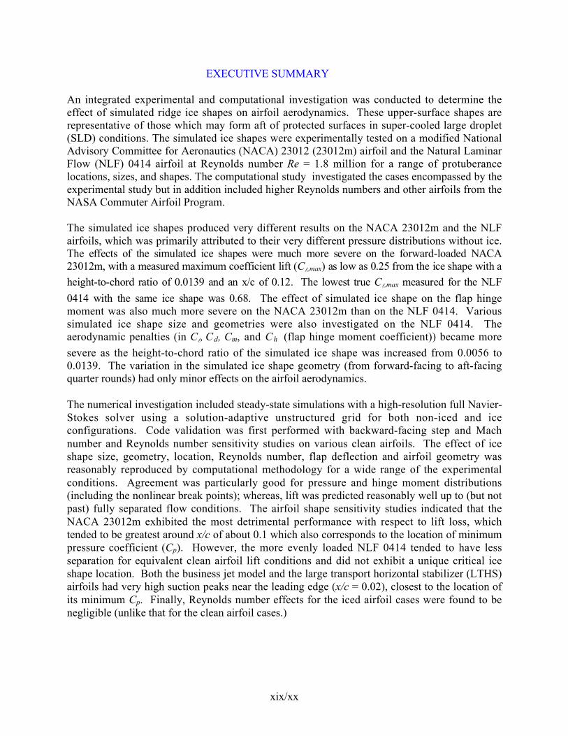
An integrated experimental and computational investigation was conducted to determine theeffect of simulated ridge ice shapes on airfoil aerodynamics. These upper-surface shapes arerepresentative of those which may form aft of protected surfaces in super-cooled large droplet(SLD) conditions. The simulated ice shapes were experimentally tested on a modified NationalAdvisory Committee for Aeronautics (NACA) 23012 (23012m) airfoil and the Natural LaminarFlow (NLF) 0414 airfoil at Reynolds number Re = 1.8 million for a range of protuberancelocations, sizes, and shapes. The computational study investigated the cases encompassed by theexperimental study but in addition included higher Reynolds numbers and other airfoils from theNASA Commuter Airfoil Program.

The simulated ice shapes produced very different results on the NACA 23012m and the NLFairfoils, which was primarily attributed to their very different pressure distributions without ice.The eff ect s of the simulat ed ice shapes were much more sever e on the forward-loaded NACA23012m, wi th a measured maxi mum coef ficient lif t ( Cl,max) as low as 0.25 f rom t he ice shape wit h a

height- to- chord rati o of 0.0139 and an x/c of 0.12. The lowest tr ue Cl,max measur ed for the NL F

0414 wi th the same ice shape was 0.68. The effect of simulated ice shape on the flap hingemoment was also much more severe on the NACA 23012m than on the NLF 0414. Varioussimulated ice shape size and geometries were also investigated on the NLF 0414. Theaerodynamic penalties (in Cl, Cd, Cm, and Ch (flap hinge moment coefficient)) became more

severe as the height-to-chord ratio of the simulated ice shape was increased from 0.0056 to0.0139. The variation in the simulated ice shape geometry (from forward-facing to aft-facingquarter rounds) had only minor effects on the airfoil aerodynamics.

The numerical investigation included steady-state simulations with a high-resolution full Navier-Stokes solver using a solution-adaptive unstructured grid for both non-iced and iceconfigurations. Code validation was first performed with backward-facing step and Machnumber and Reynolds number sensitivity studies on various clean airfoils. The effect of iceshape size, geometry, location, Reynolds number, flap deflection and airfoil geometry wasreasonably reproduced by computational methodology for a wide range of the experimentalconditions. Agreement was particularly good for pressure and hinge moment distributions(including the nonlinear break points); whereas, lift was predicted reasonably well up to (but notpast) fully separated flow conditions. The airfoil shape sensitivity studies indicated that theNACA 23012m exhibited the most detrimental performance with respect to lift loss, whichtended to be greatest around x/c of about 0.1 which also corresponds to the location of minimumpressure coefficient (Cp). However, the more evenly loaded NLF 0414 tended to have lessseparation for equivalent clean airfoil lift conditions and did not exhibit a unique critical iceshape location. Both the business jet model and the large transport horizontal stabilizer (LTHS)airfoils had very high suction peaks near the leading edge (x/c = 0.02), closest to the location ofits minimum Cp. Finally, Reynolds number effects for the iced airfoil cases were found to benegligible (unlike that for the clean airfoil cases.)

1

1. INTRODUCTION.

Aircraft can accrete ice on its aerodynamic surfaces when flying through clouds of super-cooledwater droplets. The size and shape of the ice accretion on unprotected aerodynamic surfacesdepend primarily on airspeed, temperature, water droplet size, liquid water content, and theperiod of time the aircraft has operated in the icing condition.

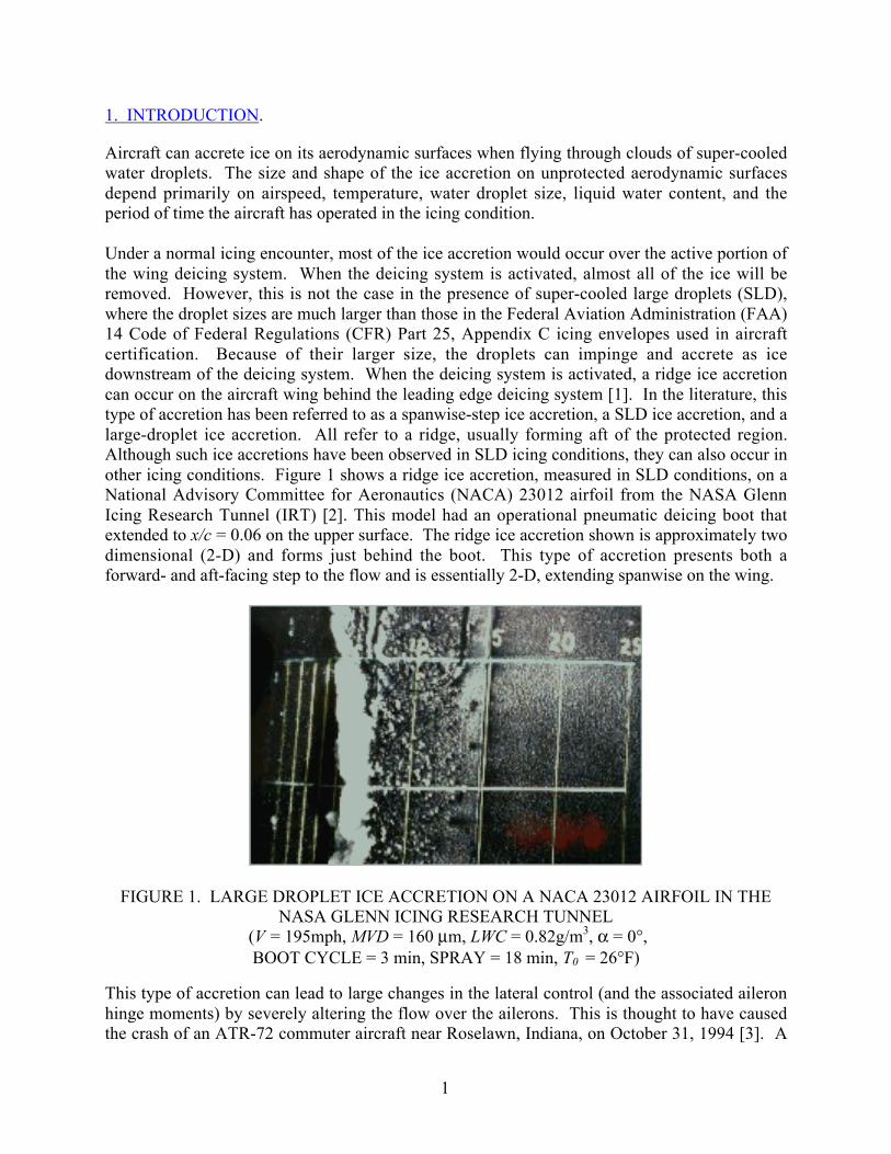
Under a normal icing encounter, most of the ice accretion would occur over the active portion ofthe wing deicing system. When the deicing system is activated, almost all of the ice will beremoved. However, this is not the case in the presence of super-cooled large droplets (SLD),where the droplet sizes are much larger than those in the Federal Aviation Administration (FAA)14 Code of Federal Regulations (CFR) Part 25, Appendix C icing envelopes used in aircraftcertification. Because of their larger size, the droplets can impinge and accrete as icedownstream of the deicing system. When the deicing system is activated, a ridge ice accretioncan occur on the aircraft wing behind the leading edge deicing system [1]. In the literature, thistype of accretion has been referred to as a spanwise-step ice accretion, a SLD ice accretion, and alarge-droplet ice accretion. All refer to a ridge, usually forming aft of the protected region.Although such ice accretions have been observed in SLD icing conditions, they can also occur inother icing conditions. Figure 1 shows a ridge ice accretion, measured in SLD conditions, on aNational Advisory Committee for Aeronautics (NACA) 23012 airfoil from the NASA GlennIcing Research Tunnel (IRT) [2]. This model had an operational pneumatic deicing boot thatextended to x/c = 0.06 on the upper surface. The ridge ice accretion shown is approximately twodimensional (2-D) and forms just behind the boot. This type of accretion presents both aforward- and aft-facing step to the flow and is essentially 2-D, extending spanwise on the wing.

FIGURE 1. LARGE DROPLET ICE ACCRETION ON A NACA 23012 AIRFOIL IN THENASA GLENN ICING RESEARCH TUNNEL

(V = 195mph, MVD = 160 µm, LWC = 0.82g/m3, α = 0°,BOOT CYCLE = 3 min, SPRAY = 18 min, T0 = 26°F)

This type of accretion can lead to large changes in the lateral control (and the associated aileronhinge moments) by severely altering the flow over the ailerons. This is thought to have causedthe crash of an ATR-72 commuter aircraft near Roselawn, Indiana, on October 31, 1994 [3]. A

2

ridge ice accretion can also occur in super-cooled droplet clouds, of Appendix C size, at airtemperatures near freezing. This occurs when the surface water runs back and freezes. Theunderstanding of the effects of ridge ice accretions on aircraft aerodynamics and control is stillrather limited. Aircraft icing research prior to this study has concentrated primarily on iceaccretion from Appendix C conditions that forms near the leading edge of the wing. Thepurpose of this study is to develop an understanding of the aerodynamics of ridge ice accretions.

1.1 REVIEW OF LITERATURE–EXPERIMENTAL.

The influence of ice accretion behind deicing boots on aircraft performance has long beenrecognized. Wind tunnel measurements by Johnson [4] in 1940 showed a 36% reduction inmaximum roll control power due to ice accretion with full aileron deflection. As a response to aViking aircraft incident, Morris [5] in 1947, reported wind tunnel results of the effect ofsimulated ice shapes on the leading edge of the aircraft horizontal tail. The objective was topropose a fix for the elevator control. One of the simulated ice shapes resembled a ridgeaccretion and was intended to represent ice formed downstream of a deicing system. Hingemoment results were summarized and design guidelines were presented. In 1948 Thoren [6]documented a 2-hour test flight in freezing rain with a Lockheed P2V aircraft. During thisencounter, runback and freezing were observed behind the boots. A considerable increase insection drag and a reduction in lift were notedbut no serious degradation in lateral control wasexperienced. Thus, by 1950, it was established that ice accretion aft of the boots could affectaircraft control.

Insight into the effect of ridge ice accretion on aircraft control can also be found in the excellentreport on horizontal tail stall by Trunov and Ingelman-Sundberg [7]. The combination ofincreased downwash due to main wing flap deflection and decreased maximum lift and stallangle due to ice on the horizontal tail can lead to horizontal tail stall. They reported hingemoment data on airfoils and tail sections with simulated Appendix C ice accretions and arguedthat the change in airfoil pressure distribution over the elevator due to the ice-induced separationled to altered hinge moments and pilot control forces.

A recent study at the University of Wyoming, which examined the effects of various types oficing conditions on a King Air aircraft, found that the freezing drizzle exposure resulted in themost severe performance degradation [8]. Under this icing condition, a ridge ice accretion wasobserved. In low Reynolds number wind tunnel tests with simulated ice shapes, Ashenden,Lindberg, and Marwitz [9] found that a computer-predicted freezing drizzle ice shape with asimulated deicing boot operation resulted in a more severe performance degradation than onewithout the deicing boot operation. According to this study, when the deicing boot is not in use(in SLD icing conditions), the ice accretion occurs around the leading edge of the wing and tendsto conform to the geometry of the wing. No ridge is formed. However, when the deicing systemis in use, the ridge shape forms immediately downstream of the boot, which typically extends to5-10% chord on the upper surface.

In 1996, Bragg [10, 11] reviewed the aerodynamic effects of the ridge ice accretion and showedthat the ridge accretion not only degraded lift and drag, but also adversely affected the aileronhinge moment. This was thought to be the result of a large separation bubble that formeddownstream of the accretion, which severely altered the pressure distribution over the aileron.

3

Bragg reviewed NACA data on airfoils with 2-D protuberances to provide a useful background.In 1932, Jacobs [12] tested a series of protuberances of different heights at various chordwiselocations on a NACA 0012 airfoil. The test revealed that the 5% and 15% chord locations on theairfoil’s upper surface were the most critical in terms of lift and drag penalties for the largeprotuberance (k/c = 0.0125). This protuberance resulted in reductions in lift by as much by as68% and a large change in the pitching moment. However, no locations between 5% and 15%were tested. For smaller protuberances, (k/c < 0.005), the effects were much less severe, and themost critical location was the leading edge.

In 1956, Bowden [13] tested a spanwise spoiler-type step protuberance of k/c = 0.00286 and0.00572 on a NACA 0011 airfoil at x/c = 0.01, 0.025, and 0.05. The test showed that the effectsof the protuberance on lift and pitching moment became more severe as it was moved closer tothe leading edge. The reduction in lift was as high as 25%. At angles of attack greater than 4°,the maximum increase in the drag was observed to occur when the protuberance was placed nearthe location of maximum local velocity. Calay, Holdo and Mayman [14] tested three differentsmall simulated runback ice shapes (k/c = 0.0035) at 5%, 15% and 25% chord on a NACA 0012airfoil. The shapes at 5% chord had the largest effect on lift and drag, with penalties similar tothose seen by Bowden [13]. The reports described do not provide the reasons why oneprotuberance size, shape, and location produced a more severe degradation in aerodynamicperformance and control than another. This may have been due to the limited scope of the workthat did not provide the authors enough information to draw any definitive conclusions. Indeed,the details of how a specific ice shape size and location systematically affect the aerodynamicperformance in terms of pressure distributions, forces and moments has not been investigatedexperimentally prior to this study.

1.2 REVIEW OF LITERATURE–COMPUTATIONAL.

Although experimentation continues to be an important aspect of aerodynamic research,especially for complex flow problems, the trend has been to move toward a greater reliance oncomputer-based predictions in design and analysis. One of the areas that can benefit fromcomputational modeling is aircraft icing. Evaluation of the aerodynamic response of an aircraftto the full envelope of icing conditions requires the determination of performance changes for awide variety of ice accretion shapes and flow conditions. Therefore, an extensive number oftests must be performed, either in a wind tunnel or through flight testing. Computationalmodeling could reduce the number of tests and, therefore, decrease the cost and time required toperform them. This is especially true for high Reynolds number conditions. The followingsections will discuss simulations of leading-edge ice shapes followed by the less common uppersurface, ridge ice accretions.

1.2.1 Leading-Edge Ice Shapes.

Recently, sophisticated computer models have been applied to the problem of predicting theaerodynamics of iced airfoils. Similar to experimental studies, previous computational studies ofaircraft icing have primarily concentrated on the more common leading-edge ice shapes. Both2-D and three-dimensional (3-D) flow fields have been studied. Several approaches have beenused to study the iced airfoil flow field. One approach is to use a full Navier-Stokes analysis,which has been performed on both structured and unstructured grids. A less computationally

4

intensive approach is to utilize the interactive boundary layer (IBL) technique, which couples theinviscid panel method solution to the solution of the boundary layer equations.

Potapczuk [15, 16] used the ARC2D code to study the aerodynamic effects of leading-edge ice.The ARC2D code solves the thin-layer Navier-Stokes equations, with turbulence simulated withthe Baldwin-Lomax algebraic two-layer eddy-viscosity model [17]. This code was used inconjunction with the GRAPE grid generation code.

Potapczuk studied the effects of both rime and glaze ice accretion on a variety of airfoilgeometries. One of the geometries studied was a NACA 0012 airfoil with a leading-edge glazeice accretion. Predictions for angles of attack of 0° to 10° were presented and compared to theexperimental data of Bragg and Spring [18]. The lift, drag, and moment computations showgood agreement for angles of attack below stall. The predicted pressure distribution showedgood agreement for locations aft of the ice shape. However, near the ice shape the computationscontained large pressure spikes not present in the experiments. This was attributed to overlycoarse grid spacing in the region. The structure of the recirculation zone was also studied usingvelocity profile plots that revealed significant differences between the computations andmeasurements. This suggested that the use of more appropriate grid spacing or an alternativeturbulence model may have been required.

Recently, Caruso et al. [19, 20] used an unstructured mesh flow code and demonstrated highresolution of the detailed flow field around a leading-edge iced airfoil. Both Euler and Navier-Stokes computations were performed. The predicted flow field of the unstructured grid solutionscompared well with predictions obtained on structured grids, although much larger computerrequirements were noted for the unstructured methodology. Although several calculations wereperformed, the study focused primarily on the grid generation procedure and no comparisonswith experiment were given. The study demonstrated a method for which ice growth could becalculated as a function of time while simultaneously solving for the flow field.

Another method for studying the flow about an iced airfoil was used by Cebeci [21]. He used anIBL method to predict the aerodynamic characteristics of a glaze iced NACA 0012. Results forlift and drag were presented for computations with and without modeling the wake. Lift waspredicted better with the wake, while drag was predicted better without the wake. Velocityprofile comparisons were also presented and large discrepancies were found within theseparation region. The computations underpredicted the size of the experimentally measuredseparation bubble. Caruso and Farschi [22] later extended this methodology to 3-D calculations.

Kwon and Sankar [23, 24, 25] studied the flow about a 3-D finite wing with simulated leading-edge glaze ice. Wings with a NACA 0012 airfoil section were studied for both rectangular andswept wing configurations. The computational study solved the full unsteady 3-D Navier-Stokesequations on a structured algebraic C-grid. Turbulent flow was described with the Baldwin-Lomax model. Pressure distributions along spanwise locations were presented for 4° and 8°,which showed reasonable agreement with experimental data. However, it was shown that theboundary conditions of the sidewall played an important role in prediction accuracy. Eulersolutions were also presented, but did not agree well with the experiments or the Navier-Stokessolutions.

5

1.2.2 Upper-Surface Ridge Ice Shapes.

One of the few relevant computational studies on large-droplet ice accretion (upper surface ridgeice shapes) was presented by Wright and Potapczuk [26]. The study was performed to gain abetter understanding of the aerodynamics of large-droplet iced airfoils. Comparison of theaerodynamics of real ice accretion shapes and artificial shapes was one of the objectives. Thisstudy used the LEWICE ice accretion computer code to calculate large droplet icing conditions.

The study also performed computations to simulate the aerodynamic impact of large-droplet iceformations. The study used the ARC2D structured Navier-Stokes code with an algebraicturbulence model. The mesh was created using a hyperbolic grid generator. A variety of airfoilconfigurations and ice shapes were studied. The simulated ice shapes were obtained from IRTicing tests, LEWICE predicted ice shapes, and an artificial shape which was used in flight tests.Although no experimental data were presented for comparison, Mach number contours of theflow field were presented for each of the cases considered.

The first test case was an MS-317 airfoil with an ice shape generated in the IRT. Thecomputations were performed at M = 0.28, Reynolds number (Re) = 9 × 106, and α = 4°. The iceshape had large-scale roughness over the front portion of the airfoil, with the most pronouncedroughness occurring at approximately 10% chord on the upper surface. Flow field analysisrevealed a trailing-edge separation bubble at lower angles of attack than for the clean airfoil.This was caused by the momentum loss in the boundary layer through the rough ice region.

The second case studied was representative of a regional transport wing section. A quarter-round simulated ice shape was placed on the upper surface at 6% chord. The computations wereperformed at M = 0.28, R e = 9 × 106, and α = 6°. Both clean and iced predictions werepresented. The quarter-round obstruction caused a completely different flow field comparedwith the clean results. The iced case flow field was very unsteady with considerable vortexshedding forming off the quarter-round shape.

The final case considered was a NACA 23012 airfoil section. The computations were performedat M = 0.28, Re = 9 × 106, and α = 6°. Two ice shapes were studied: a shape obtained from IRTtracings and a shape predicted by LEWICE. Although the shapes were very similargeometrically, computed it was found that the two shapes resulted in very different computedflow fields. Similar to the MS-317 results, the LEWICE-predicted shape resulted in prematuretrailing-edge separation. The IRT shape, however, encountered a leading-edge stall withunsteady vortex shedding.

Recently, Dompierre et al. [27] reported results of computations about iced airfoils usingadaptive meshing techniques. An efficient remeshing technology was employed such that theNavier-Stokes equations could be solved on a grid with a uniform distribution of error. Thestudy utilized a Navier-Stokes finite-volume Galerkin method for the large-scale icingcalculations. The k-ε turbulence model with wall functions was used for turbulence modeling.This code was used to demonstrate solver-independent solutions.

6

In this study a number of icing conditions were studied on the surface of a NACA 0012 airfoil.Computations for airfoils with leading-edge horns, an upper surface quarter-round ridge, andsmall-scale roughness were made. The upper surface ice ridge was similar to ice accretionsresulting from large droplet icing conditions. The quarter-round ridge had a height of 0.0125chords and was located at 5% chord. The computations were performed at M = 0.15 andRe = 3.1 × 106. The mesh is shown to appropriately adapt to the predicted viscous regions.Although flow fields and a lift curve are plotted, no experimental data was available forcomparison. The computations revealed a very large loss of lift. A much greater loss of lift wasseen in the computations for the ridge ice than in the computations for the leading-edge icehorns.

None of these studies of airfoils with upper surface ridge ice accretions examined the pressuredistributions and moments as will be considered herein. Also, none of the studies provideddetailed comparison with experimental data, as it was not available at the time.

1.3 RESEARCH OBJECTIVES.

The objective of this study was to obtain an understanding of the effects of ridge ice accretionson subsonic aircraft aerodynamics and control. This overall objective can be broken down intofour parts:

a. Measure the effect of simulated ridge ice accretions on airfoil performance and flap hingemoment over a range of conditions. Determine the most critical size and location for theice accretion as well as the critical airfoil angle of attack and control surface deflections.

b. Determine how the ice accretion alters the airfoil aerodynamics by studying the boundarylayer interaction between the ice accretion and the airfoil flow field.

c. Understand the effect of Reynolds number and airfoil geometry over a range applicableto subsonic aircraft.

d. Understand how the ice accretion affects aircraft control and what combination of iceshape and position, angle of attack, control deflection, airfoil geometry, and Reynoldsnumber represent the most critical condition in terms of flight safety.

These objectives have been addressed by conducting wind tunnel tests on airfoils with a controlsurface using simulated ridge ice accretions and carrying out a parallel computational study toextend the applicability of the experimental data to higher Reynolds numbers and different airfoilgeometries.

1.4 RESEARCH OVERIEW.

An experimental program was conducted in the University of Illinois’ low-speed wind tunnelusing simulated ice accretions to determine the sensitivity of ice shape and location on airfoilperformance and control surface hinge moment as a function of angle of attack and flapdeflection. The NACA 23012 airfoil section was used as it is representative of current commuteraircraft. Limited testing was also performed on the Natural Laminar Flow (NLF) 0414 airfoil to

7

better understand the role of airfoil geometry in aerodynamic performance of airfoils with ice.By identifying the airfoil sensitivity to ridge ice accretions and understanding the aerodynamiccauses, better engineering decisions can be made with regards to these types of ice accretions.

To support the experimental study, an accompanying high-resolution computational investigationwas performed for the ridge of accretion which had three primary objectives: (1) to provideadditional details of the flow field (especially at critical conditions); (2) to predict any changeswhich result from increasing the Reynolds number to full-scale conditions; and (3) to predictchanges which result from different airfoil configurations. In order to meet these objectives withwell-characterized numerical fidelity, a detailed validation study was conducted to predict bothseparated flow behavior and Reynolds number effects on airfoils with these ice accretions.

The section that follows summarizes the experimental and computational research performed tostudy these ridge ice accretions. Preliminary papers on this research can be found in three AIAApapers [28, 29, 30] and two journal articles by the authors [31, 32].

2. RESEARCH METHODOLOGY.

2.1 EXPERIMENTAL METHODOLOGY.

The experiment was conducted in the low-turbulence subsonic wind tunnel in the SubsonicAerodynamics Laboratory at the University of Illinois at Urbana-Champaign. The overallschematic of the experimental setup is shown in figure 2. The airfoil model was mounted in thetest section on a three-component force balance, which was also used to set the model angle ofattack. A traverseable wake rake was mounted downstream of the model and was used tomeasure drag. The airfoil models were instrumented for surface pressure measurements. Themodels were also flapped so that hinge moments could be measured and measurements could betaken with the flap deflected. A single IBM-compatible Pentium computer was used for all dataacquisition and was used to control all of the experimental hardware.

2.1.1 Wind Tunnel.

The wind tunnel used was a conventional, open-return type and is shown in figure 3. The inletsettling chamber contained a 4-inch honeycomb, which was immediately followed downstreamby four stainless steel antiturbulence screens. The test section measured 2.8 × 4.0 × 8.0 ft andthe side walls expanded 0.5 inch over its length to accommodate the growing boundary layer.The inlet had a 7.5:1 contraction ratio. The test section turbulence intensity was measured to beless than 0.1% at all operating speeds. The tunnel contained a 5-bladed fan that was driven by a125-hp AC motor controlled by a variable frequency drive. The maximum speed attainable inthe test section was 160 mph (235 ft/sec) which corresponded to a Reynolds number of1.5 million per foot under standard conditions. The tunnel speed was controlled by the ABBACS-600 frequency drive that was connected to the data acquisition computer by a serial RS-232interface. During the data acquisition, the tunnel velocity was iterated until the Reynolds numberwas within 2%.

8

FIGURE 2. SCHEMATIC OF THE EXPERIMENTAL SETUP

FIGURE 3. UNIVERSITY OF ILLINOIS 3′ × 4′ SUBSONIC WIND TUNNEL

9

2.1.2 Airfoil Models.

There were two airfoils studied in this investigation, a modified NACA 23012 designated NACA23012m in this report, and a NLF 0414 model (borrowed from NASA/AGATE tests). Thenature of the NACA 23012m modification (and its impact on the airfoil aerodynamics) will bediscussed later in section 3.1. The NACA 23012 airfoil was chosen because it has aerodynamiccharacteristics that are typical of the current commuter aircraft fleet. The NLF 0414 airfoilwas chosen because, as a natural laminar flow airfoil, it has aerodynamic characteristics that arequite different from the NACA 23012. The differences will be explained in more detail insection 4.1.7.1.

Both of the models had 18-inch chord with 25% chord simple flaps. The leading edge of the flapwas located at x/c = 0.75 on both of the models. The flap hinge line was located at x/c = 0.779on both of the models. The models were constructed of a carbon fiber skin surrounding a foamcore. Two rectangular steel spars were located at x/c = 0.25 and 0.60 and were supported bywooden ribs. The spars extended 4 inches past one end of the model. This allowed it to beattached to the metric force plate of the three-component force balance using custom-builtmounting supports. The flap gap was sealed on the model lower surface using a 1-inch-wideMylar strip that was taped only on the main element side. At positive angles of attack, the highpressure on the lower surface of the model pushed the Mylar strip against the flap gap,effectively sealing it without adversely affecting the measurements from the flap hinge balance.

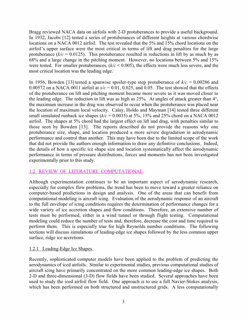
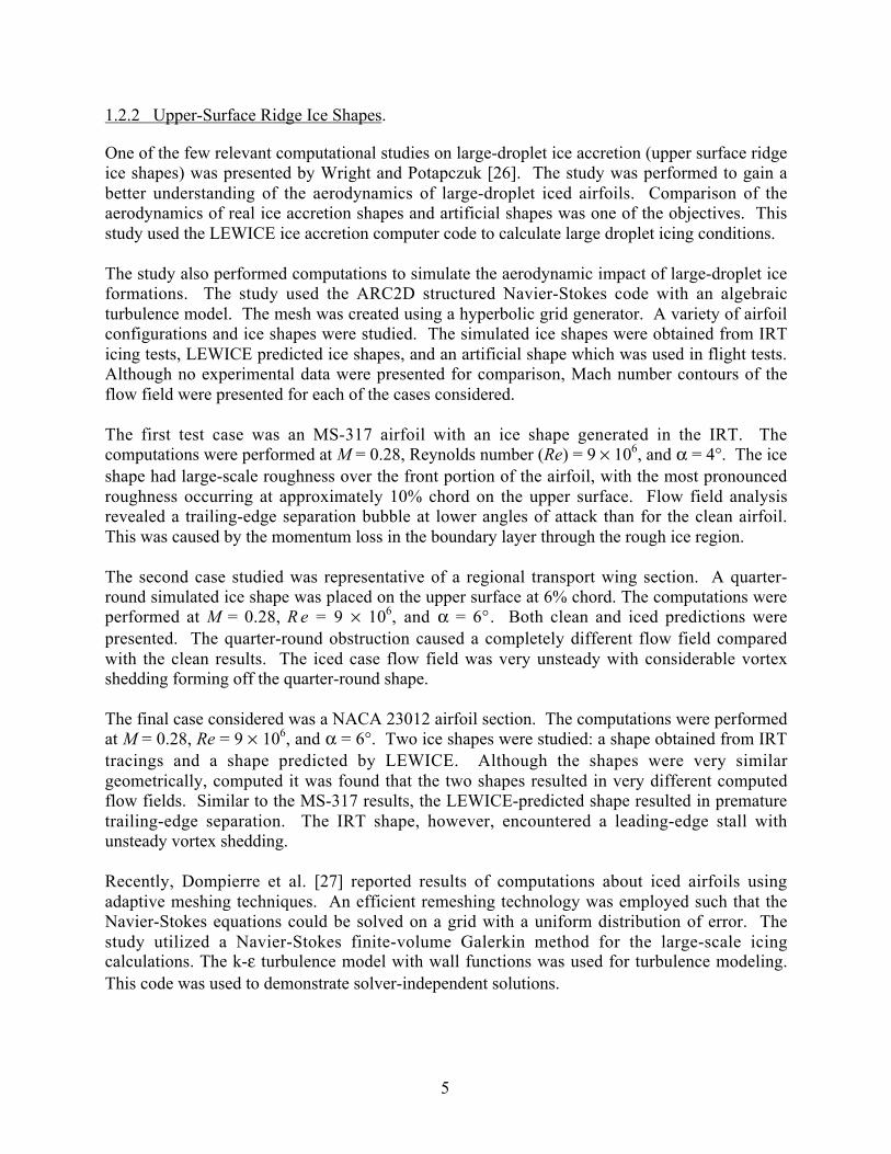
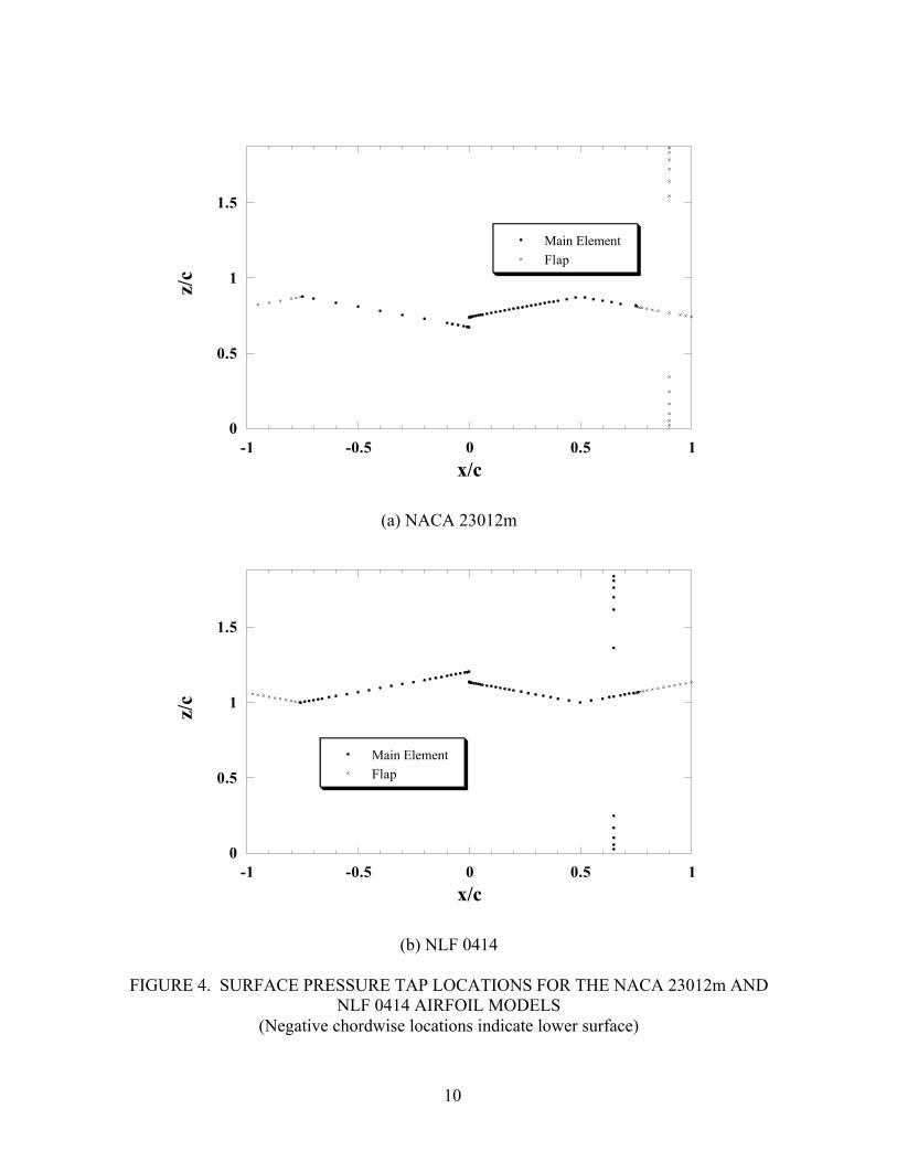
The airfoil models were equipped with surface pressure taps in order to measure the surfacepressure distribution. The NACA 23012m model had 50 surface pressure taps on the mainelement and 30 taps on the flap (including 12 spanwise taps). The NLF 0414 had 75 taps on themain element (including 17 spanwise taps) and 22 taps on the flap. This arrangement is shownin figure 4. The main tap line was angled at 15 degrees with respect to the direction of the flowin order to put the pressure taps out of a possible turbulent wedge generated by the tapspreceding them. The spanwise taps were used to measure spanwise flow nonuniformity near thewalls.

2.1.3 Force and Moment Balance.

An Aerotech three-component force and moment balance (shown in figure 5) was primarily usedto set the model angle of attack. However, it was also used to measure the lift, drag, and pitchingmoment for comparisons to the pressure and wake measurements. The model was mounted onthe metric force plate of the balance with mounting supports. The signals from the load cells onthe balance were gained by a factor of 250, low-pass filtered at 1 Hz and converted to normal,axial, and pitching moment components. The balance did not directly measure lift and dragbecause the load cells turned with the model. The force balance was equipped with a positionencoder that precisely measured the angle of attack. The turntable portion of the balance(including the encoder) was interfaced to the data acquisition computer through the RS-232serial connection. A more detailed description of the force balance can be found in Noe [33].

10

0

0.5

1

1.5

-1 -0.5 0 0.5 1

Main ElementFlap

z/c

x/c

(a) NACA 23012m

0

0.5

1

1.5

-1 -0.5 0 0.5 1

Main ElementFlap

z/c

x/c

(b) NLF 0414

FIGURE 4. SURFACE PRESSURE TAP LOCATIONS FOR THE NACA 23012m ANDNLF 0414 AIRFOIL MODELS

(Negative chordwise locations indicate lower surface)

11

FIGURE 5. THREE-COMPONENT FORCE BALANCE

2.1.4 Flap Actuator and Balance.

The flap was actuated by a two-arm linkage system, which was driven by a Velmex lineartraverse. An Omega LCF-50 load cell with 50 lb range was attached to one of the arms and wasused to measure the flap hinge moments. The traverse was mounted on the metric force plate ofthe force balance. Thus, the entire load on the flap was eventually transferred to the forcebalance.

The flap load cell was calibrated by directly applying loads to the flap by using weights andpulley. The flap was calibrated up to 20 ft-lbs (which was 50% over the maximum moment itwas expected to encounter) with 15 points and was linearly curve fit. The flap was calibrated atfive flap deflection angles (-10, -5, 0, 5, and 10), providing a separate calibration curve for eachflap angle that was to be tested.

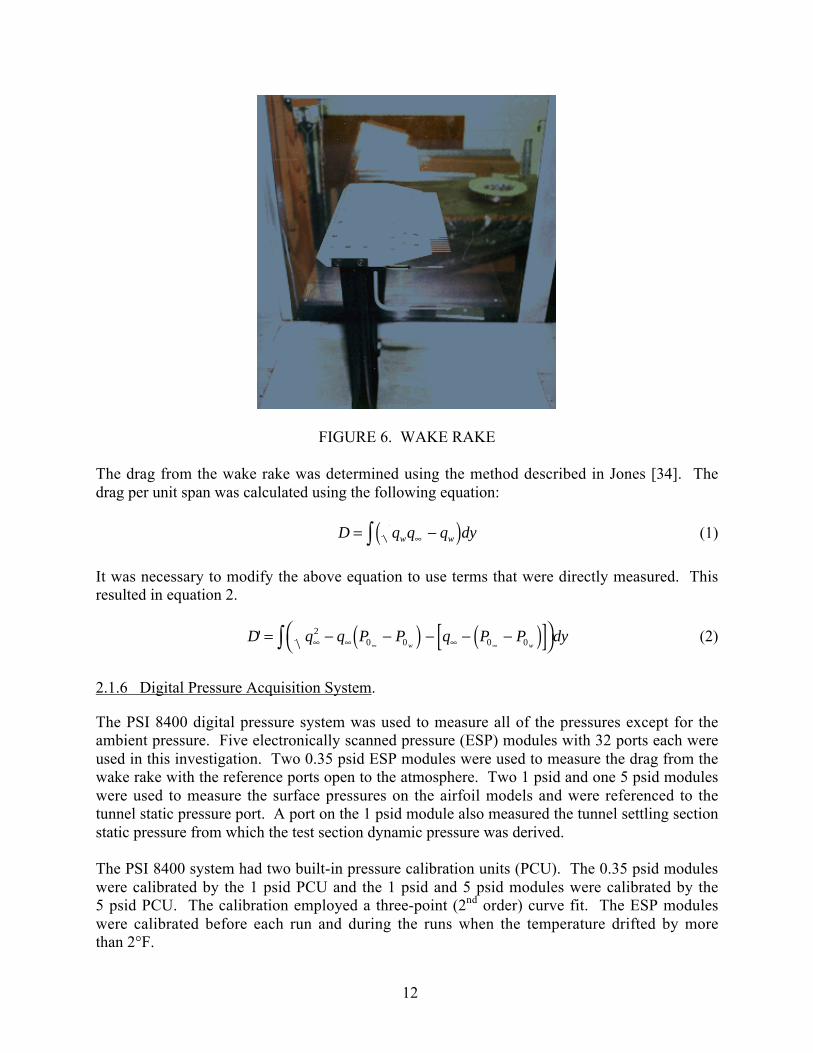
2.1.5 Wake Survey System.

The primary drag measurements were recorded using a wake rake system (figure 6). It contained59 total pressure probes aligned horizontally. The wake rake was traversed by a Velmex traversesystem. The outer six ports on each side of the wake rake were spaced 0.27″ apart and the inner47 ports were spaced 0.135″ apart. The total width of the wake rake was 9.75″. This was wideenough to capture the entire wake when the flow over the model was attached. However, whenthere was a very large wake due to flow separation, two or three spans of the wake rake wereneeded to capture the entire wake. There was a 0.27″ overlap between the successive spans inorder to not to leave any gaps in the wake. The pressures from the wake rake were measuredusing two PSI EPS-32 units with 0.35″ psid range. The total pressures measured from the wakerake were referenced to the atmospheric pressure.

12

FIGURE 6. WAKE RAKE

The drag from the wake rake was determined using the method described in Jones [34]. Thedrag per unit span was calculated using the following equation:

D q q q dyw w= −( )∞∫ (1)

It was necessary to modify the above equation to use terms that were directly measured. Thisresulted in equation 2.

D q q P P q P P dyw w

' = − −( ) − − −( )[ ]

∞ ∞ ∞∞ ∞∫ 2

0 0 0 0 (2)

2.1.6 Digital Pressure Acquisition System.

The PSI 8400 digital pressure system was used to measure all of the pressures except for theambient pressure. Five electronically scanned pressure (ESP) modules with 32 ports each wereused in this investigation. Two 0.35 psid ESP modules were used to measure the drag from thewake rake with the reference ports open to the atmosphere. Two 1 psid and one 5 psid moduleswere used to measure the surface pressures on the airfoil models and were referenced to thetunnel static pressure port. A port on the 1 psid module also measured the tunnel settling sectionstatic pressure from which the test section dynamic pressure was derived.

The PSI 8400 system had two built-in pressure calibration units (PCU). The 0.35 psid moduleswere calibrated by the 1 psid PCU and the 1 psid and 5 psid modules were calibrated by the5 psid PCU. The calibration employed a three-point (2nd order) curve fit. The ESP moduleswere calibrated before each run and during the runs when the temperature drifted by morethan 2°F.

13

2.1.7 Ice Simulation.

The ridge ice accretions were simulated using several basic geometries as shown in figure 7.The baseline ridge ice accretions were simulated with wooden forward-facing quarter-roundshapes of 0.10″, 0.15″, and 0.25″ heights. This geometry was used because it has a vertical stepfacing the flow, which is consistent with the shape of the residual ice that forms just aft of thewing ice protection system in an SLD encounter. The forward-facing quarter round is also thegeometry used by the FAA during aircraft certification. Finally, a simple geometry, such as theforward-facing quarter round, allowed a much easier implementation for the numerical modelingaspect of this investigation.

FIGURE 7. ICE SHAPE SIMULATION GEOMETRY

The other geometries tested consisted of backward-facing quarter round, half round, andforward-facing ramp (all with 0.25″ height and made of wood). The ramp shape was machinedfrom aluminum and had a base length to height ratio of 3. The 0.25″ forward-facing quarterround was also tested with spanwise gaps (the detailed geometry of the spanwise gaps isprovided in the results and discussions section). The simulated ice shapes were attached to themodel using clear Scotch tape.

Roughness was also used both in place of, and in addition to, the simulated ice shape. When itwas used in place of the ice shape, the roughness had a 0.5″ chordwise extent. When used withthe ice shape, the roughness extended upstream and/or downstream from the ice shape. Thechordwise extent of the upstream roughness varied from 0.25″ to 2″, and the extent of thedownstream roughness was 2″. The roughness was simulated using 16-grit aluminum carbideattached to a double-sided tape. This resulted in 0.025″ roughness height, with k/c = 0.0014.The roughness density in terms of the coverage area was estimated to be about 30%.

The 0.25″ height of the baseline shapes was obtained from scaling the actual 0.75″ ridge iceaccretion observed during tanker and icing wind tunnel tests. A survey of various commuter-

Forward-FacingQuarter Round

Backward-FacingQuarter Round

Forward-FacingRamp

Half Round

Direction of Flow

14

type aircraft by the authors showed that the average chord at the aileron section was roughly 5feet [35]. The airfoil models used in the current investigation had 1.5-ft chord. Thus, when theactual 0.75″ ice accretion was scaled by the ratio of the University of Illinois at Urbana-Champaign (UIUC) airfoil model and the full size chord (1.5/5), a scaled height of 0.225″resulted. This was rounded up to 0.25″ to provide a convenient number. Two other heights(0.10″ and 0.15″) were also tested in order to determine the effects of ice accretion height.

For most of the cases tested, the boundary layer was tripped at x/c = 0.02 on the upper surfaceand at x/c = 0.05 on the lower surface. The trip consisted of 0.012-inch-diameter microbeadsthat were applied onto a 0.003-inch-thick and 0.25-inch-wide double-sided tape. The modelswere tripped for two reasons. When the leading-edge deicing boot is activated, it usually doesnot remove all of the ice accretion. Instead, a residual ice roughness is usually left behind whichcauses the flow to be turbulent (or at least transitional) from the leading edge. Another reasonfor the trip was to provide a fixed transition location for the Computational Fluid Dynamics(CFD) simulations. Figure 8 shows the NACA 23012 model with the baseline 0.25″ forward-facing quarter round at x/c = 0.10.

FIGURE 8. NACA 23012 MODEL WITH QUARTER-ROUND ICE SIMULATION(0.25″ quarter round at x/c = 0.10 shown)

2.1.8 Data Acquisition and Reduction.

A typical run consisted of sweeping the angle of attack from negative stall to a few degrees pastpositive stall in 1° increments. At each angle of attack, the flap was swept from -10° to 10° in 5°increments. Before each run, the digital pressure system was calibrated and the force and hingemoment balance tares were measured.

The lift coefficient (Cl) and pitching moment coefficient (Cm) measurements were derived from

both the force balance and the surface pressure measurements. In this report, the Cl and Cm data

were taken from the pressure measurements unless indicated otherwise. The primary dragcoefficient (Cd) measurements were taken with the wake rake and confirmed with the forcebalance. The flap hinge moment coefficients (Ch) were measured with the flap hinge load celland confirmed with the surface pressure measurements. The surface pressure measurements and

15

fluorescent oil flow visualization were used for flow diagnostics. The Cl, Cm, Cd, and Ch values

were calculated using standard methods with conventional definitions:

C

L

q cl =∞

'(3a)

CD

q cd = ′

∞

(3b)

CM

q cm = ′

∞2 (3c)

CH

qhf

= ′

∞c 2(3d)

All of the aerodynamic coefficients were corrected for wall effects using the method describedby Rae and Pope [36].

The surface pressure coefficients were defined as:

Cp p

qp = − ∞

∞

(4)

In addition to providing the lift and pitching moment, the surface pressure measurementsprovided the reattachment locations for small separation bubbles that formed downstream of theice shape simulations. For cases with large separation bubbles, the fluorescent oil flowvisualization method [37] was used for determining the locations of flow reattachment.

All measurements were taken at 50 Hz and averaged over 2 seconds. The force balance datawere low-pass filtered at 1 Hz. None of the other measurements were filtered. Shown in table 1are the uncertainty estimates of the aerodynamic coefficients for a typical data point. The caseshown is that of the clean NACA 23012m model α = 5º with zero flap deflection and Re = 1.8million. The relative uncertainties for Cm and Ch appear to be rather large, but this was due torelatively small reference values at this point.

TABLE 1. EXPERIMENTAL UNCERTAINTIES FOR THE CLEAN NACA 23012m MODELAT α = 5º, Re = 1.8 MILLION

Aerodynamic Reference Absolute RelativeCoefficient Value Uncertainty UncertaintyCl Pressure 0.633 2.11x10-03 0.33%

Cd Wake 0.01022 1.43x10-04 1.40%Cm Pressure -0.00894 3.49x10-04 3.90%Ch Balance -0.0157 3.55x10-03 9.70%

16

2.2 COMPUTATIONAL METHODOLOGY.

The science of CFD has made great strides in recent years. Many new flow solving and gridgenerating techniques have been developed. Tremendous improvements in computingcapabilities have significantly contributed to the field as well. These advancements havefacilitated the solution of many complex flow fields that had been previously impossible. Inparticular, advanced grid generation techniques and high-capacity computers have enhanced ourability to compute flow fields around airfoils with simulated ice shapes.

Most aerodynamic simulations using computational fluid dynamics are performed usingstructured grids. Structured grids are very efficient and are very convenient for conventionalairfoil with attached flow. However, airfoils with complex geometries, such as airfoils withsignificant ice acretions or multielement airfoils, are not easily mapped onto a conventionalstructured grid. One solution to this problem is to use a multiblock structured grid. Thisinvolves tessellating the domain between the body and far field into simple rectangular blocks.The grid can then easily be generated within each block. This process is very difficult toautomate and thus requires much interaction with the user. Another method is using overlapping(chimera) grids. Here, structured grids are generated about each component in the flow field.These grids are allowed to overlap. This method is also difficult to automate, and the flow solverrequires overhead for interpolating between grids.

Recently another solution to this problem has prompted a surge of activity: unstructured grids.Unstructured grids have been very popular for use in solid modeling and structural mechanics formany years. It is only recently that they have received considerable attention within the field offluid dynamics. For use in fluid dynamics, unstructured grids are traditionally composed ofsimplices (triangles in 2-D and tetrahedra in 3-D) and do not possess any coherent structure.Hence, they can provide flexibility for tessellating about 88 complex geometries and adapting toflow features. Generating unstructured grids is also much more automatable than conventionalmultiblock structured grid generation. This allows the user to dedicate much less time to gridgeneration. Although much of the fluid dynamics research using unstructured grids hasconcentrated on inviscid flow problems, recently much progress has been made for highReynolds number viscous flows, which are of much greater practical interest. Currently,unstructured grid technology requires additional memory and computational costs for the samenumber of nodes (often an order of magnitude less). Thus, for complex flows, unstructured gridsare often much more efficient. This, however, is balanced with the ability to compute flowsabout complex geometries and with the ease of adaption, thus, typically requiring fewer nodes.

This chapter describes the various pieces of software that constitute the complete unstructuredCFD package used for the present study. The package was authored and supported by DimitriMavriplis at Scientific Simulations and was based on extensive work completed at NASALangley. It is described in references 38, 39, 40, 41, 42, and 43. The package was developedsuch that the user could proceed step by step, beginning from a simple coordinate description ofthe geometry, and resulting in the fully turbulent steady-state solution of the Navier-Stokesequations about the geometry at the given conditions.

17

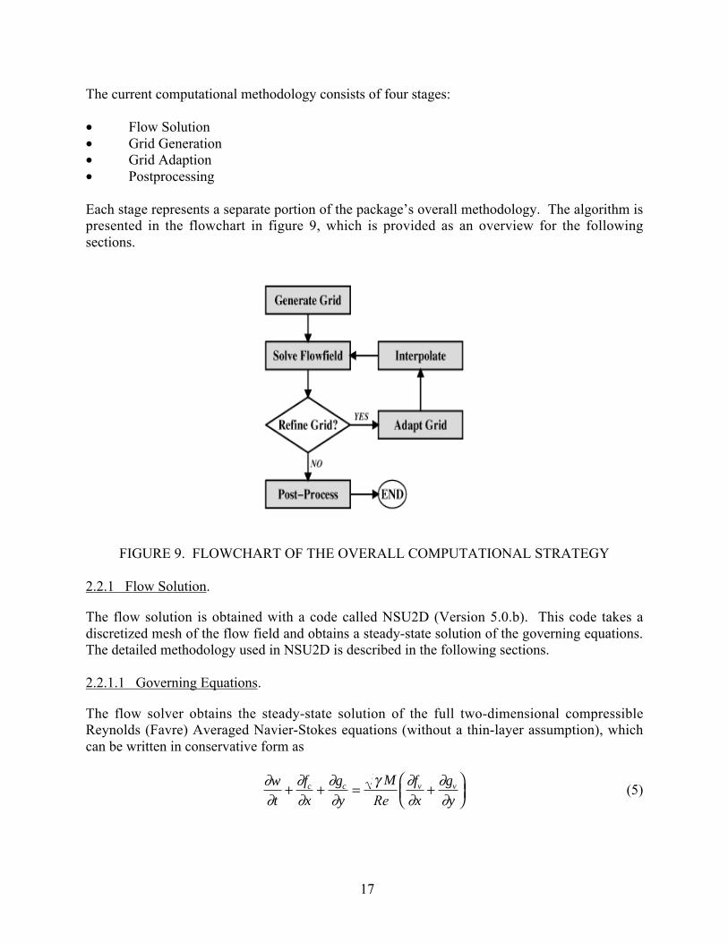
The current computational methodology consists of four stages:

• Flow Solution• Grid Generation• Grid Adaption• Postprocessing

Each stage represents a separate portion of the package’s overall methodology. The algorithm ispresented in the flowchart in figure 9, which is provided as an overview for the followingsections.

FIGURE 9. FLOWCHART OF THE OVERALL COMPUTATIONAL STRATEGY

2.2.1 Flow Solution.

The flow solution is obtained with a code called NSU2D (Version 5.0.b). This code takes adiscretized mesh of the flow field and obtains a steady-state solution of the governing equations.The detailed methodology used in NSU2D is described in the following sections.

2.2.1.1 Governing Equations.

The flow solver obtains the steady-state solution of the full two-dimensional compressibleReynolds (Favre) Averaged Navier-Stokes equations (without a thin-layer assumption), whichcan be written in conservative form as

∂∂

∂∂

∂∂

γ ∂∂

∂∂

w

t

f

x

g

y

M f

x

g

yc c v v+ + = +

Re

(5)

18

where w is the solution vector of the conserved variables

wu

v

E

=

ρρρρ

(6)

and ρ is the fluid density, u and v are the cartesian velocity components, and E is the totalenergy. The pressure, p, can be calculated from the equation of state for a perfect gas

p Eu v

= −( ) −+( )

γ ρ1

2

2 2

(7)

The γ M Re term results from employing the following nondimensional variables

ρ ρρ=

∞

ˆˆ u u

a=

∞

ˆˆ / γ x x

c= ˆ t

tc

a

=∞

ˆ

ˆ / γ

p pp=

∞

ˆˆ

v va

=∞

ˆˆ / γ

y yc= ˆ

where the (∧) denotes dimensional variables, and the infinity (∞) refers to freestream values.Using the components of w along with the pressure, the cartesian components of the convectivefluxes (fc,gc) are given as

f

u

u p

uv

uE up

c =+

+

ρ

ρρ

ρ

2

g

v

vu

v p

vE vp

c =++

ρρ

ρρ

2(8)

and the components of the viscous fluxes (fv,gv) are given by

v

xx

xy

xx xy x

f

u v q

=

+ −

0

σσ

σ σ

v

xy

yy

xy yy y

g

u v q

=

+ −

0

σσ

σ σ

(9)

19

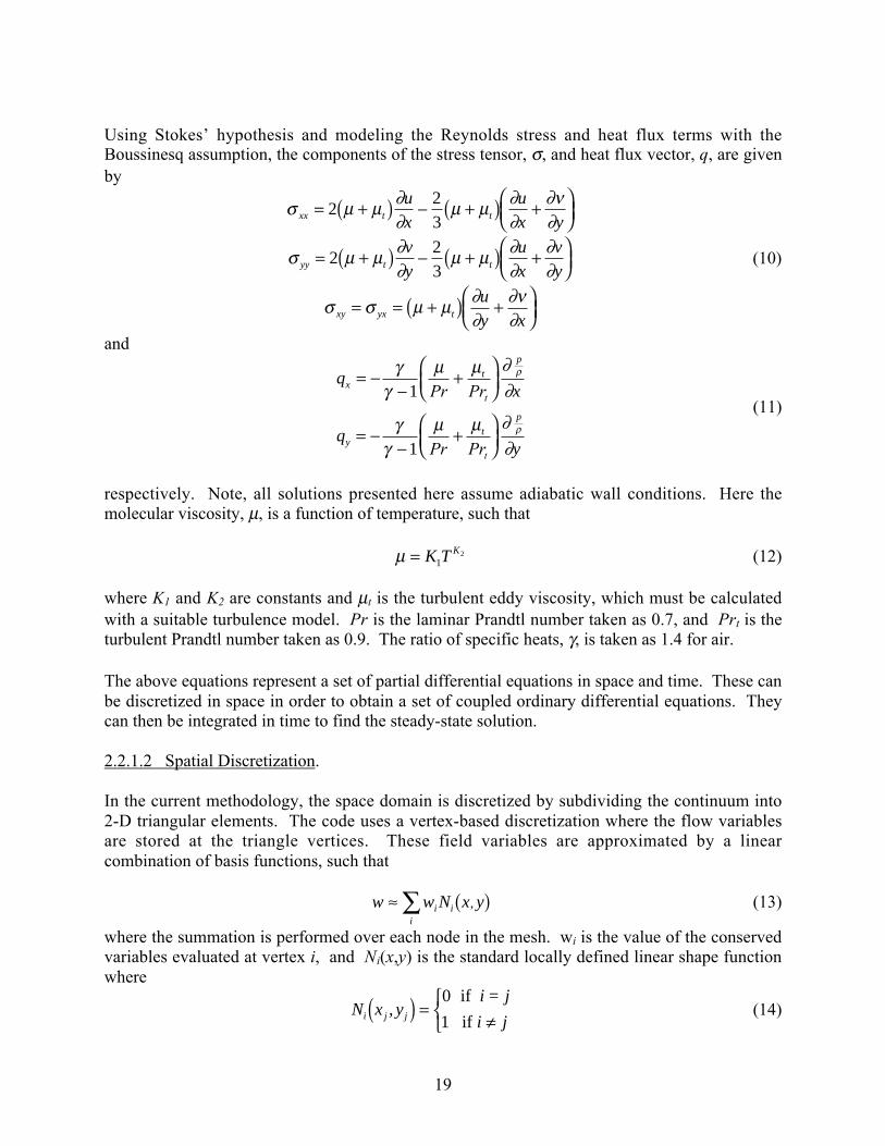
Using Stokes’ hypothesis and modeling the Reynolds stress and heat flux terms with theBoussinesq assumption, the components of the stress tensor, σ, and heat flux vector, q, are givenby

σ µ µ ∂∂

µ µ ∂∂

∂ν∂xx t t

u

x

u

x y= +( ) − +( ) +

223

σ µ µ ∂∂

µ µ ∂∂

∂∂yy t t

v

y

u

x

v

y= +( ) − +( ) +

223

(10)

σ σ µ µ ∂∂

∂ν∂xy yx t

u

y x= = +( ) +

and

qx

qy

xt

p

yt

p

= −−

+

= −−

+

γγ

µ µ

γγ

µ µ

ρ

ρ

1

1

Pr Pr

Pr Pr

t

t

∂∂

∂∂

(11)

respectively. Note, all solutions presented here assume adiabatic wall conditions. Here themolecular viscosity, µ, is a function of temperature, such that

µ = K T K1

2 (12)

where K1 and K2 are constants and µt is the turbulent eddy viscosity, which must be calculatedwith a suitable turbulence model. Pr is the laminar Prandtl number taken as 0.7, and Prt is theturbulent Prandtl number taken as 0.9. The ratio of specific heats, γ, is taken as 1.4 for air.

The above equations represent a set of partial differential equations in space and time. These canbe discretized in space in order to obtain a set of coupled ordinary differential equations. Theycan then be integrated in time to find the steady-state solution.

2.2.1.2 Spatial Discretization.

In the current methodology, the space domain is discretized by subdividing the continuum into2-D triangular elements. The code uses a vertex-based discretization where the flow variablesare stored at the triangle vertices. These field variables are approximated by a linearcombination of basis functions, such that

w w N x yii

i≈ ( )∑ , (13)

where the summation is performed over each node in the mesh. wi is the value of the conservedvariables evaluated at vertex i, and Ni(x,y) is the standard locally defined linear shape functionwhere

N x yi j j,( ) =≠

0

1

if

if

i = j

i j(14)

20

Since the convective fluxes are algebraic functions of the conserved variables, they can also becomputed at the element vertices and vary linearly with the basis functions. However, theviscous terms are functions of the gradients in the conserved variables. Therefore, the gradientsrequired for the stress tensor and the heat flux vector are calculated at the centers of the triangles.These first derivatives are constant over each element and can be computed as

∂∂

∂∂

w

x A

w

xdxdy

Awdy

A

w wy yk k

kk k= ∫∫ = =

+( )∑∫ −( )+

=+

1 1 12

1

1

3

1 (15)

∂∂

∂∂

w

y A

w

ydxdy

Awdx

A

w wx xk k

kk k= ∫∫ = =

+( )∑∫ −( )+

=+

1 1 12

1

1

3

1 (16)

where the summation is performed over the three vertices of the triangle.

The flux terms are evaluated using a Galerkin based finite-element formulation. To derive theGalerkin formulation, equation 5 is first rewritten in vector notation

∂∂

γw

t

M+ ∇ ⋅ = ∇ ⋅F Fc vRe

(17)

Next, a weak formulation is obtained using the method of weighted residuals. This is done bymultiplying the above differential system by a test function, φ, and integrating over the entiredomain

∂∂

φ φγ

φt

wdxdy dxdyM

dxdyΩ Ω Ω∫∫ ∫∫ ∫∫+ ∇ ⋅ = ∇ ⋅F Fc vRe

(18)

Using integration by parts to integrate the flux integrals and neglecting the boundary terms yields

∂∂

φ φγ

φt

wdxdy dxdyM

dxdy= ⋅∇ − ⋅ ∇∫∫∫∫ ∫∫F Fc vΩΩ ΩRe(19)

This equation must be evaluated at each node in the domain. To evaluate the above equation at anode P, the test function is taken as a linear combination of the same basis functions used inequation 13.

φ φ= ( )∑ i ii

N x y, (20)

Therefore, the flux integrals in equation 19 are zero for all elements which do not contain thevertex P. Thus, a domain of influence is defined as the union of all triangles with a vertex P.Knowing that ∇φ is constant over a triangle and each triangle is fully enclosed, the flux integralsover the domain of influence can be evaluated for node P to obtain

21

∂∂

γt

N wdxdy LM

Lp ABe

n

ABe

n

= +( )∑ ⋅ − ∑∫∫ ⋅= =

16 21 1

F F n nCA

CB

veFˆ ˆ

ReΩ (21)

where the summation is over all triangles in the domain of influence. Here LAB refers to thelength of the edge, n is the unit vector normal to the edge, FC

A and FCB are the convective fluxes

computed at vertices A and B respectively, and Fve is the viscous flux over triangle e.

Performing a similar analysis to evaluate the left-hand side of equation 21 results in a coupling ofthe time and space derivatives. This makes the set of equations difficult to solve efficiently.Since time-accuracy is not an issue while computing steady-state solutions, the conservedvariables are set to a constant, wp, over the domain of influence. Therefore, wp can be pulled outof the integral to obtain

Ω p

p

ABe

n

e

n

AB

w

tL n

ML

∂∂

γ= +( ) ⋅ − ⋅

= =∑ ∑1

2

3

21 1

F F F ncA

cB

veˆ ˆ

Re(22)

where Ωp is the surface area of the domain of influence.

For certain conditions, the above formulation can be shown to be equivalent to a finite-volumeformulation. It is also analogous to a central differencing scheme on a structured, quadrilateralmesh. As such, artificial dissipation terms must be incorporated for stability. A blend of aLaplacian and biharmonic operators are used. These simulate the blended second and fourthdifferences commonly used with structured grids. The biharmonic dissipation provides second-order accurate background dissipation in regions of smooth flow. The Laplacian dissipationprovides first-order accurate smoothing in the vicinity of shock waves to reduce numericaloscillations.

2.2.1.3 Time Discretization.

The spatial discretization represented by equation 22 is a set of coupled ordinary differentialequations and can be written as

Ωdw

dtQ w D wp

p p+ ( )[ − ( )] = 0 (23)

where the discrete approximation to the convective and dissipative terms for node P arerepresented by Q(wp) and D(wp) respectively. The dissipative terms contain both the viscousfluxes and the artificial dissipation terms. This set of equations is integrated in time using anexplicit five-stage Runge-Kutta time-stepping scheme given by

22

w w

w wt

Q w D

w wt

Q w D

w wt

Q w D

w wt

Q w D

n

p

p

p

p

0

1 01

00

2 02

11

3 03

22

4 04

3

( )

( ) ( ) ( )

( ) ( ) ( )

( ) ( ) ( )

( ) ( ) ( )

=

= − ( )[ − ]

= − ( )[ − ]

= − ( )[ − ]

= − ( )[ −

α

α

α

α

∆Ω∆Ω∆Ω∆Ω 33

5 05

44

1 5

]

= − ( )[ − ]=

( ) ( ) ( )

+ ( )

w wt

Q w D

w wp

n

α ∆Ω

(24)

where

D D D w

D D D w D

D D w D

0 10

2 3 12

1 0

4 24

2 2

1

1

= = ( )= = ( ) + −( )= ( ) + −( )

( )

( )

( )

β β

β β

and the coefficients are given as

α1 = 1/4 α2 = 1/6 α3 =3/8 α4 = 1/2 α5 = 1

β1 = 0.56 β2 = 0.44

Here wn represents the solution vector at the nth time step, and w(q) represents the solution at theqth stage within the time step. Notice that the convective terms are evaluated at every stage,while the dissipation terms are only evaluated at the first, third, and fifth stages. This schemewas designed to obtain the best balance of efficiency and robustness for viscous flows with thealgebraic multigrid algorithm.

Although the turbulence equations could be integrated in time with this same procedure, it wouldimpose a more restrictive time-step limitation and lead to slower convergence. Since theturbulence equations are only loosely coupled to the governing equations, it is possible to use adifferent integration strategy when solving them. Therefore, the turbulence model is integratedusing a point-implicit or Jacobi iteration strategy. The implicit strategy allows a larger time stepto be used on the turbulence equations than would be possible using an explicit scheme, thereforeallowing the turbulence quantities to be advanced at the same rate as the governing equations.One Jacobi iteration is performed during each stage of the time-stepping scheme. The detailsassociated with the actual method used in NSU2D are described in reference 42.

23

2.2.1.4 Convergence Acceleration Techniques.

The NSU2D program has been primarily designed to obtain steady-state solutions, i.e., time-stepping until all time derivatives are reduced to an acceptably small level. Therefore, the time-accuracy of the solution can be compromised in order to accelerate convergence. Variousconvergence accelerating techniques are used in the code, such as local time-stepping, residualsmoothing, and an algebraic multigrid algorithm.

Local time-stepping advances the equations at each grid point by the maximum permissible time-step at that point as determined by stability analysis. This ensures stability as calculated fromlocal grid and flow properties. Both convective and diffusive characteristics of the Navier-Stokes equations must be considered. Therefore, the local time-step is taken as a weightedcombination of the inviscid and viscous time-step limits

∆ ∆ ∆∆ ∆

t CFLt t

t tc v

c v

=+

(25)

where CFL is the inviscid Courant number. Here

∆ Ωtc

c

=λ

∆ Ωt Kc v

v

=λ

(26)

where Ω denotes the control volume area, Kv is a coefficient which determines the relativeimportance of the viscous and inviscid contribution to the time-step limit, and the eigen valuesare given by

λ

λ γ µρ

c AB AB AB AB AB AB ABe

n

vM

AB ABe

n

U y v x c x y

x yAB

AB

= − + +

+

=

=

∑∑= [ ]

∆ ∆ ∆ ∆

∆ ∆Ω

2 2

1

2 2

1

3 2/

RePr

(27)

The above formulation is a simplified version of the actual method used in NSU2D since thestability of the turbulence equations must also be taken into account.

Residual smoothing is also employed to accelerate convergence by allowing the use of largerCourant numbers and, hence, larger time-steps. Residual smoothing is a technique whichinvolves implicitly averaging the residuals in order to increase the stability limit of thediscretized equations. The original residuals, R, may be replaced by the smoothed residuals, R ,by solving the implicit equation

R R Ri i i= + ∇ε 2 (28)

at each node, i, in the mesh. Here ε is the smoothing coefficient. The above equation is solvedusing an iterative Jacobi scheme.

24

The main technique used in NSU2D to accelerate the convergence is the multigrid algorithm.This method performs time-steps on a sequence of progressively coarser grid levels. Thismethod accelerates convergence by damping out low-frequency errors on the coarser grids wherethese errors can manifest themselves as high frequencies. In the NSU2D methodology, thecoarse grid levels are not physical grids which must be generated separately, rather, they arecreated automatically prior to the flow solution through agglomeration. Here the fine gridcontrol volumes are fused together to form complex polyhedral coarse grid control volumes.NSU2D uses an algebraic multigrid algorithm (AMG), as opposed to a geometric algorithm, andtherefore operates on the matrix of the discrete operator, rather than on the grid of thediscretization. The formulation of the algebraic algorithm can be found in reference 44.

The present research used a W-cycle to traverse the various grid levels during the multigridcycle. Here a time-step is first performed on the finest grid. Then, the flow variables areinterpolated to the next coarser grid, on which a time-step is performed. This process is repeatedrecursively until the coarsest mesh has been reached. The flow solution is then interpolated backto the finer grids and the grid levels are marched in a W pattern.

Five grid levels were typically used for the current computations. However, for grids constrainedby the outer boundary, such as when modeling wind-tunnel walls, fewer grid levels needed to beused since the control volumes of the coarse grid levels were wider than the flow field. Also, forflows with large separation regions, it was found that numerical instabilities developed in thecoarse grid levels, therefore preventing convergence. Reducing the number of grid levelseliminated these instabilities and allowed convergence. For these cases, three grid levels wereused.

2.2.1.5 Turbulence Model.

The NSU2D code supports the computation of inviscid flows, laminar viscous flows, andturbulent viscous flows. For practical flows at large Reynolds numbers, turbulence must besimulated. This is done through an appropriate turbulence model which computes the turbulenteddy viscosity, µt, found in the viscous flux terms of the Reynolds averaged equations (equations10 and 11). There are many eddy-viscosity models in use today. Algebraic turbulence modelssuch as the Baldwin-Lomax [17] model have been very popular for use with structured grids andhave been used for studying iced airfoil aerodynamics [16]. Although it has been done [45],these models are difficult to implement on unstructured grids since the solution at one nodedepends on the solution at neighboring nodes. Therefore, the recent trend is towards simple one-and two-equation models. NSU2D supports the Baldwin-Barth [46] and Spalart-Allmaras [47]one-equation models along with the k-ε (with or without wall functions) [42] and the k-Ω [48]two-equation models. The Spalart-Allmaras model is used exclusively in this research.

The Spalart-Allmaras model has many similarities to the Baldwin-Barth model. However, unlikethe Baldwin-Barth model which was derived from a simplified form of the k − ε model, theSpalart-Allmaras model was developed separately and uses arguments of dimensional analysis,Galilean invariance, and selective dependence on the molecular viscosity. The model iscomputationally local in that the equation at one point does not depend on the solution at otherpoints and is, therefore, well suited for unstructured grids. The model was designed and

25

calibrated for use with mixing layers, wakes, and boundary layers. It therefore appears to be agood candidate for predicting the flow field around iced airfoils. Recently, Spalart et al. [49]modified the original Spalart-Allmaras model to account for system rotation and streamlinecurvature. Although this alteration was found to improve predictions for many types of flows, itwas found to have very little effect on the prediction of backward-facing step flows, which aresimilar to flows encountered around an ice-accreted airfoil. Therefore, the modified version wasnot pursued in this study.

2.2.1.5.1 Description of the Spalart-Allmaras Formulation.

Using dimensional variables for simplicity for the standard Spalart-Allmaras model as describedin reference 50 the kinematic eddy viscosity (νt = µt/ρ) is related to a working variable, ν , by

ν νt vf= ˜1 (29)

where

fcv

v1

3

31

3=+χ

χ(30)

and

χ νν

≡˜

(31)

The working variable, v , obeys the transport equation

D

Dtc S v c c f

db b w w

˜ ˜ ˜ ˜ ˜ ˜˜ν ν

σν ν ν ν= + ∇ ⋅ +( )∇( ) + ∇( )[ ] −

1 2

2

1

21

(32)

Where DDt denotes the substantial derivative and d is the distance to the closest wall. The

quantity S in the production term is given by

˜ ˜S S

dfv≡ + ν

κ 2 2 2 (33)

where the source term, S, is modeled with the magnitude of the vorticity

S

v u

y= ≡ −ω ∂

∂∂∂x

(34)

26

The closure functions appearing in the above equation are defined as

ff

f gc

g c

g r c r r

rS d

vv

ww

w

w

21

36

63

6

1 6

26

2 2

11

1

= −+

= ++

= + −( )≡

χχ

νκ

/

˜˜

(35)

The constants, as specified in reference 47, are given as follows: κ = 0 41. , σ = 2/3, cb1 = 0.1355,

cb2 = 0.622, cv1 = 7.1, c c cw b b1 12

21= + + )(κ σ , cw2 0 3= . , and cw3 2= .

2.2.1.5.2 Transition Specification.

Within the turbulent flow field, the NSU2D code provides a procedure to establish transitionpoints, or more precisely, to define laminar regions which run along the airfoil surface andextend into the flow field. This laminar region is modeled by turning off the source terms in theturbulent transport equations. This produces a laminar effect but does not eliminate thepossibility of turbulent eddy viscosity being convected or diffused into these regions from theneighboring turbulent regions.

Although the code allows prescription of the laminar to turbulent transition location, the codeitself does not predict the location of transition. Therefore, the transition points must be userspecified. In this research the transition points are predicted a priori using the integral boundarylayer program of XFOIL [51]. This program incorporates an eN-type amplification formulationfor determining the transition location. The eN method is based on the Orr-Sommerfeld equationand assumes that transition occurs when the most unstable Tollmien-Schlichting wave in theboundary layer has grown by some factor, taken here as e9. A detailed description of this methodas used in XFOIL can be found in reference 52. To account for variations in the predicted lift ofXFOIL, a lift-corrected angle of attack is used when the transition point is being computed.When comparing against experimental tests which have a boundary layer trip placed on theairfoil, the transition is assumed to occur at which ever comes first: the trip location or thetransition location predicted by XFOIL.

The presence of the quarter-round ice shape on the airfoil required additional consideration whiledetermining whether to model laminar or turbulent flow. The protuberance can cause a largeseparation bubble that will initiate at the top of the shape due to its sharp corner. Thisconfiguration fortunately eliminates the problem of predicting the separation point of the free-shear layer, which can be difficult to accurately simulate on smooth surfaces. For entrainmentalong the free-shear layer itself, the flow can be considered fully developed turbulent in a smallfraction of a step height downstream of the separation point for the Reynolds numbers

27

considered herein [53]. Therefore, the entire free-shear layer and reattachment region weremodeled as turbulent.

All experimental results considered in the icing results (section 4.2) use trip strips placed at 2%chord on the upper surface and 5% chord on the lower surface. Due to the complex geometryand large separation regions, XFOIL cannot accurately predict the flow about an iced airfoil.Therefore, for all positive angles of attack, the upper surface transition point for the iced airfoilwas always taken as the trip location. This is because the iced case was limited to low liftcoefficients such that the lift-corrected non-iced XFOIL transition was never further upstreamthan the trip location. Computations where the upper surface trip location was moved furtherupstream did not change the results significantly. However, for negative angles of attack, thetransition location on the lower surface moved forward of the transition trip. Therefore, thetransition position for the lower surface was taken at the leading edge for all negative angles ofattack.

2.2.2 Grid Generation.

The grid is generated using an interactive program for Silicon Graphics (SGI) workstationscalled UMESH2D (Version 3.0.a). The code creates an unstructured (triangular) discretizationof the entire flow field from an initial coordinate definition of the geometry. The code wasdesigned with emphasis on multielement, high-lift viscous airfoil configurations. The resultinggrid contains highly stretched elements within the boundary layers and wakes and is thereforesuitable for high Reynolds number viscous flows.

The grid is generated in six independent stages:

• Geometry• Wake Generation• Surface Grid Spacing Specification• Interior Grid Spacing Specification• Grid Generation• Mesh Postprocessing and Output

In the first stage, the user provides a pointwise geometry description of the airfoil and allboundaries. Figure 10(a) shows an example geometry definition for a typical three-elementairfoil configuration. Next, a spline curve is generated from these coordinates and a wake isgenerated by a simple panel method (figure 10(b)). Then the boundary point distribution isdetermined as specified in a user-supplied input file, and a field function is created for thespacing within the domain. The actual grid generation is performed in two stages. First asemistructured mesh within the viscous regions near the walls and wakes are discretized with anadvancing-layers algorithm (figures 10(c) and 10(d)). Then the grid within the remaininginviscid regions is generated using an advancing-front Delaunay method (figures 10(e) and10(f)). These two grid generation procedures are described in detail in the following sections.Finally, optional mesh smoothing (using a Laplacian operator) and edge swapping areperformed. In general, edge swapping was not used for this research as it can lead to poorconnectivity in the boundary layer and wake.

28

(a) (b)

(c) (d)

(e) (f)

FIGURE 10. MESH GENERATION STAGES, (a) GEOMETRY, (b) SPLINE AND WAKE,(c) VISCOUS GRID (FAR FIELD), (d) VISCOUS GRID (CLOSEUP),(e) FINAL GRID (FAR FIELD), AND (f) FINAL GRID (CLOSEUP)

2.2.2.1 Commonly Used Grid Generation Techniques.

To understand the techniques used within UMESH2D, it is useful to first examine the advantagesand disadvantages of the more general grid generation algorithms. Two approaches which havereceived much attention in the CFD community are the advancing-front and Delaunaytriangulation techniques.

29

2.2.2.1.1 Advancing-Front Approach.

Advancing-front techniques begin with a discretization of the boundaries as a set of edges whichform the initial front. An edge of the front is selected, then a new triangle is formed with thisedge and a new point or an existing point on the front. The current edge is then removed fromthe front and the new edges are added to the front (or removed if they are hidden). The processstops when all fronts have merged and the domain is covered. New points are selected/positioned such that the new triangle has an optimal size and shape as determined by a fieldfunction. The new point is rejected if it is located near an existing point on the front or if theresulting triangle crosses over an existing front.

The advancing-front method has many advantages. The method usually produces very highquality elements. The operations are all local in nature which reduces round-off error. Also,boundary integrity is guaranteed. Computationally the algorithm is not very complex andrequires low storage since only the front is active.

There are also many disadvantages. Due to the amount of time required to check forintersections and locate near points, the algorithm is not very efficient. The method generatesthe grid one element at a time; whereas, it would be faster to generate one node at a time sincethere are roughly twice as many triangles as nodes. The method also runs into robustnessproblems caused by the merging fronts.

2.2.2.1.2 Delaunay Triangulation Approach.

Strictly speaking, a Delaunay triangulation is not a grid generation procedure but merely refers toa unique triangulation of a set of points which exhibits well-defined properties. TheBowyer/Watson algorithm is one of the most common sets of properties. It states that no trianglein the Delaunay triangulation can contain a point other than its own three vertices within itscircumcircle. This gives rise to what is known as a point insertion scheme. This type ofalgorithm is useful when the mesh points have been predetermined. An initial mesh whichcompletely covers the entire domain is created. Given this initial triangulation, new points maybe inserted one at a time by locating and deleting all existing triangles whose circumcirclescontain the newly inserted point. New triangles are then formed with the new point.

There are many advantages to such a scheme. It is a very simple algorithm since there are nocomplex data structures associated with locating neighboring points and fronts. The mesh isgenerated point by point, rather than one triangle at a time.

There are also some disadvantages to this type of scheme. The final mesh does not have theelement quality and the grid is not as smooth as grids generated by advancing-front methods.During the insertion process, nonlocal operations may be required which can lead to round-offerrors. Also, boundary integrity is not guaranteed.

2.2.2.2 Grid Generation Techniques Used in UMESH2D.

Grid generation within UMESH2D is separated into two stages. First the viscous mesh isgenerated, then the rest of the mesh is filled in. The algorithms used are described in thefollowing sections.

30

2.2.2.2.1 Viscous Grid GenerationAdvancing-Layers Method.

The first phase of the grid generation process utilizes the advancing-layers method as describedby Pirzadeh [54]. This stage creates a highly stretched semistructured grid within the viscousregions around the airfoil geometry and wakes. This method is based on the advancing-fronttechnique, and as such, it tries to keep many of the desirable features: a high degree offlexibility, robustness, and good grid quality. As in the standard advancing-front method, gridcells begin from the boundaries and march into the domain. However, unlike the conventionalmethod where individual cells are added in no particular order, the advancing-layers methodadvances an entire layer at a time. This minimizes front congestion, minimizes complexity ofsearch-and-check operations, evenly distributes cells on all solid boundaries as much as possible,provides less complicated operation, and improves efficiency.

To ensure high grid quality, new grid points are positioned along a set of predetermined vectorswhich are normal to the boundary surfaces. The distribution along the vectors is prescribed by astretching function. As the positions of the new points are determined, they are added anddeleted from the current front in a method which is similar to the standard advancing front. Thelayers continue to form and advance until two opposing fronts approach or grid quality becomesunacceptable. In order to control how far the layers advance into the field, a background spacingfunction is used. The advancing process for a face terminates when the local characteristics ofthe grid no longer match the background spacing function. The current front is then stored andused as the initial front for the next stage in the grid generation process. The grid resulting fromthis stage in the grid generation process is seen in figures 10(c) and 10(d). Notice that the gridhas been generated around each airfoil element and the wake regions. Note that although themesh is composed of unstructured triangular elements, the grid in this region is generated in asemi-structured manner, as is evident in the rows and columns of node points.

2.2.2.2.2 Inviscid Grid GenerationAdvancing-Front Delaunay Triangulation Method.

The second phase of the grid generation process uses the method of Mavriplis. This stagecreates isotropic elements within the inviscid regions of the flow field. This hybrid technique isessentially an advancing-front algorithm which adds new points ahead of the front andtriangulates them using the Delaunay criterion. It therefore combines the efficiency andmathematical elegance of Delaunay triangulation with the point placement features, robustness,and boundary integrity of the advancing-front method.

Similar to the standard advancing-front technique, the current methodology begins with an initialset of edges which forms a front. An edge along the front is selected. If none of the pointslocated on the front can combine with the selected edge to form an acceptable Delaunay trianglethen a new point is created. The new point is inserted along the median of the edge at a distancewhich results in the desired circumradius. A field function is used to determine the maximumallowable circumradius for a triangle as a function of its position. This point is then checked tomake sure that it does not lie inside an existing triangle’s circumcircle or violate the boundary. Ifthe point is acceptable then an appropriate Delaunay triangulation is formed with the surroundingpoints. Another edge along the front is then selected, and the process continues until the entiredomain has been discretized. The resulting grid (after smoothing) is shown in figures 10(e) and

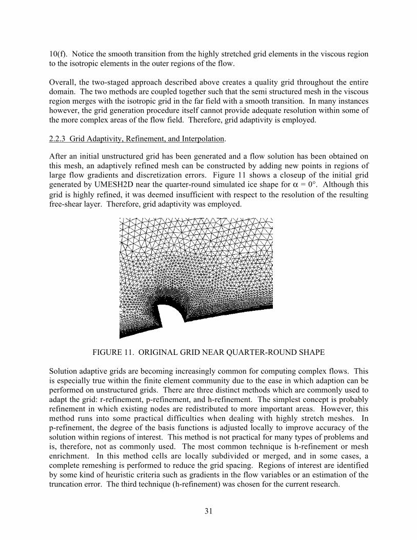
31

10(f). Notice the smooth transition from the highly stretched grid elements in the viscous regionto the isotropic elements in the outer regions of the flow.

Overall, the two-staged approach described above creates a quality grid throughout the entiredomain. The two methods are coupled together such that the semi structured mesh in the viscousregion merges with the isotropic grid in the far field with a smooth transition. In many instanceshowever, the grid generation procedure itself cannot provide adequate resolution within some ofthe more complex areas of the flow field. Therefore, grid adaptivity is employed.

2.2.3 Grid Adaptivity, Refinement, and Interpolation.

After an initial unstructured grid has been generated and a flow solution has been obtained onthis mesh, an adaptively refined mesh can be constructed by adding new points in regions oflarge flow gradients and discretization errors. Figure 11 shows a closeup of the initial gridgenerated by UMESH2D near the quarter-round simulated ice shape for α = 0°. Although thisgrid is highly refined, it was deemed insufficient with respect to the resolution of the resultingfree-shear layer. Therefore, grid adaptivity was employed.

FIGURE 11. ORIGINAL GRID NEAR QUARTER-ROUND SHAPE

Solution adaptive grids are becoming increasingly common for computing complex flows. Thisis especially true within the finite element community due to the ease in which adaption can beperformed on unstructured grids. There are three distinct methods which are commonly used toadapt the grid: r-refinement, p-refinement, and h-refinement. The simplest concept is probablyrefinement in which existing nodes are redistributed to more important areas. However, thismethod runs into some practical difficulties when dealing with highly stretch meshes. Inp-refinement, the degree of the basis functions is adjusted locally to improve accuracy of thesolution within regions of interest. This method is not practical for many types of problems andis, therefore, not as commonly used. The most common technique is h-refinement or meshenrichment. In this method cells are locally subdivided or merged, and in some cases, acomplete remeshing is performed to reduce the grid spacing. Regions of interest are identifiedby some kind of heuristic criteria such as gradients in the flow variables or an estimation of thetruncation error. The third technique (h-refinement) was chosen for the current research.

32

Unlike most of the software used in this research, the code used to generate adaptive grids wasdeveloped in-house. The grid refinement was performed by splitting edges in regions of highflow field gradients. If the gradient of a particular flow variable was larger than some prescribedtolerance, the edge was refined by adding a new point at the midpoint of the edge. Pressuregradients render good refinement of the inviscid flow features, such as shocks and expansions.Gradients in velocity and Mach number provide good refinement of the viscous phenomenawithin boundary layers, wakes, and shear layers. The refinement criteria was based on a first-order approximation to the error and was calculated along each edge from the flow variablegradients within each element. The error along an edge was taken as the average of themagnitude of the gradient for the two neighboring elements multiplied by the edge length. Thetechnique essentially subdivides the elements with the largest flow field gradients. Thisapproach is similar to the method of Mavriplis [42] which bases refinement on the undivideddifference along an edge.

Figure 12 shows the grid resulting from one adaptation based on gradients in absolute velocity.Figure 13 shows the corresponding velocity contours of the initial solution. Note that additionalgrid points have been clustered around the separation point and along the high-velocity gradientsof the downstream free-shear layer. The adaption increased the number of grid points byapproximately 25%. It should be noted that in the present methodology, elements near the airfoiland within the boundary layer are not subdivided. This was done to limit the overall number ofpoints and still allow adequate resolution within the shear layer. All computations with ridge iceshapes presented in section 4.2 used this same adaption strategy. Using additional refinementand adaption was also investigated, but there were no significant differences in flow prediction.

FIGURE 12. ADAPTED GRID NEAR QUARTER-ROUND SHAPE

33

FIGURE 13. ABSOLUTE VELOCITY CONTOURS FOR ORIGINAL GRID

After the grid has been refined, a new flow field solution is obtained on the new adapted grid.To reduce the number of time cycles required for convergence, it is desirable to initialize theflow field with the previously computed solution. This is accomplished with a simpleinterpolation procedure from the original grid to the new grid by using shape functions. Thedifficulty lies in the determination of the coarse grid cell that encloses a particular fine grid node.A naïve search over all the coarse grid cells would require O(n2) operations, where n is on theorder of the number of fine grid nodes and the number of coarse grid cells. This would beimpractical since it would require more time to perform the search than it would take to computethe flow solution. Therefore, a more efficient search method is needed. This is accomplished inthe current research by using a neighbor search. Interpolation to the adapted-grid node, N1, isinitiated by providing an initial guess, E1, for the coarse grid element. This cell is then tested byits shape functions to see if it encloses N1. If the test is positive, then the values at the vertices ofare interpolated to N1. If the test is negative, then the neighboring cell of E1 with a centroid,which is closest to N1, is the next cell tested. The algorithm then marches through the coarse griduntil the enclosing cell is found. In many cases this strategy can run into problems with complexdomains and boundary conditions. Therefore, the search must be checked to make sure that it isnot going in circles. If this is the case, then a brute force check of all the coarse grid cells isperformed for the current node. In some rare cases due to grid smoothing and point placementalong the boundary, a node in the fine grid will actually lie outside the coarse grid domain, i.e.,there is no enclosing cell. In this case, the closest coarse grid node is located and the flowvariables are copied to the fine grid node.

2.2.4 Postprocessing and Data Reduction.

After the flow solution has been obtained, the solution is analyzed to determine the aerodynamicproperties of the airfoil. The lift, drag, and moment coefficients are calculated by integrating thesurface pressure and skin friction about the entire airfoil while the hinge moment coefficient isintegrated about the flap only. Most experimental data presented here for comparison measurethe momentum loss through the tunnel test section with a wake pressure survey to obtain the total(viscous and pressure) drag on the airfoil. The surface pressure taps are used to measure the

34

experimental lift and moment coefficients, and thus only include the inviscid force contributions.However, in the computational results, viscous forces are included in all force calculations. Thisis not expected to greatly influence the values of these coefficients. The shear stress at the wallused to calculate the skin friction is calculated using a linear approximation to the velocityderivative as determined from the first grid point normal to the airfoil surface. The referencelength used to calculate the lift, drag, and moment coefficients is taken as the airfoil chordlength. The hinge moment uses the flap chord length as the reference length. The pitchingmoments are taken about the quarter-chord location, and the hinge moments are taken about theflap’s pivot location.

3. VALIDATION.

3.1 NACA 23012 COORDINATE MODIFICATION.

As stated in the previous section, the NACA 23012 airfoil that was used in this experiment didnot have coordinates that are conventionally defined. The airfoil coordinates were generatedthrough XFOIL [51] by selecting the standard NACA 23012 configuration. However, XFOILgenerates thicknesses on a vertical plane instead of normal to the mean camber line, producing asmall difference near the leading edge as compared to a conventionally defined NACA 23012.The result was a slightly drooped leading edge with a maximum vertical coordinate shift of 0.4%chord as compared to the conventional NACA 23012. In addition, because of errors in themanufacture of the model, the maximum was 12.2% instead of the standard 12%. Thecoordinates for the standard NACA 23012 and the modified NACA 23012m (as measured usinga digital coordinate measurement machine) are shown in table 2. The leading edge geometrycomparisons between the modified NACA 23012m and the standard NACA 23012 is shown infigure 14. Because of these differences, the airfoil model used in this study will be called NACA23012m.

The slight change in the airfoil geometry did not significantly alter the airfoil aerodynamiccharacteristics. Figure 15 shows the lift curve comparison between the two airfoils. The resultswere obtained from XFOIL with both of the airfoils at the Reynolds number of 1.8 million. Itshows nearly identical values of Cl,max in the linear region of the lift curve. The NACA 23102m

had a slightly higher Cl,max (1.61) when compared to the standard NACA 23012 (1.57) due to

increased camber.

Figure 16 shows the surface pressure distribution comparisons (again obtained using XFOIL atRe = 1.8 million). It shows nearly identical surface pressure distributions at angles of attack of0° and 5°. At α = 5°, both the modified and the standard NACA 23012 surface pressuredistributions contained a discontinuity between 15% and 20% chord which was caused by alaminar separation bubble. At α = 10° (where the lift curve started to become nonlinear), therewere greater differences in the surface pressure distributions. The modified NACA 23012mairfoil had a Cp,min of -4 while the standard NACA 23012 had a Cp,min of -4.8. Also, the laminarseparation bubble on the modified NACA 23012m is located near x/c = 0.10 while on thestandard NACA 23012, it is located near x/c = 0.06. Figures 15 and 16 show that although themodification of the airfoil geometry cause changes in aerodynamic characteristics, they were notlarge and the distinctive aerodynamic characteristics of the NACA 23012 were maintained.

35

TABLE 2. STANDARD NACA 23012 AND MODIFIED NACA 23012m COORDINATES

Standard NACA 23012 Modified NACA 23012Upper Surface Lower Surface Upper Surface Lower Surface

x/c y/c x/c y/c x/c y/c x/c y/c0 0 0.00533 -0.01 0.00001 0.00037 0.00008 0

2E-04 0.00956 0.01557 -0.01 0.00011 0.00182 0.00017 00.006 0.0203 0.03029 -0.02 0.00094 0.00555 0.00054 00.019 0.03176 0.04915 -0.02 0.0017 0.00756 0.00117 -0.010.037 0.04324 0.07195 -0.03 0.00358 0.01142 0.00206 -0.010.062 0.05382 0.09868 -0.03 0.00381 0.01181 0.00337 -0.010.092 0.06265 0.12954 -0.03 0.00765 0.01738 0.00448 -0.010.127 0.06915 0.16483 -0.04 0.01109 0.02136 0.00567 -0.010.166 0.0732 0.20483 -0.04 0.01512 0.02536 0.00662 -0.010.207 0.07524 0.24869 -0.04 0.01961 0.02926 0.00716 -0.010.251 0.07597 0.29531 -0.04 0.02902 0.03613 0.00851 -0.010.298 0.07554 0.34418 -0.05 0.0347 0.03971 0.00989 -0.010.347 0.07402 0.39476 -0.04 0.03892 0.04217 0.01142 -0.020.397 0.0715 0.4465 -0.04 0.04236 0.04404 0.01308 -0.020.449 0.06811 0.49883 -0.04 0.05899 0.05188 0.01486 -0.020.501 0.06397 0.55117 -0.04 0.06478 0.05419 0.01584 -0.020.553 0.05924 0.60296 -0.04 0.07189 0.05679 0.02046 -0.020.605 0.05405 0.6536 -0.03 0.08701 0.06153 0.02497 -0.020.655 0.04854 0.70257 -0.03 0.09457 0.06356 0.0315 -0.020.704 0.04285 0.7493 -0.03 0.10486 0.06598 0.03617 -0.020.751 0.03712 0.7933 -0.02 0.11263 0.06757 0.04206 -0.020.794 0.03145 0.83407 -0.02 0.12141 0.06912 0.04908 -0.020.835 0.02597 0.87118 -0.02 0.12857 0.07023 0.05754 -0.030.872 0.02079 0.9042 -0.01 0.15473 0.07333 0.05988 -0.030.905 0.01602 0.93279 -0.01 0.16089 0.07388 0.06545 -0.030.933 0.01176 0.95661 -0.01 0.16252 0.07402 0.07327 -0.030.957 0.00812 0.97543 0 0.18336 0.07541 0.07788 -0.030.976 0.00518 0.98901 0 0.19975 0.07612 0.08615 -0.030.989 0.00302 0.99722 0 0.22696 0.07678 0.08891 -0.030.997 0.0017 0.99997 0 0.24468 0.07691 0.09796 -0.03

1 0.00126 0.26005 0.07687 0.10523 -0.030.27779 0.07666 0.11551 -0.030.31478 0.07576 0.11988 -0.030.35461 0.07419 0.1268 -0.030.37689 0.07311 0.13376 -0.030.40376 0.07162 0.14312 -0.040.42647 0.07021 0.15183 -0.040.49844 0.06467 0.16268 -0.040.55317 0.05977 0.18158 -0.04

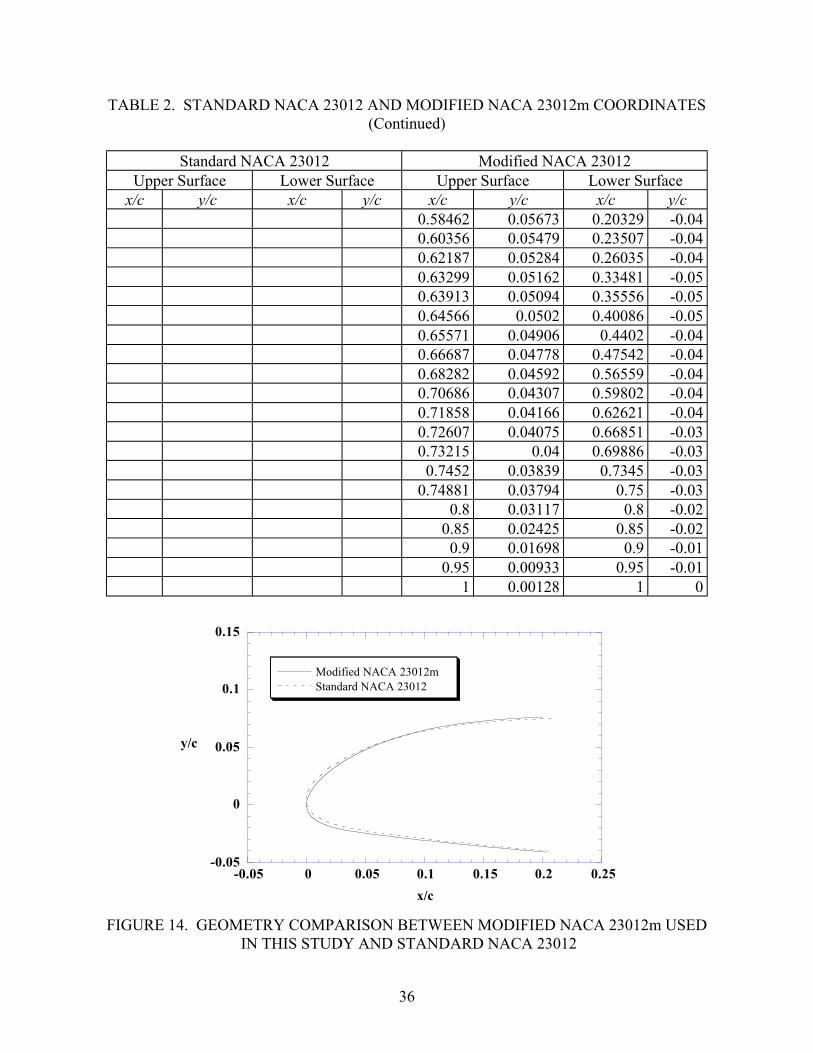
36

TABLE 2. STANDARD NACA 23012 AND MODIFIED NACA 23012m COORDINATES(Continued)

Standard NACA 23012 Modified NACA 23012Upper Surface Lower Surface Upper Surface Lower Surface

x/c y/c x/c y/c x/c y/c x/c y/c0.58462 0.05673 0.20329 -0.040.60356 0.05479 0.23507 -0.040.62187 0.05284 0.26035 -0.040.63299 0.05162 0.33481 -0.050.63913 0.05094 0.35556 -0.050.64566 0.0502 0.40086 -0.050.65571 0.04906 0.4402 -0.040.66687 0.04778 0.47542 -0.040.68282 0.04592 0.56559 -0.040.70686 0.04307 0.59802 -0.040.71858 0.04166 0.62621 -0.040.72607 0.04075 0.66851 -0.030.73215 0.04 0.69886 -0.030.7452 0.03839 0.7345 -0.03

0.74881 0.03794 0.75 -0.030.8 0.03117 0.8 -0.02

0.85 0.02425 0.85 -0.020.9 0.01698 0.9 -0.01

0.95 0.00933 0.95 -0.011 0.00128 1 0

-0.05

0

0.05

0.1

0.15

-0.05 0 0.05 0.1 0.15 0.2 0.25

Modified NACA 23012mStandard NACA 23012

y/c

x/c

FIGURE 14. GEOMETRY COMPARISON BETWEEN MODIFIED NACA 23012m USED IN THIS STUDY AND STANDARD NACA 23012

37

-1.5

-1

-0.5

0

0.5

1

1.5

2

-15 -10 -5 0 5 10 15 20

Modified NACA 23012mStandard NACA 23012

Cl

α (°)

FIGURE 15. LIFT COMPARISON BETWEEN MODIFIED NACA 23012m USED IN THISSTUDY AND STANDARD NACA 23012, RESULTS FROM XFOIL, Re = 1.8 × 106

-5

-4

-3

-2

-1

0

10 0.2 0.4 0.6 0.8 1

α = 0°α = 5°α = 10°

α = 0°α = 5°α = 10°

Cp

α (°)

ModifiedNACA 23012m

StandardNACA 23012

FIGURE 16. SURFACE PRESSURE COMPARISON BETWEEN MODIFIEDNACA 23012m USED IN THIS STUDY AND STANDARD NACA 23012,

RESULTS FROM XFOIL, Re = 1.8 × 106

38

3.2 EXPERIMENTAL VALIDATION.

The clean baseline measurements were taken and compared to previously published data in orderto validate the experimental apparatus and data reduction methods in figure 15. Themeasurements were also compared to the results from XFOIL [51], an airfoil analysis code thatuses an integral boundary element method. The present UIUC data were obtained at a Reynoldsnumber of 1.8 million. Figure 17(a) shows the lift curve comparisons, which indicate goodagreement between the present UIUC experiment and Stuttgart data [55] (taken at Re = 2million). The data of Abbott and von Doenhoff [56] showed a Cl,max that was approximately 8

percent higher which may have been due to their higher Reynolds number (Re = 3 million). Allof the experimental data showed leading-edge stall, as expected for the NACA 23012 airfoil.XFOIL, which was not designed to predict large separated flow regions, showed a more gradualstall and a higher Cl,max.

Figure 17(a) shows that end-wall effects were not significant as there was good agreementbetween the pressure data (which measured lift only near the model mid-chord) and the balancedata (which measured the lift over the entire model). Had there been a significant wall-induced3-D effect, the pressure and the balance data would have differed by a greater amount. Thisconsistency was also verified by flow visualization, which showed that significant 3-D flow wasnot present until past stall. This is in agreement with the significant difference in the pressureand balance data only after stall at α = 17°.

Figure 17(b) shows the drag comparisons. It shows slightly higher drag values for the UIUCdata that may have been due to the flap gap discontinuity and leakage. Figure 17(c) showsreasonable pitching moment comparisons. No previous experimental results were found for flaphinge moment comparisons. Also, XFOIL cannot handle multielements and typically losesaccuracy when predicting the thick boundary layer near the trailing edge; therefore, it was notused to generate a Ch. Thus, figure 17(d) shows only the comparison between the UIUC pressureand flap hinge balance data that agreed reasonably well.

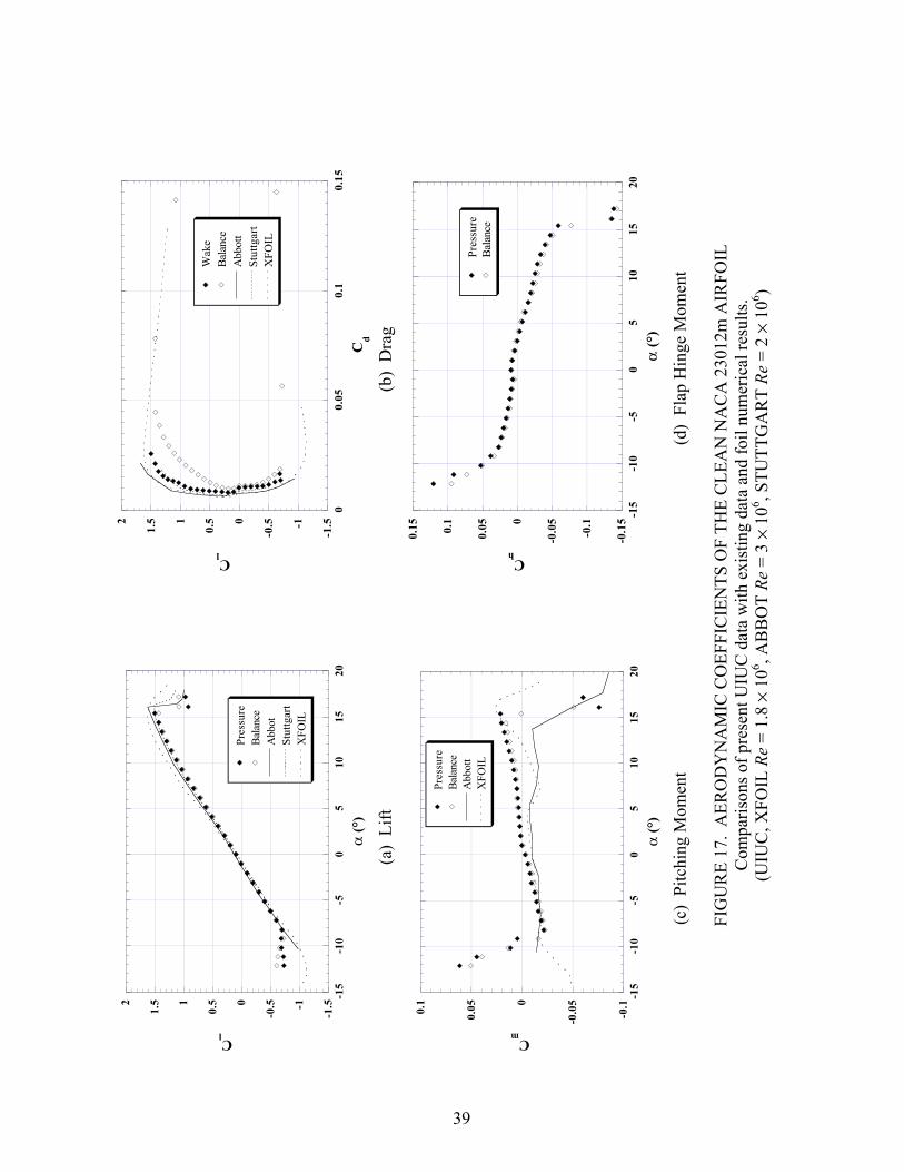
39

-1.5-1

-0.50

0.51

1.52 -1

5-1

0-5

05

1015

20

Pre

ssur

eB

alan

ceA

bbot

Stu

ttga

rtX

FOIL

Cl

α (

°)

-1.5-1

-0.50

0.51

1.52

00.

050.

10.

15

Wak

eB

alan

ceA

bbot

tS

tutt

gart

XFO

IL

Cl

Cd

(a

) L

ift

(b)

Dra

g

-0.1

-0.0

50

0.050.

1 -15

-10

-50

510

1520

Pre

ssur

eB

alan

ceA

bbot

tX

FOIL

Cm

α (

°)

-0.1

5

-0.1

-0.0

50

0.050.

1

0.15

-15

-10

-50

510

1520

Pre

ssur

eB

alan

ce

Ch

α (

°)

(c)

Pitc

hing

Mom

ent

(d)

Fla

p H

inge

Mom

ent

FIG

UR

E 1

7. A

ER

OD

YN

AM

IC C

OE

FFIC

IEN

TS

OF

TH

E C

LE

AN

NA

CA

230

12m

AIR

FOIL

Com

pari

sons

of

pres

ent U

IUC

dat

a w

ith e

xist

ing

data

and

foi

l num

eric

al r

esul

ts.

(UIU

C, X

FOIL

Re

= 1.

8 ×

106 , A

BB

OT

Re

= 3

× 10

6 , ST

UT

TG

AR

T Re

= 2

× 10

6 )

40

Figure 18 shows the comparison between the experimental surface pressures and those predictedby XFOIL. The angles of attack for the experimental data and XFOIL were different by asmuch as 1°. This was done in order to match Cl because XFOIL overpredicted lift, as shown in

figure 17(a). At the matched lift coefficients, the surface pressure agreed reasonably well,including the location of the laminar separation bubble at Cl = 0.65 (located at x/c = 0.19).

-4

-3

-2

-1

0

10 0.2 0.4 0.6 0.8 1

α = -0.24°α = 4.58°α = 9.03°

α = -0.01°α = 4.99°α = 9.99°

Cp

x/c

Cl = 0.10

Cl = 0.65

Cl = 1.18

XFOIL Experimental

FIGURE 18. SURFACE PRESSURE OF THE CLEAN NACA 23012m AIRFOIL.Comparisons of experimental data and XFOIL at matched lift coefficients.

3.3 CODE VALIDATION.

Validation is the process of determining the degree to which a model is an accuraterepresentation of the real world from the perspective of the intended uses of the model. The flowfield about an iced airfoil contains many complicated flow features which are coupled in a verycomplex system. These complexities include Reynolds number effects, Mach number effects,separated flow features, adverse pressure gradient effects, etc. Therefore, it is important tounderstand the computational capabilities of the code with respect to predictive performance ofthe individual complexities of the code, with respect to predictive performance of the individualcomplexities of the system. Therefore, before results could be obtained for the primary icingstudy, a validation study was conducted to become acquainted with the code and determine thecapabilities and limitations of the current computational methodology for each of the primaryflow features. Once there is confidence in the solution for the individual flow physics, then thesystem can be analyzed as a whole more effectively and with greater confidence. In thefollowing section, specific flow features which are consistent with the expected iced-airfoil flowfield are analyzed individually and validated by comparison to theoretical or experimental data.

41

3.3.1 Simple Geometry Flow Field Simulation.

3.3.1.1 Flat-Plate Boundary Layer.

To assess the accuracy of NSU2D within the viscous regions near the wall boundaries, the codeis first verified for a flat-plate boundary layer. This was done to determine an adequate level ofgrid resolution which was required near the airfoil surface. The NSU2D results were comparedwith analytical data obtained from classical incompressible flat-plate boundary layer analysis asfound in White [57]. The compressible calculations were performed at a Mach number of 0.2, socompressibility effects are not expected to greatly influence the solution.

Since the code was designed to analyze airfoil configurations, the flat plate was modeled as athin, flat airfoil. The thickness of the plate was 1% of the length, and the leading edge had anelliptical shape with an aspect ratio of 10:1. The trailing edge was modeled with a sharp drop-off. The total grid contained approximately 30,000 nodes, and the first node in the directionnormal to the airfoil surface was located at approximately a y/c of 1 × 10-6 with a 15% successiveincrease in grid size away from the wall. This places the first grid point in the y + < 1 region forthe turbulent simulations performed, where yet is the nondimensional wall unit of the laminarsublayer.

The following sections present a small selection of the computations performed on the flat plate.A number of grid spacings were tested at a variety of Reynolds numbers for both laminar andturbulent flows. The results presented are considered representative of the findings.

0.0 0.5 1.0

u/ue

0.0

2.0

4.0

6.0

η

BlasiusNSU2D

FIGURE 19. STREAMWISE VELOCITY IN LAMINAR BOUNDARY LAYER INTERMS OF SIMILARITY COORDINATES

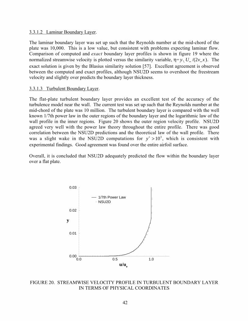
42

3.3.1.2 Laminar Boundary Layer.

The laminar boundary layer was set up such that the Reynolds number at the mid-chord of theplate was 10,000. This is a low value, but consistent with problems expecting laminar flow.Comparison of computed and exact boundary layer profiles is shown in figure 19 where thenormalized streamwise velocity is plotted versus the similarity variable, η= y U v x∞ ∞/( )2 . Theexact solution is given by the Blasius similarity solution [57]. Excellent agreement is observedbetween the computed and exact profiles, although NSU2D seems to overshoot the freestreamvelocity and slightly over predicts the boundary layer thickness.

3.3.1.3 Turbulent Boundary Layer.

The flat-plate turbulent boundary layer provides an excellent test of the accuracy of theturbulence model near the wall. The current test was set up such that the Reynolds number at themid-chord of the plate was 10 million. The turbulent boundary layer is compared with the wellknown 1/7th power law in the outer regions of the boundary layer and the logarithmic law of thewall profile in the inner regions. Figure 20 shows the outer region velocity profile. NSU2Dagreed very well with the power law theory throughout the entire profile. There was goodcorrelation between the NSU2D predictions and the theoretical law of the wall profile. Therewas a slight wake in the NSU2D computations for y+ > 103 , which is consistent withexperimental findings. Good agreement was found over the entire airfoil surface.

Overall, it is concluded that NSU2D adequately predicted the flow within the boundary layerover a flat plate.

0.0 0.5 1.0

u/ue

0.00

0.01

0.02

0.03

y

1/7th Power LawNSU2D

FIGURE 20. STREAMWISE VELOCITY PROFILE IN TURBULENT BOUNDARY LAYERIN TERMS OF PHYSICAL COORDINATES

43

3.3.1.4 Backward-Facing Step.

The ability to predict separating and reattaching shear flows is critical for accurately predictingiced-airfoil aerodynamics. The backward-facing step is one of the least complex geometrieswhich provides this type of flow. Due to the extensive amount of experimental andcomputational research that has been conducted on step flows, it is an obvious choice forvalidation. An important aspect of an iced-airfoil flow field is the associated adverse pressuregradient throughout the separation region. To simulate this pressure gradient effect whilekeeping the simple geometry of the back-step, the channel wall opposite to the step can bediverged. The experimental data of Driver and Seegmiller [58] is of this form and is used hereinfor comparison.

Since NSU2D was designed to solve compressible flows around airfoils, conventional methodsof setting up the backward-facing step problem are inconvenient. Therefore the back-step wasmodeled using an enclosed symmetric solid surface placed within a divergent channel. Thesurface was shaped to provide an upper surface back-step (as well as a lower surface back-stepfor flow symmetry) with long upstream and downstream extensions for boundary layerdevelopment and reattachment. The upstream length was determined such that the resultingboundary layer profile at the top of the step matched the experimental data. The solid surfacewas modeled with no-slip (Navier-Stokes) boundary conditions. The outside walls weremodeled with slip (Euler) boundary conditions. Typical grids used for this study containedapproximately 65,000 nodes. In the boundary layer normal to the solid surface, the first nodewas approximately at y/h of 5 × 10-4 with a 15% successive increase in grid size away from thewall.

Reattachment length was examined for prediction fidelity because it is a sensitive parameter ofthe flow behavior. Figure 21 plots the reattachment length versus the top-wall deflection angle,δ. Along with the experimental data, the NSU2D predictions are also compared with othercomputations presented by Driver and Seegmiller [58]. Overall, NSU2D appears to havereproduced the experimental reattachment lengths reasonably well, including the trend ofincreasing with greater pressure gradient. However, NSU2D slightly underpredicted thereattachment length as the deflection angle was increased.

44

−2.0 0.0 2.0 4.0 6.0 8.0

Top Wall Deflection Angle, δ (deg)

0.0

2.0

4.0

6.0

8.0

10.0

xR/H

ExpASM (MOD)ASMk−ε (MOD)k−εNSU2D

FIGURE 21. REATTACHMENT LENGTH PAST A BACKWARD-FACING STEP

Figure 22 shows the experimental and computational mean velocity profiles for a variety ofstreamwise positions. Results for top-wall deflection angles of 0 and 6 degrees are shown. Theboundary layer ahead of the step was reasonably reproduced, indicating that the computationalsetup was appropriate for this problem. The general shape of the velocity profiles after the stepwas also well predicted. As mentioned by Driver and Seegmiller, the velocity profiles comparedwith the measured reattachment locations indicate that in the downstream portion of separationthe flow reversal is confined to a long, thin region which cannot be resolved experimentally.This thin region of reverse flow was predicted by the current computations, although it was notadequately resolved. Far downstream of reattachment, the edge velocity of the computationswas less than the edge velocity of the experiment, especially in the 6-degree deflection case.Once again, this was due to the higher numerical downstream pressure caused by the Eulerboundary condition on the upper wall. Overall, NSU2D was able to reasonably predict thereattachment and flow field for the backward-facing step with a mild pressure gradient.

45

x/H=−4 0 1 2 2.5 3 4 5 6 7 8 12 200.0

1.0

2.0

3.0

y/H

ExpNSU2D

x/H=−4 0 1 2 4 6 7.1 8.1 9.1 10 12 14 200.0

1.0

2.0

3.0

y/H

ExpNSU2D

δ=0o

δ=6o

FIGURE 22. MEAN VELOCITY PROFILES PAST A BACKWARD-FACING STEP

3.3.2 Clean Airfoil Simulations.

In order to determine grid sensitivity/optimization and prediction robustness, the code wasvalidated with some canonical experimental sets for non-iced NACA 0012 and NACA 23012airfoils. The NACA 0012 is valuable as a standard because of the availability of bothexperimental and computational data for the clean and iced airfoil shapes. A standard andmodified version of the NACA 23012 airfoil is also considered as it is relevant to the subject ofthe present investigations.

3.3.2.1 NACA 0012.

The predictions obtained from NSU2D are first compared with the experimental data ofHarris [59]. This data set was chosen because of its accepted reliability [60] and due to theabundance of other CFD validations that have used the data [61]. The data were collected for aMach number of 0.3 and a Reynolds number of 3 × 106 with transition trips placed at the 5%chord location on the upper and lower surfaces. The experimental data were corrected using thelinear method for simulating wall interference provided by Harris [59].

For these simulations, the computational domain was a square region (40 × 40 chords) with theairfoil in the center. Far field boundary conditions were used on the outer boundary. The high-resolution grid contained approximately 50,000 nodes and 600 points on the airfoil surface. Inthe direction normal to the airfoil surface, there were approximately 50 nodes within theboundary layer with the first node approximately at a y/c of 2 × 10-6 and a 15% successiveincrease in grid size away from the wall.

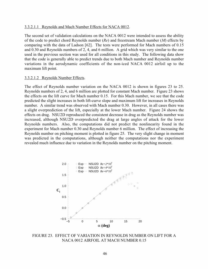
46

3.3.2.1.1 Reynolds and Mach Number Effects for NACA 0012.

The second set of validation calculations on the NACA 0012 were intended to assess the abilityof the code to predict chord Reynolds number (Re) and freestream Mach number (M) effects bycomparing with the data of Ladson [62]. The tests were performed for Mach numbers of 0.15and 0.30 and Reynolds numbers of 2, 4, and 6 million. A grid which was very similar to the oneused in the previous section was used for all conditions in this study. The following data showthat the code is generally able to predict trends due to both Mach number and Reynolds numbervariations in the aerodynamic coefficients of the non-iced NACA 0012 airfoil up to themaximum lift point.

3.3.2.1.2 Reynolds Number Effects.

The effect of Reynolds number variation on the NACA 0012 is shown in figures 23 to 25.Reynolds numbers of 2, 4, and 6 million are plotted for constant Mach number. Figure 23 showsthe effects on the lift curve for Mach number 0.15. For this Mach number, we see that the codepredicted the slight increases in both lift-curve slope and maximum lift for increases in Reynoldsnumber. A similar trend was observed with Mach number 0.30. However, in all cases there wasa slight overprediction of the lift, especially at the lower Mach number. Figure 24 shows theeffects on drag. NSU2D reproduced the consistent decrease in drag as the Reynolds number wasincreased, although NSU2D overpredicted the drag at large angles of attack for the lowerReynolds numbers. Also, the computations did not predict the nonlinearity found in theexperiment for Mach number 0.30 and Reynolds number 6 million. The effect of increasing theReynolds number on pitching moment is plotted in figure 25. The very slight change in momentwas predicted in the computations, although neither the computations nor the experimentrevealed much influence due to variation in the Reynolds number on the pitching moment.

−5 0 5 10 15 20

α (deg)

−0.5

0.0

0.5

1.0

1.5

2.0

Cl

ExpExpExp

NSU2D Re=2*106

NSU2D Re=4*106

NSU2D Re=6*106

FIGURE 23. EFFECT OF VARIATION IN REYNOLDS NUMBER ON LIFT FOR ANACA 0012 AIRFOIL AT MACH NUMBER 0.15

47

0.00 0.01 0.02 0.03 0.04 0.05

Cd

−0.5

0.0

0.5

1.0

1.5

2.0

Cl

ExpExpExp

NSU2D Re=2*106

NSU2D Re=4*106

NSU2D Re=6*106

FIGURE 24. EFFECT OF VARIATION IN REYNOLDS NUMBER ON DRAG FOR ANACA 0012 AIRFOIL AT MACH NUMBER 0.15

−5 0 5 10 15 20

α (deg)

−0.2

−0.1

0.0

0.1

0.2

Cm

ExpExpExp

NSU2D Re=2*106

NSU2D Re=4*106

NSU2D Re=6*106

FIGURE 25. EFFECT OF VARIATION IN REYNOLDS NUMBER ON PITCHINGMOMENT FOR A NACA 0012 AIRFOIL AT MACH NUMBER 0.15

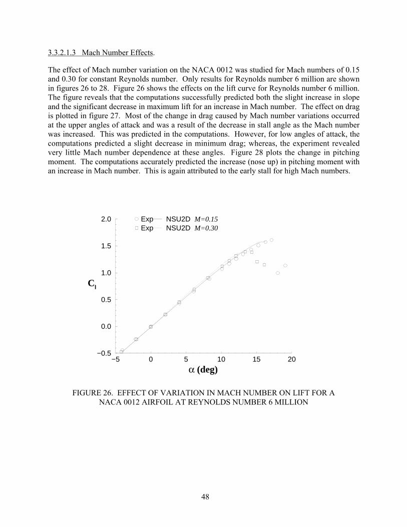
48

3.3.2.1.3 Mach Number Effects.

The effect of Mach number variation on the NACA 0012 was studied for Mach numbers of 0.15and 0.30 for constant Reynolds number. Only results for Reynolds number 6 million are shownin figures 26 to 28. Figure 26 shows the effects on the lift curve for Reynolds number 6 million.The figure reveals that the computations successfully predicted both the slight increase in slopeand the significant decrease in maximum lift for an increase in Mach number. The effect on dragis plotted in figure 27. Most of the change in drag caused by Mach number variations occurredat the upper angles of attack and was a result of the decrease in stall angle as the Mach numberwas increased. This was predicted in the computations. However, for low angles of attack, thecomputations predicted a slight decrease in minimum drag; whereas, the experiment revealedvery little Mach number dependence at these angles. Figure 28 plots the change in pitchingmoment. The computations accurately predicted the increase (nose up) in pitching moment withan increase in Mach number. This is again attributed to the early stall for high Mach numbers.

−5 0 5 10 15 20

α (deg)

−0.5

0.0

0.5

1.0

1.5

2.0

Cl

ExpExp

NSU2D M=0.15NSU2D M=0.30

FIGURE 26. EFFECT OF VARIATION IN MACH NUMBER ON LIFT FOR ANACA 0012 AIRFOIL AT REYNOLDS NUMBER 6 MILLION

49

0.00 0.01 0.02 0.03 0.04 0.05

Cd

−0.5

0.0

0.5

1.0

1.5

2.0

Cl

ExpExp


FIGURE 27. EFFECT OF VARIATION IN MACH NUMBER ON DRAG FOR ANACA 0012 AIRFOIL AT REYNOLDS NUMBER 6 MILLION

−5 0 5 10 15 20

α (deg)

−0.2

−0.1

0.0

0.1

0.2

Cm

ExpExp


FIGURE 28. EFFECT OF VARIATION IN MACH NUMBER ON PITCHING MOMENTFOR A NACA 0012 AIRFOIL AT REYNOLDS NUMBER 6 MILLION

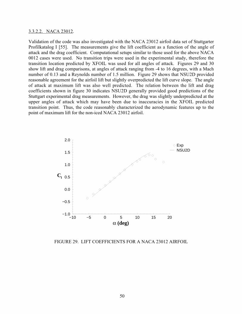
50

3.3.2.2. NACA 23012.

Validation of the code was also investigated with the NACA 23012 airfoil data set of StuttgarterProfilkatalog I [55]. The measurements give the lift coefficient as a function of the angle ofattack and the drag coefficient. Computational setups similar to those used for the above NACA0012 cases were used. No transition trips were used in the experimental study, therefore thetransition location predicted by XFOIL was used for all angles of attack. Figures 29 and 30show lift and drag comparisons, at angles of attack ranging from -4 to 16 degrees, with a Machnumber of 0.13 and a Reynolds number of 1.5 million. Figure 29 shows that NSU2D providedreasonable agreement for the airfoil lift but slightly overpredicted the lift curve slope. The angleof attack at maximum lift was also well predicted. The relation between the lift and dragcoefficients shown in figure 30 indicates NSU2D generally provided good predictions of theStuttgart experimental drag measurements. However, the drag was slightly underpredicted at theupper angles of attack which may have been due to inaccuracies in the XFOIL predictedtransition point. Thus, the code reasonably characterized the aerodynamic features up to thepoint of maximum lift for the non-iced NACA 23012 airfoil.

−10 −5 0 5 10 15 20

α (deg)

−1.0

−0.5

0.0

0.5

1.0

1.5

2.0

Cl

ExpNSU2D

FIGURE 29. LIFT COEFFICIENTS FOR A NACA 23012 AIRFOIL

51

0.00 0.05 0.10

Cd

−1.0

−0.5

0.0

0.5

1.0

1.5

2.0

Cl

ExpNSU2D

FIGURE 30. DRAG COEFFICIENTS FOR A NACA 23012 AIRFOIL

3.3.2.3 NACA 23012m With an Undeflected Flap.

The primary airfoil for the icing investigation was a modified version of the NACA 23012 with a25 % chord simple flap. Therefore, simulations of the clean configuration (with boundary layertrip) for this model will be tested first. The NACA 23012 airfoil was chosen because it hasaerodynamic characteristics that are typical of the current commuter aircraft fleet. Along withthe addition of the simple flap, the actual airfoil tested had a few modifications from the standardNACA 23012. Refer to section 3.1 for the detailed explanation of the modifications to NACA23012. Due to the variations, this model will be referred to as the NACA 23012m airfoil.

The predictions obtained from NSU2D are compared with the experimental data of Lee andBragg [29]. The data were collected for a Mach number of 0.2 and a Reynolds number of1.8 × 106 with transition trips placed at the 2% chord location on the upper surface and 5% on thelower surface. The experimental data have been corrected for wall interference.

Due to the added complexity of the flap element, the computational domain required slightlyincreased grid resolution. For these simulations, the computational domain was a square region,50 × 50 chords, with the airfoil in the center. This domain is shown in figure 31. Far fieldboundary conditions were used on the outer boundary. The high-resolution grid containedapproximately 70,000 nodes with 900 points distributed along the surface of the two elements.In the direction normal to the airfoil surface, the first node was located at approximately a y/c of2 × 10-6 with a 15% successive increase in grid size away from the wall.

52

FIGURE 31. MESH FOR NACA 23012m, (a) FAR FIELD, (b) CLOSEUP, AND (c) FLAP

(c)

(b)

(a)

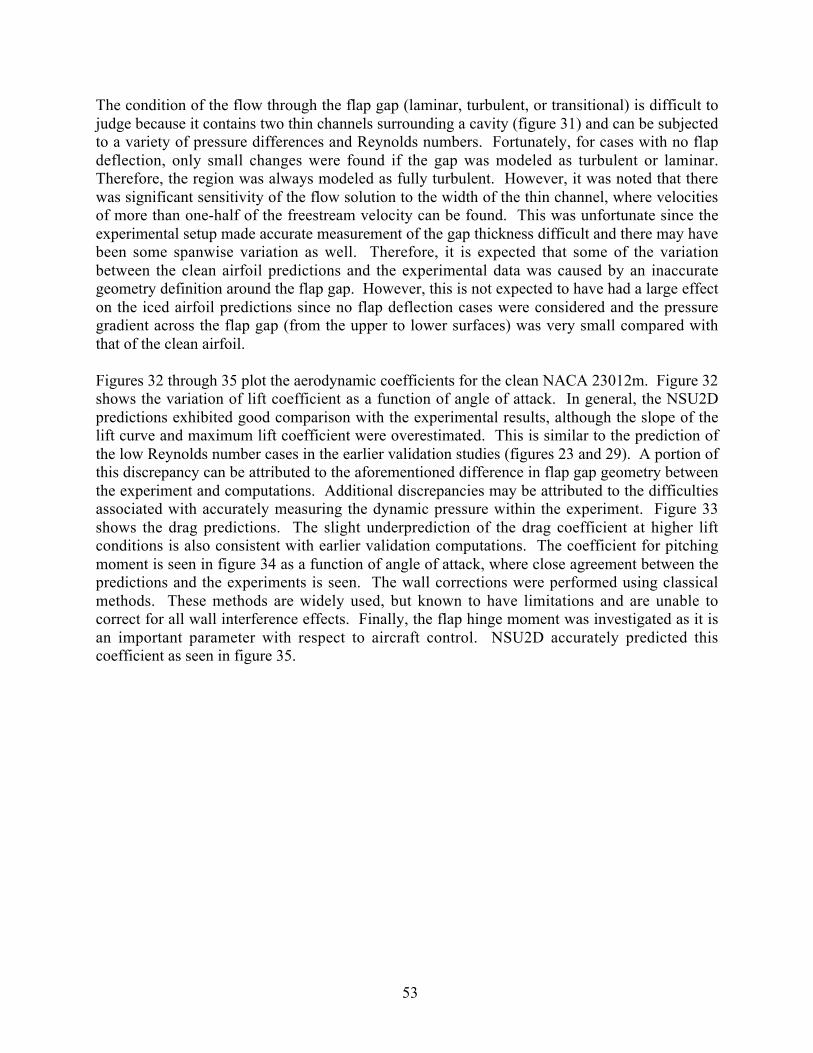
53

The condition of the flow through the flap gap (laminar, turbulent, or transitional) is difficult tojudge because it contains two thin channels surrounding a cavity (figure 31) and can be subjectedto a variety of pressure differences and Reynolds numbers. Fortunately, for cases with no flapdeflection, only small changes were found if the gap was modeled as turbulent or laminar.Therefore, the region was always modeled as fully turbulent. However, it was noted that therewas significant sensitivity of the flow solution to the width of the thin channel, where velocitiesof more than one-half of the freestream velocity can be found. This was unfortunate since theexperimental setup made accurate measurement of the gap thickness difficult and there may havebeen some spanwise variation as well. Therefore, it is expected that some of the variationbetween the clean airfoil predictions and the experimental data was caused by an inaccurategeometry definition around the flap gap. However, this is not expected to have had a large effecton the iced airfoil predictions since no flap deflection cases were considered and the pressuregradient across the flap gap (from the upper to lower surfaces) was very small compared withthat of the clean airfoil.

Figures 32 through 35 plot the aerodynamic coefficients for the clean NACA 23012m. Figure 32shows the variation of lift coefficient as a function of angle of attack. In general, the NSU2Dpredictions exhibited good comparison with the experimental results, although the slope of thelift curve and maximum lift coefficient were overestimated. This is similar to the prediction ofthe low Reynolds number cases in the earlier validation studies (figures 23 and 29). A portion ofthis discrepancy can be attributed to the aforementioned difference in flap gap geometry betweenthe experiment and computations. Additional discrepancies may be attributed to the difficultiesassociated with accurately measuring the dynamic pressure within the experiment. Figure 33shows the drag predictions. The slight underprediction of the drag coefficient at higher liftconditions is also consistent with earlier validation computations. The coefficient for pitchingmoment is seen in figure 34 as a function of angle of attack, where close agreement between thepredictions and the experiments is seen. The wall corrections were performed using classicalmethods. These methods are widely used, but known to have limitations and are unable tocorrect for all wall interference effects. Finally, the flap hinge moment was investigated as it isan important parameter with respect to aircraft control. NSU2D accurately predicted thiscoefficient as seen in figure 35.

54

−20 −15 −10 −5 0 5 10 15 20

α (deg)

−1.0

−0.5

0.0

0.5

1.0

1.5

2.0

Cl

ExpNSU2D

FIGURE 32. LIFT COEFFICIENTS FOR A NACA 23012m AIRFOIL

0.00 0.05 0.10 0.15 0.20 0.25

Cd

−1.0

−0.5

0.0

0.5

1.0

1.5

2.0

Cl

ExpNSU2D

FIGURE 33. DRAG COEFFICIENTS FOR A NACA 23012m AIRFOIL

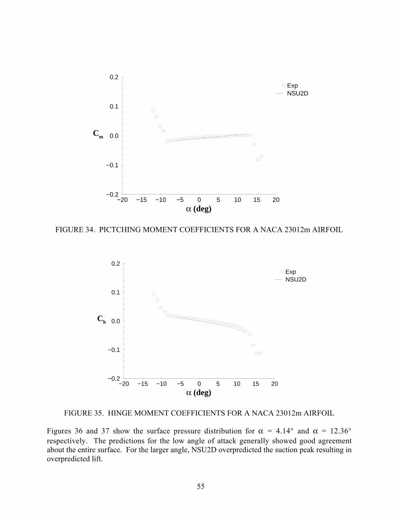
55

−20 −15 −10 −5 0 5 10 15 20

α (deg)

−0.2

−0.1

0.0

0.1

0.2

Cm

ExpNSU2D

FIGURE 34. PICTCHING MOMENT COEFFICIENTS FOR A NACA 23012m AIRFOIL

−20 −15 −10 −5 0 5 10 15 20

α (deg)

−0.2

−0.1

0.0

0.1

0.2

Ch

ExpNSU2D

FIGURE 35. HINGE MOMENT COEFFICIENTS FOR A NACA 23012m AIRFOIL

Figures 36 and 37 show the surface pressure distribution for α = 4.14° and α = 12.36°respectively. The predictions for the low angle of attack generally showed good agreementabout the entire surface. For the larger angle, NSU2D overpredicted the suction peak resulting inoverpredicted lift.

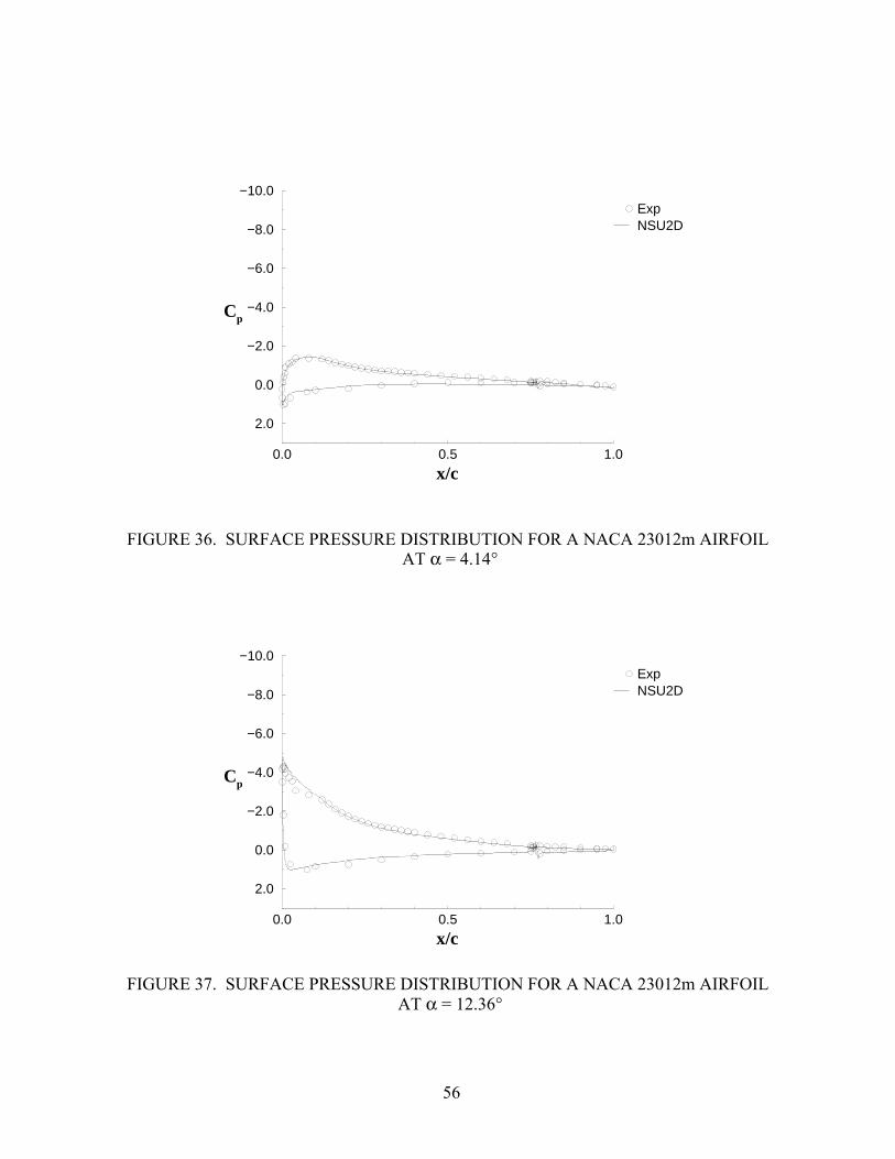
56

0.0 0.5 1.0

x/c

−10.0

−8.0

−6.0

−4.0

−2.0

0.0

2.0

Cp

ExpNSU2D

FIGURE 36. SURFACE PRESSURE DISTRIBUTION FOR A NACA 23012m AIRFOIL AT α = 4.14°

0.0 0.5 1.0

x/c

−10.0

−8.0

−6.0

−4.0

−2.0

0.0

2.0

Cp

ExpNSU2D

FIGURE 37. SURFACE PRESSURE DISTRIBUTION FOR A NACA 23012m AIRFOIL AT α = 12.36°

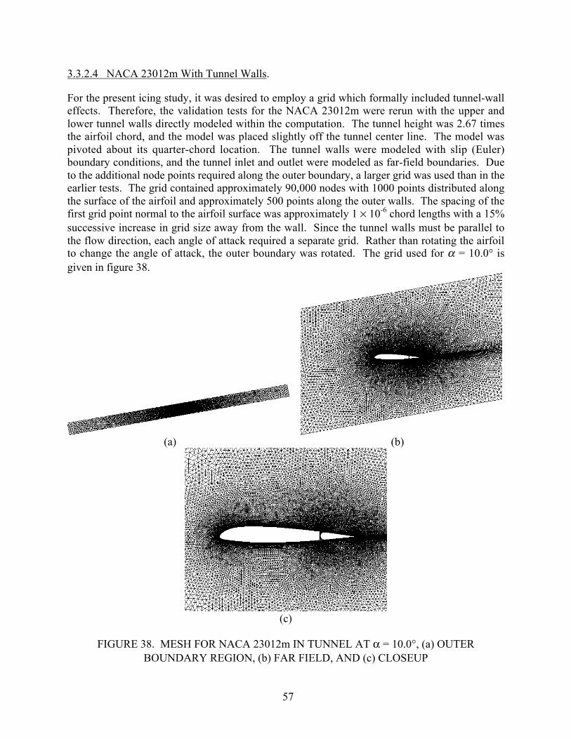
57

3.3.2.4 NACA 23012m With Tunnel Walls.

For the present icing study, it was desired to employ a grid which formally included tunnel-walleffects. Therefore, the validation tests for the NACA 23012m were rerun with the upper andlower tunnel walls directly modeled within the computation. The tunnel height was 2.67 timesthe airfoil chord, and the model was placed slightly off the tunnel center line. The model waspivoted about its quarter-chord location. The tunnel walls were modeled with slip (Euler)boundary conditions, and the tunnel inlet and outlet were modeled as far-field boundaries. Dueto the additional node points required along the outer boundary, a larger grid was used than in theearlier tests. The grid contained approximately 90,000 nodes with 1000 points distributed alongthe surface of the airfoil and approximately 500 points along the outer walls. The spacing of thefirst grid point normal to the airfoil surface was approximately 1 × 10-6 chord lengths with a 15%successive increase in grid size away from the wall. Since the tunnel walls must be parallel tothe flow direction, each angle of attack required a separate grid. Rather than rotating the airfoilto change the angle of attack, the outer boundary was rotated. The grid used for α = 10.0° isgiven in figure 38.

(a) (b)

(c)

FIGURE 38. MESH FOR NACA 23012m IN TUNNEL AT α = 10.0°, (a) OUTERBOUNDARY REGION, (b) FAR FIELD, AND (c) CLOSEUP

58

To verify this approach for NSU2D, the earlier simulations using free boundary conditions in thefar field were compared with simulations where the tunnel walls were modeled directly. Theaerodynamic coefficients computed in the simulations with tunnel walls were theoreticallycorrected a posteriori to an infinite domain using the theory of Rae and Pope [36]. Thesecomparisons are found in figures 39 through 42. There was very little variation between theresults obtained from the two simulation methods for lift (figure 39) and drag (figure 40), in factthe curves are barely distinguishable. However, the pitching moment (figure 41) did not have asgood agreement. Simulating the tunnel walls predicted a curve which was much more flat thanthe computations without walls. It is assumed that this variation is caused in part by theinaccurate assumptions associated with using linear theory to determine the influence of tunnelwalls. The two methods provided decent agreement for the hinge moment (figure 42), althoughthe theoretical correction suffers from the same inadequacies as the pitching moment correction.Therefore, it is felt to be important to model tunnel walls directly when investigatingaerodynamic moments.

−20 −15 −10 −5 0 5 10 15 20

α (deg)

−1.0

−0.5

0.0

0.5

1.0

1.5

2.0

Cl

Far−FieldEuler Walls

FIGURE 39. LIFT COEFFICIENTS FOR A NACA 23012m AIRFOIL MODELED FOR TWOMETHODS (1) EULER-WALLS WHERE THE TUNNEL WALLS (AND CORRECTED

USING THE THEORY OF RAE AND POPE) AND (2) FAR FIELD WHERE THE AIRFOILWAS SIMULATED WITHOUT TUNNEL WALLS

59

0.00 0.05 0.10 0.15 0.20 0.25

Cd

−1.0

−0.5

0.0

0.5

1.0

1.5

2.0

Cl


FIGURE 40. DRAG COEFFICIENTS FOR A NACA 23012m AIRFOIL MODELED WITHTUNNEL WALLS WERE SIMULATED DIRECTLY AND SUBSEQUENTLY CORRECTED

USING THE THEORY OF RAE AND POPE TO FREE FLIGHT CONDITIONS AND FARFIELD WHERE THE AIRFOIL WAS SIMULATED WITHOUT TUNNEL WALLS

−20 −15 −10 −5 0 5 10 15 20

α (deg)

−0.2

−0.1

0.0

0.1

0.2

Cm


FIGURE 41. PITCHING MOMENT COEFFICIENTS FOR A NACA 23012m AIRFOILMODELED WITH TUNNEL WALLS (AND CORRECTED USING THE THEORY OF RAE

AND POPE) AND WITHOUT TUNNEL WALLS

60

−20 −15 −10 −5 0 5 10 15 20

α (deg)

−0.2

−0.1

0.0

0.1

0.2

Ch


FIGURE 42. HINGE MOMENT COEFFICIENTS FOR A NACA 23012m AIRFOILMODELED WITH TUNNEL WALLS (AND CORRECTED USING THE THEORY OF RAE

AND POPE) AND WITHOUT TUNNEL WALLS

3.3.2.5 NLF 0414 Simulations.

The predictions obtained from NSU2D are compared with the experimental data of Lee andBragg [29]. The data were collected for a Mach number of 0.2 and a Reynolds number of1.8 × 106 with transition trips placed at the 2% chord location on the upper surface and 5% chordlocation on the lower surface. The experimental data has been corrected for wall interference.The simulations were carried out for the tunnel case with the same transition point specificationtechnique used for the other airfoils.

Figures 43 through 46 plot the aerodynamic coefficients for the clean NLF 0414. Figure 43shows the variation of lift coefficient as a function of angle of attack. The slope of the lift curveand maximum lift coefficient were overestimated by the computations. In fact, there are nocomparisons of CFD solutions with experimental lift and pressure distributions in the openliterature. It is well known that the flow field for this airfoil is difficult to predict with CFDtechniques at these low Reynolds numbers. The differences are attributed to large regions oftransitional flow (neither laminar nor turbulent) which the present methodology cannot predict.When simulations were run without the tunnel walls, there was a small improvement in the forceand moment curves, but this approach was not used because of a desire to be consistent with allcases. Figure 44 shows the drag predictions. The slight underprediction of the drag coefficientat higher lift conditions is also consistent with earlier validation computations. The coefficientfor pitching moment is seen in figure 45 as a function of angle of attack, where better agreementbetween the predictions and the experiments is seen. The flap hinge moment was investigated as

61

it is an important parameter with respect to aircraft control. NSU2D predicted this coefficientreasonably well as seen in figure 46.

−20 −15 −10 −5 0 5 10 15 20

α (deg)

−1.0

−0.5

0.0

0.5

1.0

1.5

2.0

Cl

ExpNSU2D

FIGURE 43. LIFT COEFFICIENTS FOR A NLF 0414 AIRFOIL MODELED WITH TUNNEL WALLS

0.00 0.05 0.10 0.15 0.20 0.25

Cd

−1.0

−0.5

0.0

0.5

1.0

1.5

2.0

Cl

ExpNSU2D

FIGURE 44. DRAG COEFFICIENTS FOR A NLF 0414 AIRFOIL MODELED WITH TUNNEL WALLS

62

−20 −15 −10 −5 0 5 10 15 20

α (deg)

−0.2

−0.1

0.0

0.1

0.2

Cm

ExpNSU2D

FIGURE 45. PITCHING MOMENT COEFFICIENTS FOR A NLF 0414 AIRFOILMODELED WITH TUNNEL WALLS

−20 −15 −10 −5 0 5 10 15 20

α (deg)

−0.3

−0.2

−0.1

0.0

0.1

0.2

Ch

ExpNSU2D

FIGURE 46. HINGE MOMENT COEFFICIENTS FOR A NLF 0414 AIRFOILMODELED WITH TUNNEL WALLS

63

Figure 47 shows the surface pressure distributions for α = 6°, α = 0°, and α = 10°. It isinteresting to note that the disagreement with experimental pressure distribution is small,considering the comparison of lift coefficients at these angles. The main differences in thepressure distribution occur in the pressure recovery region and some differences exist on thelower surface.

In conclusion, NSU2D has been validated for basic fluid dynamic features associated with aniced airfoil: laminar and turbulent boundary layer flow, backward-facing step, and threemarkedly different clean airfoil shapes.

3.3.3 Iced Airfoil SimulationsNACA 0012 With Glaze Ice.

For further code validation, a leading-edge glaze ice shape on a NACA 0012 airfoil wasconsidered. Although, the primary objective for this research was to simulate large-droplet iceaccretion shapes, this shape provides a good comparison with the more commonly studied iceshape aerodynamics. This ice shape can be seen in the mesh shown in figure 48. The gridcontained about 60,000 nodes and used far field conditions at the outer boundary. Theexperimental data of Bragg [63] was used for comparison. As described in the experimental dataset, these runs probably did not have large regions of laminar flow due to the large and complexice shape and therefore turbulence was modeled over the entire airfoil surface. Potapczuk [64]found that although modeling laminar regions around the ice shape influenced the velocityprofiles along the airfoil surface, simulating laminar flow did not greatly influence the integratedaerodynamic forces. Therefore, modeling the entire surface as turbulent seems reasonable andappropriate. All runs were made at a Mach number of 0.12 and a Reynolds number of 1.5 × 106.

Figures 49 through 51 show aerodynamic predictions for angles of attack from -6 to +6 degrees.These predictions indicate that NSU2D was able to reasonably evaluate performancecharacteristics for an iced airfoil with large separation regions at low angles of attack.Calculations for -8 and +8 degrees failed to converge, which is attributed to inherentunsteadiness in the flow due to the presence of vortex shedding off the horns of the ice shape.The computed values for the lift coefficient (figure 49) agreed reasonably well with theexperiments, although the lift curve slope was slightly underpredicted. This was a result of amore rapid predicted pressure recovery within the separated regions than was measured in theexperiment. The drag (figure 50) and moment (figure 51) were also very well predicted,considering the large amount of separation on the airfoil.

64

0.0 0.5 1.0

x/c

−10.0

−8.0

−6.0

−4.0

−2.0

0.0

2.0

Cp

ExpNSU2D

(a)

0.0 0.5 1.0

x/c

−10.0

−8.0

−6.0

−4.0

−2.0

0.0

2.0

Cp

ExpNSU2D

(b)

0.0 0.5 1.0

x/c

−10.0

−8.0

−6.0

−4.0

−2.0

0.0

2.0

Cp

ExpNSU2D

(c)

FIGURE 47. SURFACE PRESSURE DISTRIBUTION FOR A NLF 0414 AIRFOIL AT (a) α = -6°, (b) α = 0°, AND (c) α = 10°

65

(a)

(b)

(c)FIGURE 48. MESH FOR NACA 0012M (a) FAR FIELD WHERE AIRFOIL IS INSIDE THE

CLUSTERED GRIDS, (b) CLOSEUP OF AIRFOIL, AND (c) CLOSEUP OF ICE SHAPE

66

−10 −5 0 5 10

α (deg)

−1.0

−0.5

0.0

0.5

1.0

Cl

ExpNSU2D

FIGURE 49. LIFT COEFFICIENTS FOR A NACA 0012m AIRFOIL WITHLEADING-EDGE GLAZE ICE

0.00 0.05 0.10

Cd

−1.0

−0.5

0.0

0.5

1.0

Cl

ExpNSU2D

FIGURE 50. DRAG COEFFICIENTS FOR A NACA 0012m AIRFOIL WITHLEADING-EDGE GLAZE ICE

67

−10 −5 0 5 10

α (deg)

−0.4

−0.3

−0.2

−0.1

0.0

0.1

0.2

0.3

0.4

Cm

ExpNSU2D

FIGURE 51. MOMENT COEFFICIENTS FOR A NACA 0012m AIRFOIL WITHLEADING-EDGE GLAZE ICE

Figure 52 shows the surface pressure distribution for α = 4.12°. This figure shows goodagreement in the attached regions of the flow, but the plot shows a faster pressure recoverywithin the separated regions on both the upper and lower surfaces. This is especially noticeableon the upper surface. The plots also reveal a small pressure spike/discontinuity on the lowersurface ice horn. This maybe an indication of insufficient grid resolution within this region or aresult of the surface slope discontinuity. The pressure distributions for this geometry at otherangles of attack showed similar agreement.

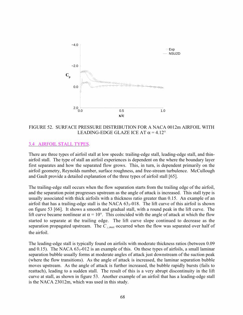
68

0.0 0.5 1.0

x/c

−4.0

−2.0

0.0

2.0

Cp

ExpNSU2D

FIGURE 52. SURFACE PRESSURE DISTRIBUTION FOR A NACA 0012m AIRFOIL WITHLEADING-EDGE GLAZE ICE AT α = 4.12°

3.4 AIRFOIL STALL TYPES.

There are three types of airfoil stall at low speeds: trailing-edge stall, leading-edge stall, and thin-airfoil stall. The type of stall an airfoil experiences is dependent on the where the boundary layerfirst separates and how the separated flow grows. This, in turn, is dependent primarily on theairfoil geometry, Reynolds number, surface roughness, and free-stream turbulence. McCulloughand Gault provide a detailed explanation of the three types of airfoil stall [65].

The trailing-edge stall occurs when the flow separation starts from the trailing edge of the airfoil,and the separation point progresses upstream as the angle of attack is increased. This stall type isusually associated with thick airfoils with a thickness ratio greater than 0.15. An example of anairfoil that has a trailing-edge stall is the NACA 633-018. The lift curve of this airfoil is shownon figure 53 [66]. It shows a smooth and gradual stall, with a round peak in the lift curve. Thelift curve became nonlinear at α = 10°. This coincided with the angle of attack at which the flowstarted to separate at the trailing edge. The lift curve slope continued to decrease as theseparation propagated upstream. The C l ,max occurred when the flow was separated over half ofthe airfoil.

The leading-edge stall is typically found on airfoils with moderate thickness ratios (between 0.09and 0.15). The NACA 633-012 is an example of this. On these types of airfoils, a small laminarseparation bubble usually forms at moderate angles of attack just downstream of the suction peak(where the flow transitions). As the angle of attack is increased, the laminar separation bubblemoves upstream. As the angle of attack is further increased, the bubble rapidly bursts (fails toreattach), leading to a sudden stall. The result of this is a very abrupt discontinuity in the liftcurve at stall, as shown in figure 53. Another example of an airfoil that has a leading-edge stallis the NACA 23012m, which was used in this study.

69

The thin-airfoil stall occurs on all sharp-edge airfoils and some thin airfoils (with a thicknessratio less than 0.09). The double-wedge airfoil shown on figure 53 is an example of this. Thethin-airfoil stall is characterized by a flow separation that forms on the leading edge of the airfoilthat grows downstream with increasing angle of attack. This growth in the separation bubble ismuch more gradual than the sudden bubble burst that occurs on the leading-edge stall, resultingin a much more gradual stall. A “kink” in the lift curve is often observed when the leading-edgebubble starts to grow rapidly. On the double-wedge airfoil, this occurs at α = 2°. The liftreaches a maximum when the bubble fails to reattach. The top of the curve is relatively flat withlittle lift loss after stall.

An airfoil can also have stall characteristics that are a combination of two of the types describedabove. An example of this is the combination of the thin-airfoil and the trailing-edge stall. Flowseparation can form both at the leading and the trailing edge. As the angle of attack is increased,the separation will grow until the two bubbles join near stall.

0

5

10

15

0 5 10 15 20

NACA 633-018: Trailing Edge

NACA 633-012: Leading Edge

Double Wedge: Thin Airfoil

Cl

α (°)

FIGURE 53. LIFT CHARACTERISTICS OF THE THREE AIRFOIL STALL TYPES

4. RESULTS AND DISCUSSION.

4.1 EXPERIMENTAL RESULTS.

The C l and Cm data in this section come from the integrated surface pressures and the Cd

measurements were taken from the wake pressure data unless otherwise indicated. The Ch datawere taken from the flap hinge balance measurements.

70

4.1.1 Effect of Simulated Ice Ridge Location.

Figure 54 shows the effect of the 0.25″ (k/c = 0.0139) forward-facing quarter-round icesimulation at three different x/c locations on the aerodynamic coefficients. The boundary layerwas tripped (at 2% chord upper and 5% lower surface) for the cases with the simulated iceshapes at x/c = 0.10 and x/c = 0.20. All of the simulated ice cases showed reduced lift curveslopes in the linear regions (-5° < α < 1°) when compared to the clean case (figure 54(a)).Varying the ice shape location from x/c = 0.02 to 0.20 had large effects on the lift of the NACA23012m. The simulated ice cases exhibited gradual stall characteristics typical of a thin-airfoil-type stall and not the leading-edge stall of the clean model. (See discussion of types of airfoilstall in section 3.4.) Of the three cases shown, the loss in lift was most severe when the ice shapewas located at x/c = 0.10 (with Cl,max = 0.27). It will be shown later that the worst ice shape

location for Cl,max degradation was at x/c = 0.12. When the ice shape was located at x/c = 0.02,

Cl,max was approximately doubled. A classical Cl,max (as α is increased Cl eventually reaches a

maximum and then decreases) was not observed when the simulated ice shape was located atx/c = 0.20. Instead, only an inflection in the curve was observed at α = 4° (and Cl = 0.42).

Jacobs [12] observed similar lift curves (where a real Cl,max was not observed) under certain

conditions in his test of protuberances on a NACA 0012 airfoil.

Figure 54(b) shows the drag polars with the 0.25″ simulated ice shape at the three different x/clocations. Figure 54(b) shows significant increases in drag when the simulated ice shape waspresent. The largest increase in drag for Cl > 0 occurred when the simulated ice shape was at x/c

= 0.10, which also corresponds to the case with the lowest Cl . However, at Cl < 0, the largest

increase in drag occurred when the simulated ice shape was located at x/c = 0.20.

The pitching moments with the three simulated ice shape locations are shown in figure 54(c).When the simulated ice shape was at x/c = 0.10 and 0.20, the pitching moment exhibited a largebreak in the slope at l = -1°, becoming more negative, indicating that the airfoil was more aft

loaded. When the simulated ice shape was located at x/c = 0.02, the pitching moment diverged atl = 5°. However, between l = 0° and 5°, the pitching moment was more positive than the clean

case. Figure 54(d) shows the flap hinge moments with the simulated ice shape at the threedifferent x/c locations. Between l = -9° and l = 1°, the hinge moments with a simulated ice

shape present were higher than that of the non-iced case, indicating a larger trailing-edge downmoment about the flap hinge. The cases with the simulated ice shape at x/c = 0.10 and 0.20exhibited a large break in the l slope at l = 0°. The case with the simulated ice shape at

x/c = 0.02 exhibited a large break in the slope l = 6°. Figures 54(c) and 54(d) show that the

sudden divergence in the flap hinge moment occurred at an angle of attack that was a fewdegrees higher than that of the pitching moment.

71

-1

-0.50

0.51

1.52

-15

-10

-50

510

1520

Cle

anx/

c =

0.0

2x/

c =

0.1

0x/

c =

0.2

0

Cl

α (

°)

-1

-0.50

0.51

1.5

00.

050.

10.

15

Cle

anx/

c =

0.0

2x/

c =

0.1

0x/

c =

0.2

0

Cl

Cd

(a)

Lif

t(b

) D

rag

-0.1

-0.0

50

0.050.1

-15

-10

-50

510

1520

Cle

anx/

c =

0.0

2x/

c =

0.1

0x/

c =

0.2

0

Cm

α (

°)

-0.2

5

-0.2

-0.1

5

-0.1

-0.0

50

0.050.

1 -15

-10

-50

510

1520

Cle

anx/

c =

0.0

2x/

c =

0.1

0x/

c =

0.2

0Ch

α (

°)

(c)

Pitc

hing

Mom

ent

(d)

Flap

Hin

ge M

omen

t

FIG

UR

E 5

4. E

FFE

CT

S O

F SI

MU

LA

TE

D I

CE

SH

APE

LO

CA

TIO

N O

N A

ER

OD

YN

AM

IC C

OE

FFIC

IEN

TS

(NA

CA

230

12m

0.2

5˝ f

orw

arde

d-fa

cing

qua

rter

rou

nd, b

ound

ary

laye

r tr

ippe

d fo

r x/c

= 0.

10 a

nd x/c

= 0

.20

case

s, Re

= 1.

8 m

illio

n)

72

Figure 54 shows the summary of Cl,max versus the chordwise location of the simulated ice

accretion (0.25″ forward-facing quarter round) as well as the clean airfoil Cl,max with natural

transition. All of the cases with the simulated ice shapes at, down stream of, 4% chord had theboundary layer tripped at 2% chord upper and 5% chord lower surface. The cases with thesimulated ice shapes upstream of 4% chord were not tripped. The lowest Cl,max for the 0.25˝

shape (k/c = 0.0139) was 0.25 and occurred at x/c = 0.12. The maximum lift increased rapidlyas the simulated ice was moved forward of this location, reaching 0.97 at the leading edge.Thus, it is clear from figure 55 that in terms of maximum lift loss, the most critical location forthis simulated ice shapes was at x/c = 0.12.

0.2

0.4

0.6

0.8

1

1.2

1.4

1.6

0 0.1 0.2 0.3 0.4 0.5

Clean Simulated Ice

Cl,

max

Ice Shape Location (x/c)

FIGURE 55. SUMMARY OF Cl,max WITH SIMULATED ICE SHAPE AT

VARIOUS LOCATIONS(NACA 23012m, forward-facing quarter round, boundary layer tripped

for case with simulated ice at x/c ≥ 0.04, Re = 1.8 million)

As stated in the introduction, studies [12, 13] have shown that the effects of a spanwise surfaceprotuberance (of k/c < 0.005) on lift, drag, and pitching moment became more severe as it wasmoved closer to the leading edge. Gregory and O’Reilly [67] showed that the k/c = 0.0004surface roughness resulted in the most severe loss in Cl,max (on a NACA 0012 airfoil) when it

was placed at the leading edge. Bowden [13] observed that the maximum increase in the dragoccurred when the protuberance was located near the location of maximum local surface velocity(or minimum Cp). A possible explanation for this is that the protuberance would extract thegreatest amount of boundary layer momentum when placed at that location, which would thickenthe boundary layer and increase drag. Figure 56 shows the drag increase (compared to the cleanairfoil) due to the 0.25″ ice shape simulation. Each curve represents a fixed angle of attack, andthe simulated ice shape location is depicted on the x axis. Also shown on the figure, by the solid

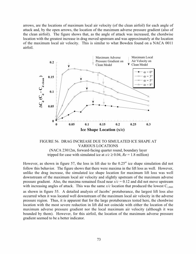
73

arrows, are the locations of maximum local air velocity (of the clean airfoil) for each angle ofattack and, by the open arrows, the location of the maximum adverse pressure gradient (also ofthe clean airfoil). The figure shows that, as the angle of attack was increased, the chordwiselocation with the greatest increase in drag moved upstream and was approximately at the locationof the maximum local air velocity. This is similar to what Bowden found on a NACA 0011airfoil.

0

0.05

0.1

0.15

0.2

0 0.05 0.1 0.15 0.2 0.25 0.3

α = 0°α = 3°α = 5°α = 8°

∆Cd (

Cd -

Cd cl

ean )


Maximum LocalAir Velocity onClean Model

Maximum AdversePressure Gradient onClean Model

FIGURE 56. DRAG INCREASE DUE TO SIMULATED ICE SHAPE ATVARIOUS LOCATIONS

(NACA 23012m, forward-facing quarter round, boundary layertripped for case with simulated ice at x/c ≥ 0.04, Re = 1.8 million)

However, as shown in figure 57, the loss in lift due to the 0.25″ ice shape simulation did notfollow this behavior. The figure shows that there were maxima in the lift loss as well. However,unlike the drag increase, the simulated ice shape location for maximum lift loss was welldownstream of the maximum local air velocity and slightly upstream of the maximum adversepressure gradient. Also, the maxima remained fixed near x/c = 0.12 and did not move upstreamwith increasing angles of attack. This was the same x/c location that produced the lowest Cl,max

as shown in figure 55. A detailed analysis of Jacobs’ protuberance, the largest lift loss alsooccurred when it was located well downstream of the maximum local air velocity in the adversepressure region. Thus, it is apparent that for the large protuberances tested here, the chordwiselocation with the most severe reduction in lift did not coincide with either the location of themaximum adverse pressure gradient nor the local maximum air velocity (although it wasbounded by them). However, for this airfoil, the location of the maximum adverse pressuregradient seemed to be a better indicator.

74

0

0.1

0.2

0.3

0.4

0.5

0.6

0.7

0 0.05 0.1 0.15 0.2 0.25 0.3

α = 0°α = 3°α = 5°α = 8°



Maximum AdversePressure Gradienton Clean Model

∆ Cl(C

l clea

n - C

l )

FIGURE 57. LIFT LOSS DUE TO SIMULATED ICE SHAPE AT VARIOUS LOCATIONS(NACA 23012m, forward-facing quarter round, boundary layer tripped for case with

simulated ice at x/c ≥ 0.04. Re = 1.8 million)

4.1.1.1 Effects of Flap Deflection.

Figure 58 shows the effects of the flap deflection on integrated aerodynamic coefficients. Figure58(a) shows that flap deflection did not significantly alter the lift characteristics of the airfoilwith simulated ice. All three flap deflection cases show a very gradual stall characteristic ofthin-airfoil stall. However, as the flap deflection was increased from -5° to 5°, the angle ofattack at which the lift curve became nonlinear decreased from 3° to 1°. Also, as the flapdeflection was increased, the linear region of the iced cases became increasing shifted verticallyfrom the clean cases (i.e., reduced lift at a given α). At α = -5°, there was almost no verticalshift in the lift curve. However, at α = 5°, there was a 0.08 shift in between the iced and theclean cases.

Figure 58(b) shows the effect of flap deflection on drag. On the clean model, varying the flapdeflection did not change the drag polars by a large amount. However, increasing the flapdeflection did significantly decrease the drag at matched lift coefficients for the case withsimulated ice accretion.

Figures 58(c) and 58(d) show the effect of flap deflection on the pitching and flap hingemoments. Increasing the flap deflection from -5° to 5° did not change where the breaks in theCm curves (with simulated ice shapes) occurred, as it occurred at α = -1° for all three flapdeflections. Varying the flap deflection from -5° to 5° decreased the angle of attack at which theCh curves broke from 2° to 0°. Increasing the flap deflection also increased the differences in Cm

and Ch between the clean and the iced case at negative angles of attack. This was similar to thevertical shift in the linear regions of the lift curve (figure 58(a)).

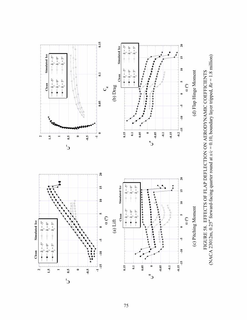
75

-1

-0.50

0.51

1.52 -1

5-1

0-5

05

1015

20

δ f = -

5°

δ f = 0

°

δ f = 5

°

δ f = -

5°

δ f = 0

°

δ f = 5

°

Cl

α (°

)

Cle

anSi

mul

ated

Ice

-1

-0.50

0.51

1.52

00.

050.

10.

15

δ f = -

5°

δ f = 0

°

δ f = 5

°

δ f = -

5°

δ f = 0

°

δ f = 5

°

Cl

Cd

Cle

anSi

mul

ated

Ice

(a)

Lif

t(b

) D

rag

-0.1

5

-0.1

-0.0

50

0.050.1

0.15

-15

-10

-50

510

1520

δ f = -

5°

δ f = 0

°

δ f = 5

°

δ f = -

5°

δ f = 0

°

δ f = 5

°

Cm

α (

°)Cle

anSi

mul

ated

Ice

-0.2

-0.1

5

-0.1

-0.0

50

0.050.1

0.15

-15

-10

-50

510

1520

δ f = -

5°

δ f = 0

°

δ f = 5

°

δ f = -

5°

δ f = 0

°

δ f = 5

°

Ch

α (

°)

Cle

anSi

mul

ated

Ice

(c)

Pitc

hing

Mom

ent

(d)

Flap

Hin

ge M

omen

t

FIG

UR

E 5

8. E

FFE

CT

S O

F FL

AP

DE

FLE

CT

ION

ON

AE

RO

DY

NA

MIC

CO

EFF

ICIE

NT

S(N

AC

A 2

3012

m, 0

.25″

for

war

d-fa

cing

qua

rter

rou

nd a

t x/c

= 0

.10,

bou

ndar

y la

yer

trip

ped,

Re

= 1.

8 m

illio

n)

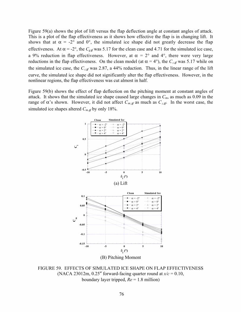
76

Figure 59(a) shows the plot of lift versus the flap deflection angle at constant angles of attack.This is a plot of the flap effectiveness as it shows how effective the flap is in changing lift. Itshows that at α = -2° and 0°, the simulated ice shape did not greatly decrease the flap

effectiveness. At α = -2°, the Cl,δf was 5.17 for the clean case and 4.71 for the simulated ice case,a 9% reduction in flap effectiveness. However, at α = 2° and 4°, there were very largereductions in the flap effectiveness. On the clean model (at α = 4°), the Cl,δf was 5.17 while on

the simulated ice case, the Cl,δf was 2.87, a 44% reduction. Thus, in the linear range of the lift

curve, the simulated ice shape did not significantly alter the flap effectiveness. However, in thenonlinear regions, the flap effectiveness was cut almost in half.

Figure 59(b) shows the effect of flap deflection on the pitching moment at constant angles ofattack. It shows that the simulated ice shape caused large changes in Cm, as much as 0.09 in therange of α’s shown. However, it did not affect Cm,δf as much as Cl,δf. In the worst case, the

simulated ice shapes altered Cm,δf by only 18%.

-0.5

0

0.5

1

-10 -5 0 5 10

α = -2°α = 0°α = 2°α = 4°

α = -2°α = 0°α = 2°α = 4°

Cl

δf (°)

Clean Simulated Ice

(a) Lift

-0.15

-0.1

-0.05

0

0.05

0.1

-10 -5 0 5 10

α = -2°α = 0°α = 2°α = 4°

α = -2°α = 0°α = 2°α = 4°

Cm

δf (°)

Clean Simulated Ice

(B) Pitching Moment

FIGURE 59. EFFECTS OF SIMULATED ICE SHAPE ON FLAP EFFECTIVENESS(NACA 23012m, 0.25″ forward-facing quarter round at x/c = 0.10,

boundary layer tripped, Re = 1.8 million)

77

4.1.1.2 Flow Field Analysis.

The flow field will be discussed next in order to provide a better understanding of the integratedresults shown in the preceding section. Figure 60 summarizes the boundary layer state observedon the model using fluorescent oil flow visualization. The figure shows the progression of theseparation bubbles upstream and downstream of the ice shape simulation as the angle of attackwas increased. Here, the 0.25″ quarter-round ice simulation was located at x/c = 0.10 and theboundary layer was not tripped. The primary separation bubble upstream of the simulated iceshape formed at x/c = 0.07 at α = 0°. The separation point moved gradually upstream tox/c = 0.05 at α = 3° and remained at this location to α = 5°. Evidence of a secondary separationbubble upstream of the simulated ice shape was observed but was not shown because it could notbe accurately measured. The primary downstream bubble reattachment region was locatedbetween x/c = 0.40 and x/c = 0.44 at α = 0°. It was not clearly defined because the reattachmentof the ice-induced bubble was seen in the oil flow as a band of relatively stagnant oil on thesurface. The stagnant oil band was probably an indication of an unsteady reattachment process.The region moved downstream as α was increased and at α = 3.25° was located betweenx/c = 0.75 and the trailing edge. Thus, for the 0.25″ quarter round at x/c = 0.10, the stall wasinitiated by a rapidly growing separation bubble that eventually reached the trailing edge, whichis characteristic of a thin-airfoil stall. Clearly, the separation bubble that formed downstream ofthe simulated ice shape was the most dominant feature in the flow field.

0 0.2 0.4 0.6 0.8 10

1

2

3

4

5

X/C

α (

°)

Ice Shape

Reattachment

Laminar

Forward Bubble

Aft Bubble

Turbulent

FIGURE 60. SUMMARY OF BOUNDARY LAYER STATE WITH THESIMULATED ICE AT x/c = 0.10

(NACA 23012m, forward-facing quarter round, boundary layer not tripped, Re = 1.8 million)

Figure 61 shows the reattachment locations of the separation bubble with the simulated iceshapes at three chordwise locations. Again, this was obtained from flow visualization. Tworeattachment location lines are shown for each of the cases because the reattachment locationwas not clearly defined for large bubbles. Figure 61 shows that when the simulated ice shapewas located at x/c = 0.02, the bubble failed to reattach at α = 7°. When the simulated ice waslocated at x/c = 0.10 and 0.20, the bubble failed to reattach at α = 2.5° and 3°, nearly the sameangle of attack.

x/c

78

-2

0

2

4

6

8

10

0 0.2 0.4 0.6 0.8 1

x/c = 0.02x/c = 0.10x/c = 0.20

α (

°)

xr/c

FIGURE 61. REATTACHMENT LOCATION OF SEPARATION BUBBLE THATFORMED DOWNSTREAM OF SIMULATED ICE

(NACA 23012m, forward-facing quarter round, boundary layer tripped for x/c = 0.10 AND x/c = 0.20 CASES, Re = 1.8 million)

The large change in the flow field around the airfoil can be seen in the pressure distribution plotsof figure 62. Figure 62(a) shows the surface pressure distribution with the 0.25″ ice shapesimulation placed at various chordwise locations at α = 0° and compared to the clean case. Theclean case shows the stagnation point at the leading edge with a suction peak at x/c = 0.12 on theupper surface and at x/c = 0.02 on the lower surface.

The pressure distributions with the simulated ice shape show a severely altered flow field, evenat this angle of attack. It is first important to note that the surface pressure was not measuredover the simulated ice shape. Thus, the Cp from the last pressure tap upstream of the simulatedice shape is connected in the figure to the first pressure tap downstream of the simulated iceshape by a straight line. The flow field became significantly altered when the simulated iceshape was at x/c = 0.02. There was a large suction peak (Cp = -1.16) immediately downstream ofthe simulated ice shape as the flow accelerated over it and separated. However, the simulated iceshape was located in a very favorable pressure gradient and the bubble was able to reattachquickly at x/c = 0.12 (as indicated by figure 61). This allowed another suction peak (dueprimarily to the airfoil geometry and not the simulated ice shape) to form at x/c = 0.18 with aCp value of -0.51.

When the simulated ice shape was located at x/c = 0.10, the flow on the upper surface initiallyaccelerated from the leading-edge stagnation point. However, the flow started to decelerate as itapproached the simulated ice shape and experienced an adverse pressure gradient and flowseparation. This resulted in a local Cp,min of 0.52 located ahead of the simulated ice shape atx/c = 0.03, followed by a local Cp,max of 0.58 at x/c = 0.04. Immediately downstream of thesimulated ice shape, a longer separation bubble was formed, and the Cp was nearly constant at

79

-0.90 until x/c = 0.27, where it started to increase as the reattachment process began. Nearx/c = 0.60, the Cp approached the clean model value and indicated that the flow had reattached.Although the simulated ice shape was located in a favorable pressure gradient, it was so close tothe location of the onset of adverse pressure gradient that the separation bubble was forced toreattach in an adverse pressure gradient. Thus, the separation bubble for this simulated ice shapelocation was much larger than when the simulated ice shape was located at x/c = 0.02.

With the simulated ice shape located at x/c = 0.20, the local Cp,min and Cp,max upstream of thesimulated ice shape became more clearly defined as there was a greater surface length along themodel for the flow to first accelerate and decelerate upstream of the simulated ice shape. In thiscase, the simulated ice shape was located in an adverse pressure gradient and resulted in a verylarge separation bubble that did not reattach until near x/c = 0.70. In both the x/c = 0.10 and 0.20cases, the Cp value at the constant pressure region downstream of the simulated ice shape wasapproximately -0.90. Also, the trailing-edge pressure was the lowest when the simulated iceshape was located at x/c = 0.10 indicating the least upper surface pressure recovery.

The separation bubbles described above were very similar to the long laminar separation bubbledescribed by Tani [68]. The overall shapes of the pressure distributions were very similar tothose observed by Mullins et al. [69] and Calay et al. [14]. However, the length of the separationbubble for this investigation was much longer because the simulated ice used in this test wasmuch larger. The shape of the pressure distribution when the simulated ice shape was located atx/c = 0.02 compared very favorably to that observed by Bragg et al. [70] who performedextensive measurements on a NACA 0012 airfoil with a large leading-edge ice shape.

As Figure 62(b) shows, similar trends in the pressure distributions were observed for α = 5°.This was approximately the angle of attack at which Cp,max occurred for many of the cases with asimulated ice shape. The pressure distribution for the clean case shows a suction peak(Cp = 1.68) at x/c = 0.08. Well over half of the lift occurred in the first 25% chord due to thelarge leading-edge suction. When the simulated ice shape was located at x/c = 0.02, the Cp in theseparation bubble downstream of the simulated ice shape was even more negative than that ofthe clean model suction peak. The simulated ice shape was located in a favorable pressuregradient and, the resulting separation bubble was still relatively short (with reattachment atx/c = 0.30, figure 59).

When the simulated ice shape was located at x/c = 0.10, a very long separation bubble formeddownstream of the simulated ice shape. In fact, the large suction peak that normally forms nearx/c = 0.08 was completely replaced by this separation bubble. This was the case where thesimulated ice shape was located near the suction peak of the clean model and almost all of theresulting separation bubble was located in the adverse pressure region. It was difficult todetermine from the surface pressure values whether or not the separation bubble reattached.However, flow visualization results of figure 8 indicated that the flow was completely separated.When the simulated ice shape was located at x/c = 0.20, the resulting separation bubble was verysimilar to that of x/c = 0.10, with nearly identical Cp values. However, the local suction peakupstream of the simulated ice shape was larger. Again the x/c = 0.10 case shows the least uppersurface pressure recovery as shown by the trailing-edge pressures.

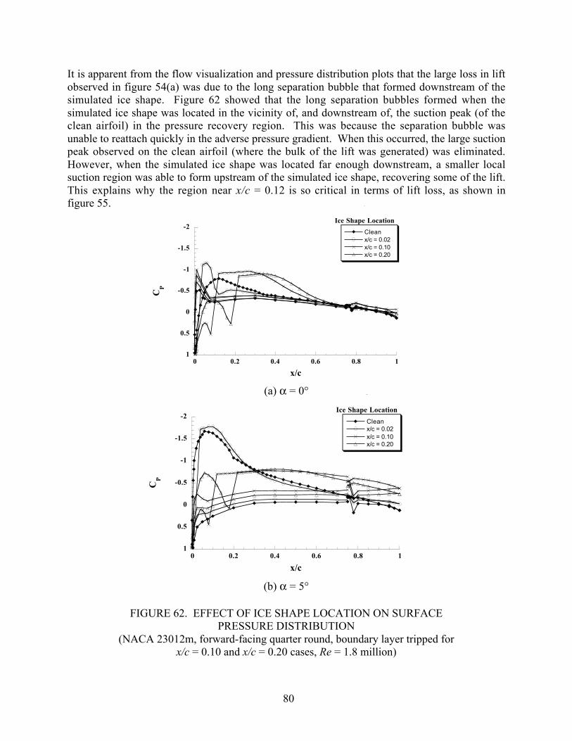
80

It is apparent from the flow visualization and pressure distribution plots that the large loss in liftobserved in figure 54(a) was due to the long separation bubble that formed downstream of thesimulated ice shape. Figure 62 showed that the long separation bubbles formed when thesimulated ice shape was located in the vicinity of, and downstream of, the suction peak (of theclean airfoil) in the pressure recovery region. This was because the separation bubble wasunable to reattach quickly in the adverse pressure gradient. When this occurred, the large suctionpeak observed on the clean airfoil (where the bulk of the lift was generated) was eliminated.However, when the simulated ice shape was located far enough downstream, a smaller localsuction region was able to form upstream of the simulated ice shape, recovering some of the lift.This explains why the region near x/c = 0.12 is so critical in terms of lift loss, as shown infigure 55.

-2

-1.5

-1

-0.5

0

0.5

10 0.2 0.4 0.6 0.8 1

Cleanx/c = 0.02x/c = 0.10x/c = 0.20

CP

x/c

Ice Shape Location

(a) α = 0°

-2

-1.5

-1

-0.5

0

0.5

10 0.2 0.4 0.6 0.8 1

Cleanx/c = 0.02x/c = 0.10x/c = 0.20

CP

x/c

Ice Shape Location

(b) α = 5°

FIGURE 62. EFFECT OF ICE SHAPE LOCATION ON SURFACEPRESSURE DISTRIBUTION

(NACA 23012m, forward-facing quarter round, boundary layer tripped forx/c = 0.10 and x/c = 0.20 cases, Re = 1.8 million)

81

4.1.1.3 Pitching and Flap Hinge Moment Analysis.

By examining the pressure distribution, the trends seen in the integrated pitching and flap hingemoments of figure 54 can be better understood. NACA 23012 is a forward-loaded airfoil inwhich most of the lift is generated in the vicinity of the large suction peak that forms near theleading edge of the airfoil. At α = 0°, when the simulated ice shape was located at x/c = 0.10 and0.20, most of the lift was generated in the region of the long separation bubble that formeddownstream of the simulated ice shape. In fact, negative lift was generated upstream of thesimulated ice shape. Thus, it became more aft loaded than the clean airfoil. When the simulatedice shape was located at x/c = 0.02, most of the lift was also generated by the separation bubble.However, the separation bubble was very short and it was located upstream of the quarter-chordlocation, resulting in a more forward-loaded lift distribution than the clean airfoil. This can beseen in figure 54(c), which shows that at α = 0°, when the simulated ice shape was located atx/c = 0.02, Cm was more positive (or nose up) than the clean case. However, when the simulatedice shape was located at x/c = 0.10 and 0.20, the pitching moments were more negative than theclean case at this angle of attack.

Similar trends were observed at α = 5°. Figure 62(b) shows that when the simulated ice shapewas located at x/c = 0.10 and 0.20, the large suction peak near the leading edge of the airfoil wasessentially eliminated and a long separation bubble formed downstream of the simulated iceshape. Thus, the airfoil became much more aft loaded. When the simulated ice shape waslocated at x/c = 0.02, the suction peak that formed near the leading edge of the model was evenlarger than that of the clean case. Thus, the airfoil became more front loaded than the clean case.Again, the result of the large changes in the pressure distribution due to the simulated ice can beobserved in the measured pitching moments of figure 54(c).

The break in the Cm curve, as shown in figure 54(c), was due to the rapidly growing separationbubble. When the simulated ice shape was located at x/c = 0.02, the break in the Cm curveoccurred at α = 5°. This is precisely the angle of attack at which the separation bubble started togrow rapidly, as figure 61 shows. Thus, the critical angle of attack at which the pitching momentbecomes severely affected coincides with the start of the rapid bubble growth.

Figure 62(a) shows that at α = 0° the presence of the simulated ice shapes did not significantlyalter the pressure distribution over the flap. However, as shown in figure 54(d), when thesimulated ice shape was located at x/c = 0.10 and 0.20, the effect of the simulated ice shape waslarge when based on the clean value even though the changes are small in an absolute sense. Atthis angle of attack (α = 0°), the simulated ice shape “unloaded” the flap (i.e., made Ch morepositive). The relatively small absolute changes in Ch at this angle of attack may have been dueto all of the separation bubbles reattaching upstream of the flap. At α = 5°, the separation bubbledid reach the flap when the simulated ice shape was located at x/c = 0.10 and 0.20. This resultedin a much larger pressure difference between the upper and lower surface of the flap, figure62(b), when compared to the clean case. Figure 54(d) shows that at α = 5°, the Ch for x/c = 0.10and 0.20 cases were more than five times as negative as that of the clean case. When thesimulated ice shape was located at x/c = 0.02, 0.10, and 0.20, the separation bubble reached theflap at α = 6.5°, 1°, and 1°, respectively. These are approximately the angles of attack where thelarge breaks in Ch occurred. Thus from the analysis of the pressure distribution and flow

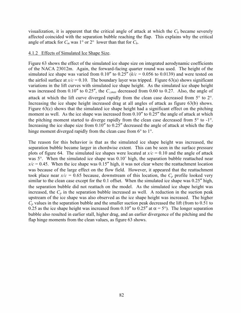
82

visualization, it is apparent that the critical angle of attack at which the Ch became severelyaffected coincided with the separation bubble reaching the flap. This explains why the criticalangle of attack for Cm was 1° or 2° lower than that for Ch.

4.1.2 Effects of Simulated Ice Shape Size.

Figure 63 shows the effect of the simulated ice shape size on integrated aerodynamic coefficientsof the NACA 23012m. Again, the forward-facing quarter round was used. The height of thesimulated ice shape was varied from 0.10″ to 0.25″ (k/c = 0.056 to 0.0139) and were tested onthe airfoil surface at x/c = 0.10. The boundary layer was tripped. Figure 63(a) shows significantvariations in the lift curves with simulated ice shape height. As the simulated ice shape heightwas increased from 0.10″ to 0.25″, the Cl,max decreased from 0.60 to 0.27. Also, the angle of

attack at which the lift curve diverged rapidly from the clean case decreased from 5° to 2°.Increasing the ice shape height increased drag at all angles of attack as figure 63(b) shows.Figure 63(c) shows that the simulated ice shape height had a significant effect on the pitchingmoment as well. As the ice shape was increased from 0.10″ to 0.25″ the angle of attack at whichthe pitching moment started to diverge rapidly from the clean case decreased from 5° to -1°.Increasing the ice shape size from 0.10″ to 0.25″ decreased the angle of attack at which the flaphinge moment diverged rapidly from the clean case from 6° to 1°.

The reason for this behavior is that as the simulated ice shape height was increased, theseparation bubble became larger in chordwise extent. This can be seen in the surface pressureplots of figure 64. The simulated ice shapes were located at x/c = 0.10 and the angle of attackwas 5°. When the simulated ice shape was 0.10˝ high, the separation bubble reattached nearx/c = 0.45. When the ice shape was 0.15″ high, it was not clear where the reattachment locationwas because of the large effect on the flow field. However, it appeared that the reattachmenttook place near x/c = 0.65 because, downstream of this location, the Cp profile looked verysimilar to the clean case except for the 0.1 offset. When the simulated ice shape was 0.25″ high,the separation bubble did not reattach on the model. As the simulated ice shape height wasincreased, the Cp in the separation bubble increased as well. A reduction in the suction peakupstream of the ice shape was also observed as the ice shape height was increased. The higherCp values in the separation bubble and the smaller suction peak decreased the lift (from to 0.51 to0.25 as the ice shape height was increased from 0.10″ to 0.25″ at α = 5°). The longer separationbubble also resulted in earlier stall, higher drag, and an earlier divergence of the pitching and theflap hinge moments from the clean values, as figure 63 shows.

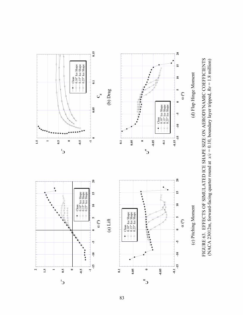
83

-1

-0.50

0.51

1.52 -1

5-1

0-5

05

1015

20

Cle

an0.

10"

Ice

Shap

e0.

15"

Ice

Shap

e0.

25"

Ice

Shap

e

Cl

α (

°)

-1

-0.50

0.51

1.5

00.

050.

10.

15

Cle

an0.

10"

Ice

Shap

e0.

15"

Ice

Shap

e0.

25"

Ice

Shap

e

Cl

Cd

(a)

Lif

t(b

) D

rag

-0.1

-0.0

50

0.050.

1

-15

-10

-50

510

1520

Cle

an0.

10"

Ice

Shap

e0.

15"

Ice

Shap

e0.

25"

Ice

Shap

e

Cm

α (

°)

-0.1

5

-0.1

-0.0

50

0.050.

1 -15

-10

-50

510

1520

Cle

an0.

10"

Ice

Shap

e0.

15"

Ice

Shap

e0.

25"

Ice

Shap

e

Ch

α (°

)

(c)

Pitc

hing

Mom

ent

(d)

Flap

Hin

ge M

omen

t

FIG

UR

E 6

3. E

FFE

CT

S O

F SI

MU

LA

TE

D I

CE

SH

APE

SIZ

E O

N A

ER

OD

YN

AM

IC C

OE

FFIC

IEN

TS

(NA

CA

230

12m

, for

war

d-fa

cing

qua

rter

rou

nd a

t x/c

= 0.

10, b

ound

ary

laye

r tr

ippe

d, Re

= 1.

8 m

illio

n)

84

-2

-1.5

-1

-0.5

0

0.5

10 0.2 0.4 0.6 0.8 1

Clean0.10" Ice Shape0.15" Ice Shape0.25" Ice Shape

CP

x/c

FIGURE 64. EFFECTS OF SIMULATED ICE SHAPE SIZE ON SURFACE PRESSURES(NACA 23012m, forward-facing quarter round at x/c = 0.10,

boundary layer tripped, α = 5° Re = 1.8 million)

Figure 65 shows the summary of the Cl,max with the three simulated ice shape sizes at various x/c

locations. Also shown in the figure is the summary of Cl,max with the 16-grit roughness (k/c =

0.0014, density = 30%) as described in section 2.1. It shows that increasing the simulated iceshape height decreased Cl,max everywhere except at the leading edge. The simulated ice shape

height did not have a large effect on Cl,max at the leading edge, with the Cl,max ranging from 0.92

to 1.01. In fact, the Cl,max for the 0.15″ simulated ice shape was higher than that of the 0.10″shape. Another interesting feature is that as the ice shape height was decreased from 0.25″ to0.10″, the location of the minimum Cl,max moved upstream from x/c = 0.12 to 0.10. This

upstream movement of the minimum Cl,max location with decreasing ice shape size is clearly

evident in the roughness data. The 16-grit roughness had an average height of 0.025″, making itapproximately 1/4 the height of the 0.10″ simulated ice shape (the smallest one that was tested).The minimum Cl,max for the roughness occurred when it was located at x/c = 0.02 and continued

the trend of the simulated ice shapes. When the roughness was placed at the leading edge, theCl,max was 0.90, which was similar to what was observed for the ice shapes. The upstream

movement of the minimum Cl,max location was probably due to the following reason. As the

simulated ice shape size was decreased, the critical location became more sensitive to thelocation of the maximum local air velocity and less on the location of the maximum adversepressure gradient. This was because as the simulated ice became smaller (with smallerseparation bubbles), the momentum removal becomes more important than the separationbubble. Since the location of the maximum local velocity is closer to the leading edge than thatof the maximum adverse pressure gradient, the ice shape location with the lowest Cl,max moved

upstream as the ice shape size was decreased.

85

0.0

0.2

0.4

0.6

0.8

1.0

1.2

1.4

1.6

0.00 0.10 0.20 0.30 0.40 0.50

Clean 0.025" Roughness0.10" Ice Shape0.15" Ice Shape0.25" Ice Shape

Cl,

max


FIGURE 65. SUMMARY OF Cl,max WITH VARIOUS SIMULATED ICE SHAPE

SIZE AND LOCATIONS(NACA 23012, forward-facing quarter round, boundary layer tripped for

case with simulated ice at x/c ≥ 0.04, Re = 1.8 million)

4.1.3 Effect of Simulated Ice Shape Geometry.

The effects of the simulated ice shape geometry on airfoil aerodynamics were also studied inorder to understand what the critical features were. Figure 66 shows the effect of variousgeometries (as shown in figure 6) on integrated aerodynamic coefficients. All of the simulationsshown in figure 66 had a height of 0.25″. Figure 66(a) shows that the forward-facing quarterround had a Cl,max of 0.27 while the backward-facing quarter round had a Cl,max of 0.34. The

backward-facing quarter round had only a slightly less severe effect on lift than the forward-facing quarter round even though the side facing the flow was much more streamlined. The halfround had a significantly higher Cl,max (0.58) than the backward-facing quarter round even

though they had an identical forward face exposed to the flow. Thus, the geometry of thedownstream side had a significant effect on lift. However, this was the case only when the faceexposed to the flow is streamlined (such as with the backward-facing quarter round and the halfround). Figure 66(a) shows that the forward-facing quarter round and the ramp shape had nearlyidentical lift curves even though they had very different downstream sides. Thus, for the twoshapes with very blunt forward faces, the shape of the backward face was not as important (forthe shapes tested).

Figure 66(b) shows the effect of the simulated ice shape geometry on drag. It shows that theforward-facing quarter round and the ramp shape had nearly identical drag polars. Of thesimulated iced cases, the half round had the least drag, followed by the backward-facing quarterround.

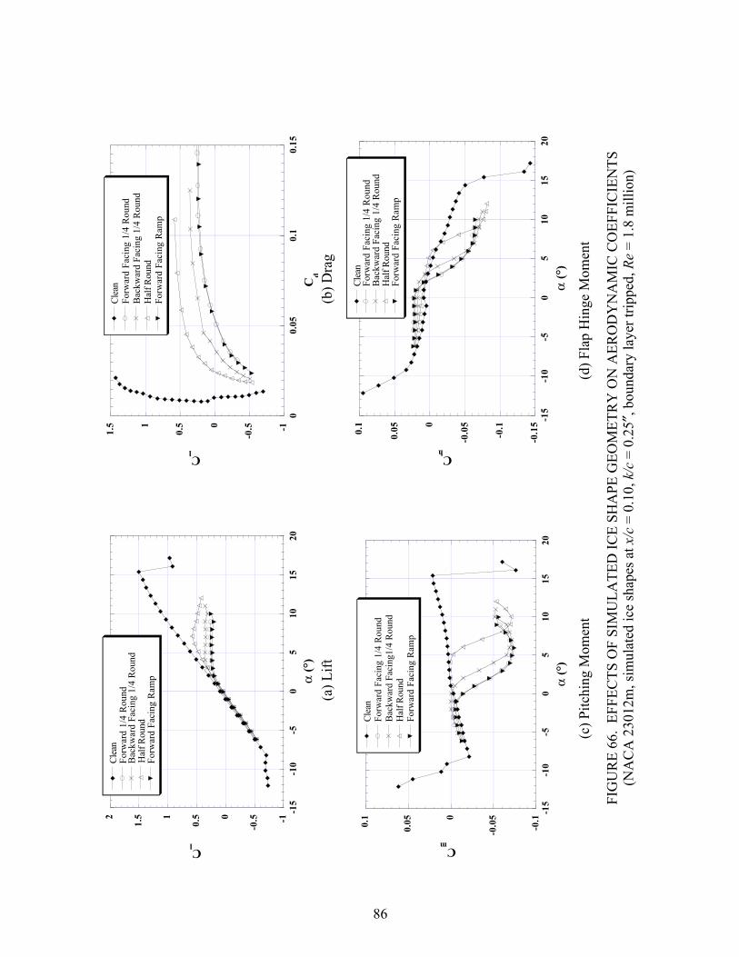
86

-1

-0.50

0.51

1.52

-15

-10

-50

510

1520

Cle

anFo

rwar

d 1/

4 R

ound

Bac

kwar

d Fa

cing

1/4

Rou

ndH

alf R

ound

Forw

ard

Faci

ng R

amp

Cl

α (

°)

-1

-0.50

0.51

1.5

00.

050.

10.

15

Cle

anFo

rwar

d Fa

cing

1/4

Rou

ndB

ackw

ard

Faci

ng 1

/4 R

ound

Hal

f Rou

ndFo

rwar

d Fa

cing

Ram

p

Cl

Cd

(a)

Lif

t(b

) D

rag

-0.1

-0.0

50

0.050.

1

-15

-10

-50

510

1520

Cle

anFo

rwar

d Fa

cing

1/4

Rou

ndB

ackw

ard

Faci

ng1/

4 R

ound

Hal

f Rou

ndFo

rwar

d Fa

cing

Ram

p

Cm

α (

°)

-0.1

5

-0.1

-0.0

50

0.050.

1 -15

-10

-50

510

1520

Cle

anFo

rwar

d Fa

cing

1/4

Rou

ndB

ackw

ard

Faci

ng 1

/4 R

ound

Hal

f Rou

ndFo

rwar

d Fa

cing

Ram

p

Ch

α (

°)

(c)

Pitc

hing

Mom

ent

(d)

Flap

Hin

ge M

omen

t

FIG

UR

E 6

6. E

FFE

CT

S O

F SI

MU

LA

TE

D I

CE

SH

APE

GE

OM

ET

RY

ON

AE

RO

DY

NA

MIC

CO

EFF

ICIE

NT

S(N

AC

A 2

3012

m, s

imul

ated

ice

shap

es a

t x/c

= 0

.10,

k/c

= 0

.25″

, bou

ndar

y la

yer

trip

ped,

Re

= 1.

8 m

illio

n)

87

Similar effects were observed for the pitching and flap hinge moments, as shown in figures 66(c)and 66(d). It shows that the backward-facing quarter round experienced Cm and Ch divergence ata higher α than the forward-facing quarter round. The half round, in turn, had the divergence ata significantly higher α than the backward-facing quarter round. Finally, the forward-facingquarter round and the ramp shape had nearly identical flap hinge curves.

4.1.4 Effects of Roughness Near Ice Shape.

SLD icing flight tests have shown the presence of roughness-type accretion upstream anddownstream of the spanwise ice shape. Thus, it was important to understand the effect of theroughness-type accretion on the iced airfoil aerodynamics. The roughness-type accretion wassimulated using 16-grit roughness tape extending upstream and downstream from the simulatedice shape (with k/c = 0.0014, density = 30%). The size and density of the roughness wasidentical to the roughness only case in figure 65. Figure 67(a) shows the result of the roughnesson lift. In all of the cases, a 0.25″ forward-facing quarter round was used at x/c = 0.10. Unlikein the other cases, the boundary layer on the upper surface was not tripped. That is the reasonwhy the no-roughness Cl,max shown in figure 67(a) was 0.37, and the Cl,max shown in figure 54(a)

was 0.27. The various extents of the roughness that were tested did produce large relativechanges in lift, but they were not large in an absolute sense since the Cl values were so low.

Figure 67(a) shows that the lowest Cl,max (0.31) resulted when the roughness extended 0.5″ in

front of the ice shape. When the chordwise roughness extent was smaller than 0.25″, most or allof the roughness was located inside the separation bubble that formed upstream of the ice shape,lessening its effect (Cl,max = 0.34). When the roughness extent was increased from 0.5″ to 2″, the

Cl,max increased from 0.31 to 0.37. This may have happened because the roughness decreased

the effective height of the ice shape by displacing the boundary layer upwards. Figure 67(a) alsoshows that when the 2″ chordwise extent roughness was placed immediately downstream of theroughness in addition to the 1″ extent upstream, the resulting Cl,max was 0.32. This was slightly

lower than the case with only the 1″ extent upstream roughness (Cl,max = 0.34). Thus, the

roughness downstream of the ice shape had a measurable effect on lift even though it wascompletely submerged within the long separation bubble that formed downstream of the iceshape.

The effect of the surface roughness on drag is shown on figure 67(b). It shows that the surfaceroughness extent did have measurable effects on drag, although they were not large. Of the casestested, the 2″ roughness extent had the least drag.

Figures 67(c) and 67(d) show the effects of surface roughness extent on the pitching and flaphinge moments. Again, they show that the surface roughness extent did not have a large effecton Cm and Ch. However, as before, the 2″ roughness extent had the least aerodynamicdegradation, as the Cm and Ch curves diverged from the clean case at a higher α than the othercases tested.

88

-0.8

-0.6

-0.4

-0.20

0.2

0.4

0.6

-10

-50

510

15

No

Rou

ghne

ss0.

25"

Ups

trea

m0.

5" U

pstr

eam

1" U

pstr

eam

2" U

pstr

eam

1" U

pstr

eam

, 2"

Dow

nstr

eam

Cl

α (

°)

Rou

ghne

ss E

xten

t

-0.8

-0.6

-0.4

-0.20

0.2

0.4

0.6

00.

050.

10.

15

No

Rou

ghne

ss0.

25"

Ups

trea

m0.

5" U

pstr

eam

1" U

pstr

eam

2" U

pstr

eam

1" U

pstr

eam

, 2"

Dow

nstr

eam

Cl

Cd

Rou

ghne

ss E

xten

t

(a)

Lif

t(b

) D

rag

-0.1

-0.0

50

0.05

-10

-50

510

15

No

Rou

ghne

ss0.

25"

Ups

trea

m0.

5" U

pstr

eam

1" U

pstr

eam

2" U

pstr

eam

1" U

pstr

eam

, 2"

Dow

nstr

eam

Cm

α (

°)

Rou

ghne

ss E

xten

t

-0.1

-0.0

50

0.05

-10

-50

510

15

No

Rou

ghne

ss0.

25"

Ups

trea

m0.

5" U

pstr

eam

1" U

pstr

eam

2" U

pstr

eam

1" U

pstr

eam

,2"

Dow

nstr

eam

Ch

α (

°)

Rou

ghne

ss E

xten

t

(c)

Pitc

hing

Mom

ent

(d)

Flap

Hin

ge M

omen

t

FIG

UR

E 6

7. E

FFE

CT

S O

F SU

RFA

CE

RO

UG

HN

ESS

IN

AD

DIT

ION

TO

SIM

UL

AT

ED

IC

E S

HA

PE O

NA

ER

OD

YN

AM

IC C

OE

FFIC

IEN

TS

(NA

CA

230

12m

, 0.2

5″ f

orw

ard-

faci

ng q

uart

er r

ound

at x/c

= 0

.10,

Re

= 1.

8 m

illio

n)

89

4.1.5 Effects of Spanwise Gaps.

In SLD aircraft icing tests [71], the spanwise ice accretion was observed to partially shed,leaving spanwise gaps. This causes the ice accretion and the associated flow field to be stronglythree-dimensional. Because of this, cases were run in order to simulate the ice accretion afterpartial shedding. The baseline 0.25″ forward-facing quarter round was tested with nominalspanwise gaps of 2.5″ and 5″. The simulated ice accretion span was kept at 6″. The schematicsof the spanwise gaps are shown in figure 15. The model on the left has 2.5″ spanwise gaps andthe model on the right has 5″ spanwise gaps. The direction of the flow is from the left to theright. This particular arrangement was chosen in order to keep one of the simulated ice shapespans over the model’s surface taps.

FIGURE 68. SPANWISE GAP GEOMETRY(NACA 23012m, 0.25″ forward-facing quarter round at x/c = 0.10,

boundary layer tripped, Re = 1.8 million)

Figure 69 shows the effects of spanwise gaps on the aerodynamic coefficients. All of the datashown in this figure were derived from the force balance measurements because the pressuremeasurements cannot capture spanwise variations in highly 3-D flow. Figure 69(a) shows thatthe presence of the spanwise gaps significantly increased the lift in the nonlinear range whencompared to the full-span simulated ice case. However, the lift curves became nonlinear atnearly the same angle of attack (3°). Also, there was not a large difference in the lift curvebetween the 2.5″ and 5″ gap cases (the 5″ gap case had slightly higher lift). Figure 69(b) showsthe effect of spanwise gaps on drag. Again, it shows that the spanwise gaps significantly reduceddrag when compared to the full-span case. The 5″ gap case had less drag than the 2.5″ casebecause it had less flow blockage.

Figures 69(c) and 69(d) show the effect of the spanwise gaps on pitching and flap hingemoments. The gaps significantly delayed the onset of the divergence of Cm and Ch from theclean model values. The divergence in Cm (for both 2.5″ and 5″ gap cases) occurred at α = 4°,instead of α = 0° for the full-span case. The divergence in Ch occurred at α = 4°, instead ofα = 1°.

90

-1

-0.50

0.51

1.5

-15

-10

-50

510

1520

Cle

anN

o G

ap2.

5" G

ap5"

Gap

Cl

α (°

)

-1

-0.50

0.51

1.5

00.

050.

10.

15

Cle

anN

o G

ap2.

5" G

ap5"

Gap

Cl

Cd

(a)

Lif

t(b

) D

rag

-0.1

-0.0

50

0.050.

1

-15

-10

-50

510

1520

Cle

anN

o G

ap2.

5" G

ap5"

Gap

Cm

α (

°)

-0.1

5

-0.1

-0.0

50

0.050.1

-15

-10

-50

510

1520

Cle

anN

o G

ap2.

5" G

ap5"

Gap

Ch

α (

°)

(c)

Pitc

hing

Mom

ent

(d)

Flap

Hin

ge M

omen

t

FIG

UR

E 6

9. E

FFE

CT

S O

F SP

AN

WIS

E G

AP

ON

AE

RO

DY

NA

MIC

CO

EFF

ICIE

NT

S(N

AC

A 2

3012

m, 0

.25″

for

war

d-fa

cing

qua

rter

rou

nd a

t x/c

= 0

.10,

dat

a de

rive

d fr

om f

orce

bal

ance

,bo

unda

ry la

yer

trip

ped,

Re

= 1.

8 m

illio

n)

91

4.1.6 Effect of Simulated Ice Accretion on the Lower Surface.

In a typical icing encounter, ice accretes on the lower surface as well as the upper surface. Thus,the NACA 23012m was tested with the baseline 0.25″ quarter round on the upper and lowersurface. Figure 70 shows the aerodynamic coefficients with the simulated ice shape placed atx/c = 0.10 on the upper and lower surfaces. The boundary layer was tripped on both upper andlower surfaces. The lift and pitching moment data shown were derived from the force-balancemeasurements. This was because when the simulated ice shape was located at x/c = 0.10 on thelower surface, there were not enough pressure taps left available on the lower surface toaccurately generate lift and pitching moment (due to sparse pressure tap distribution on the lowersurface). The drag data, however, were still derived from the wake pressure measurements.

Figure 70(a) shows that when the simulated ice shape was located only on the lower surface, itseffect on lift much less severe than when it was located on the upper surface. The Cl,max when

the simulated ice accretion was placed only on the lower surface was 1.26. This was muchgreater than the Cl,max of 0.27 when the simulated ice shape was located on the upper surface

only. The worst lift degradation occurred when the simulated ice accretion was located on boththe upper and the lower surface, with a Cl,max of 0.21. However, the lift curve was very similar to

the case where the simulated ice accretion was located only on the upper surface. The simulatedice shape on the lower surface did not have a large effect on lift because at positive angles ofattack, the pressure gradient on the lower surface is very favorable. Thus, the separation bubbledue to the simulated ice shape was much smaller than that on the upper surface.

Figure 70(b) shows the effect of the lower surface simulated ice accretion on drag. It shows thatwhen the simulated ice accretion was located only on the upper surface, it produced largeincreases in drag only at positive lift (i.e., positive α). When the simulated ice accretion waslocated only on the lower surface, large increases in drag were observed only at negative lift.When the simulated ice shape was located at both the upper and lower surfaces, large increasesin drag were observed at both negative and positive lift (and were close to the sum of the upper-only and lower-only cases).

Figure 70(c) and 70(d) show the effect of the lower surface ice accretion on pitching and flaphinge moments. It shows that when the simulated ice accretion was located only on the lowersurface, the Cm and Ch curves were very similar to that of the clean model case. When thesimulated ice accretion was located on both the upper and lower surfaces, the Cm and Ch curveswere very similar to that of the case where the simulated ice accretion was located only on theupper surface.

92

-1

-0.50

0.51

1.5

-15

-10

-50

510

1520

Cle

anU

pper

Sur

face

Low

er S

urfa

ceU

pper

and

Low

er S

urfa

ce

Cl

α (

°)

Sim

ulat

ed I

ce S

hape

Loc

atio

n

-1

-0.50

0.51

1.5

00.

050.

10.

15

Cle

anU

pper

Sur

face

Low

er S

urfa

ceU

pper

and

Low

er S

urfa

ce

Cl

Cd

Sim

ulat

ed I

ce S

hape

Loc

atio

n

(a)

Lif

t(b

) D

rag

-0.1

-0.0

50

0.050.

1 -15

-10

-50

510

1520

Cle

anU

pper

Sur

face

Low

er S

urfa

ceU

pper

and

Low

er S

urfa

ce

Cm

α (

°)

Sim

ulat

ed I

ce S

hape

Loc

atio

n

-0.1

5

-0.1

-0.0

50

0.050.1

-15

-10

-50

510

1520

Cle

anU

pper

Sur

face

Low

er S

urfa

ceU

pper

and

Low

er S

urfa

ce

Chα

(°)

Sim

ulat

ed I

ce S

hape

Loc

atio

n

(c)

Pitc

hing

Mom

ent

(d)

Flap

Hin

ge M

omen

t

FIG

UR

E 7

0. E

FFE

CT

S O

F L

OW

ER

SU

RFA

CE

SIM

UL

AT

ED

IC

E A

CC

RE

TIO

N O

N A

ER

OD

YN

AM

IC C

OE

FFIC

IEN

TS

(NA

CA

230

12m

, 0.2

5″ f

orw

ard-

faci

ng q

uart

er r

ound

at x/c

= 0

.10.

Cl

and CM

der

ived

fro

m f

orce

bal

ance

,

boun

dary

laye

r tr

ippe

d, Re

= 1.

8 m

illio

n)

93

4.1.7 Effects of Airfoil Geometry.

The importance of airfoil geometry on iced airfoil aerodynamics was investigated by testing thesimulated ice shapes on the NLF 0414 airfoil, which has aerodynamic characteristics quitedifferent from the NACA 23012m. Studying the effect of simulated ice shapes on two verydifferent airfoils provided a clearer explanation of the aerodynamic factors that determine thecritical ice shape location.

4.1.7.1 Comparison of Clean Models.

Large differences in the iced airfoil aerodynamics between the NACA 23012m and the NLF0414 were observed. This was because these two airfoils have very different geometry andaerodynamic characteristics. Figure 71 shows the comparisons between the NACA 23012m andthe NLF 0414 geometry. The NACA 23012m was designed to provide low pitching moment bygenerating most of the lift near the leading edge. The NLF 0414, however, was designed toachieve laminar flow over the airfoil by distributing the load over a large portion of the chordand delaying the onset of pressure recovery and the accompanying large adverse pressuregradient (where transition occurs) until around 70% chord.

NACA 23012mNLF 0414

FIGURE 71. COMPARISON OF NACA 23012m AND NLF 0414 GEOMETRY

The different aerodynamic characteristics are quite apparent in the measured clean-model surfacepressure of figure 72. In this figure, the surface pressures are compared at nearly identical liftcoefficients. However, because the NLF 0414 is highly cambered, it’s α was much lower thanthat of the NACA 23012m. On the NACA 23012m, there is a strong suction peak centered atx/c = 0.08, followed by an adverse pressure gradient that extended to the trailing edge. On theNLF 0414, a leading-edge suction peak was not present. Instead, after the initial accelerationaround the leading edge to x/c = 0.02, the surface pressure was nearly constant (Cp ≈ -0.8) tox/c = 0.73. The pressure recovery process began at this point and the adverse pressure gradientextended from here to the trailing edge. Since the flow around the nose on the NACA 23012maccelerated to a Cp,min = -1.7 versus only -0.9 for the NLF 0414, much more pressure recoverywas required on the NACA 23012m airfoil.

94

-2

-1.5

-1

-0.5

0

0.5

10 0.2 0.4 0.6 0.8 1

NACA 23012mNLF 0414

CP

x/c

FIGURE 72. COMPARISON OF NACA 23012m AND NLF 0414 CLEAN MODELPRESSURE DISTRIBUTION

4.1.7.2 Effect of Ice shape Locations.

All of the results in this section were with the 0.25″ forward-facing quarter-round ice shapesimulation. The boundary layer was tripped at x/c = 0.02 on the upper surface and x/c = 0.05 onthe lower surface. The boundary layer was not tripped for the clean model or when the ice shapewas located at x/c = 0.02. The Reynolds number was 1.8 million.

The differences in the airfoil geometry (and the resulting clean airfoil aerodynamiccharacteristics) between the NACA 23012m and NLF 0414 led to large differences in behaviorwith simulated ice shapes. Figure 73 shows the effect of simulated ice shape on the lift of thetwo airfoils. Varying the ice shape location from x/c = 0.02 to 0.20 had large effects on the liftof the NACA 23012m (figure 73(a)). The loss in lift was most severe when the ice shape waslocated at x/c = 0.10 (with Cl,max = 0.27). When the ice shape was located at x/c = 0.02, Cl,max

was approximately doubled.

Figure 73(b) shows the effect of simulated ice on the lift of the NLF 0414. When the simulatedice shape location was varied from x/c = 0.02 to 0.20, the lift curves did not vary significantly,with only slight changes in the Cl,max and αstall. The maximum lift was also much higher than on

the NACA 23012m, with a typical value of 0.70. When the ice shape was located at x/c = 0.40,the lift curve was significantly different as it did not have a clearly defined Cl,max. Instead, there

was an inflection in the lift curve at α = 0° due to the separation of the flow downstream of thesimulated ice shape.

95

-1

-0.5

0

0.5

1

1.5

2

-15 -10 -5 0 5 10 15 20

Cleanx/c = 0.02x/c = 0.10x/c = 0.20

Cl

α (°)

(a) NACA 23012m

-1

-0.5

0

0.5

1

1.5

2

-15 -10 -5 0 5 10 15 20

Cleanx/c = 0.02x/c = 0.10x/c = 0.20x/c = 0.40

Cl

α (°)

(b) NLF 0414

FIGURE 73. EFFECT OF SIMULATED ICE SHAPE LOCATION ON LIFT(0.25″ forward-facing quarter round, Re = 1.8 × 106, boundary layer tripped)

The large differences between the NACA 23012m and NLF 0414 airfoils can also be seen infigure 74, a summary of Cl,max as a function of ice shape location. The lowest Cl,max for the

NACA 23012m was 0.25 (an 83% reduction from the clean value) when the simulated ice shapewas located at x/c = 0.12. Thus, this was the critical ice shape location on the NACA 23012m asthe maximum lift increased rapidly as the simulated ice was moved upstream and downstream ofthis location. Figure 74 shows that on the NLF 0414, the variations in the ice shape location didnot have a large effect on Cl,max between x/c = 0.02 and x/c = 0.20. The Cl,max varied only

between 0.68 and 0.79 when the ice shape was located in this region. These values were muchhigher than those observed for the NACA 23012m. When the simulated ice shape was located atx/c = 0.30, the Cl,max dropped to 0.58 and then to 0.21 at x/c = 0.50. However, the lift curves for

these cases did not have a true Cl,max in the classical sense. Instead, only an inflection in the lift

curve was observe where the flow downstream of the simulated ice shape had failed to reattach.

96

0.0

0.2

0.4

0.6

0.8

1.0

1.2

1.4

1.6

0.00 0.05 0.10 0.15 0.20 0.25 0.30 0.35 0.40

Clean (NACA 23012m )Ice Shape (NACA 23012m)Clean (NLF 0414)Ice Shape (NLF 0414)

Cl,m

ax


FIGURE 74. SUMMARY OF Cl,max WITH 0.25″ FORWARD-FACING QUARTER ROUND

SIMULATED ICE SHAPE AT VARIOUS CHORDWISE LOCATIONS(Re = 1.8 × 106)

Figure 75 shows the drag comparisons. Both of the models showed large increases in drag withthe presence of the simulated ice shape. On the NACA 23012m, the drag increases were muchsmaller when the simulated ice shape was located at x/c = 0.02. On the NLF 0414, similar dragincreases were observed when the simulated ice shape was located at x/c = 0.02, 0.10, and 0.20.However, much large increases were observed when the simulated ice shape was located atx/c = 0.40.

-1

-0.5

0

0.5

1

1.5

0 0.05 0.1 0.15

Cleanx/c = 0.02x/c = 0.10x/c = 0.20

Cl

Cd

-1

-0.5

0

0.5

1

1.5

0 0.05 0.1 0.15

Cleanx/c = 0.02x/c = 0.10x/c = 0.20x/c = 0.40

Cl

Cd

(a) NACA 23012m (b) NLF 0414

FIGURE 75. EFFECT OF SIMULATED ICE SHAPE LOCATION ON DRAG(0.25″ forward-facing quarter round, Re = 1.8 × 106, boundary layer tripped)

The pitching moment comparisons are shown in figure 76. The simulated ice shapes causedlarge changes in the pitching moment on both airfoils. There were large breaks in the pitching

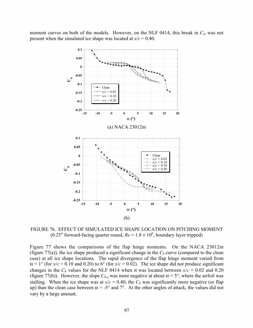
97

moment curves on both of the models. However, on the NLF 0414, this break in Cm was notpresent when the simulated ice shape was located at x/c = 0.40.

-0.25

-0.2

-0.15

-0.1

-0.05

0

0.05

0.1

-15 -10 -5 0 5 10 15 20

Cleanx/c = 0.02x/c = 0.10x/c = 0.20

Ch

α (°)

(a) NACA 23012m

-0.25

-0.2

-0.15

-0.1

-0.05

0

0.05

0.1

-15 -10 -5 0 5 10 15 20

Cleanx/c = 0.02x/c = 0.10x/c = 0.20x/c = 0.40C

h

α (°)

(b)

FIGURE 76. EFFECT OF SIMULATED ICE SHAPE LOCATION ON PITCHING MOMENT(0.25″ forward-facing quarter round, Re = 1.8 × 106, boundary layer tripped)

Figure 77 shows the comparisons of the flap hinge moments. On the NACA 23012m(figure 77(a)), the ice shape produced a significant change in the Ch curve (compared to the cleancase) at all ice shape locations. The rapid divergence of the flap hinge moment varied fromα = 1° (for x/c = 0.10 and 0.20) to 6° (for x/c = 0.02). The ice shape did not produce significantchanges in the Ch values for the NLF 0414 when it was located between x/c = 0.02 and 0.20(figure 77(b)). However, the slope Ch,α was more negative at about α = 5°, where the airfoil wasstalling. When the ice shape was at x/c = 0.40, the Ch was significantly more negative (or flapup) than the clean case between α = -5° and 7°. At the other angles of attack, the values did notvary by a large amount.

98

-0.25

-0.2

-0.15

-0.1

-0.05

0

0.05

0.1

-15 -10 -5 0 5 10 15 20

Cleanx/c = 0.02x/c = 0.10x/c = 0.20

Ch

α (°)

(a) NACA 23012m

-0.25

-0.2

-0.15

-0.1

-0.05

0

0.05

0.1

-15 -10 -5 0 5 10 15 20

Cleanx/c = 0.02x/c = 0.10x/c = 0.20x/c = 0.40C

h

α (°)

(b) NLF 0414

FIGURE 77. EFFECT OF SIMULATED ICE SHAPE LOCATION ONFLAP HINGE MOMENT

(0.25″ forward-facing quarter round, Re = 1.8 × 106, boundary layer tripped)

Figure 78 shows ∆Cd, the drag increase due to the ice shape when compared to the clean airfoil,for the 0.25″ ice shape. Figure 78(a) shows the drag increase on the NACA 23012m. It showsthat the most critical location of the simulated ice shape (in terms of ∆Cd) moved upstream withincreasing angles of attack and closely coincided with the location of the maximum local airvelocity. Figure 78(b) shows the drag increase on the NLF 0414. At angles of attack of -3° and0°, a leading-edge suction peak was not observed. Instead, the highest local air velocity occurrednear mid chord at x/c = 0.55 (for α = -3°) and 0.45 (for α = 0°). The location of maximumadverse pressure gradient was located at the trailing edge pressure recovery near x/c = 0.75.Because the simulated ice shape was not tested at x/c > 0.50, some of these points describedabove are not shown in figure 78(b). At angles of attack of 3° and 5°, a leading-edge suction

99

peak was present, with the location of the Cp,min at x/c = 0.01. The location of the maximumadverse pressure gradient was located immediately downstream of the Cp,min and not at thetrailing edge pressure recovery. At angles of attack of -3° and 0° (where there was no leading-edge suction peak on the clean model), there was a gradual increase in ∆Cd as the ice shape wasmoved downstream from the leading edge to x/c = 0.30. As the ice shape was moved furtherdownstream, ∆Cd increased at a much faster rate. At angles of attack of 3° and 5°, ∆Cd wasrelatively constant between x/c = 0.02 and x/c = 0.20, after which ∆Cd started to increase rapidly.The ∆Cd values eventually reached a maximum (at x/c = 0.4 for α = 3° and at x/c = 0.35 forα = 5°) after which they decreased. Unlike the NACA 23012m, the location of the maximumlocal air velocity was not a good indicator of the most critical simulated ice shape location.

0

0.05

0.1

0.15

0.2

0 0.05 0.1 0.15 0.2 0.25 0.3

α = 0°α = 3°α = 5°α = 8°

∆Cd (

Cd -

Cd cl

ean )




- NACA 23012m

0

0.02

0.04

0.06

0.08

0.1

0.12

0.14

0 0.1 0.2 0.3 0.4 0.5

α = -3°α = 0°α = 3°α = 5°

∆ Cd(C

d - C

d clea

n )


Maximum LocalAir Velocity onClean ModelMaximum AdversePressure Gradienton Clean Model

(b) NLF 0414

FIGURE 78. DRAG INCREASE DUE TO ICE SHAPE(0.25″ forward-facing quarter round, Re = 1.8 × 106, boundary layer tripped)

100

Figure 79 shows the lift loss ∆Cl (when compared to the clean airfoil) due to the 0.25″ ice shapesimulation. On the NACA 23012m (figure 79(a)), the most critical location of the simulatedice shape (in terms of lift loss) was between x/c = 0.10 and 0.12 and did not vary significantlywith angle of attack. This was the same location that resulted in the lowest Cl,max, as shown in

figure 74. The most critical location was situated between the locations of the maximum localair velocity and the maximum adverse pressure gradient. Thus, it did appear that the mostcritical ice shape location was related to these flow features.

0

0.1

0.2

0.3

0.4

0.5

0.6

0.7

0 0.05 0.1 0.15 0.2 0.25 0.3

α = 0°α = 3°α = 5°α = 8°



Maximum AdversePressure Gradienton Clean Model

∆ Cl(C

l clea

n - C

l )

(a) NACA 23012m

0

0.1

0.2

0.3

0.4

0.5

0.6

0 0.1 0.2 0.3 0.4 0.5

α = -3°α = 0°α = 3°α = 5°

∆ Cl(C

l clea

n - C

l )




(b) NLF 0414

FIGURE 79. LIFT LOSS DUE TO ICE SHAPE(0.25″ forward-facing quarter round, Re = 1.8 × 106, boundary layer tripped)

101

The lift loss behavior of the NLF 0414 airfoil, as shown in figure 79(b), was quite different fromthat of NACA 23012m. Figure 79(b) shows that when the ice shape was placed between theleading edge and x/c = 0.20, there was not a large variation in the lift loss. This was similar towhat was observed in the Cl,max plot of figure 74. It was only when the ice shape was located

downstream of x/c = 0.30 and closer to the adverse pressure gradient at the trailing-edge pressurerecovery that a much larger increase in the lift loss was observed. This was even the case atα = 3° and 5° where the adverse pressure gradient associated with the leading-edge suction peakwas more severe than the trailing-edge pressure recovery. Unlike the NACA 23012m, loss in liftincreased with increasing chordwise location, and the locations of maximum local air velocityand adverse pressure gradient were not proper indicators for critical locations.

4.1.7.3 Flow Field Comparisons.

The flow field of the NACA 23012m and NLF 0414 airfoils will be discussed and compared inorder to provide an explanation to the performance data of the previous section.

Figure 80(a) shows the surface pressure distribution on the NACA 23012m model with the 0.25″simulated ice shape at various chordwise locations. The angle of attack was 5°. When thesimulated ice shape was present on the airfoil, a long separation bubble usually formedimmediately downstream. Figure 80(a) shows that when the simulated ice shape was atx/c = 0.02, it was still located in a favorable pressure gradient, and the separation bubble wasrelatively short. When the simulated ice shape was located at x/c = 0.10 and 0.20, a very longseparation bubble formed downstream of the simulated ice shape. In fact, flow visualizationindicated that the bubbles did not reattach.

Figure 80(b) shows the surface pressure distribution on the NLF 0414 model with the ice shapesimulation at various chordwise locations. The angle of attack was 1°, where the clean airfoilhad a Cl similar to the NACA 23012m at α = 5°. When the ice shape was located at and

between x/c = 0.02 and 0.20, the suction region (due to separation) had similar Cp values (-1.3)and the separation length did not vary as much as it did for the NACA 23012m. The bubblelength varied from 18% chord for the x/c = 0.02 case to 28% chord for the x/c = 0.20 case. Afterthe flow had reattached, the Cp on all three cases dropped to approximately 0.50 and remainedfairly constant until the pressure recovery over the flap occurred.

When the ice shape was located at x/c = 0.40, the surface pressure distribution lookedsignificantly different than those of the other three iced cases. Also, based on the low trailing-edge pressures and flow visualization, the separation bubble was determined to not to havereattached, resulting in a separation length of 60% chord.

The reason for the similarities in the x/c = 0.02, 0.10, and 0.20 cases was that the ice shape andthe resulting separation bubble was located in a region of relatively constant pressure (on theclean model). Thus, the separation bubbles in the three cases above were all allowed to reattachin a similar pressure gradient (which happened to be nearly zero in this case). The resultingseparation bubbles all appeared similar, with relatively similar suction regions and separationlengths because the ice shape was in a similar flow field. The variation in the separation length

102

-2

-1.5

-1

-0.5

0

0.5

10 0.2 0.4 0.6 0.8 1

Cleanx/c = 0.02x/c = 0.10x/c = 0.20

CP

x/c

Ice Shape Location

(a) NACA 23012m, α = 5°

-1.5

-1

-0.5

0

0.5

10 0.2 0.4 0.6 0.8 1

Cleanx/c = 0.02x/c = 0.10x/c = 0.20x/c = 0.40

CP

x/c

Ice Shape Location

(b) NLF 0414, α = 1°

FIGURE 80. EFFECT OF SIMULATED ICE SHAPE LOCATION ON SURFACE PRESSURE

(0.25″ forward-facing quarter round, α = 1°, Re = 1.8 × 106, boundary layer tripped)

may be due to the thicker boundary layer the ice shape encountered as it was moveddownstream. The similarities ended when the ice shape was located at x/c = 0.40. Although theice shape itself was in the region of constant pressure, it was located close to the clean modelpressure recovery region (where there was a strong adverse pressure gradient). Thus, theseparation bubble was forced to reattach in an adverse pressure gradient, resulting in a trailing-edge separation.

103

The simulated ice shape affected the NACA 23012m and the NLF 0414 very differently due tothe differences in their geometries and clean airfoil aerodynamics. The NACA 23012m was amuch more forward-loaded airfoil, which resulted in a very severe adverse pressure recoverydownstream of a large, near-leading-edge suction peak. Thus, the separation bubble that formsdownstream of the simulated ice shape had to reattach in a very adverse pressure gradient. Thisresulted in very long separation bubbles with severe performance degradations. On the otherhand, the NLF 0414 had a much more evenly loaded pressure distribution. The separationbubbles that formed downstream of the simulated ice shape attached much quicker, whichresulted in much less severe performance degradation.

4.2 COMPUTATIONAL RESULTS.

4.2.1 NACA 23012m Iced Airfoil Results.

In the following, the aerodynamic influence of a forward-facing quarter-round ice shape will beconsidered. The experimental data presented in section 4.1 will be used for comparison. Thetunnel walls were modeled directly in all of these computations, so the experimental data havenot been corrected for wall interference. The data were taken for M = 0.2 and Re = 1.8 × 106

using the NACA 23012m airfoil described in section 3.1. The transition points on the uppersurface for all iced cases were chosen to be the minimum of three quantities: the ice shapelocation, the transition point predicted by XFOIL for the clean case and the trip location whichwas 2% chord for all experimental runs used for comparison in this section. On the lowersurface, again the transition point specified was the minimum of the one predicted by XFOIL forthe clean case and the trip location which was 5% for all experimental runs. As before, the codewas run for all experimental angles but only conditions which were fully converged are reportedin the figures.

Due to the presence of the ice shape and flap, a much finer grid was used for the iced-airfoilcalculations than was used in the validation calculations. Since the tunnel walls were modeled,each angle of attack required a separate grid. The initial grids contained approximately 100,000nodes and 1300 points along the airfoil surface. The grid points were clustered around the iceshape and within the separation region. The spacing of the first grid point normal to the airfoilsurface was 1 × 106 chord lengths with a 15% successive increase in grid size away from thewall. This grid was then adapted using the procedure of section 2.2.3. The final grids containedapproximately 125,000 nodes.

The computations were completed on both the Department of Aeronautical and AstronauticalEngineering (AAE) SGI workstations and the National Center for Supercomputing Applications(NCSA) SGI Power Challenge Array and Origin 2000. Iced-airfoil calculations on the SGIOrigin 2000 using 3 multigrid levels took approximately 20 seconds of CPU time per cycle. Icedcalculations required approximately 1000 cycles for convergence.

4.2.1.1 Computational Prediction Fidelity for Icing.

The ability of the current computational methodology to predict the flow field about an airfoilwith a ridge ice accretion was first tested using k/c = 0.0083 forward-facing quarter-roundprotuberance located at a chordwise location of x/c = 0.10.

104

Figures 81 through 84 plot the aerodynamic coefficients for the iced NACA 23012m. Figure 81shows the variation of lift coefficient as a function of angle of attack. At low angles of attack(α < 3°), NSU2D gave good agreement with the experimental data, although the slope wasunderpredicted by approximately 8%. Starting at 3 degrees, the computations predicted a breakin the slope and started to underpredict the experimental lift. Then as the experimental lift beganto gradually level off, the computational lift continued to increase and no noticeable maximumlift condition was seen in the NSU2D predictions. This, as is discussed later in this section, canprobably be attributed to large-scale unsteady separation bubble behavior in the measurements atfully separated angles of attack (α ≥ 3°), which the steady-state calculations cannot predict.

−20 −15 −10 −5 0 5 10 15 20

α (deg)

−1.0

−0.5

0.0

0.5

1.0

1.5

2.0

Cl

ExpNSU2D

FIGURE 81. LIFT COEFFICIENTS FOR A NACA 23012m WITH k/c = 0.0083QUARTER-ROUND ICE SHAPE LOCATED AT x/c = 0.1

Figure 82 shows the drag predictions. Despite the large amount of separation occurring on theupper surface of the airfoil, the performance of the simulations was reasonable, i.e., within10%-20% of the experimental data. The drag at the lower angles was slightly underpredicted.At the upper angles, the large increase found in the experimental drag was also seen in thecomputations, although the exact magnitude was overpredicted. This is partially attributed to thebehavior of the separation bubble predicted by the computations, which varied slightly from theactual bubble behavior expected in the experimental data.

The comparison of the predicted and experimental pitching moment is found in figure 83.Overall, NSU2D gives excellent correlation with experiment for the pitching moment. The largeincrease in negative moment caused by the growth of the separation bubble is well predictedboth qualitatively and quantitatively, although the computations predict the break at a slightlyearlier angle of attack than the experiments. The hinge moment predictions (figure 84) havesimilar agreement with the experimental data, although the earlier break is more dramatic thanfor the pitching moment.

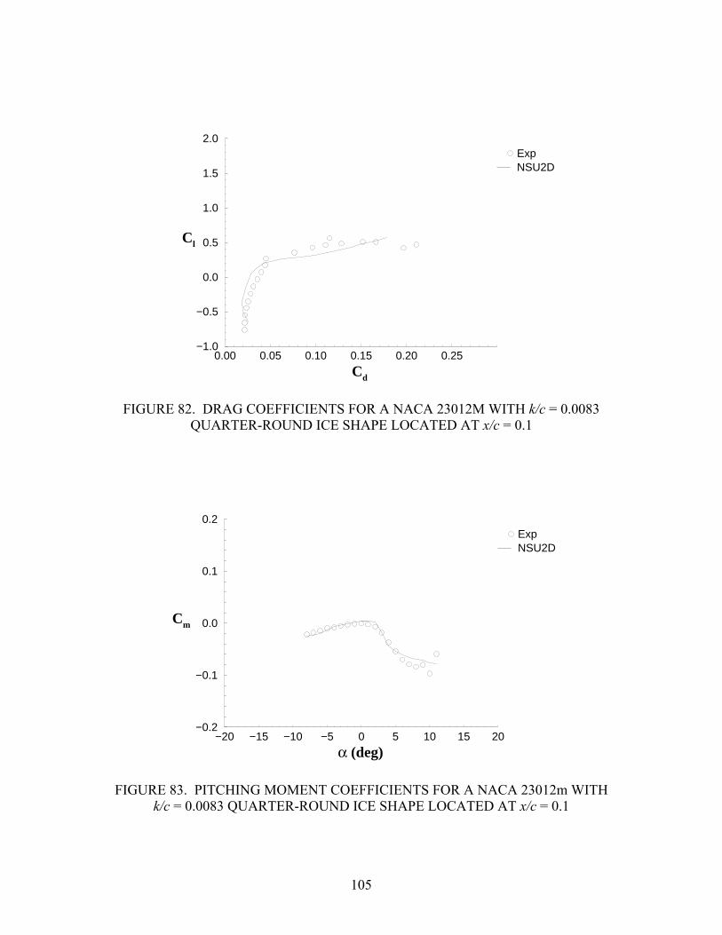
105

0.00 0.05 0.10 0.15 0.20 0.25

Cd

−1.0

−0.5

0.0

0.5

1.0

1.5

2.0

Cl

ExpNSU2D

FIGURE 82. DRAG COEFFICIENTS FOR A NACA 23012M WITH k/c = 0.0083QUARTER-ROUND ICE SHAPE LOCATED AT x/c = 0.1

−20 −15 −10 −5 0 5 10 15 20

α (deg)

−0.2

−0.1

0.0

0.1

0.2

Cm

ExpNSU2D

FIGURE 83. PITCHING MOMENT COEFFICIENTS FOR A NACA 23012m WITHk/c = 0.0083 QUARTER-ROUND ICE SHAPE LOCATED AT x/c = 0.1

106

−20 −15 −10 −5 0 5 10 15 20

α (deg)

−0.2

−0.1

0.0

0.1

0.2

Ch

ExpNSU2D

FIGURE 84. HINGE MOMENT COEFFICIENTS FOR A NACA 23012m WITH k/c = 0.0083QUARTER-ROUND ICE SHAPE LOCATED AT x/c = 0.1

Finally, we consider some of the aerodynamic characteristics responsible for the integratedquantities discussed above. Figure 85 plots selected velocity vectors within the separationbubble for α = -6°. Note that if all the velocity vectors were plotted the figure would be toodense to be clear. The velocity vectors show the large aft separation bubble extending from thetop of the ice shape with an initial expansion upwards. At this low angle of attack the separationregion was quite thin and remained fairly close to the airfoil. The small recirculation regionupstream of the ice shape showed a vertical extent which was less than the top of the ice shape, aresult which is consistent with the buff-body experiments of Winkler.

FIGURE 85. VELOCITY VECTORS AT SAMPLE LOCATIONS FOR A NACA 23012mWITH k/c = 0.0083 QUARTER-ROUND ICE SHAPE LOCATED AT x/c = 0.1 AND α = -6°

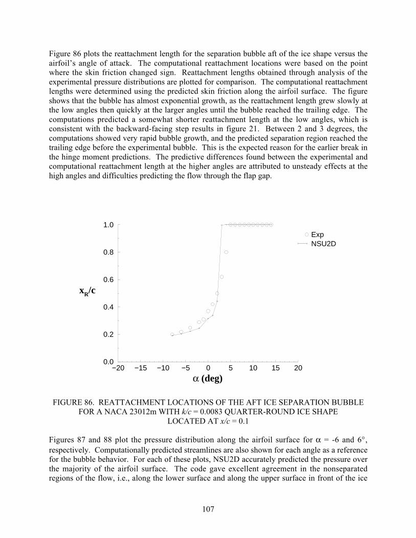
107

Figure 86 plots the reattachment length for the separation bubble aft of the ice shape versus theairfoil’s angle of attack. The computational reattachment locations were based on the pointwhere the skin friction changed sign. Reattachment lengths obtained through analysis of theexperimental pressure distributions are plotted for comparison. The computational reattachmentlengths were determined using the predicted skin friction along the airfoil surface. The figureshows that the bubble has almost exponential growth, as the reattachment length grew slowly atthe low angles then quickly at the larger angles until the bubble reached the trailing edge. Thecomputations predicted a somewhat shorter reattachment length at the low angles, which isconsistent with the backward-facing step results in figure 21. Between 2 and 3 degrees, thecomputations showed very rapid bubble growth, and the predicted separation region reached thetrailing edge before the experimental bubble. This is the expected reason for the earlier break inthe hinge moment predictions. The predictive differences found between the experimental andcomputational reattachment length at the higher angles are attributed to unsteady effects at thehigh angles and difficulties predicting the flow through the flap gap.

−20 −15 −10 −5 0 5 10 15 20

α (deg)

0.0

0.2

0.4

0.6

0.8

1.0

xR/c

ExpNSU2D

FIGURE 86. REATTACHMENT LOCATIONS OF THE AFT ICE SEPARATION BUBBLEFOR A NACA 23012m WITH k/c = 0.0083 QUARTER-ROUND ICE SHAPE

LOCATED AT x/c = 0.1

Figures 87 and 88 plot the pressure distribution along the airfoil surface for α = -6 and 6°,respectively. Computationally predicted streamlines are also shown for each angle as a referencefor the bubble behavior. For each of these plots, NSU2D accurately predicted the pressure overthe majority of the airfoil surface. The code gave excellent agreement in the nonseparatedregions of the flow, i.e., along the lower surface and along the upper surface in front of the ice

108

shape. This is especially noticeable in the α = -6° case, (figure 87) where the pressure spike atthe leading edge of the lower surface was well predicted. The code accurately predicted thepressure increase in the stagnation region ahead of the ice shape, as well as the magnitude of thesuction peak occurring downstream of the ice shape. However, similar to the results for thebackward-facing step and the glaze-iced airfoil (figure 52), NSU2D displayed a much fasterpressure recovery than the experimental data in the large separation region aft of the ice shape.This discrepancy in the separation region became more severe as the angle of attack wasincreased. This error in pressure recovery is thought to be due to the turbulence modelinadequately predicting the amount of entrainment within the shear layer. This is an area whichshould be investigated further and may require modification of the current turbulence model orfreestream turbulence values.

(a)

0.0 0.5 1.0

x/c

−4.0

−2.0

0.0

2.0

Cp

ExpNSU2D

(b)

FIGURE 87. (a) STREAMLINES AND (b) SURFACE PRESSURE DISTRIBUTIONSFOR A NACA 23012m WITH k/c = 0.0083 QUARTER-ROUND ICE SHAPE

LOCATED AT x/c = 0.1 AND α = -6

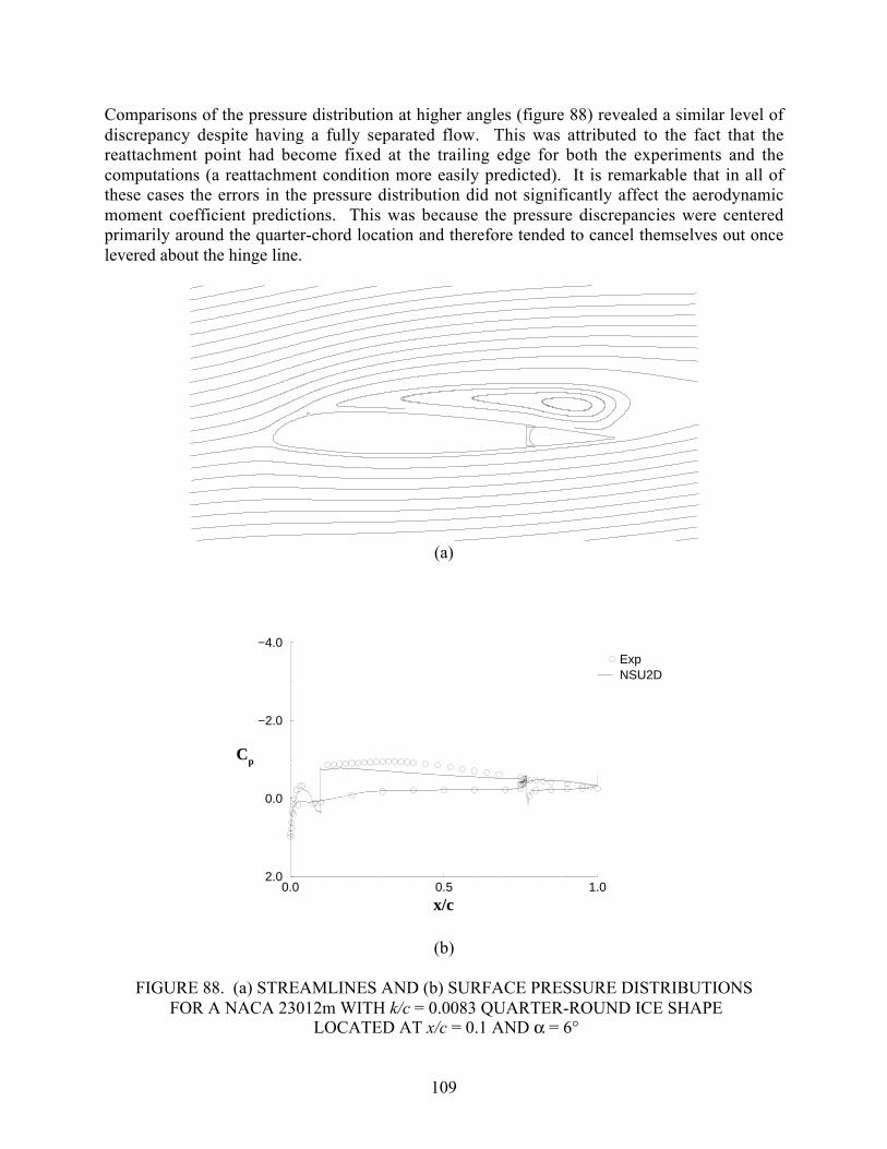
109

Comparisons of the pressure distribution at higher angles (figure 88) revealed a similar level ofdiscrepancy despite having a fully separated flow. This was attributed to the fact that thereattachment point had become fixed at the trailing edge for both the experiments and thecomputations (a reattachment condition more easily predicted). It is remarkable that in all ofthese cases the errors in the pressure distribution did not significantly affect the aerodynamicmoment coefficient predictions. This was because the pressure discrepancies were centeredprimarily around the quarter-chord location and therefore tended to cancel themselves out oncelevered about the hinge line.

(a)

0.0 0.5 1.0

x/c

−4.0

−2.0

0.0

2.0

Cp

ExpNSU2D

(b)

FIGURE 88. (a) STREAMLINES AND (b) SURFACE PRESSURE DISTRIBUTIONS FOR A NACA 23012m WITH k/c = 0.0083 QUARTER-ROUND ICE SHAPE

LOCATED AT x/c = 0.1 AND α = 6°

110

Analysis of the aerodynamic coefficients, reattachment lengths, pressure distributions, and flowfield plots indicates three general regimes of flow phenomena which can be isolated to aid infuture discussion: linear, nonlinear, and fully separated. The linear regime is associated withlow angles of attack (approximately less than 0° in this case). Here, the separation bubbleremains close to the airfoil surface and the chordwise growth of the bubble, as the angle of attackis increased, is fairly slow. At higher angles of attack (around 0-4°), the airfoil displays behaviorof the nonlinear regime, yielding a break in the aerodynamic forces and moments. Here thebubble displays rapid growth over a relatively small range of angle of attack. Unsteady flowbehavior is expected to start developing in this regime. Once the separation region reaches thetrailing edge, the airfoil is in the fully separated regime α > 4°. Here the bubble quickly beginsto extend away from the airfoil and into the outer flow field. With this type of bubble, large-scale vortex shedding is more likely to occur. This type of unsteady phenomenon can not becaptured with the current steady-state computational strategy, and therefore, the computationalresults are questionable at these angles.

The next sections will study the influence of the quarter-round simulated ice accretion by varyingits size and location. Although experimental data will also be shown, the effects predicted in thecomputations will primarily be discussed. In general, correlation between computational andexperimental data was found for each of the cases considered to be similar to that describedabove.

4.2.1.2 Effects of Variation in Size.

In the following section, the aerodynamic influence of a quarter-round ice shape is consideredcomputationally by varying its maximum height. The ice location was held constant at 10%chord and two sizes were studied: k/c = 0.0083 and k/c = 0.0139. In addition, a case with no iceshape (k/c = 0.0) which included only the boundary layer trip was used as a reference condition.The geometries of the three configurations are depicted in figure 89.

The lift curves for these configurations are shown in figure 90. The significant reduction in liftcurve slope and the dramatic reductions in maximum lift coefficient and maximum lift anglecaused by the ice shape presence were predicted reasonably well by NSU2D. However, for bothiced cases, the NSU2D predictions exhibited a weaker, although more abrupt, break in the liftcurve slope than that shown by the experiments. Although no noticeable maximum lift conditionwas seen in the NSU2D predictions, the break in the lift curve slope can be used to estimate thetrends for loss in maximum lift. Here the break does occur at an earlier angle for the larger icecase (at α = 1°) than for the smaller ice case (at α = 3°), which corresponds well with the start ofthe experimental breaks.

111

(a)

(b)

(c)

FIGURE 89. GEOMETRY OF NACA 23012m WITH AN ICE SHAPE LOCATED AT x/c = 0.1 WITH HEIGHTS (a) k/c = 0.0, (b) k/c = 0.0083, AND (c) k/c = 0.0139

112

−1.0

0.0

1.0

2.0

Cl

−20−10 0 10 20

α (deg)

k/c=0.0

ExpNSU2D

−20−10 0 10 20

α (deg)

k/c=0.0083

−20−10 0 10 20

α (deg)

k/c=0.0139

FIGURE 90. EFFECT OF SHAPE HEIGHT ON LIFT FOR ANICE SHAPE LOCATED AT x/c = 0.1

Figure 91 shows the drag predictions. The trends due to the presence and height change of theice shape were well predicted by NSU2D, considering the large amount of separation occurringfor the iced-airfoil flows. At low angles of attack, NSU2D predicted the small increase in dragas the ice size was increased, although the magnitude was slightly underpredicted. Both thecomputations and the experiments showed a significant increase in drag for the iced cases atlarge angles of attack. However, unlike the clean case, the large increases in drag for the icedcases occurred a couple of degrees before the maximum lift point.

−1.0

0.0

1.0

2.0

Cl

0.0 0.1 0.2

Cd

k/c=0.0

ExpNSU2D

0.0 0.1 0.2

Cd

k/c=0.0083

0.0 0.1 0.2

Cd

k/c=0.0139

FIGURE 91. EFFECT OF SHAPE HEIGHT ON DRAG FOR ANICE SHAPE LOCATED AT x/c = 0.1

113

Figure 92 shows the pitching moment coefficient distribution with angle of attack. The trendscaused by the presence of the ice shapes were well reproduced by NSU2D. In fact, the NSU2Dresults for the iced cases had better agreement with the experiments than the clean case (perhapsdue to the decrease in flow through the flap gap). NSU2D performed remarkably well forpredicting the strong drop-off in moment at positive angles of attack as the ice shape wasincreased in size. However, the computations did not predict the subsequent increase in momentcoefficient seen in the experimental data for angles past stall.

−0.10

−0.05

0.00

0.05

0.10

Cm

−20−10 0 10 20

α (deg)

k/c=0.0

ExpNSU2D

−20−10 0 10 20

α (deg)

k/c=0.0083

−20−10 0 10 20

α (deg)

k/c=0.0139

FIGURE 92. EFFECT OF SHAPE HEIGHT ON PITCHING MOMENT FOR AN ICE SHAPE LOCATED AT x/c = 0.1

Perhaps the most import aerodynamic coefficient with respect to aircraft control is the hingemoment. The comparison between computation and experiment of this critical parameter isshown in figure 93. Again, NSU2D successfully predicted the qualitative trends resulting fromthe presence and change in height of the ice shape. In particular, the increased drop-off in Ch athigh angles of attack was reproduced both qualitatively and quantitatively.

The pressure distribution for each of the three configurations at α = 3° is plotted in figure 94.The plots show that the presence of the ice shape caused an increase in pressure at the leadingedge, i.e., the suction peak was reduced. This created a much more rear-loaded airfoil with asubsequent change in the pitching moment and loss in lift. Also, the pressure along the lowersurface decreased as the ice shape size was increased, resulting in a further loss in lift.

114

−0.15

−0.10

−0.05

0.00

0.05

0.10

Ch

−20−10 0 10 20

α (deg)

k/c=0.0

ExpNSU2D

−20−10 0 10 20

α (deg)

k/c=0.0083

−20−10 0 10 20

α (deg)

k/c=0.0139

FIGURE 93. EFFECT OF SHAPE HEIGHT ON HINGE MOMENT FOR ANICE SHAPE LOCATED AT x/c = 0.1

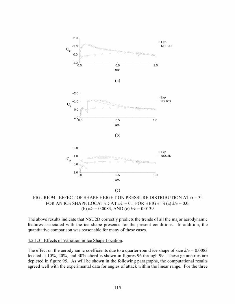
115

0.0 0.5 1.0

x/c

−2.0

−1.0

0.0

1.0

Cp

ExpNSU2D

(a)

0.0 0.5 1.0

x/c

−2.0

−1.0

0.0

1.0

Cp

ExpNSU2D

(b)

0.0 0.5 1.0

x/c

−2.0

−1.0

0.0

1.0

Cp

ExpNSU2D

(c)

FIGURE 94. EFFECT OF SHAPE HEIGHT ON PRESSURE DISTRIBUTION AT α = 3°FOR AN ICE SHAPE LOCATED AT x/c = 0.1 FOR HEIGHTS (a) k/c = 0.0,

(b) k/c = 0.0083, AND (c) k/c = 0.0139

The above results indicate that NSU2D correctly predicts the trends of all the major aerodynamicfeatures associated with the ice shape presence for the present conditions. In addition, thequantitative comparison was reasonable for many of these cases.

4.2.1.3 Effects of Variation in Ice Shape Location.

The effect on the aerodynamic coefficients due to a quarter-round ice shape of size k/c = 0.0083located at 10%, 20%, and 30% chord is shown in figures 96 through 99. These geometries aredepicted in figure 95. As will be shown in the following paragraphs, the computational resultsagreed well with the experimental data for angles of attack within the linear range. For the three

116

locations tested, the 10% chord location had the strongest influence on the aerodynamiccharacteristics of the airfoil.

(a)

(b)

(c)

FIGURE 95. GEOMETRY OF NACA 23012m WITH k/c = 0.0083 ICE SHAPE LOCATEDAT (a) x/c = 0.1, (b) x/c = 0.2, AND (c) x/c = 0.3

The effect of the protuberance at the three locations on the lift coefficient is shown in figure 96.The cases when the ice shape were located at x/c = 0.1 resulted in the largest reduction in the liftcurve slope. The 10% chord location was also the first to experience the break in the lift curve,indicating the earliest stall (although the computations did not predict the actual stall). Figure 97shows the drag predictions. Once again the 10% chord location appears to be the worst. Thiswas primarily caused by the earlier onset of stall, as there was very little difference in the drag ofthe three configurations at the lower angles of attack. The x/c = 0.1 had the most severe effect onthe pitching moment (figure 98) and hinge moment (figure 99). As the ice shape was movedrearward on the airfoil, the moment curves displayed a much more gradual break. This gradualeffect is much more desirable regarding the controllability of the aircraft.

117

−1.0

0.0

1.0

2.0

Cl

−20−10 0 10 20

α (deg)

x/c=0.1

ExpNSU2D

−20−10 0 10 20

α (deg)

x/c=0.2

−20−10 0 10 20

α (deg)

x/c=0.3

FIGURE 96. EFFECT OF SHAPE LOCATION ON LIFT FOR k/c = 0.0083 ICE SHAPE

−1.0

0.0

1.0

2.0

Cl

0.0 0.1 0.2

Cd

x/c=0.1

ExpNSU2D

0.0 0.1 0.2

Cd

x/c=0.2

0.0 0.1 0.2

Cd

x/c=0.3

FIGURE 97. EFFECT OF SHAPE LOCATION ON DRAG FOR k/c = 0.0083 ICE SHAPE

118

−0.10

−0.05

0.00

0.05

0.10

Cm

−20−10 0 10 20

α (deg)

x/c=0.1

ExpNSU2D

−20−10 0 10 20

α (deg)

x/c=0.2

−20−10 0 10 20

α (deg)

x/c=0.3

FIGURE 98. EFFECT OF SHAPE LOCATION ON PITCHING MOMENT FOR k/c = 0.0083 ICE SHAPE

−0.15

−0.10

−0.05

0.00

0.05

0.10

Ch

−20−10 0 10 20

α (deg)

x/c=0.1

ExpNSU2D

−20−10 0 10 20

α (deg)

x/c=0.2

−20−10 0 10 20

α (deg)

x/c=0.3

FIGURE 99. EFFECT OF SHAPE LOCATION ON HINGE MOMENT FORk/c = 0.0083 ICE SHAPE

119

Figure 100 displays the pressure distribution along the airfoil surface at α = 3° for the three iceshape locations. As expected, the stagnation region followed the ice shape as it was movedrearward. The airfoil with the ice shape at 10% chord did not display a suction peak at theleading edge, while the geometries with the ice shape moved farther back did possess a peak(although not as large as in the clean case seen in figure 94(a)). This appears to be the reasonwhy the 10% chord location produced the greatest decrease in lift as well as the strongestinfluence on the moment coefficients.

0.0 0.5 1.0

x/c

−2.0

−1.0

0.0

1.0

Cp

ExpNSU2D

(a)

0.0 0.5 1.0

x/c

−2.0

−1.0

0.0

1.0

Cp

ExpNSU2D

(b)

0.0 0.5 1.0

x/c

−2.0

−1.0

0.0

1.0

Cp

ExpNSU2D

(c)

FIGURE 100. EFFECT OF SHAPE LOCATION ON PRESSURE DISTRIBUTION AT α = 3°FOR k/c = 0.0083 ICE SHAPE LOCATED AT (a) x/c =0.1, (b) x/c = 0.2, AND (c) x/c = 0.3

120

Flow field analysis results are presented for the 2%, 10%, and 20% ice locations. Figures 101through 103 plot the reattchment length for the separation bubble aft of the ice shape versus theairfoil’s angle of attack. The computational reattachment lengths were determined using thepredicted skin friction along the airfoil surface. For the 2% ice location case, there is significantflow separation at the trailing edge for angle of attack as low as α = 0°. As the angle of attackincreases, the reattachment point of the bubble and the flow separation point which was initiallyat the trailing edge moves closer to each other until at about α = 7° where the two points meet.Hence, we observe a rapid break in the plot at α = 7°. Therefore, this geometry exhibits acombination of thin airfoil and trailing edge type of stall. Beyond α = 7°, the flow becameunsteady. The 10% and the 20% case exhibits a thin airfoil type of stall as seen from figures 103and 104.

Figure 104 plots the C l when the flow first becomes fully separated versus the location ofsimulated ice accretion. We see that the most detrimental effect on the lift occurs close to the10% location, as also seen from the C l - α plots. This is consistent with the experimental resultspresented in the previous section, which noted the critical location as 12% also shown in thefigure.

−20 −15 −10 −5 0 5 10 15 20

α (deg)

0.0

0.2

0.4

0.6

0.8

1.0

xR/c

NSU2D

FIGURE 101. REATTACHMENT LOCATIONS OF THE AFT ICE SEPARATIONBUBBLE FOR A NACA 23012m WITH k/c = 0.0083 QUARTER-ROUND

ICE SHAPE LOCATED AT x/c = 0.02

121

−20 −15 −10 −5 0 5 10 15 20

α (deg)

0.0

0.2

0.4

0.6

0.8

1.0

xR/c

ExpNSU2D

FIGURE 102. REATTACHMENT LOCATIONS OF THE AFT ICE SEPARATIONBUBBLE FOR A NACA 23012m WITH k/c = 0.0083 QUARTER-ROUND ICE

SHAPE LOCATED AT x/c = 0.1

−20 −15 −10 −5 0 5 10 15 20

α (deg)

0.3

0.5

0.7

0.9

xR/c

FIGURE 103. REATTACHMENT LOCATIONS OF THE AFT ICE SEPARATIONBUBBLE FOR A NACA 23012m WITH k/c = 0.0083 QUARTER-ROUND ICE


122

0.0 0.1 0.2 0.3 0.4


0.00

0.25

0.50

0.75

1.00

1.25

1.50

1.75

2.00

Cl,s

tall

Expt. Clean − Maximum Cl

NSU2D Clean − fully separated Cl

Expt. Ice Shape − Maximum Cl

NSU2D Ice Shape − fully separated Cl

FIGURE 104. LIFT COEFFICIENT FOR ANGLE OF ATTACK AT WHICH FLOW FIRST FULLY SEPARATES VS. x/c FOR A NACA 23012m AIRFOIL WITH

k/c = 0.0083 QUARTER-ROUND ICE SHAPE

4.2.1.4 Effects of Variation in Ice Shape Geometry.

Figures 105 through 108 show the effects due to variation in the shape of the ice protuberance.All of the shapes considered are located at 10% chord and have a maximum height of k/c =0.0139. Shape A is the same forward-facing quarter round discussed in section 4.2.1.1, Shape Bis a backward-facing quarter round, and Shape C is a forward-facing triangular ramp. Theshapes are presented in figure 7. The comparison with experiment for all three shapes wassimilar to that discussed previously for Shape A. As can be seen in the figures, all of the shapeshave very similar effects on the aerodynamic coefficients, but it appears that the two forward-facing shapes (A and C) have a slightly more detrimental effect on the performance than thebackward-facing quarter round (Shape B).

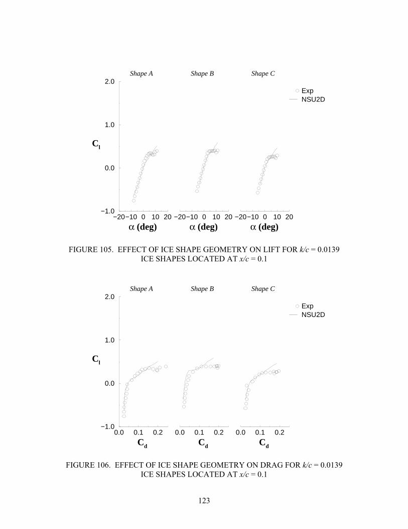
123

−1.0

0.0

1.0

2.0

Cl

−20−10 0 10 20

α (deg)

Shape A

ExpNSU2D

−20−10 0 10 20

α (deg)

Shape B

−20−10 0 10 20

α (deg)

Shape C

FIGURE 105. EFFECT OF ICE SHAPE GEOMETRY ON LIFT FOR k/c = 0.0139ICE SHAPES LOCATED AT x/c = 0.1

−1.0

0.0

1.0

2.0

Cl

0.0 0.1 0.2

Cd

Shape A

ExpNSU2D

0.0 0.1 0.2

Cd

Shape B

0.0 0.1 0.2

Cd

Shape C

FIGURE 106. EFFECT OF ICE SHAPE GEOMETRY ON DRAG FOR k/c = 0.0139ICE SHAPES LOCATED AT x/c = 0.1

124

−0.10

−0.05

0.00

0.05

0.10

Cm

−20−10 0 10 20

α (deg)

Shape A

ExpNSU2D

−20−10 0 10 20

α (deg)

Shape B

−20−10 0 10 20

α (deg)

Shape C

FIGURE 107. EFFECT OF ICE SHAPE GEOMETRY ON PITCHING MOMENT FORk/c = 0.0139 ICE SHAPES LOCATED AT x/c = 0.1

−0.15

−0.10

−0.05

0.00

0.05

0.10

Ch

−20−10 0 10 20

α (deg)

Shape A

ExpNSU2D

−20−10 0 10 20

α (deg)

Shape B

−20−10 0 10 20

α (deg)

Shape C

FIGURE 108. EFFECT OF ICE SHAPE GEOMETRY ON HINGE MOMENT FORk/c = 0.0139 ICE SHAPES LOCATED AT x/c = 0.1

125

4.2.1.5 Effects of Flap Deflection.

Calculation for the clean NACA 23012m airfoil were studied for the flap deflections of 0, 5, and10 degrees. Figures 109 through 112 show the effects due to flap deflection for the clean case.The computational predictions are compared with UIUC experimental data. We see that theNSU2D predictions for the non-iced cases exhibited good comparison with the experimentalresults, although the slope of the lift curve and maximum lift coefficient were overestimated.The code is generally able to robustly predict trends due to flap deflection on the lift curve slopeand the maximum lift for the non-iced NACA 23012m airfoil. The effect on drag, pitchingmoment, and hinge moment, due to flap deflection, show that computational predictions agreedwell with the experimental data.

The effect on the forces and moments due to variation in flap deflection is shown in figures 113through 116 for the k/c = 0.0083 iced case located at 10% chord. The computations agree wellwith the experimental data throughout the linear range. However, the prediction of lift and drag,in the nonlinear range, is only qualitatively correct.

−1.0

0.0

1.0

2.0

Cl

−20−10 0 10 20

α (deg)

δflap=0

ExpNSU2D

−20−10 0 10 20

α (deg)

δflap=5

−20−10 0 10 20

α (deg)

δflap=10

FIGURE 109. EFFECT OF FLAP DEFLECTION ON LIFT FOR k/c = 0.0

126

−1.0

0.0

1.0

2.0

Cl

0.0 0.1 0.2 0.3

Cd

δflap=0

ExpNSU2D

0.0 0.1 0.2 0.3

Cd

δflap=5

0.0 0.1 0.2 0.3

Cd

δflap=10

FIGURE 110. EFFECT OF FLAP DEFLECTION ON DRAG FOR k/c = 0.0

−0.20

−0.15

−0.10

−0.05

0.00

0.05

0.10

Cm

−20−10 0 10 20

α (deg)

δflap=0

ExpNSU2D

−20−10 0 10 20

α (deg)

δflap=5

−20−10 0 10 20

α (deg)

δflap=10

FIGURE 111. EFFECT OF FLAP DEFLECTION ON PITCHING MOMENTFOR k/c = 0.0

127

−0.25

−0.20

−0.15

−0.10

−0.05

0.00

0.05

0.10

Ch

−20−10 0 10 20

α (deg)

δflap=0

ExpNSU2D

−20−10 0 10 20

α (deg)

δflap=5

−20−10 0 10 20

α (deg)

δflap=10

FIGURE 112. EFFECT OF FLAP DEFLECTION ON HINGE MOMENT FOR k/c = 0.0

−1.0

0.0

1.0

Cl

−20−10 0 10 20

α (deg)

δflap=0

ExpNSU2D

−20−10 0 10 20

α (deg)

δflap=5

−20−10 0 10 20

α (deg)

δflap=10

FIGURE 113. EFFECT OF FLAP DEFLECTION ON LIFT FOR ICED CASE WITHk/c = 0.0083 LOCATED AT x/c = 0.1

128

−1.0

0.0

1.0

Cl

0.0 0.1 0.2

Cd

δflap=0

ExpNSU2D

0.0 0.1 0.2

Cd

δflap=5

0.0 0.1 0.2

Cd

δflap=10

FIGURE 114. EFFECT OF FLAP DEFLECTION ON DRAG FOR ICED CASE WITHk/c = 0.0083 LOCATED AT x/c = 0.1

−0.20

−0.15

−0.10

−0.05

0.00

0.05

Cm

−20−10 0 10 20

α (deg)

δflap=0

ExpNSU2D

−20−10 0 10 20

α (deg)

δflap=5

−20−10 0 10 20

α (deg)

δflap=10

FIGURE 115. EFFECT OF FLAP DEFLECTION ON PITCHING MOMENT FOR ICEDCASE WITH k/c = 0.0083 LOCATED AT x/c = 0.1

129

−0.20

−0.15

−0.10

−0.05

0.00

0.05

Ch

−20−10 0 10 20

α (deg)

δflap=0

ExpNSU2D

−20−10 0 10 20

α (deg)

δflap=5

−20−10 0 10 20

α (deg)

δflap=10

FIGURE 116. EFFECT OF FLAP DEFLECTION ON HINGE MOMENT FOR ICED CASEWITH k/c = 0.0083 LOCATED AT x/c = 0.1

4.2.1.6 Effects of Variation in Reynolds Number.

The effects on the aerodynamic performance of an iced NACA 23012m, due to variations inReynolds number, are shown in figures 117 through 120. The k/c = 0.0083 quarter-roundprotuberance located at x/c = 0.1 was chosen for this study. Since there was no experimentaldata available for the larger Reynolds numbers, only computations are presented for the higherReynolds number cases. Simulations for Reynolds numbers of 1.0, 1.8, 4, 6, and 8 million arecompared. Note, in order to save computation time, only the positive angles of attack were runfor the Re = 6 × 106 and Re = 8 × 106 and no unstructured grid adaption was used for the higherReynolds numbers. None of the aerodynamic coefficients plotted here showed a significantReynolds number influence. As such, the minor variation in the computed results for the fourReynolds numbers could be attributed to computational uncertainties in the simulations. Thelack of a Reynolds number influence is consistent with the assertion of Bragg [72] that Reynoldsnumber effects are critical for the clean case but are not discernible for the iced case. The reasonis being that the separated shear flow is insensitive to the details of the approaching boundarylayer at these conditions.

For very low angles of attack, the predictions did exhibit a slight reduction in drag at the higherReynolds number due to the decrease in skin friction (figure 118). However, the upper anglesdid not exhibit this behavior as the influence of the pressure drag began to dominate the skinfriction. Comparison of the pressure coefficient distributions for these cases (not shown) alsoreveals no significant differences caused by Reynolds number variation. It should be noted,however, that most Reynolds number effects become apparent close to stall (see section 3.3.2.1,

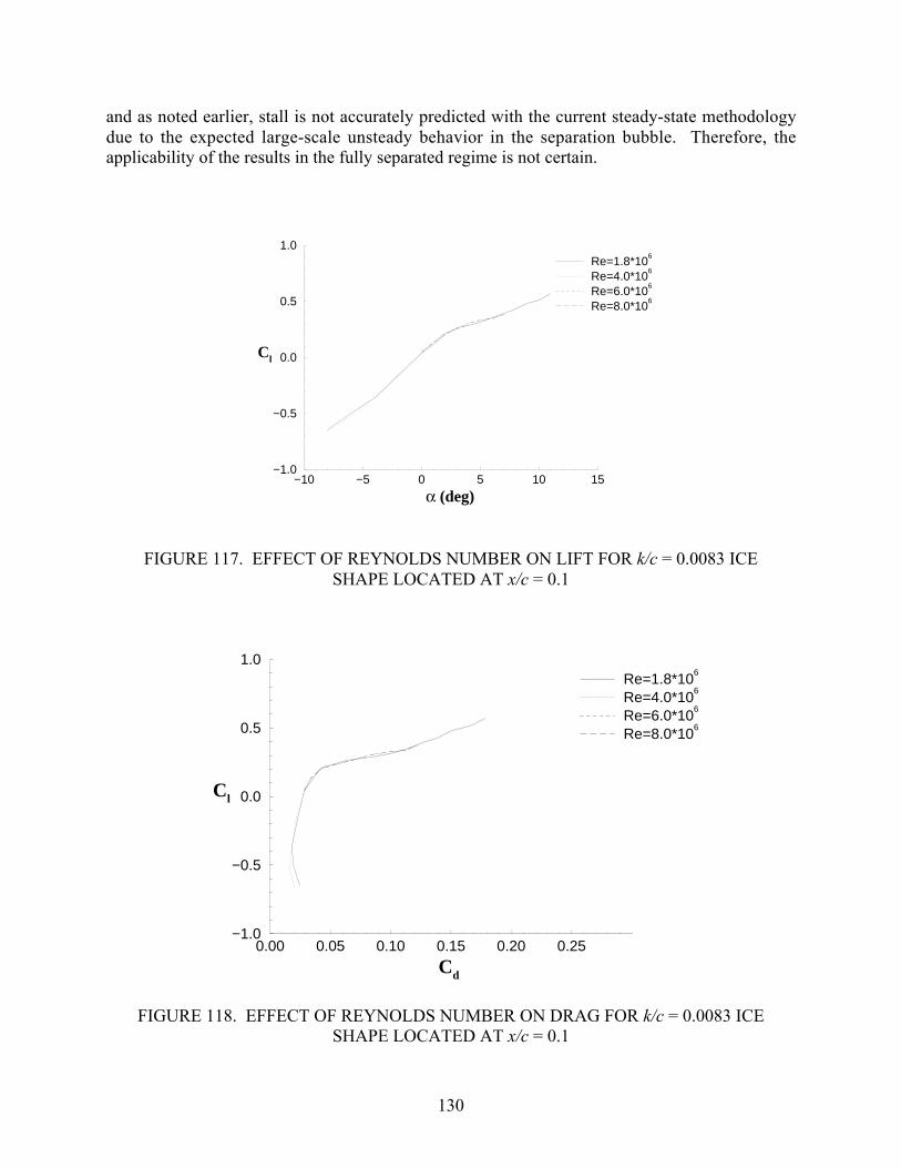
130

and as noted earlier, stall is not accurately predicted with the current steady-state methodologydue to the expected large-scale unsteady behavior in the separation bubble. Therefore, theapplicability of the results in the fully separated regime is not certain.

−10 −5 0 5 10 15

α (deg)

−1.0

−0.5

0.0

0.5

1.0

Cl

Re=1.8*106

Re=4.0*106

Re=6.0*106

Re=8.0*106

FIGURE 117. EFFECT OF REYNOLDS NUMBER ON LIFT FOR k/c = 0.0083 ICESHAPE LOCATED AT x/c = 0.1

0.00 0.05 0.10 0.15 0.20 0.25

Cd

−1.0

−0.5

0.0

0.5

1.0

Cl

Re=1.8*106

Re=4.0*106

Re=6.0*106

Re=8.0*106

FIGURE 118. EFFECT OF REYNOLDS NUMBER ON DRAG FOR k/c = 0.0083 ICESHAPE LOCATED AT x/c = 0.1

131

−10 −5 0 5 10 15

α (deg)

−0.2

−0.1

0.0

0.1

0.2

Cm

Re=1.8*106

Re=4.0*106

Re=6.0*106

Re=8.0*106

FIGURE 119. EFFECT OF REYNOLDS NUMBER ON PITCHING MOMENT FORk/c = 0.0083 ICE SHAPE LOCATED AT x/c = 0.1

−10 −5 0 5 10 15

α (deg)

−0.2

−0.1

0.0

0.1

0.2

Ch

Re=1.8*106

Re=4.0*106

Re=6.0*106

Re=8.0*106

FIGURE 120. EFFECT OF REYNOLDS NUMBER ON HINGE MOMENT FORk/c = 0.0083 ICE SHAPE LOCATED AT x/c = 0.1

132

4.2.2 Other Iced Airfoil Simulations.

The effect on the aerodynamic coefficients due to the variation in airfoil geometry was studied.Three other airfoils, in addition to the NACA 23012m, were chosen for this study. Thecoordinates for all three were provided by NASA Glenn, which has used them in other studies.The NLF 0414 was included as representative of a general aviation aircraft main wing. Abusiness jet model was included as representative of a business jet main wing. The business jetmodel is referred to as the GLC 305 in some NASA publications, although its coordinates differslightly from the GLC 305 airfoil. Finally, a large transport horizontal stabilizer (LTHS), wasincluded as representative of a commercial large transport tailplane. We wish to thank Mr. GeneAddy of NASA’s John H. Glenn Research Center at Lewis Field for providing us with the airfoilgeometries of the above airfoils. The geometries used for results in this section had a quarter-round ice shape size of k/c = 0.0083, located at 10% chord.

Figures 121 through 124 shows the surface pressure distribution for the clean case for all the fourairfoils at an equivalent C l of approximately 0.5. The business jet model and the LTHSs wererun at a Re = 8 × 106, while the data for Re = 1.8 × 106 is presented for the NACA 23012m andthe NLF 0414, since the experimental runs were conducted at this Reynolds number for theseairfoils. It can be seen from these figures that the NACA 23012m is a forward-loaded airfoilwith a light loading of the flap. The NLF 0414 has a relatively uniform chordwise loading untilthe pressure recovery near the trailing edge. Both the business jet model and the LTHSs have thesame type of loading, both are forward-loaded airfoils with a light loading of the flap in the cleancase. Both the business jet model and the LTHS airfoils have large suction peaks.

0.0 0.5 1.0

x/c

−10.0

−8.0

−6.0

−4.0

−2.0

0.0

2.0

Cp

ExpNSU2D

FIGURE 121. SURFACE PRESSURE DISTRIBUTION FOR A CLEAN NACA 23012mAIRFOIL FOR AN EQUIVALENT C l = 0.5 AT α = 4°

133

0.0 0.5 1.0

x/c

−10.0

−8.0

−6.0

−4.0

−2.0

0.0

2.0

Cp

ExpNSU2D

FIGURE 122. SURFACE PRESSURE DISTRIBUTION FOR A CLEAN NLF 0414 AIRFOILFOR AN EQUIVALENT C l = 0.5 AT α = 0°

0.0 0.5 1.0

x/c

−10.0

−8.0

−6.0

−4.0

−2.0

0.0

2.0

Cp

NSU2D

FIGURE 123. SURFACE PRESSURE DISTRIBUTION FOR A CLEAN BUSINESS JETMODEL AIRFOIL FOR AN EQUIVALENT C l = 0.5 AT α = 4°

134

0.0 0.5 1.0

x/c

−10.0

−8.0

−6.0

−4.0

−2.0

0.0

2.0

Cp

NSU2D

FIGURE 124. SURFACE PRESSURE DISTRIBUTION FOR A CLEAN LARGETRANSPORT HORIZONTAL STABILIZER AIRFOIL FOR AN EQUIVALENT

C l = 0.5 AT α = 4°

4.2.2.1 NLF Airfoil Results.

4.2.2.1.1 NLF Airfoil Results: Effect of Ice Shape Location.

Figures 125 through 128 show the effect on the aerodynamic coefficients due to variation in iceshape location for the NLF 0414 airfoil with a quarter-round ice shape size of k/c = 0.0083. Thelocations chosen for the study were x/c = 0.02, x/c = 0.1, and x/c = 0.3. The computations predicta much earlier stall and a much lower Cl. The peculiar shape of the NLF airfoil makes it a very

difficult candidate to obtain good agreement with the experimental results. The NLF 0414airfoil is highly cambered near the trailing edge, where the pressure recovery occurs. The loadis distributed over a large portion of the chord and the onset of pressure recovery and theaccompanying large adverse pressure gradient is delayed until around 70% chord. As seen fromfigure 75, NSU2D predicts a much smaller pressure spike near the leading edge in presence ofthe ice and a larger pressure recovery to occur immediately after the pressure spike compared tothe experiment. This could be a reason why there was a discrepancy in both lift and momentcoefficients, especially at higher angles of attack.

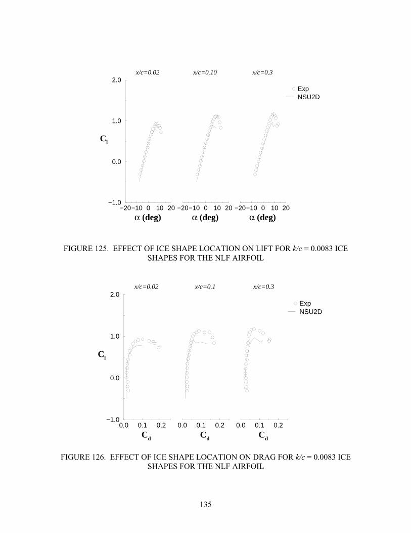
135

−1.0

0.0

1.0

2.0

Cl

−20−10 0 10 20

α (deg)

x/c=0.02

ExpNSU2D

−20−10 0 10 20

α (deg)

x/c=0.10

−20−10 0 10 20

α (deg)

x/c=0.3

FIGURE 125. EFFECT OF ICE SHAPE LOCATION ON LIFT FOR k/c = 0.0083 ICESHAPES FOR THE NLF AIRFOIL

−1.0

0.0

1.0

2.0

Cl

0.0 0.1 0.2

Cd

x/c=0.02

ExpNSU2D

0.0 0.1 0.2

Cd

x/c=0.1

0.0 0.1 0.2

Cd

x/c=0.3

FIGURE 126. EFFECT OF ICE SHAPE LOCATION ON DRAG FOR k/c = 0.0083 ICESHAPES FOR THE NLF AIRFOIL

136

−0.20

−0.15

−0.10

−0.05

0.00

Cm

−20−10 0 10 20

α (deg)

x/c=0.02

ExpNSU2D

−20−10 0 10 20

α (deg)

x/c=0.1

−20−10 0 10 20

α (deg)

x/c=0.3

FIGURE 127. EFFECT OF ICE SHAPE LOCATION ON PITCHING MOMENT FORk/c = 0.0083 ICE SHAPES FOR THE NLF AIRFOIL

−0.3

−0.2

−0.1

0.0

Ch

−10 0 10

α (deg)

x/c=0.02

ExpNSU2D

−10 0 10

α (deg)

x/c=0.1

−10 0 10

α (deg)

x/c=0.3

FIGURE 128. EFFECT OF ICE SHAPE LOCATION ON HINGE MOMENT FORk/c = 0.0083 ICE SHAPES FOR THE NLF AIRFOIL

137

The plot of predicted lift coefficients, shows that the computational predictions of the 2%,10%, and the 30% cases agreed reasonably well with the experimental results. Both thecomputations and experiments indicate large detrimental effects for all the ice shape locationstested. However, the leading-edge location appears to be the worst. The drag coefficient plot(figure 126) indicated reasonably good agreement with the experimental results at low angles ofattack. However, the angle at which the drag suddenly increases was underpredicted, especiallyfor x/c = 0.1. The break in the pitching moment curve (figure 127), occurred earlier for thecomputations. This could be because the bubble reattached earlier, compared to the experiment.The hinge moment predictions (figure 128) which is an important parameter with respect toaircraft control, agreed surprisingly well with experimental results. However, a distinctive breakwas observed in the computational predictions of the hinge moment x/c = 0.02 case, which wassubstantially delayed in the experimental results.

Figures 129 through 131 show the reattachment length for the separation bubble aft of the iceshape versus the airfoil’s angle of attack for the 2%, 10%, and 30% iced cases of the NLF 0414airfoil. The computational reattachment lengths were determined using the predicted skinfriction along the airfoil surface. The reattachment lengths grew slowly at low angles, e.g., atα < 5°, in all the three cases, then quickly grew at the larger angles until the bubble reached thetrailing edge. The plots show that the bubble almost has an exponential growth. All the caseshave a combination of a thin-airfoil type of stall and a trailing-edge type of stall. In fact, therewas trailing-edge separation even at negative angles of attack. Comparison with figure 125shows that the prediction of lift is reasonable up until full separation after which it canunderpredict the lift. This is consistent with the NACA 23012m results. From figure 132, bothcomputations and experiments indicate that for k/c = 0.0083, the near leading-edge locations,e.g., x/c = 0.02, have the most detrimental effect. However, the experimental results for k/c =0.0139 shows that the x/c = 0.3 is the most critical. As such, the simulated ice shape locationwith the largest detrimental effect is not easily determined. All the locations tested seem to havea significant detrimental effect compared to the clean case.

−20 −15 −10 −5 0 5 10 15 20

α (deg)

0.0

0.2

0.4

0.6

0.8

1.0

xR/c

NSU2D

FIGURE 129. REATTACHMENT LOCATIONS OF THE AFT ICE SEPARATIONBUBBLE FOR A NLF 0414 AIRFOIL WITH k/c = 0.0083 QUARTER-ROUND ICE


138

−20 −15 −10 −5 0 5 10 15 20

α (deg)

0.0

0.2

0.4

0.6

0.8

1.0

xR/c

NSU2D



−20 −15 −10 −5 0 5 10 15 20

α (deg)

0.0

0.2

0.4

0.6

0.8

1.0

xR/c

NSU2D



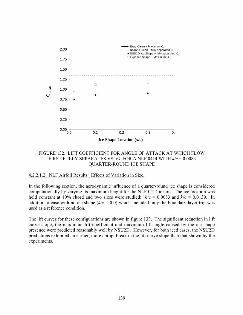
139

0.0 0.1 0.2 0.3 0.4


0.00

0.25

0.50

0.75

1.00

1.25

1.50

1.75

2.00C

l,sta

llExpt. Clean − Maximum Cl

NSU2D Clean − fully separated Cl


Expt. Ice Shape − Maximum Cl

FIGURE 132. LIFT COEFFICIENT FOR ANGLE OF ATTACK AT WHICH FLOW FIRST FULLY SEPARATES VS. x/c FOR A NLF 0414 WITH k/c = 0.0083

QUARTER-ROUND ICE SHAPE

4.2.2.1.2 NLF Airfoil Results: Effects of Variation in Size.

In the following section, the aerodynamic influence of a quarter-round ice shape is consideredcomputationally by varying its maximum height for the NLF 0414 airfoil. The ice location washeld constant at 10% chord and two sizes were studied: k/c = 0.0083 and k/c = 0.0139. Inaddition, a case with no ice shape (k/c = 0.0) which included only the boundary layer trip wasused as a reference condition.

The lift curves for these configurations are shown in figure 133. The significant reduction in liftcurve slope, the maximum lift coefficient and maximum lift angle caused by the ice shapepresence were predicted reasonably well by NSU2D. However, for both iced cases, the NSU2Dpredictions exhibited an earlier, more abrupt break in the lift curve slope than that shown by theexperiments.

140

−1.0

0.0

1.0

2.0

Cl

−20−10 0 10 20

α (deg)

k/c=0.0

ExpNSU2D

−20−10 0 10 20

α (deg)

k/c=0.0083

−20−10 0 10 20

α (deg)

k/c=0.0139

FIGURE 133. EFFECT OF ICE SHAPE ON LIFT FOR A NLF 0414 AIRFOIL WITHQUARTER-ROUND ICE SHAPE LOCATED AT x/c = 0.1

Figure 134 shows the drag predictions. The trends due to the presence and height change of theice shape were well predicted by NSU2D, considering the large amount of separation occurringfor the iced airfoil flows. At low angles of attack, NSU2D predicted the small increase in drag asthe ice size was increased, although the magnitude was slightly underpredicted. Both thecomputations and the experiments showed a significant increase in drag for the iced cases atlarge angles of attack.

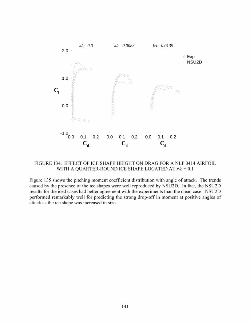
141

−1.0

0.0

1.0

2.0

Cl

0.0 0.1 0.2

Cd

k/c=0.0

ExpNSU2D

0.0 0.1 0.2

Cd

k/c=0.0083

0.0 0.1 0.2

Cd

k/c=0.0139

FIGURE 134. EFFECT OF ICE SHAPE HEIGHT ON DRAG FOR A NLF 0414 AIRFOILWITH A QUARTER-ROUND ICE SHAPE LOCATED AT x/c = 0.1

Figure 135 shows the pitching moment coefficient distribution with angle of attack. The trendscaused by the presence of the ice shapes were well reproduced by NSU2D. In fact, the NSU2Dresults for the iced cases had better agreement with the experiments than the clean case. NSU2Dperformed remarkably well for predicting the strong drop-off in moment at positive angles ofattack as the ice shape was increased in size.

142

−0.20

−0.15

−0.10

−0.05

0.00

Cm

−20−10 0 10 20

α (deg)

k/c=0.0

ExpNSU2D

−20−10 0 10 20

α (deg)

k/c=0.0083

−20−10 0 10 20

α (deg)

k/c=0.0139

FIGURE 135. EFFECT OF ICE SHAPE HEIGHT ON PITCHING MOMENT FOR A NLFAIRFOIL WITH A QUARTER-ROUND ICE SHAPE LOCATED AT x/c = 0.1

Perhaps the most important aerodynamic coefficient, with respect to aircraft control, is the hingemoment. The comparison between computation and experiment of this critical parameter isshown in figure 136. Again, NSU2D successfully predicted the qualitative trends resulting fromthe presence and change in height of the ice shape. In particular, the increased drop-off in Ch athigh angles of attack was reproduced both qualitatively and quantitatively.

In conclusion, it can be stated that the larger ice shape had a more detrimental effect (asexpected) and NSU2D predictions agree with the experimental data more closely for the icedcase of NLF 0414 than for the clean case. This is primarily due to the problem of prediction of alarge transitional flow region in the clean case. (See discussion in section 3.3.2.5.)

143

−0.3

−0.2

−0.1

0.0

Ch

−20−10 0 10 20

α (deg)

k/c=0.0

ExpNSU2D

−20−10 0 10 20

α (deg)

k/c=0.0083

−20−10 0 10 20

α (deg)

k/c=0.0139

FIGURE 136. EFFECT OF ICE SHAPE HEIGHT ON HINGE MOMENT FOR A NLF 0414AIRFOIL WITH A QUARTER-ROUND ICE SHAPE LOCATED AT x/c = 0.1

4.2.2.2 Business Jet Model Airfoil Results.

The business jet model clean airfoil is forward loaded. As observed earlier in the case of theforward-loaded NACA 23012m, a large detrimental effect of the ice shape is also expected in thecase of the business jet model.

Figures 137 through 140 show the effect of ice shape location on aerodynamic coefficients for ak/c = 0.0083 ice shape for the business jet model airfoil. The locations chosen were x/c = 0.02,x/c = 0.1, and x/c = 0.2. The clean case results are also presented for comparison. It wasobserved from the lift and drag plots that the most detrimental effect of the ice shape on lift anddrag would occur if the ice shape was placed close to x/c = 0.02. This is close to the location ofminimum pressure for the clean airfoil condition, which was further upstream compared to theNACA 23012m (see figure 121 and 123).

The pitching moment and hinge moment plots (figures 139 and 140 show that the sharpestbreaks occur for ice shape locations of x/c = 0.02 and x/c = 0.1. Consider the hinge moment plotshown in figure 140. On the clean business jet model, the flap is lightly loaded. When theseparation bubble, due to the ice shape, reaches the flap, the flap became heavily loaded andcaused a change in the hinge moment curve slope.

144

−1.5

−0.5

0.5

1.5

Cl

−10 0 10

α (deg)

Clean

NSU2D

−10 0 10

α (deg)

x/c=0.02

−10 0 10

α (deg)

x/c=0.10

−10 0 10

α (deg)

x/c=0.20

FIGURE 137. EFFECT OF ICE SHAPE LOCATION ON LIFT FOR k/c = 0.0083 ICESHAPES FOR THE BUSINESS JET MODEL AIRFOIL

−1.5

−0.5

0.5

1.5

Cl

0.0 0.1 0.2

Cd

Clean

NSU2D

0.0 0.1 0.2

Cd

x/c=0.02

0.0 0.1 0.2

Cd

x/c=0.10

0.0 0.1 0.2

Cd

x/c=0.20

FIGURE 138. EFFECT OF ICE SHAPE LOCATION ON DRAG FOR k/c = 0.0083 ICESHAPES FOR THE BUSINESS JET MODEL AIRFOIL

145

−0.15

−0.10

−0.05

0.00

Cm

−10 0 10

α (deg)

Clean

NSU2D

−10 0 10

α (deg)

x/c=0.02

−10 0 10

α (deg)

x/c=0.10

−10 0 10

α (deg)

x/c=0.20

FIGURE 139. EFFECT OF ICE SHAPE LOCATION ON PITCHING MOMENT FORk/c = 0.0083 ICE SHAPES FOR THE BUSINESS JET MODEL AIRFOIL

−0.10

−0.05

0.00

Ch

−10 0 10

α (deg)

Clean

NSU2D

−10 0 10

α (deg)

x/c=0.02

−10 0 10

α (deg)

x/c=0.10

−10 0 10

α (deg)

x/c=0.20

FIGURE 140. EFFECT OF ICE SHAPE LOCATION ON HINGE MOMENT FORk/c = 0.0083 ICE SHAPES FOR THE BUSINESS JET MODEL AIRFOIL

146

Figures 141 through 143 show the plot of the reattachment length versus the airfoil angle ofattack for the cases when the ice is located at 2%, 10%, and 20%. The 2% case has the largestdetrimental effect on C l ,max. For this location the airfoil stalls at an angle of attack of 7 degreeswhich is the lowest stall angle among all the ice shape locations on this airfoil. As with theNACA 23012m, the worst location for the lift performance is close to the peak of Cp distribution.Also, the drag increases rapidly for this C l ,max. The x/c = 0.02 iced case exhibits a combinationof a thin-airfoil type of stall and a trailing-edge type of stall; wherein, the trailing-edge separationpoint moves closer to and merges with the reattachment point of the bubble. The x/c = 0.10 icedcase also had a detrimental effect on the airfoil performance. It has a low C l when the flow firstfully separates and this occurred at an angle of attack of 8 degrees.

−20 −15 −10 −5 0 5 10 15 20

α (deg)

0.0

0.2

0.4

0.6

0.8

1.0

xR/c

NSU2D

FIGURE 141. REATTACHMENT LOCATIONS OF THE AFT ICE SEPARATIONBUBBLE FOR A BUSINESS JET MODEL AIRFOIL WITH k/c = 0.0083

QUARTER-ROUND ICE SHAPE LOCATED AT x/c = 0.02

147

−20 −15 −10 −5 0 5 10 15 20

α (deg)

0.0

0.2

0.4

0.6

0.8

1.0

xR/c

NSU2D



−20 −15 −10 −5 0 5 10 15 20

α (deg)

0.0

0.2

0.4

0.6

0.8

1.0

xR/c

NSU2D



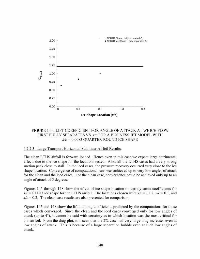
148

0.0 0.1 0.2 0.3 0.4


0.00

0.25

0.50

0.75

1.00

1.25

1.50

1.75

2.00C

l,sta

llNSU2D Clean − fully separated Cl


FIGURE 144. LIFT COEEFICIENT FOR ANGLE OF ATTACK AT WHICH FLOWFIRST FULLY SEPARATES VS. x/c FOR A BUSINESS JET MODEL WITH

k/c = 0.0083 QUARTER-ROUND ICE SHAPE

4.2.2.3 Large Transport Horizontal Stabilizer Airfoil Results.

The clean LTHS airfoil is forward loaded. Hence even in this case we expect large detrimentaleffects due to the ice shape for the locations tested. Also, all the LTHS cases had a very strongsuction peak close to stall. In the iced cases, the pressure recovery occurred very close to the iceshape location. Convergence of computational runs was achieved up to very low angles of attackfor the clean and the iced cases. For the clean case, convergence could be achieved only up to anangle of attack of 5 degrees.

Figures 145 through 148 show the effect of ice shape location on aerodynamic coefficients fork/c = 0.0083 ice shape for the LTHS airfoil. The locations chosen were x/c = 0.02, x/c = 0.1, andx/c = 0.2. The clean case results are also presented for comparison.

Figures 145 and 148 show the lift and drag coefficients predicted by the computations for thosecases which converged. Since the clean and the iced cases converged only for low angles ofattack (up to 4°), it cannot be said with certainty as to which location was the most critical forthis airfoil. From the drag plot, it is seen that the 2% case had very large drag increases even atlow angles of attack. This is because of a large separation bubble even at such low angles ofattack.

149

Figure 147 shows very sharp breaks in the pitching moment for all the iced cases. This could beattributed to the separation bubble behavior. Moreover, there was large-scale unsteadinessbeyond the angles for which the results converged. Compared to this, the hinge moment plot issmoother. This is because there is a trailing-edge separation even at low angles; hence, theseparation bubble growth and reattachment point does not affect the hinge moment curve asmuch.

−1.5

−0.5

0.5

1.5

Cl

−10 0 10

α (deg)

Clean

NSU2D

−10 0 10

α (deg)

x/c=0.02

−10 0 10

α (deg)

x/c=0.10

−10 0 10

α (deg)

x/c=0.20

FIGURE 145. EFFECT OF ICE SHAPE LOCATION ON LIFT FOR k/c = 0.0083 ICESHAPES FOR THE LARGE TRANSPORT HORIZONTAL STABILIZER

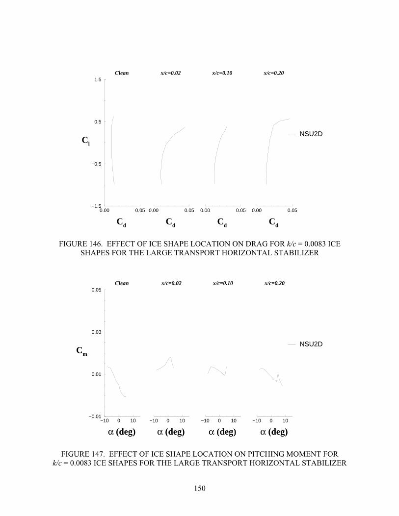
150

−1.5

−0.5

0.5

1.5

Cl

0.00 0.05

Cd

Clean

NSU2D

0.00 0.05

Cd

x/c=0.02

0.00 0.05

Cd

x/c=0.10

0.00 0.05

Cd

x/c=0.20

FIGURE 146. EFFECT OF ICE SHAPE LOCATION ON DRAG FOR k/c = 0.0083 ICESHAPES FOR THE LARGE TRANSPORT HORIZONTAL STABILIZER

−0.01

0.01

0.03

0.05

Cm

−10 0 10

α (deg)

Clean

NSU2D

−10 0 10

α (deg)

x/c=0.02

−10 0 10

α (deg)

x/c=0.10

−10 0 10

α (deg)

x/c=0.20

FIGURE 147. EFFECT OF ICE SHAPE LOCATION ON PITCHING MOMENT FORk/c = 0.0083 ICE SHAPES FOR THE LARGE TRANSPORT HORIZONTAL STABILIZER

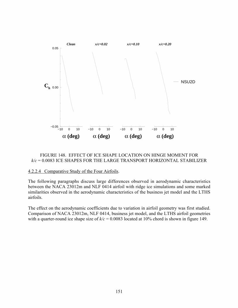
151

−0.05

0.00

0.05

Ch

−10 0 10

α (deg)

Clean

NSU2D

−10 0 10

α (deg)

x/c=0.02

−10 0 10

α (deg)

x/c=0.10

−10 0 10

α (deg)

x/c=0.20

FIGURE 148. EFFECT OF ICE SHAPE LOCATION ON HINGE MOMENT FORk/c = 0.0083 ICE SHAPES FOR THE LARGE TRANSPORT HORIZONTAL STABILIZER

4.2.2.4 Comparative Study of the Four Airfoils.

The following paragraphs discuss large differences observed in aerodynamic characteristicsbetween the NACA 23012m and NLF 0414 airfoil with ridge ice simulations and some markedsimilarities observed in the aerodynamic characteristics of the business jet model and the LTHSairfoils.

The effect on the aerodynamic coefficients due to variation in airfoil geometry was first studied.Comparison of NACA 23012m, NLF 0414, business jet model, and the LTHS airfoil geometrieswith a quarter-round ice shape size of k/c = 0.0083 located at 10% chord is shown in figure 149.

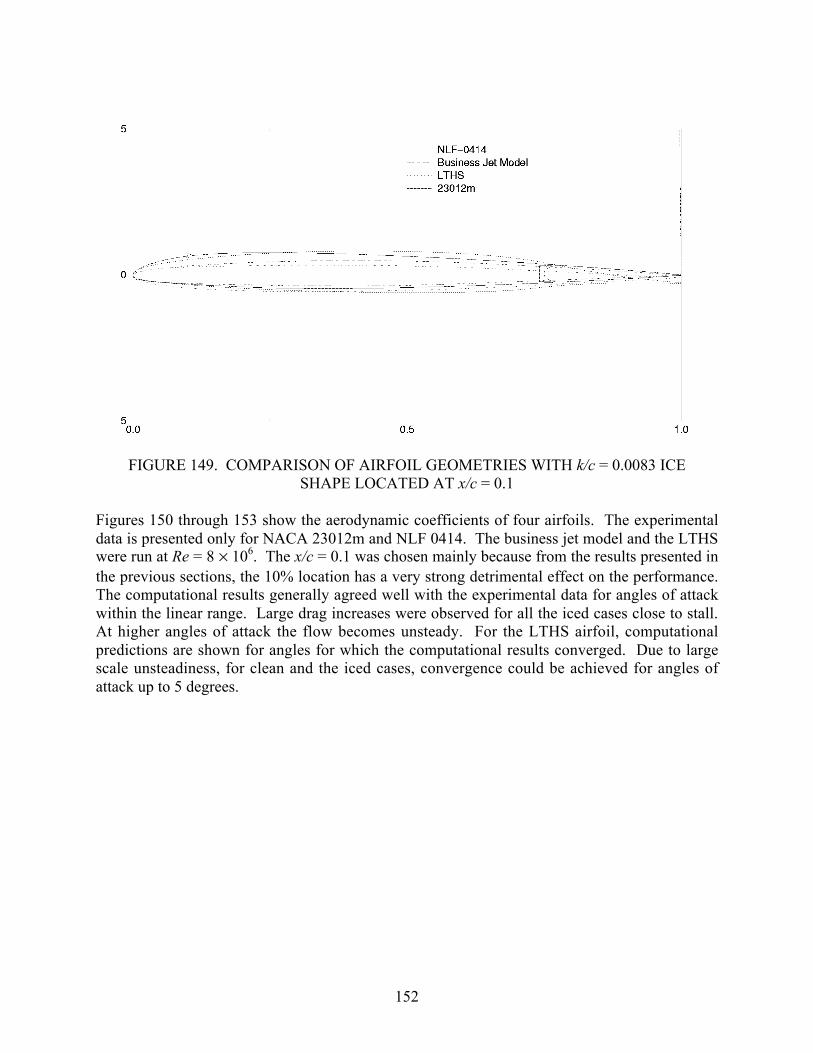
152

FIGURE 149. COMPARISON OF AIRFOIL GEOMETRIES WITH k/c = 0.0083 ICESHAPE LOCATED AT x/c = 0.1

Figures 150 through 153 show the aerodynamic coefficients of four airfoils. The experimentaldata is presented only for NACA 23012m and NLF 0414. The business jet model and the LTHSwere run at Re = 8 × 106. The x/c = 0.1 was chosen mainly because from the results presented inthe previous sections, the 10% location has a very strong detrimental effect on the performance.The computational results generally agreed well with the experimental data for angles of attackwithin the linear range. Large drag increases were observed for all the iced cases close to stall.At higher angles of attack the flow becomes unsteady. For the LTHS airfoil, computationalpredictions are shown for angles for which the computational results converged. Due to largescale unsteadiness, for clean and the iced cases, convergence could be achieved for angles ofattack up to 5 degrees.

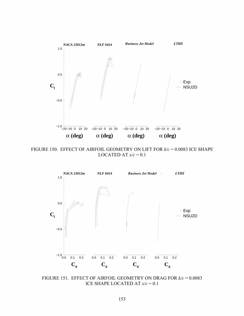
153

−1.5

−0.5

0.5

1.5

Cl

−20−10 0 10 20

α (deg)

NACA 23012m

ExpNSU2D

−20−10 0 10 20

α (deg)

NLF 0414

−20−10 0 10 20

α (deg)

GLC 305

−20−10 0 10 20

α (deg)

Boeing 757/767 HT

FIGURE 150. EFFECT OF AIRFOIL GEOMETRY ON LIFT FOR k/c = 0.0083 ICE SHAPELOCATED AT x/c = 0.1

−1.5

−0.5

0.5

1.5

Cl

0.0 0.1 0.2

Cd

NACA 23012m

ExpNSU2D

0.0 0.1 0.2

Cd

NLF 0414

0.0 0.1 0.2

Cd

GLC 305

0.0 0.1 0.2

Cd

Boeing 757/767 HT

FIGURE 151. EFFECT OF AIRFOIL GEOMETRY ON DRAG FOR k/c = 0.0083ICE SHAPE LOCATED AT x/c = 0.1

Business Jet Model LTHS


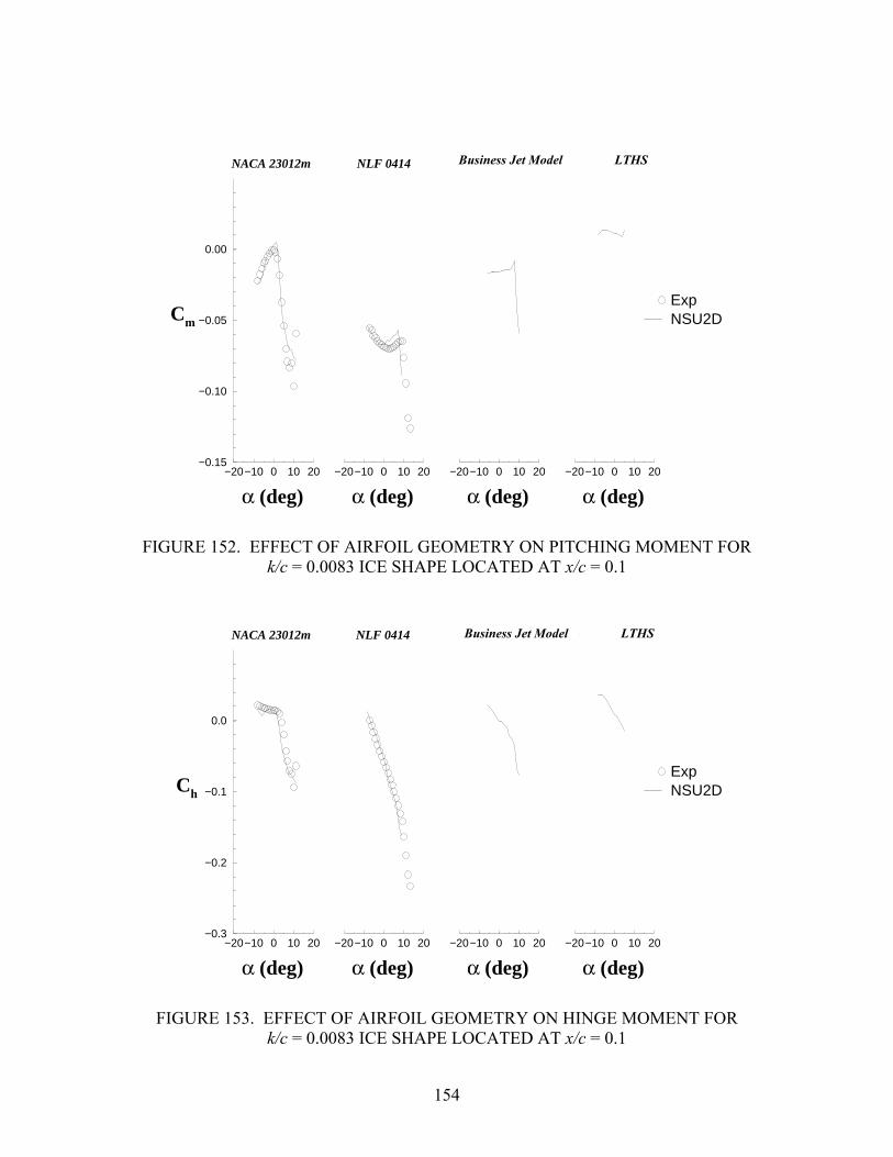
154

−0.15

−0.10

−0.05

0.00

Cm

−20−10 0 10 20

α (deg)

NACA 23012m

ExpNSU2D

−20−10 0 10 20

α (deg)

NLF 0414

−20−10 0 10 20

α (deg)

GLC 305

−20−10 0 10 20

α (deg)

Boeing 757/767 HT

FIGURE 152. EFFECT OF AIRFOIL GEOMETRY ON PITCHING MOMENT FORk/c = 0.0083 ICE SHAPE LOCATED AT x/c = 0.1

−0.3

−0.2

−0.1

0.0

Ch

−20−10 0 10 20

α (deg)

NACA 23012m

ExpNSU2D

−20−10 0 10 20

α (deg)

NLF 0414

−20−10 0 10 20

α (deg)

GLC 305

−20−10 0 10 20

α (deg)

Boeing 757/767 HT

FIGURE 153. EFFECT OF AIRFOIL GEOMETRY ON HINGE MOMENT FORk/c = 0.0083 ICE SHAPE LOCATED AT x/c = 0.1



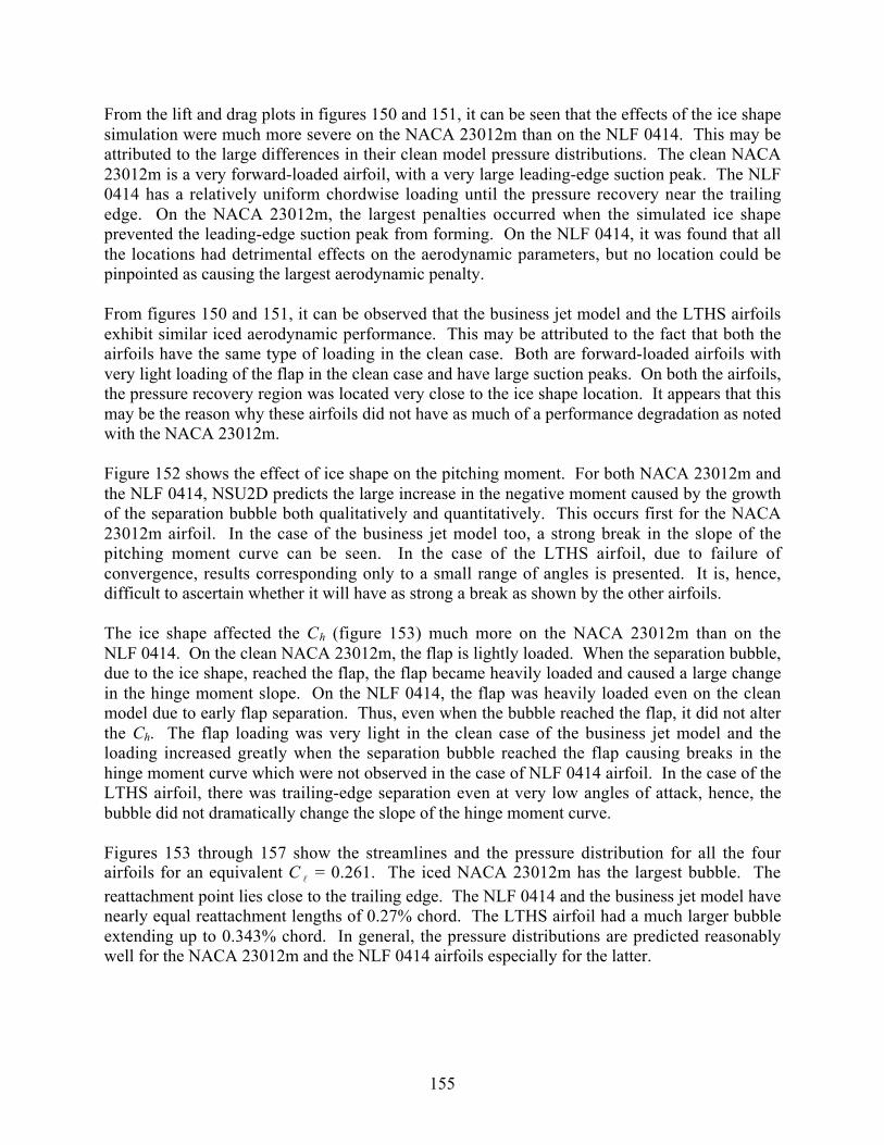
155

From the lift and drag plots in figures 150 and 151, it can be seen that the effects of the ice shapesimulation were much more severe on the NACA 23012m than on the NLF 0414. This may beattributed to the large differences in their clean model pressure distributions. The clean NACA23012m is a very forward-loaded airfoil, with a very large leading-edge suction peak. The NLF0414 has a relatively uniform chordwise loading until the pressure recovery near the trailingedge. On the NACA 23012m, the largest penalties occurred when the simulated ice shapeprevented the leading-edge suction peak from forming. On the NLF 0414, it was found that allthe locations had detrimental effects on the aerodynamic parameters, but no location could bepinpointed as causing the largest aerodynamic penalty.

From figures 150 and 151, it can be observed that the business jet model and the LTHS airfoilsexhibit similar iced aerodynamic performance. This may be attributed to the fact that both theairfoils have the same type of loading in the clean case. Both are forward-loaded airfoils withvery light loading of the flap in the clean case and have large suction peaks. On both the airfoils,the pressure recovery region was located very close to the ice shape location. It appears that thismay be the reason why these airfoils did not have as much of a performance degradation as notedwith the NACA 23012m.

Figure 152 shows the effect of ice shape on the pitching moment. For both NACA 23012m andthe NLF 0414, NSU2D predicts the large increase in the negative moment caused by the growthof the separation bubble both qualitatively and quantitatively. This occurs first for the NACA23012m airfoil. In the case of the business jet model too, a strong break in the slope of thepitching moment curve can be seen. In the case of the LTHS airfoil, due to failure ofconvergence, results corresponding only to a small range of angles is presented. It is, hence,difficult to ascertain whether it will have as strong a break as shown by the other airfoils.

The ice shape affected the Ch (figure 153) much more on the NACA 23012m than on theNLF 0414. On the clean NACA 23012m, the flap is lightly loaded. When the separation bubble,due to the ice shape, reached the flap, the flap became heavily loaded and caused a large changein the hinge moment slope. On the NLF 0414, the flap was heavily loaded even on the cleanmodel due to early flap separation. Thus, even when the bubble reached the flap, it did not alterthe Ch. The flap loading was very light in the clean case of the business jet model and theloading increased greatly when the separation bubble reached the flap causing breaks in thehinge moment curve which were not observed in the case of NLF 0414 airfoil. In the case of theLTHS airfoil, there was trailing-edge separation even at very low angles of attack, hence, thebubble did not dramatically change the slope of the hinge moment curve.

Figures 153 through 157 show the streamlines and the pressure distribution for all the fourairfoils for an equivalent C l = 0.261. The iced NACA 23012m has the largest bubble. Thereattachment point lies close to the trailing edge. The NLF 0414 and the business jet model havenearly equal reattachment lengths of 0.27% chord. The LTHS airfoil had a much larger bubbleextending up to 0.343% chord. In general, the pressure distributions are predicted reasonablywell for the NACA 23012m and the NLF 0414 airfoils especially for the latter.

156

(a)

0.0 0.5 1.0

x/c

−4.0

−2.0

0.0

2.0

Cp

ExpNSU2D

(b)

FIGURE 154. STREAMLINES AND SURFACE PRESSURE DISTRIBUTIONS FOR ANACA 23012m AIRFOIL WITH k/c = 0.0083 QUARTER-ROUND ICE SHAPE

LOCATED AT x/c = 0.1 AND α = 3°

157

x0 0.2 0.4 0.6 0.8 1

0.0 0.5 1.0

x/c

−2.0

0.0

2.0

Cp

ExpNSU2D

FIGURE 155. STREAMLINES AND SURFACE PRESSURE DISTRIBUTIONS FOR ANLF 0414 AIRFOIL WITH k/c = 0.0083 QUARTER-ROUND ICE SHAPE LOCATED

AT x/c = 0.1 AND α = -2°

158

x0 0.2 0.4 0.6 0.8 1

0.0 0.5 1.0

x/c

−4.0

−2.0

0.0

2.0

Cp

NSU2D

FIGURE 156. STREAMLINES AND SURFACE PRESSURE DISTRIBUTIONS FOR ABUSINESS JET MODEL AIRFOIL WITH k/c = 0.0083 QUARTER-ROUND

ICE SHAPE LOCATED AT x/c = 0.1 AND α = 2°

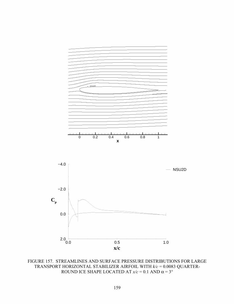
159

x0 0.2 0.4 0.6 0.8 1

0.0 0.5 1.0

x/c

−4.0

−2.0

0.0

2.0

Cp

NSU2D

FIGURE 157. STREAMLINES AND SURFACE PRESSURE DISTRIBUTIONS FOR LARGETRANSPORT HORIZONTAL STABILIZER AIRFOIL WITH k/c = 0.0083 QUARTER-

ROUND ICE SHAPE LOCATED AT x/c = 0.1 AND α = 3°

160

4.3 EXPERIMENTAL DATA CD-ROM.

All of the experimental data taken in this experiment are archived in reduced format on a CD-ROM titled UIUC/FAA SLD Experimental Data that is provided with this report. The CD-ROMis formatted for IBM-compatible computers. The data files are organized by run numbers. Eachrun number represents one angle of attack sweep (with 5 flap deflections, -10° to 10° in 5°increments) for a particular case.

There are six files associated with each run number. The first five are the separate integratedaerodynamic coefficient-reduced data files. There is a separate file for each flap deflection. Thenames of these files have the following format:

run[run number].[flap deflection]

An underscore “_” is used for negative flap angles. For example, the file for run 149 with flap =-5 would be named “run149._05”. The sixth file contains the surface pressure coefficient data.There is only one file for each run number because the Cp file contains the data for all five of theflap deflections. The names of these files have the following format:

run[run number].cp

The surface pressure file for run 149 would be named “run149.cp.”

The integrated aerodynamic coefficient data file contains both the pressure and balance data.The format for these files is shown on table 3. It is in a very simple format that does not requiremuch further explanation.

The format for the Cp data files, shown on table 4, is more complicated and requires moreexplanation. The first column is the model angle of attack and the second column is the flapangle. The first row is the x/c location of the surface pressure taps. The taps are ordered so thatit first goes from the trailing edge of the flap to the leading edge of the flap on the upper surface.Then it goes back to the trailing edge of the flap through the lower surface. It then starts at thetrailing edge of the main element and goes to the leading edge of the main element on the uppersurface. Finally, it goes to the trailing edge of the main element through the lower surface. Thesurface pressure coefficients for each angle of attack (and flap angle) are laid out as rows.

The descriptions of the run numbers are shown on tables 3 through 12. Each run contains all fiveflap deflections unless otherwise indicated.

161

TABLE 3. FORMAT OF INTEGRATED AERODYNAMIC COEFFICIENT DATA FILES

α δf Cl Pressure Cl Balance Cd Wake Cd Balance Cm Pressure Cm Balance Ch Pressure Ch Balance

-1 -5 -0.19982 -0.20051 0.01266 0.01382 0.0320174 0.029917 0.047709 0.0425-0 -5 -0.09934 -0.10109 0.01168 0.013007 0.0349076 0.031836 0.046128 0.04017

1.02 -5 -0.03239 -0.032 0.00813 0.010971 0.0434285 0.039401 0.056013 0.049012.05 -5 0.059542 0.05787 0.00792 0.010666 0.0479164 0.043759 0.059882 0.05296

… … …… …… …… …… …… …… …… ……

TABLE 4. FORMAT OF THE SURFACE PRESSURE COEFFICIENT DATA FILES

α δf 1.000 0.975 0.950 0.900 0.850 0.825 0.800

-14.14005 10 -0.391348 -0.3756646 -0.3826813 -0.4320879 -0.5211259 -0.6092398 -0.793896

-13.1566 5 -0.448579 -0.3796391 -0.3570982 -0.3573129 -0.3822463 -0.4188318 -0.4783181

-13.17717 10 -0.279054 -0.2910371 -0.3079561 -0.3683629 -0.4647658 -0.558174 -0.7547

-12.15366 0 -0.453074 -0.3471015 -0.3055085 -0.2647324 -0.2422265 -0.2366001 -0.2135846

-12.17024 5 -0.300933 -0.2794443 -0.2716719 -0.2876566 -0.3200359 -0.3620474 -0.4430255

-12.18361 10 -0.182122 -0.2173451 -0.2428358 -0.3131109 -0.4175242 -0.5141504 -0.7081167

-11.17022 -5 -0.44934 -0.3081256 -0.2457377 -0.1686718 -0.09942628 -0.06236112 0.02385377

-11.17773 0 -0.32633 -0.2634404 -0.2341093 -0.2074372 -0.1922189 -0.1912069 -0.1712768

-11.19327 5 -0.198598 -0.2035625 -0.2043917 -0.2294305 -0.2648219 -0.3181002 -0.4384505

-11.20465 10 -0.084211 -0.1393681 -0.1735512 -0.2536339 -0.3640028 -0.4626516 -0.6440821

-10.17031 -10 -0.456743 -0.2689758 -0.1864233 -0.07531165 0.03366091 0.09702635 0.2330594

-10.18207 -5 -0.346246 -0.2359919 -0.184264 -0.1196632 -0.05869595 -0.02547282 0.05577896

-10.19254 0 -0.218269 -0.184678 -0.1656577 -0.1516682 -0.1440809 -0.1465283 -0.1301576

TABLE 5. NO SIMULATED ICE AIRFOIL DATA

Airfoil Ice Shape Geometry Re (x106) Trip Run NumberNACA 23012m None 1.8 No run412NACA 23012m None 1.8 Yes run424NACA 23012m None 1.0 No run413NACA 23012m None 1.0 Yes run483NLF 0414 None 1.8 NoNLF 0414 None 1.8 Yes run301

162

TABLE 6. FORWARD-FACING QUARTER ROUND, k = 0.25″, NACA 23012m

Re (x106) Trip x/c Run Number Comments1.8 No 0 run478 flap = -10 deg only1.8 No 0 run479 flap = -5 deg only1.8 No 0 run480 flap = 0 deg only1.8 No 0 run481 flap = 5 deg only1.8 No 0 run482 flap = 10 deg only1.8 No 0.02 run4761.8 No 0.04 run5011.8 No 0.06 run5051.8 No 0.1 run5021.8 No 0.14 run5041.8 No 0.2 run5031.8 Yes 0.04 run5001.8 Yes 0.06 run4851.8 Yes 0.08 run4861.8 Yes 0.1 run4871.8 Yes 0.12 run4901.8 Yes 0.14 run4921.8 Yes 0.16 run4941.8 Yes 0.18 run4951.8 Yes 0.2 run4971.8 Yes 0.3 run4981.8 Yes 0.5 run4991 No 0 run4771 No 0.02 run4751 Yes 0.06 run4841 Yes 0.1 run4881 Yes 0.14 run4931 Yes 0.2 run496

163


Re (x106) Trip x/c Run Number Comments1.8 No 0 run4711.8 No 0.02 run4691.8 No 0.04 run4301.8 No 0.06 run4311.8 No 0.08 run4321.8 No 0.1 run4351.8 No 0.12 run4361.8 No 0.14 run4371.8 No 0.16 run4391.8 No 0.18 run4401.8 No 0.2 run4381.8 No 0.3 run4411.8 No 0.3 run442 completion of run4411.8 No 0.5 run4431.8 Yes 0.04 run4681.8 Yes 0.06 run4661.8 Yes 0.08 run4651.8 Yes 0.1 run4551.8 Yes 0.12 run4591.8 Yes 0.14 run4601.8 Yes 0.16 run4611.8 Yes 0.18 run4621.8 Yes 0.2 run4571.8 Yes 0.3 run4631.8 Yes 0.5 run4641 No 0 run472 flap = -10,-5,01 No 0 run473 flap = 5,101 No 0.02 run4701 Yes 0.06 run4671 Yes 0.1 run4561 Yes 0.12 run458

164


Re (x106) Trip x/c Run Number1.8 No 0 run5301.8 No 0.02 run5291.8 No 0.1 run5281.8 Yes 0.06 run5251.8 Yes 0.08 run5261.8 Yes 0.1 run5221.8 Yes 0.12 run5271.8 Yes 0.14 run5241.8 Yes 0.2 run523

TABLE 9. VARIOUS SIMULATED ICE SHAPE GEOMETRY, k = 0.25″,Re = 1.8 × 106, NACA 23012m

Ice Shape Geometry Trip x/c Run Number Comments

Backward-Facing 1/4 Round No 0.02 run506Backward-Facing 1/4 Round Yes 0.10 run507Backward-Facing 1/4 Round Yes 0.20 run508Forward-Facing Ramp No 0.02 run517Forward-Facing Ramp No 0.02 run518 completion of run517Forward-Facing Ramp Yes 0.10 run516Forward-Facing Ramp Yes 0.20 run515Half Round No 0.02 run519Half Round Yes 0.10 run520Half Round Yes 0.20 run521

TABLE 10. FORWARD-FACING QUARTER ROUND ON UPPER AND LOWERSURFACE OF THE MODEL AT x/c = 0.10, k = 0.25″, Re = 1.8 × 106, NACA 23012m

Upper Lower Height Re (x106) Trip x/c Run NumberNo Yes 0.25" 1.8 No 0.10 run509Yes Yes 0.25" 1.8 No 0.10 run510

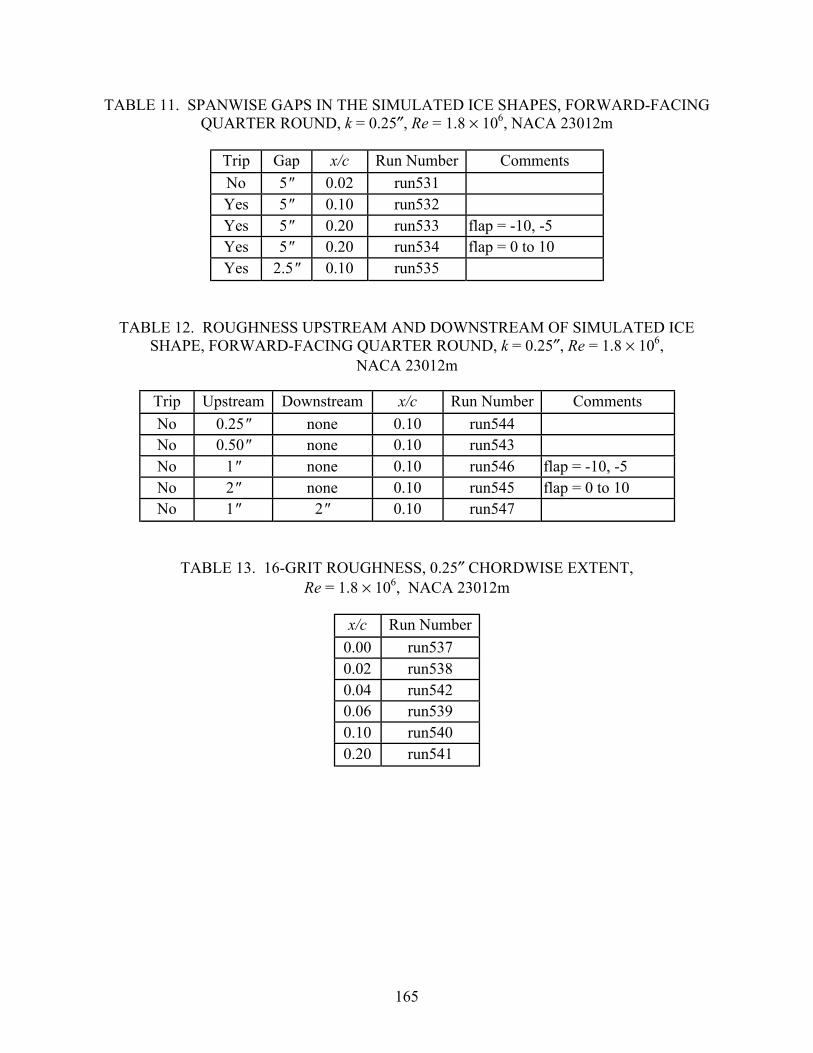
165

TABLE 11. SPANWISE GAPS IN THE SIMULATED ICE SHAPES, FORWARD-FACINGQUARTER ROUND, k = 0.25″, Re = 1.8 × 106, NACA 23012m

Trip Gap x/c Run Number CommentsNo 5" 0.02 run531Yes 5" 0.10 run532Yes 5" 0.20 run533 flap = -10, -5Yes 5" 0.20 run534 flap = 0 to 10Yes 2.5" 0.10 run535

TABLE 12. ROUGHNESS UPSTREAM AND DOWNSTREAM OF SIMULATED ICESHAPE, FORWARD-FACING QUARTER ROUND, k = 0.25″, Re = 1.8 × 106,

NACA 23012m

Trip Upstream Downstream x/c Run Number Comments

No 0.25" none 0.10 run544No 0.50" none 0.10 run543No 1" none 0.10 run546 flap = -10, -5No 2" none 0.10 run545 flap = 0 to 10No 1" 2" 0.10 run547

TABLE 13. 16-GRIT ROUGHNESS, 0.25″ CHORDWISE EXTENT,Re = 1.8 × 106, NACA 23012m

x/c Run Number

0.00 run5370.02 run5380.04 run5420.06 run5390.10 run5400.20 run541

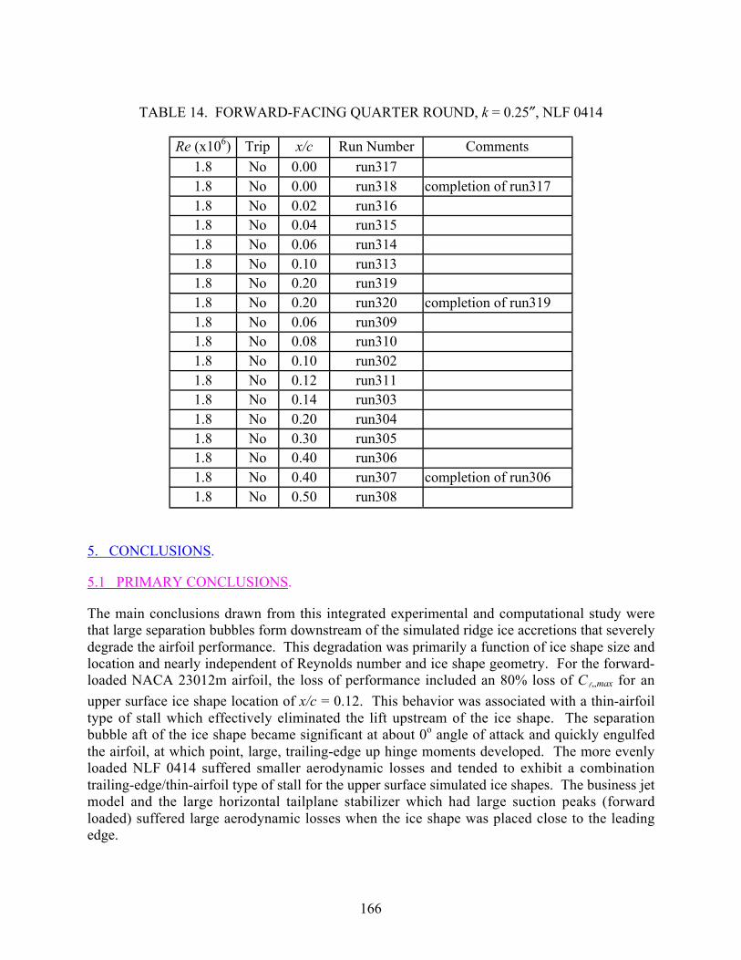
166

TABLE 14. FORWARD-FACING QUARTER ROUND, k = 0.25″, NLF 0414

Re (x106) Trip x/c Run Number Comments1.8 No 0.00 run3171.8 No 0.00 run318 completion of run3171.8 No 0.02 run3161.8 No 0.04 run3151.8 No 0.06 run3141.8 No 0.10 run3131.8 No 0.20 run3191.8 No 0.20 run320 completion of run3191.8 No 0.06 run3091.8 No 0.08 run3101.8 No 0.10 run3021.8 No 0.12 run3111.8 No 0.14 run3031.8 No 0.20 run3041.8 No 0.30 run3051.8 No 0.40 run3061.8 No 0.40 run307 completion of run3061.8 No 0.50 run308

5. CONCLUSIONS.

5.1 PRIMARY CONCLUSIONS.

The main conclusions drawn from this integrated experimental and computational study werethat large separation bubbles form downstream of the simulated ridge ice accretions that severelydegrade the airfoil performance. This degradation was primarily a function of ice shape size andlocation and nearly independent of Reynolds number and ice shape geometry. For the forward-loaded NACA 23012m airfoil, the loss of performance included an 80% loss of Cl,,max for an

upper surface ice shape location of x/c = 0.12. This behavior was associated with a thin-airfoiltype of stall which effectively eliminated the lift upstream of the ice shape. The separationbubble aft of the ice shape became significant at about 0o angle of attack and quickly engulfedthe airfoil, at which point, large, trailing-edge up hinge moments developed. The more evenlyloaded NLF 0414 suffered smaller aerodynamic losses and tended to exhibit a combinationtrailing-edge/thin-airfoil type of stall for the upper surface simulated ice shapes. The business jetmodel and the large horizontal tailplane stabilizer which had large suction peaks (forwardloaded) suffered large aerodynamic losses when the ice shape was placed close to the leadingedge.

167

In the following, additional conclusions and details are given first for the experimental study andthen for the computational study.

5.2 EXPERIMENTAL STUDY CONCLUSIONS.

An experimental study was conducted in order to understand the effects of ridge ice accretion onaircraft aerodynamics.

• The simulated ice shape produced a large separation bubble, drastically changed theairfoil pressure distributions, and changed the NACA 23012m airfoil stall type fromleading-edge to thin-airfoil stall.

• The simulated spanwise-ice accretion severely reduced Cl,max.

• The severe loss in lift at positive angles of attack was due to the simulated ice shapepreventing the suction peak from forming near the leading edge. Most of the lift on aclean NACA 23012m is generated in this suction peak. When the simulated ice shapewas at critical chordwise locations, this suction peak was eliminated by a long separationbubble, which formed downstream of the simulated ice shape. The separation bubblefailed to reattach at angles of attack as low as 2°, which led to the very low Cl,max values

observed.

• The most critical simulated ice shape location (in terms of reduction in Cl,max was 12%

chord for a forward-facing quarter round with height-to-chord ratio of 0.0139. It resultedin a Cl,max of 0.25 as compared to an un-iced airfoil Cl,max of 1.50. In general, this critical

location of the simulated ice shape was near (but upstream of) the location of largestadverse pressure gradient on the clean airfoil and downstream of the location of theminimum surface pressure. However, the most critical location of the simulated iceshape, in terms of drag, increase for a given α was at the location of maximum local airvelocity (or the minimum surface pressure) of the clean model.

• The simulated ice shape severely altered pitching and flap hinge moments. A large breakin Ch,α, was observed a few degrees angle of attack after a break in Cm,α. This resulted ina large nose down, trailing-edge up pitching and flap hinge moments that were generatedwell before, and continued through, stall.

• The effect of the simulated ice shape on Cl, Cd, Cm, and Ch became more severe as the ice

shape size was increased. The Cm and Ch diverged from the clean model values at anearlier α as the ice shape size was increased. The simulated ice shape location at whichthe lowest Cl,max occurred moved upstream with decreasing ice shape size.

• The variations in the geometry of the ice shape simulation had some effect on airfoilaerodynamics, with the half-round shape having a significantly higher Cl,max.

168

• The presence of roughness immediately upstream of the ice shape had measurable(although not large) effects on airfoil aerodynamics. The presence of roughnessdownstream of the ice shape had much less effect than the upstream roughness.

• The flap deflection did not significantly alter the ice-airfoil aerodynamics. The presenceof the simulated ice shape cut the flap effectiveness in half in severe cases.

• The results showed that the ice shape protuberance affected the NLF 0414 verydifferently than the NACA 23012m. The following conclusions can be drawn based onthe measured comparisons between the two airfoils.

• The effects of the simulated ice shapes were much more severe on the NACA 23012m.With the 0.25″ (k/c = 0.0139) ice shape simulation, the lowest Cl,max on the NACA

23012m was 0.25 (simulated ice shape at x/c = 0.12). On the NLF 0414, the lowest Cl,max

was 0.68 (simulated ice shape at x/c = 0.08).

• On the NLF 0414, the largest increase in drag did not occur when the simulated ice shapewas located at the location of the maximum local air velocity of the clean model. Also,the largest loss in lift on the NLF 0414 did not occur when the simulated ice shape waslocated in the region between the largest local air velocity and the maximum adversepressure gradient of the clean model.

• The bubble lengths were usually shorter on the NLF 0414 than on the NACA 23012mdue to a much more favorable pressure gradient downstream of the simulated ice shape.

• The ice shape affected Ch much more on the NACA 23012m than on the NLF 0414. Onthe clean NACA 23012m, the flap is lightly loaded. When the separation bubble, due tothe ice shape, reached the flap, the flap load increased and caused a large change in theCh,α slope. On the NLF 0414, the flap was heavily loaded even on the clean model due toearly flap flow separation. Thus, even when the bubble reached the flap, it did notsignificantly alter the Ch at α > 5°.

• The most critical ice shape location (in terms of lift loss) for the NACA 23012m and theNLF 0414 were very different. On the NACA 23012m, it was near x/c = 0.12. On theNLF 0414, the Cl,max did not vary by a large amount when the simulated ice shape was

located between x/c = 0.02 and 0.20.

The differences described above were due to large differences in the clean model pressuredistribution between the NACA 23012m and the NLF 0414. The NACA 23012m is veryforward-loaded airfoil, with a very large leading-edge suction peak. The NLF 0414 hasrelatively uniform chordwise loading until the pressure recovery near the trailing edge. On theNACA 23012m, the largest penalties occurred when the simulated ice shape prevented theleading-edge suction peak from forming. On the NLF 0414, the largest aerodynamic penaltiesoccurred when the simulation ice shape (and the associated separation bubble) was located justupstream of the trailing-edge pressure recovery region.

169

5.3 COMPUTATIONAL STUDY CONCLUSIONS.

The NSU2D code (as used in this study) was first validated with several clean airfoil conditionsand was found to accurately predict Mach and Reynolds number effects up to stall conditions. Inaddition, it was also found to reasonably accurately predict a backward-facing step flow with amoderate adverse pressure gradient. The ice shape airfoils investigated included a NACA 0012with a leading-edge glaze ice shape, a modified NACA 23012m airfoil, a NLF 0414 airfoil, abusiness jet model airfoil, and LTHS airfoil with upper surface spanwise-step protuberances.The following conclusions can be drawn based on the results with the NACA 23012m airfoil.

• NSU2D predicts all the experimental trends of the major aerodynamic forces andmoments associated with the ice shape presence. In particular hinge moments, curvesincluding the ice shape effects on the breaks, were very accurately predicted. In addition,many of the more detailed flow measurements, such as pressure distributions andreattachment lengths, were also reasonably correlated with experimental results.However, the lift force was only quantitatively predicted up to fully separated conditions,after which the steady Reynolds Averaged Navier-Stokes approach may no longer bereasonable because of highly unsteady vortex shedding. Similarly, the drag force wasalso only qualitatively predicted once the separation covered a majority of the airfoilsurfaces; however, pitching moment and hinge moment predictions were found to bereasonable even after separation.

• As in the experiments, the simulated upper surface ice shape airfoils produced a largeseparation bubble, drastically changed the airfoil pressure distributions and changed theairfoil stall type from leading-edge to thin-airfoil stall.

• Dramatic changes in the sectional aerodynamic characteristics were found as a functionof ice shape location and ice shape size. The most critical ice shape location (in terms oflift loss) for the NACA 23012m was around x/c = 0.1, which was consistent with theexperimental results. Ice shapes of size k/c = 0.0083 and k/c = 0.0139 were tested andcompared with a clean airfoil configuration for the NACA 23012m. As expected, thelarger shape produced the greatest detriment in lift curve slope performance and the anglefor fully separated flow occurred sooner.

• The ice shape geometry had only a small influence on performance degradation, althoughshapes with a blunt leading-edge had a slightly larger effect than shapes with a roundedleading edge. Reynolds number effects (unlike the case for clean airfoils) were negligible,between 1 and 8 million.

• The code was able to reasonably predict the trends of forces and moments due to flapdeflection both for the NACA 23012m at k/c = 0 (clean) and k/c = 0.0083 (ice) atx/c = 0.1. However, in the clean case, the simulations overestimated the lift curve slopeand the maximum lift coefficient, while in the iced case the simulations slightlyunderpredicted the lift curve slope and did not predict a maximum lift coefficient.

• The ice shape simulations resulted in some substantial differences (and some similarities)among the other airfoils (NLF 0414, business jet model, LTHS, and NACA 0012) as

170

compared to the NACA 23012m. The following conclusions can be drawn based on thecomparisons between the airfoils.

- The ridge shapes had a greater effect than the NACA 0012 leading-edge glaze-iceshape, despite being several times smaller in size. This was attributed to thereduced amount of flow separation since the protuberance was located well infront of the strong adverse pressure gradient.

- Large differences in aerodynamic characteristics were observed between theNACA 23012m and the NLF 0414 airfoils (as also noted experimentally), whilesome trends common to the business jet model and the LTHS airfoils wereexhibited. The NACA 23012m airfoil is a forward-loaded airfoil while the NLF0414 has a relatively uniform chordwise loading until the pressure recovery nearthe trailing edge. The business jet model and the LTHS model are both forward-loaded airfoils like the NACA 23012m, and they have very strong suction peaks.

- The most critical ice shape location (in terms of lift loss) for the NACA 23012mwas found to be the 10% location which is nearest to the point of minimum Cp

among the locations tested. However, the more evenly loaded NLF 0414 airfoildid not exhibit a distinctive critical ice shape location, i.e., the lift loss at fullyseparated conditions was roughly the same for x/c values ranging from 0.02 to0.3. The most critical ice shape location for the business jet model upper surfaceiced airfoil was close to the leading edge, around x/c = 0.02, i.e., it produced thegreatest detriment in performance as compared to x/c = 0.1 and x/c = 0.20. This isattributed to a large decrease in the pressure suction peak at the leading edge forthis airfoil, which are highly forward loaded and has high suction peak in cleanconditions. The LTHS airfoil which also has high suction peak near the leadingedge showed detrimental performance when the ice shape was located near theleading edge (x/c = 0.02). The 2% case showed the earliest tendencies to stall.However, because of the limited range of angles of attack for which the resultsconverged, it cannot be said with certainty that this location was the mostdetrimental to airfoil performance.

All the airfoils with ice shape locations of 2% (or at the leading edge) exhibited a combination ofthin-airfoil/trailing-edge stall. However, only the NLF 0414 and LTHS exhibited thiscombination thin-airfoil/trailing-edge stall at ice shape chordwise locations of 10% and more,while at these aft locations, the forward-loaded NACA 23012m and the business jet modelairfoils exhibited a more severe thin-airfoil type of stall.

171

6. REFERENCES.

1. National Transportation Safety Board, “Icing Tanker Test Factual Report,” Docket No:SA-512, Exhibit No: 13B, DCA95MA001, Washington D.C., February 16, 1995.

2. Addy, H.E., Jr. and Miller, D.R., “A Study of Large-Droplet Ice Accretion in the NASALewis IRT at Near-Freezing Conditions, Part 2,” NASA TM 107424, May 1996.

3. Dow, John P., Sr., “Roll Upset in Severe Icing,” Federal Aviation Administration -Aircraft Certification Service, September 1995.

4. Johnson, C. L., “Wing Loading, Icing, and Associated Aspects of Modern TransportDesign,” Journal of the Aeronautical Sciences, vol. 8, no. 2, December 1940, pp. 43-54.

5. Morris, D. E., “Design to Avoid Dangerous Behavior of an Aircraft Due to the Effects onControl Hinge Moments of Ice on the Leading Edge of the Fixed Surface,” AeronauticalResearch Council, Technical Note No. Aero. 1878, current paper no. 66, London, March1947.

6. Thoren, R. L., “Icing Flight Tests on the Lockheed P2V,” ASME Paper No. 48-SA-41,1948.

7. Trunov, O. K. and Ingelman-Sundberg, M., “On the Problem of Horizontal Tail Stall Dueto Ice,” Report JR-3, The Swedish Soviet Working Group on Scientific-TechnicalCooperation in the Field of Flight Safety, 1985.

8. Ashenden, R. and Marwitz, J., “Turboprop Aircraft Performance Response to VariousEnvironmental Conditions,” AIAA Paper 97-0305, Journal of Aircraft, Vol 34, no. 3,May-June 1997, pp. 278-287.

9. Ashenden, R., Lindberg, W., and Marwitz, J., “Two-Dimensional NACA 23012 AirfoilPerformance Degradation by Super-Cooled Cloud, Drizzle, and Rain Drop Icing,” AIAA34th Aerospace Sciences Meeting, Reno, NV, January 15-18, 1996.

10. Bragg, M.B., “Aircraft Aerodynamic Effects Due to Large-Droplet Ice Accretions,”Paper No. 96-0932, AIAA 34th Aerospace Sciences Meeting, Reno, NV, January 15-18,1996.

11. Bragg, M.B., “Aerodynamics of Super-Cooled Large-Droplet Ice Accretion and theEffect on Aircraft Control,” Proceedings of the FAA International Conference on AircraftInflight Icing, Volume II, DOT/FAA/AR-96/81,II, August 1996, pp. 387-399.

12. Jacobs, E.N., “Airfoil Section Characteristics as Affected by Protuberances,” NACAReport No. 446, 1932 Council, Technical Note No. Aero. 1878, current paper no. 66,London, March 1947.

172

13. Bowden, D.T., “Effect of Pneumatic De-Icers and Ice Formations on AerodynamicCharacter of an Airfoil,” NACA Technical Note 3564, February 1956.

14. Calay, R.K., Holdù, A.E., and Mayman, P., “Experimental Simulation of Runback Ice,”Journal of Aircraft, Vol. 34, No. 2, March-April 1997, pp. 206-212.

15. Potapczuk, M.G. and Gerhart, P.M., “Progress in Development of a Navier-Stokes Solverfor Evaluation of Iced Airfoil Performance,” AIAA Paper 85-0410, January 1985.

16. Potapczuk, M., “Numerical Analysis of a NACA 0012 Airfoil with Leading-Edge IceAccretions,” AIAA Paper 87-0101, January 1987.

17. Baldwin, B.S. and Lomax, H.J., “Thin-Layer Approximation and Algebraic Model forSeparated Turbulent Flows,” AIAA Paper 78-0257, January 1978.

18. Bragg, M.B. and Spring, S.A., “An Experimental Study of the Flow Field About anAirfoil with Glaze Ice,” AIAA Paper 87-0100, January 1987.

19. Caruso, S.C., “Development of an Unstructured Mesh/Navier-Stokes Method forAerodynamics of Aircraft With Ice Accretions,” AIAA Paper 90-0758, January 1990.

20. Caruso, S.C. and Farschi, M., “Automatic Grid Generation for Iced Airfoil Flow FieldPredictions,” AIAA Paper 92-0415, January 1992.

21. Cebeci, T., “The Calculation of Flow Over Iced Airfoils,” AIAA Paper 88-0112, January1988.

22. Caruso, S.C. and Farschi, M., “Automatic Grid Generation for Iced Airfoil Flow FieldPredictions,” AIAA Paper 92-0415, January 1992.

23. Kwon, O.J. and Sankar, L.N., “Numerical Study of the Effects of Icing on Finite WingAerodynamics,” AIAA Paper 90-0757, January 1990.

24. Kwon, O.J. and Sankar, L.N., “Numerical Study of the Effects of Icing on Fixed WingRotary Wing Performance,” AIAA Paper 91-0662, January 1991.

25. Kwon, O.J. and Sankar, L.N., “Numerical Investigation of Performance Degradation ofWings and Rotors Due to Icing,” AIAA Paper 92-0412, January 1992.

26. Wright, W.B. and Potapczuk, M.G., “Computational Simulation of Large-Droplet Icing,”Proceedings of the FAA International Conference on Aircraft Inflight Icing, Vol. II,DOT/FAA/AR-96/81,II, August 1996, pp. 545-555.

173

27. Dompierre, J., Cronin, D.J., Bourgault, Y., Baruzzi, G.S., Habashi, W.G., and Wagner,G.A., “Numerical Simulation of Performance Degradation of Ice Contaminated Airfoils,”AIAA Paper 97-2235, 1997.

28. Lee, S., Dunn, T., Gurbacki, H.M., Bragg, M.B., and Loth, E., “An Experimental andComputational Investigation of Spanwise-Step Ice Shapes on Airfoil Aerodynamics,”AIAA Paper No. 98-0490, Reno, NV, January 12-15, 1998.

29. Lee, S. and Bragg, M.B., “Effects of Simulated Spanwise Ice Shapes on Airfoils:Experimental Investigation,” AIAA Paper No. 99-0092, Reno, NV, January 11-14, 1999.

30. Dunn, T. and Loth, E., “Effect of Simulated Spanwise Ice Shapes on Airfoils:Computational Investigation,” AIAA Paper No. 99-0093, Reno, NV, January 11-14,1999.

31. Lee, S. and Bragg, M.B., “An Experimental Investigation of Simulated Large-Droplet IceShapes on Airfoil Aerodynamics,” accepted for publication, Journal of Aircraft, 1999.

32. Dunn, T., Loth, E. and Bragg, M.B., “A Computational Investigation of Simulated Large-Droplet Ice Shapes on Airfoil Aerodynamics,” accepted for publication, Journal ofAircraft, 1999.

33. Noe, S., “Force Balance Measurements of Wind-Turbine Airfoil Performance withSimulated Leading-Edge Ice Accretions,” M.S. Thesis, University of Illinois at Urbana-Champaign, Urbana, IL, 1996.

34. Jones, B.M., “The Measurement of Profile Drag by Pilot Traverse Method,”Aeronautical Research Council, R&M 1688, 1936.

35. Lambert, M., ed., Jane’s All the World’s Aircraft 1990-1991, Jane’s Information Group,Inc., 1990.

36. Rae, W. H. and Pope, A., Low-Speed Wind Tunnel Testing, John Wiley & Sons, NewYork, 1984.

37. Winkler, J.F., “Local Flow Field about Large Distributed Roughness Elements in aLaminar Boundary Layer,” Ph.D. Dissertation, University of Illinois at Urbana-Champaign, Urbana, IL, 1996.

38. Mavriplis, D., “A CFD Package for Multi-Element Airfoil High-Lift Analysis (Revision4),” Scientific Simulations, December 1996.

39. Mavriplis, D. and Venkatakrishnan, V., “Agglomeration Multigrid for Two-DimensionalViscous Flows,” Computers and Fluids, Vol. 24, No. 5, 1995, pp. 553-570.

174

40. Mavriplis, D., “Multigrid Solution of Compressible Turbulent Flow on UnstructuredMeshes Using a Two-Equation Model,” NASA CR-187513, January 1991.

41. Mavriplis, D., “Turbulent Flow Calculations Using Unstructured and Adaptive Meshes,”NASA CR-182102, September 1990.

42. Mavriplis, D., “Multigrid Solution of Compressible Turbulent Flow on UnstructuredMeshes using a Two-Equation Model,” NASA CR-187513, January 1991.

43. Valarezo, W.O. and Mavriplis, D., “Navier-Stokes Applications to High-Lift AirfoilAnalysis,” AIAA Paper 93-3534, August 1993.

44. Mavriplis, D. and Venkatakrishnan, V., “Agglomeration Multigrid for Two-DimensionalViscous Flows,” Computers and Fluids, Vol. 24, No. 5, 1995, pp. 553-570.

45. Mavriplis, D., “Algebraic Turbulence Modeling for Unstructured and Adaptive Meshes,”AIAA Paper 90-1653, June 1990.

46. Baldwin, B.S. and Barth, T.J., “A One-Equation Turbulence Transport Model for HighReynolds Number Wall-Bounded Flows,” AIAA Paper 91-0610, January 1991.

47. Spalart, P.R. and Allmaras, S.R., “A One-Equation Turbulence Model for AerodynamicFlows,” AIAA Paper 92-0439, January 1992.

48. Mentor, F., “Improved Two-Equation k-omega Turbulence Models for AerodynamicFlow,” NASA TM-103975, October 1992.

49. Spalart, P.R. and Shur, M., “On the Sensitization of Turbulence Models to Rotation andCurvature,” Aerospace Science and Technology, 1997, No. 5, pp. 297-302.

50. Drela, M. and Giles, M.B., “Viscous-Inviscid Analysis of Transonic and Low ReynoldsNumber Airfoils,” AIAA Journal, Vol. 25, No. 10, October 1987, pp. 1347-1355.

51. Drela, M., “XFOIL 6.6 User Primer,” MIT Aero and Astro Engineering, March 14, 1996.

52. Drela, M. and Giles, M.B., “A Two-Dimensional Viscous Aerodynamic Design andAnalysis Code,” AIAA Paper 87-0424, January 1987.

53. Oakley, T., Loth, E., and Adrian, R., “Cinematic Particle Image Velocimetry of aTurbulent Free Shear Layer,” AIAA Journal, Vol. 34, No. 2, pp. 299-308, February 1996.

54. Pirzadeh, S., “Unstructured Viscous Grid Generation by the Advancing-Layers Method,”AIAA Journal, Vol. 32, No. 8, August 1994, pp. 1735-1737.

175

55. Althaus, D. and Wortmann, F., “Stuttgarter Profilkatalog I: Experimental Results Fromthe Laminar Wind Tunnel of the Institut fur Aero- und Gasdynamik der UniveritatStuttgart,” Friedr. Vieweg & Sohn, Braunschweig/Wiesbaden, 1981.

56. Abbott, I. H. and von Doenhoff, A.E., Theory of Wing Sections, Dover Press, 1959.

57. White, F.M., Viscous Fluid Flow, 2nd Edition, McGraw-Hill, 1991.

58. Driver, D.M. and Seegmiller, H.L., “Features of a Reattaching Turbulent Shear Layerin Divergent Channel Flow,” AIAA Journal, Vol. 23, No. 2, pp. 163-171, February 1985.

59. Harris, C.D., “Two-Dimensional Aerodynamic Characteristics of the NACA 0012 Airfoilin the Langley 8-Foot Transonic Pressure Tunnel,” NASA TM-81927, 1981.

60. McCroskey, W.J., “A Critical Assessment of Wind Tunnel Results for the NACA 0012Airfoil,” AGARD, Aerodynamics Data Accuracy and Quality: Requirements andCapabilities in Wind Tunnel Testing, July 1988.

61. Holst, T.L., “Viscous Transonic Airfoil Workshop Compendium of Results,” AIAAPaper 87-1460, June 1987.

62. Ladson, C.L., “Effects of Independent Variation of Mach and Reynolds Numbers on theLow-Speed Aerodynamic Characteristics of the NACA 0012 Airfoil Section,” NASATM-4074, 1988.

63. Bragg, M., “An Experimental Study of the Aerodynamics of a NACA 0012 Airfoil Witha Simulated Glaze Ice Accretion, Vol. II,” NASA CR-191007, March 1993.

64. Potapczuk, M., “Numerical Analysis of a NACA 0012 Airfoil With Leading Edge IceAccretions,” AIAA Paper 87-0101, January 1987.

65. McCullough, G.B. and Gault, D.E., “Examples of Three Representative Types of Airfoil-Section Stall at Low Speed,” NASA TN-2502, September 1951.

66. Mullins, B.R., Smith, D.E., and Korkan, K.D., “Effect of Icing on the AerodynamicPerformance of a Flapped Airfoil,” AIAA Paper 95-0449, Reno, NV, January 1995.

67. Gregory, N. and O’Reilly, C.L., “Low-Speed Aerodynamic Characteristics of NACA0012 Aerofoil Section, Including the Effects of Upper-Surface Roughness SimulatingHoar Frost,” ARC R&M 3726, January 1970.

68. Tani, I., “Low-Speed Flows Involving Bubble Separations,” Progress in AeronauticalSciences, Pergamon, New York, 1964, pp. 70-103.

176

69. Mullins, B.R., Smith, D.E., and Korkan, K.D., “Effect of Icing on the AerodynamicPerformance of a Flapped Airfoil,” AIAA Paper 95-0449, Reno, NV, January 1995.

70. Bragg, M.B., Khodadoust, A., and Spring, S.A., “Measurements in a Leading-EdgeSeparation Bubble due to a Simulated Airfoil Ice Accretion,” AIAA Journal, Vol. 30, No.6, June 1992, pp. 1462-1467.

71. “Freezing Drizzle: Towards a Better Knowledge and Better Prediction,” published byAvions de Transport Regional, November 5, 1995.

72. Winkler, J.F., “Local Flow Field About Large Distributed Roughness Elements in aLaminar Boundary Layer,” Ph.D. Dissertation, University of Illinois at Urbana-Champaign, Urbana, IL, 1996.

dot/faa/ar-00/14 effects of large-droplet ice accretion on

Documents