Satellite Image-based Localization via Learned Embeddings

Dong-Ki Kim Matthew R. Walter

Abstract— We propose a vision-based method that localizes aground vehicle using publicly available satellite imagery as theonly prior knowledge of the environment. Our approach takesas input a sequence of ground-level images acquired by thevehicle as it navigates, and outputs an estimate of the vehicle’spose relative to a georeferenced satellite image. We overcomethe significant viewpoint and appearance variations between theimages through a neural multi-view model that learns location-discriminative embeddings in which ground-level images arematched with their corresponding satellite view of the scene.We use this learned function as an observation model in afiltering framework to maintain a distribution over the vehicle’spose. We evaluate our method on different benchmark datasetsand demonstrate its ability localize ground-level images inenvironments novel relative to training, despite the challengesof significant viewpoint and appearance variations.

I. INTRODUCTION

Accurate estimation of a vehicle’s position and orientationis integral to autonomous operation across a broad range ofapplications including intelligent transportation, exploration,and surveillance. Currently, many vehicles employ GlobalPositioning System (GPS) receivers to estimate their abso-lute, georeferenced pose. However, most commercial GPSsystems suffer from limited precision, are sensitive to mul-tipath effects (e.g., in the so-called “urban canyons” formedby tall buildings), which can introduce significant biases thatare difficult to detect, or may not be available (e.g., dueto jamming). Visual place recognition seeks to overcomethese limitations by identifying a camera’s (coarse) pose inan a priori known environment (typically in combinationwith map-based localization, which uses visual recognitionfor loop-closure). Visual place recognition is challengingdue to the appearance variations that result from changesin perspective, scene content (e.g., parked cars that are nolonger present), illumination (e.g., due to the time of day),weather, and seasons. A number of techniques have beenproposed that make significant progress towards overcomingthese challenges [1–8]. However, most methods perform lo-calization relative to a database of geotagged ground images,which requires that the environment be mapped a priori.

Satellite imagery provides an alternative source of infor-mation that can be employed as a reference for vehicle local-ization [9–13]. High resolution, georeferenced, satellite im-ages that densely cover the world are becoming increasinglyaccessible and well-maintained, as exemplified by GoogleMaps. The goal is then to perform visual localization usingsatellite images as the only prior map of the environment.

Dong-Ki Kim is with The Robotics Institute, Carnegie Mellon University,Pittsburgh, PA USA, dkkim@andrew.cmu.edu

Matthew R. Walter is with the Toyota Technological Institute at Chicago,Chicago, IL USA, mwalter@ttic.edu

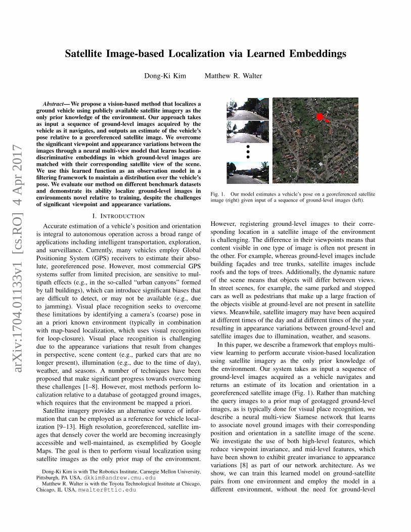
Fig. 1. Our model estimates a vehicle’s pose on a georeferenced satelliteimage (right) given input of a sequence of ground-level images (left).

However, registering ground-level images to their corre-sponding location in a satellite image of the environmentis challenging. The difference in their viewpoints means thatcontent visible in one type of image is often not present inthe other. For example, whereas ground-level images includebuilding facades and tree trunks, satellite images includeroofs and the tops of trees. Additionally, the dynamic natureof the scene means that objects will differ between views.In street scenes, for example, the same parked and stoppedcars as well as pedestrians that make up a large fraction ofthe objects visible at ground-level are not present in satelliteviews. Meanwhile, satellite imagery may have been acquiredat different times of the day and at different times of the year,resulting in appearance variations between ground-level andsatellite images due to illumination, weather, and seasons.

In this paper, we describe a framework that employs multi-view learning to perform accurate vision-based localizationusing satellite imagery as the only prior knowledge ofthe environment. Our system takes as input a sequence ofground-level images acquired as a vehicle navigates andreturns an estimate of its location and orientation in ageoreferenced satellite image (Fig. 1). Rather than matchingthe query images to a prior map of geotagged ground-levelimages, as is typically done for visual place recognition, wedescribe a neural multi-view Siamese network that learnsto associate novel ground images with their correspondingposition and orientation in a satellite image of the scene.We investigate the use of both high-level features, whichreduce viewpoint invariance, and mid-level features, whichhave been shown to exhibit greater invariance to appearancevariations [8] as part of our network architecture. As weshow, we can train this learned model on ground-satellitepairs from one environment and employ the model in adifferent environment, without the need for ground-level

arX

iv:1

704.

0113

3v1

[cs

.RO

] 4

Apr

201

7

images for fine-tuning. The framework uses outputs of thislearned matching function as observations in a particle filterthat maintains a distribution over the vehicle’s pose. Inthis way, our approach exploits the availability of satelliteimages to enable visual localization in a manner that isrobust to disparate viewpoints and appearance variations,without the need for a prior map of ground-level images. Weevaluate our method on the KITTI [14] and St. Lucia [15]datasets, and demonstrate the ability to transfer our learned,hierarchical multi-view model to novel environments andthereby localize the vehicle, despite the challenges of severeviewpoint variations and appearance changes.

II. RELATED WORK

The problem of estimating the location of a query groundimage is typically framed as one of finding the best matchagainst a database (i.e., map) of geotagged images. In gen-eral, existing approaches broadly fall into one of two classesdepending on the nature of the query and database images.

A. Single-View Localization

Single-view approaches assume access to referencedatabases that consist of geotagged images of the targetenvironment acquired from vantage points similar to thatof the query image (i.e., other ground-level images). Thesedatabases may come in the form of collections of Internet-based geotagged images, such as those available via photosharing websites [16–18] or Google Street View [19, 20],or maintained in maps of the environment (e.g., previouslyrecorded using GPS information or generated via SLAM) [1–4, 6–8, 21–24]. The primary challenges to visual placerecognition arise due to variations in viewpoint, variations inappearance that result from changes in environment structure,illumination, and seasons, as well as to perceptual aliasing.Much of the early work attempts to mitigate some of thesechallenges by using hand-crafted features that exhibit somerobustness to transformations in scale and rotation, as wellas to slight variations in illumination (e.g., SIFT [25] andSURF [26]), or a combination of visual and textual (i.e.,image tags) features [18]. Place recognition then follows asimage retrieval, i.e., image-to-image matching-based searchagainst the database [21, 27–29].

These techniques have proven effective at identifying thelocation of query images over impressively large areas [17].However, their reliance upon available reference imageslimits their use to regions with sufficient coverage and theiraccuracy depends on the spatial density of this coverage.Further, methods that use hand-crafted interest point-basedfeatures tend to fail when faced with significant viewpointand appearance variations, such as due to large illuminationchanges (e.g., matching a query image taken at night to adatabase image taken during the day) and seasonal changes(e.g., matching a query image with snow to one taken duringsummer). Recent attention in visual place recognition [6–8, 24, 30–34] has focused on designing algorithms thatexhibit improved invariance to the challenges of viewpointand appearance variations. Motivated by their state-of-the-art

performance on object detection and recognition tasks [35],a solution that has proven successful is to use deep con-volutional networks to learn suitable feature representations.Sunderhauf et al. [8] present a thorough analysis of the ro-bustness of different AlexNet [35] features to appearance andviewpoint variations. Based on these insights, Sunderhaufet al. [7] describe a framework that first detects candidatelandmarks in an image and then employs mid-level featuresfrom a convolutional neural network (AlexNet) to performplace recognition despite significant changes in appearanceand viewpoint. We also employ CNNs as a means of learningmid- and high-level features that exhibit improved robust-ness to viewpoint and appearance variations. Meanwhile,an alternative to single-view matching is to consider imagesequences when performing recognition [2–5, 36], wherebyimposing joint consistency reduces the likelihood of falsematches and improves robustness to appearance variations.

B. Cross-View Localization

Cross-view methods identify the location of a queryimage by matching against a database of images takenfrom disparate viewpoints. As in our case, this typicallyinvolves localizing ground-level images using a databaseof georeferenced satellite images [9–12, 12, 13, 37–39].Bansal et al. [10] describe a method that localizes street viewimages relative to a collection of geotagged oblique aerialand satellite images. Their method uses the combination ofsatellite and aerial images to extract building facades andtheir locations. Localization then follows by matching thesefacades against those in the query ground image. Meanwhile,Lin et al. [11] leverage the availability of land use attributesand propose a cross-view learning approach that learns thecorrespondence between hand-crafted interest-point featuresfrom ground-level images, overhead images, and land coverdata. Chu et al. [37] use a database of ground-level imagespaired with their corresponding satellite views to learn adictionary of color, edge, and neural features that they use forretrieval at test time. Unlike our method, which requires onlysatellite images of the target environment, both approachesassume access to geotagged ground-level images from thetest environment that are used for training and matching.

Viswanathan et al. [12] describe an algorithm that warps360◦ view ground images to obtain a projected top-downview that they then match to a grid of satellite locations usingtraditional hand-crafted features. As with our framework,they use the inferred poses as observations in a particle filter.The technique assumes that the ground-level and satelliteimages were acquired at similar times, and is thus not robustto the appearance variations that arise as a result of seasonalchanges. Viswanathan et al. [13] overcome this limitationby incorporating ground vs. non-ground pixel classificationsderived from available LIDAR scans, which improves ro-bustness to seasonal changes. As with their previous work,they also employ a Bayesian filter to maintain an estimateof the vehicle’s pose. In contrast, our method uses onlyan odometer and a non-panoramic, forward-facing camerawith a much narrower field-of-view. Rather than interest

Motion Update

Siamese Network

Odometry/IMU

Velocity &

Angular Rate

Satellite Imagery Query Ground Image

Weight Update

Feature Distance

Resampling

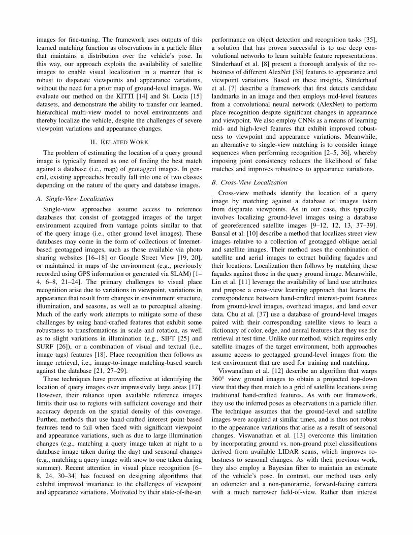
Fig. 2. Our method takes as input a stream of ground-level images andmaintains a distribution over the vehicle’s pose by comparing these imagesto a database of satellite images.

point features, we learn to separate location-discriminativefeature representations for ground-level and satellite views.These features include an encoding of the scene’s semanticproperties, serving a similar role to their ground labels.

Similar to our work is that of Lin et al. [38], who describea Siamese Network architecture that uses two CNNs to trans-form ground-level and aerial images into a common featurespace. Localizing a query ground image then correspondsto finding the closest georeferenced aerial image in thisspace. They train their network on a database of ground-aerial pairs and demonstrate the ability to localize test imagesfrom environments not encountered during training. Unlikeour method, they match against 45◦ aerial images, whichshare more content with ground-level images (e.g., buildingfacades) than do satellite views. Additionally, whereas theirSiamese network extends AlexNet [35] by using only thesecond-to-last connected layer (fc7) as the high-level feature,our network adapts VGG-16 [40] with modifications thatconsider the use of both mid-level and high-level featuresto improve robustness to changes in appearance.

III. PROPOSED APPROACH

Our visual localization framework (Fig. 2) takes as inputa stream of ground-level images Itg = {. . . , It−2, It−1, It}from a camera mounted to the vehicle and proprioceptivemeasurements of the vehicle’s motion (e.g., from an odome-ter and IMU), and outputs a distribution over the vehicle’spose xt relative to a database of georeferenced satelliteimages Is, which constitutes the only prior knowledge ofthe environment. The method consists of a Siamese networkthat learns feature embeddings suitable to matching ground-level imagery with their corresponding satellite view. Thesematches then serve as noisy observations of the vehicle’sposition and orientation that are then incorporated into aparticle filter to maintain a distribution over its pose as itnavigates. Next, we describe these components in detail.

A. Siamese Network

Our method matches a query ground-level image to itscorresponding satellite view using a Siamese network [41],which has proven effective at different multi-view learningtasks [42]. Siamese networks consist of two convolutional

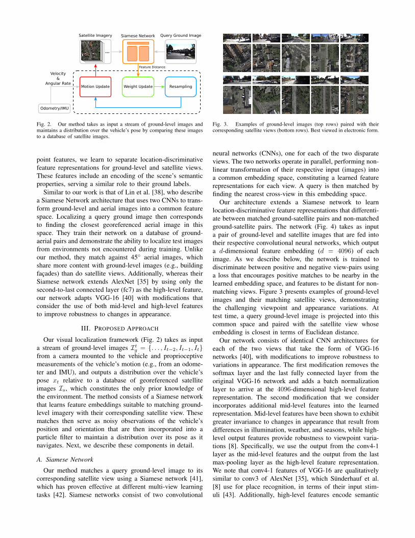
Fig. 3. Examples of ground-level images (top rows) paired with theircorresponding satellite views (bottom rows). Best viewed in electronic form.

neural networks (CNNs), one for each of the two disparateviews. The two networks operate in parallel, performing non-linear transformation of their respective input (images) intoa common embedding space, constituting a learned featurerepresentations for each view. A query is then matched byfinding the nearest cross-view in this embedding space.

Our architecture extends a Siamese network to learnlocation-discriminative feature representations that differenti-ate between matched ground-satellite pairs and non-matchedground-satellite pairs. The network (Fig. 4) takes as inputa pair of ground-level and satellite images that are fed intotheir respective convolutional neural networks, which outputa d-dimensional feature embedding (d = 4096) of eachimage. As we describe below, the network is trained todiscriminate between positive and negative view-pairs usinga loss that encourages positive matches to be nearby in thelearned embedding space, and features to be distant for non-matching views. Figure 3 presents examples of ground-levelimages and their matching satellite views, demonstratingthe challenging viewpoint and appearance variations. Attest time, a query ground-level image is projected into thiscommon space and paired with the satellite view whoseembedding is closest in terms of Euclidean distance.

Our network consists of identical CNN architectures foreach of the two views that take the form of VGG-16networks [40], with modifications to improve robustness tovariations in appearance. The first modification removes thesoftmax layer and the last fully connected layer from theoriginal VGG-16 network and adds a batch normalizationlayer to arrive at the 4096-dimensional high-level featurerepresentation. The second modification that we considerincorporates additional mid-level features into the learnedrepresentation. Mid-level features have been shown to exhibitgreater invariance to changes in appearance that result fromdifferences in illumination, weather, and seasons, while high-level output features provide robustness to viewpoint varia-tions [8]. Specifically, we use the output from the conv4-1layer as the mid-level features and the output from the lastmax-pooling layer as the high-level feature representation.We note that conv4-1 features of VGG-16 are qualitativelysimilar to conv3 of AlexNet [35], which Sunderhauf et al.[8] use for place recognition, in terms of their input stim-uli [43]. Additionally, high-level features encode semantic

Satellite Image

Ground-level Image

Conv + ReLU

Max Pooling

Conv 4-1

Average Pooling

Loss Layer

Fully-Connected

Merge Layer

224x224x3

FeatureDistance

224x224x64

112x112x12856x56x256

14x14x512

28x28x512

28x28x512

7x7x512

7x7x512

4096

7x7x512

4096

224x224x64

112x112x12856x56x256

14x14x512

28x28x512

28x28x512

7x7x512

7x7x512

4096

7x7x512

4096

224x224x3

Fig. 4. A visualization of our network architecture that consists of two independent CNNs that take as input ground-level and satellite images. Each CNNis an adaptation of VGG-16 CNNs in which mid-level conv4-1 features are downsampled and combined with the output of the last max-pooling layer asthe high-level features via summation. The resulting outputs are then used as a measure of distance between ground-level and satellite views.

information, which is particularly useful for categorizingscenes, while mid-level features tend to be better suited todiscriminating between instances of particular scenes. In thisway, the two feature representations are complementary. Wedownsample the conv4-1 mid-level features to match the sizeof the output from the last max-pooling layer using average-pooling, and combine the two via summation.1 We evaluatethe effect of combining these features in Section IV.

We train our network so as to learn nonlinear transfor-mations of input pairs that bring embeddings of match-ing ground-level and satellite images closer together, whiledriving the embeddings associated with non-matching pairsfarther apart. To that end, we use a contrastive loss [44]

L(Ig, Is, `) = `d(Ig, Is)2+(1−`)max(m−d(Ig, Is), 0)2 (1)

to define the loss between a pair of ground-level Ig andsatellite Is images, where ` is a binary-valued correspon-dence variable that indicates whether the pair match (` = 1),d(Ig, Is) is the Euclidean distance between the image featureembeddings, and m > 0 is a margin for non-matched pairs.

In the case of matching pairs of ground-level and satelliteimages (` = 1), the loss encourages the network to learnfeature representations that are nearby in the common em-bedding space. In the case of non-matching pairs (` = 0),the contrastive loss penalizes the network for transformingthe images into features that are separated by a distanceless than the margin m. In this way, training will tend topull matching ground-level and satellite image pairs closertogether, while keeping non-matching images at least a radiusm apart, which provides a form of regularization againsttrivial solutions [44].

The ground-level and satellite CNN networks can sharemodel parameters or be trained separately. We chose to trainthe networks with separate parameters for each CNN, but

1We explored other methods for combining the two representationsincluding concatenation on a validation set, but found summation to yieldthe best performance.

note that previous efforts found little difference with the ad-dition of parameter sharing in similar Siamese networks [38].

B. Particle Filter

The learned distance function modeled by the convo-lutional neural network provides a good measure of thesimilarity between ground-level imagery and the database ofsatellite views. As a result of perceptual aliasing, however,it is possible that the match that minimizes the distancebetween the learned features does not correspond to thecorrect location. In order to mitigate the effect of this noise,we maintain a distribution over the vehicle’s pose as itnavigates the environment

p(xt|ut, zt), (2)

where xt is the pose of the vehicle and ut = {u0, u1, . . . , ut}denotes the history of proprioceptive measurements (i.e.,forward velocity and angular rate). The term zt ={z0, z1, . . . , zt} corresponds to the history of image-basedobservations, each consisting of the distance d(Ig, Is) in thecommon embedding space between the transformed ground-level image It and the satellite image Is ∈ Is with a positionand orientation specified by xt.2

The posterior over the vehicle’s pose tends to be multi-modal. Consequently, we represent the distribution using aset of weighted particles

Pt ={P

(1)t , P

(2)t , . . . , P

(n)t

}, (3)

where each particle P (i)t = {x(i)t , w

(i)t } includes a sampled

vehicle pose x(i)t and the particle’s importance weight w(i)t .

We maintain the posterior distribution as new odometryand ground-level images arrive using a particle filter. Figure 2provides a visual overview of this process. Given the poste-rior distribution p(xt−1|ut−1, zt−1) over the vehicle’s pose attime t−1, we first compute the prior distribution over xt by

2In the case of forward-facing ground-level cameras, the location associ-ated with the center of the satellite image is in front of the vehicle.

sampling from the motion model prior p(xt|xt−1, ut, zt−1),

which we model as Gaussian.After proposing a new set of particles, we update their

weights to according to the ratio between the target (poste-rior) and proposal (prior) distributions

w(i)t = p(zt|xt, ut, zt−1) · w(i)

t−1, (4)

where w(i)t denotes the unnormalized weight at time t.

We use the output of the Siamese network to define themeasurement likelihood as an exponential distribution

p(zt|xt, ut, zt−1) = αe−αd(It,Is), (5)

where d(It, Is) is the Euclidean distance between the CNNembeddings of the current ground-level image It and thesatellite image Is corresponding to pose xt, and α is a tunedparameter.

After having calculated and normalized the new impor-tance weights, we periodically perform resampling in orderto discourage particle depletion based on the effective num-ber of particles

Neff =1

N∑i=1

w(i)t

2(6)

Specifically, we use systematic resampling [45] when theeffective number of particles Neff drops below a threshold.

IV. RESULTS

We evaluate our model through a series of experimentsconducted on two benchmark, publicly available visual lo-calization datasets. We consider two versions of our architec-ture: Ours-Mid uses both mid- and high-level features, whileOurs uses only high-level features. The experiments analyzethe ability of our framework to generalize to different test en-vironments and to mitigate appearance variations that resultfrom changes in semantic scene content and illumination.

A. Experimental Setup

Our evaluation involves training our network on pairsof ground-level and satellite images from a portion of theKITTI [14] dataset, and testing our method on a differentregion from KITTI and the St. Lucia dataset [15].

1) Baselines: We compare the performance of our modelagainst two baselines that consider both hand-crafted andlearned feature representations. The first baseline (SIFT)extracts SIFT features [25] from each ground-level andsatellite image and computes the distance between a queryground-level image and the extracted satellite image as theaverage distance associated with the best-matching features.The second baseline (AlexNet-Places) employs a Siamesenetwork comprised of two AlexNet deep convolutional net-works [35] trained on the Places dataset [46]. We use the4096 dimensional output of the fc7 layer as the embeddingwhen computing the distance used in the measurementupdate step of the particle filter.

2) Training Details: Our training data is drawn from theKITTI dataset, collected from a moving vehicle in Karlsruhe,Germany during the daytime in the months of Septemberand October. The dataset consists of sequences that spanvariations of city, residential, and road scenes. Of these, werandomly sample 18 sequences from the city, residential, androad categories as the training set, and 5 from the city androad categories as the validation set, resulting in 14.8k and1.3k ground-level images, respectively.

For each ground-level image in the training and validationsets, we sample a 270 × 400 (53m × 78m) satellite imageat a position 5.0m in front of the camera with the long-axisoriented in the direction of the camera. We also include arandomly sampled set of non-matching satellite images. Wedefine a pair of ground-level and satellite images (Ig, Is)to be a match (` = 1) if their distance is within 4m andtheir orientation within 30 degrees. We consider non-matches(` = 0) as those that are more than 80m apart.3 The resultingtraining set then consists of 538k pairs (53k positive pairs and485k negative pairs). Figure 3 presents samples drawn fromthe set of positive pairs, which demonstrate the challenge ofmatching these disparate views.

We trained our models from scratch4 using the contrastiveloss (Eqn. 1) with a margin of m = 80 (tuned on the valida-tion set) using Adam [47] on an Nvidia Titan X. Meanwhile,we used the validation set to tune hyper-parameters includingthe early stopping criterion, as well as to explore differentvariations of our network architecture, including alternativemethods for combining mid- and high-level features and theuse of max-pooling instead of average-pooling.

3) Particle Filter Implementation: In each experiment,we used N = 5000 particles representing samples of thevehicle’s position and orientation. We assumed that thevehicle’s initial pose was unknown (i.e., the kidnapped robotsetting), and biased the initialization of each filter such thatsamples were more likely to be drawn on roadways. Particleswere resampled using Neff = 0.8N (tuned on a validationset). We determine a filter to have converged when thestandard deviation of the estimates is less than 10m.

B. Experimental Results

We evaluate two versions of our method against thedifferent baselines with regards to the effects of appearancevariations due to changes in viewpoint, location, scene con-tent, and illumination both between training and test as wellas between the reference satellite and ground-level imagery.We analyze the performance in terms of precision-recall aswell as retrieval. We then investigate the accuracy with whichthe particle filter is able to localize the vehicle as it navigates.

1) KITTI Experiment: We evaluate our method on KITTIusing two residential sequences (KITTI-Test-A and KITTI-Test-B) as test sets. We note that there is no environmentoverlap between these sequences and those used for training

3These parameters were tuned on the validation set.4We also tried fine-tuning from models pre-trained on ImageNet and

Places and found the results to be comparable.

0 0.1 0.2 0.3 0.4 0.5 0.6 0.7 0.8 0.9 1Recall

0

0.1

0.2

0.3

0.4

0.5

0.6

0.7

0.8

0.9

1Pr

ecis

ion

SIFT (0.11854)ALEXNET-PLACES (0.13717)OURS (0.16905)OURS-MID (0.33426)

(a) Precision-Recall

0 10 20 30 40 50 60 70 80 90 100Top Percentage of Satellite Images

0

0.1

0.2

0.3

0.4

0.5

0.6

0.7

0.8

0.9

1

Frac

tion

of G

roun

d-Le

vel I

mag

es

SIFTALEXNET-PLACESOURSOURS-MID

(b) Retrieval Accuracy

Fig. 5. Results on the KITTI test set including (a) precision-recall curveswith the average precision values in parentheses and (b) retrieval accuracy.

or validation. The georeferenced satellite maps for KITTI-Test-A is 0.80 km × 1.10 km and 0.53 km × 0.70 km forKITTI-Test-B.

Figure 5(a) compares the precision-recall curve of ourmodels against the two baseline for the two KITTI testsequences. The plot additionally includes the average pre-cision for each model. The plot shows that Ours-Mid is themost effective at matching ground-level images with theircorresponding satellite views. The use of a contrastive lossas a means of encouraging our network to bring positivepairs closer together facilitates accurate matching. Compar-ing against the performance of Ours demonstrates that theincorporation of mid-level features helps to mitigate theeffects of appearance variations. Meanwhile, the AlexNet-Places baseline that uses the output of AlexNet trained onPlaces as the learned feature embeddings outperforms theSIFT baseline that relies upon hand-designed SIFT featuresto identify correspondences.

As another measure of the discriminative ability of ournetwork architecture, we consider the frequency with whichthe correct satellite view is in the top-X% matches for agiven ground-level image according to the feature embeddingdistance. Figure 5(b) plots the fraction of query ground-level images for which the corresponding satellite view isfound in the top-X% of the satellite images. In the caseof both Ours-Mid and Ours, the correct satellite view is inthe top 10% for more than 50% of the ground-level images.When we increase the size of the candidate set, our method

TABLE IFINAL MEAN POSITION ERROR AND STANDARD DEVIATION (IN METERS)

KITTI-Test-A KITTI-Test-B St-Lucia

SIFT 656.70 (244.29) 243.08 (79.63) 554.35 (17.26)AlexNet-Places 177.82 (25.68) 59.95 (38.99) 77.15 (52.61)Ours 8.41 (5.56) 7.93 (2.14) 26.38 (5.63)Ours-Mid 7.69 (5.14) 4.65 (2.77) 35.81 (7.54)

yields a slight increase in performance (around 4%). TheAlexNet-Places baseline performs slightly worse, while allthree significantly outperform the SIFT baseline, which isessentially equivalent to chance.

Next, we evaluate our method’s ability to estimate thevehicle’s pose as it navigates the environment by usingthe distance between the learned feature representations asobservations in the particle filter. In Table I, we reportthe quantitative results for each of the two KITTI testenvironments. Note that the final position mean error andstandard deviation is measured at the last ground-level imagesequence using all of the particles. Figure 6 depicts theconverged particle filter estimate of the vehicle’s positionusing Ours-Mid compared to the ground-truth position. Forboth KITTI-Test-A and KITTI-Test-B, the filter that usesOurs-Mid has smaller average position errors, compared tothe one that uses Ours. Using Ours-Mid, the filter convergedat 55.62 s and 62.25 s for KITTI-Test-A and KITTI-Test-B,respectively, and using Ours, the filter converged at 64.67 sand 70.15 s for KITTI-Test-A and KITTI-Test-B, respec-tively. Meanwhile, the SIFT baseline failed to converge withlarge average errors for both KITTI-Test-A and KITTI-Test-B. The AlexNet-Places baseline faired better, but the filteralso did not converge for either of the test sets. The resultssupport the argument that our method’s ability to learn mid-and high-level feature representations with a loss that bringsground-level image embeddings closer to their correspondingsatellite representation results in measurements that are ableto distinguish between correct and incorrect matches.

2) St. Lucia Experiment: Next, we consider the St. Luciadataset [15] as a means of evaluating the method’s ability togeneralize the model trained on KITTI to new environmentswith differing semantic content. The dataset was collectedduring August from a car driving through a suburb of Bris-bane, Australia at different times during a single day and overdifferent days during a two week period. We use the datasetcollected on August 21 at 12:10 as the validation set and thedataset collected on August 19 at 14:10 as the test set. Thetwo exhibit slight variations in viewpoint due to differencesin the vehicle’s route. More pronounced appearance vari-ations result from illumination changes and non-stationaryobjects in the environment (e.g., cars and pedestrians). Notethat the dataset does not include the vehicle’s velocity orangular rate. As done elsewhere [31] we simulate visualodometry by interpolating the GPS differential, which isprone to significant noise and is thereby representative ofthe quality of data that visual odometry would yield. Thegeoreferenced satellite map is 1.8 km ×1.2 km.

N

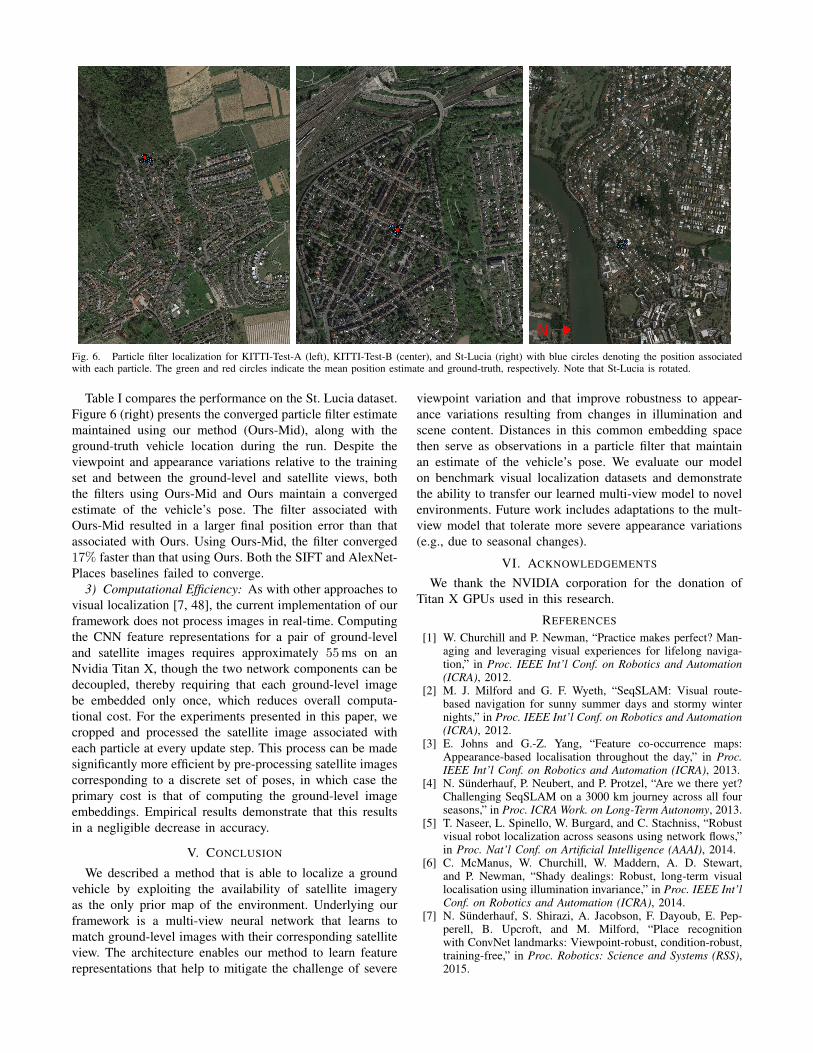
Fig. 6. Particle filter localization for KITTI-Test-A (left), KITTI-Test-B (center), and St-Lucia (right) with blue circles denoting the position associatedwith each particle. The green and red circles indicate the mean position estimate and ground-truth, respectively. Note that St-Lucia is rotated.

Table I compares the performance on the St. Lucia dataset.Figure 6 (right) presents the converged particle filter estimatemaintained using our method (Ours-Mid), along with theground-truth vehicle location during the run. Despite theviewpoint and appearance variations relative to the trainingset and between the ground-level and satellite views, boththe filters using Ours-Mid and Ours maintain a convergedestimate of the vehicle’s pose. The filter associated withOurs-Mid resulted in a larger final position error than thatassociated with Ours. Using Ours-Mid, the filter converged17% faster than that using Ours. Both the SIFT and AlexNet-Places baselines failed to converge.

3) Computational Efficiency: As with other approaches tovisual localization [7, 48], the current implementation of ourframework does not process images in real-time. Computingthe CNN feature representations for a pair of ground-leveland satellite images requires approximately 55ms on anNvidia Titan X, though the two network components can bedecoupled, thereby requiring that each ground-level imagebe embedded only once, which reduces overall computa-tional cost. For the experiments presented in this paper, wecropped and processed the satellite image associated witheach particle at every update step. This process can be madesignificantly more efficient by pre-processing satellite imagescorresponding to a discrete set of poses, in which case theprimary cost is that of computing the ground-level imageembeddings. Empirical results demonstrate that this resultsin a negligible decrease in accuracy.

V. CONCLUSION

We described a method that is able to localize a groundvehicle by exploiting the availability of satellite imageryas the only prior map of the environment. Underlying ourframework is a multi-view neural network that learns tomatch ground-level images with their corresponding satelliteview. The architecture enables our method to learn featurerepresentations that help to mitigate the challenge of severe

viewpoint variation and that improve robustness to appear-ance variations resulting from changes in illumination andscene content. Distances in this common embedding spacethen serve as observations in a particle filter that maintainan estimate of the vehicle’s pose. We evaluate our modelon benchmark visual localization datasets and demonstratethe ability to transfer our learned multi-view model to novelenvironments. Future work includes adaptations to the mult-view model that tolerate more severe appearance variations(e.g., due to seasonal changes).

VI. ACKNOWLEDGEMENTS

We thank the NVIDIA corporation for the donation ofTitan X GPUs used in this research.

REFERENCES

[1] W. Churchill and P. Newman, “Practice makes perfect? Man-aging and leveraging visual experiences for lifelong naviga-tion,” in Proc. IEEE Int’l Conf. on Robotics and Automation(ICRA), 2012.

[2] M. J. Milford and G. F. Wyeth, “SeqSLAM: Visual route-based navigation for sunny summer days and stormy winternights,” in Proc. IEEE Int’l Conf. on Robotics and Automation(ICRA), 2012.

[3] E. Johns and G.-Z. Yang, “Feature co-occurrence maps:Appearance-based localisation throughout the day,” in Proc.IEEE Int’l Conf. on Robotics and Automation (ICRA), 2013.

[4] N. Sunderhauf, P. Neubert, and P. Protzel, “Are we there yet?Challenging SeqSLAM on a 3000 km journey across all fourseasons,” in Proc. ICRA Work. on Long-Term Autonomy, 2013.

[5] T. Naseer, L. Spinello, W. Burgard, and C. Stachniss, “Robustvisual robot localization across seasons using network flows,”in Proc. Nat’l Conf. on Artificial Intelligence (AAAI), 2014.

[6] C. McManus, W. Churchill, W. Maddern, A. D. Stewart,and P. Newman, “Shady dealings: Robust, long-term visuallocalisation using illumination invariance,” in Proc. IEEE Int’lConf. on Robotics and Automation (ICRA), 2014.

[7] N. Sunderhauf, S. Shirazi, A. Jacobson, F. Dayoub, E. Pep-perell, B. Upcroft, and M. Milford, “Place recognitionwith ConvNet landmarks: Viewpoint-robust, condition-robust,training-free,” in Proc. Robotics: Science and Systems (RSS),2015.

[8] N. Sunderhauf, F. Dayoub, S. Shirazi, B. Upcroft, and M. Mil-ford, “On the performance of ConvNet features for placerecognition,” in Proc. IEEE/RSJ Int’l Conf. on IntelligentRobots and Systems (IROS), 2015.

[9] N. Jacobs, S. Satkin, N. Roman, and R. Speyer, “Geolocatingstatic cameras,” in Proc. Int’l Conf. on Computer Vision(ICCV), 2007.

[10] M. Bansal, H. S. Sawhney, H. Cheng, and K. Daniilidis, “Geo-localization of street views with aerial image databases,” inProc. ACM Int’l Conf. on Multimedia (MM), 2011.

[11] T.-Y. Lin, S. Belongie, and J. Hays, “Cross-view imagegeolocalization,” in Proc. IEEE Conf. on Computer Vision andPattern Recognition (CVPR), 2013.

[12] A. Viswanathan, B. R. Pires, and D. Huber, “Vision basedrobot localization by ground to satellite matching in GPS-denied situations,” in Proc. IEEE/RSJ Int’l Conf. on IntelligentRobots and Systems (IROS), 2014.

[13] ——, “Vision-based robot localization across seasons and inremote locations,” in Proc. IEEE Int’l Conf. on Robotics andAutomation (ICRA), 2016.

[14] A. Geiger, P. Lenz, C. Stiller, and R. Urtasun, “Vision meetsrobotics: The KITTI dataset,” Int’l J. of Robotics Research,vol. 32, no. 11, 2013.

[15] M. Warren, D. McKinnon, H. He, and B. Upcroft, “Unaidedstereo vision based pose estimation,” in Proc. AustralasianConf. on Robotics and Automation, 2010.

[16] W. Zhang and J. Kosecka, “Image based localization in urbanenvironments,” in Proc. Int’l Symp. on 3D Data Processing,Visualization, and Transmission, 2006.

[17] J. Hays and A. A. Efros, “IM2GPS: Estimating geographicinformation from a single image,” in Proc. IEEE Conf. onComputer Vision and Pattern Recognition (CVPR), 2008.

[18] D. J. Crandall, L. Backstrom, D. Huttenlocher, and J. Klein-berg, “Mapping the world’s photos,” in Proc. Int’l World WideWeb Conf. (WWW), 2009.

[19] A. R. Zamir and M. Shah, “Accurate image localization basedon Google Maps Street View,” in Proc. European Conf. onComputer Vision (ECCV), 2010.

[20] A. L. Majdik, Y. Albers-Schoenberg, and D. Scaramuzza,“MAV urban localization from Google Street View data,” inProc. IEEE/RSJ Int’l Conf. on Intelligent Robots and Systems(IROS), 2013.

[21] G. Schindler, M. Brown, and R. Szeliski, “City-scale locationrecognition,” in Proc. IEEE Conf. on Computer Vision andPattern Recognition (CVPR), 2007.

[22] M. Cummins and P. Newman, “FAB-MAP: Probabilistic local-ization and mapping in the space of appearance,” InternationalJournal of Robotics Research, vol. 27, no. 6, 2008.

[23] D. M. Chen, G. Baatz, K. Koser, S. S. Tsai, R. Vedantham,T. Pylvanainen, K. Roimela, X. Chen, J. Bach, M. Pollefeys,B. Girod, and R. Grzeszczuk, “City-scale landmark identifi-cation on mobile devices,” in Proc. IEEE Conf. on ComputerVision and Pattern Recognition (CVPR), 2011.

[24] H. Badino, D. Huber, and T. Kanade, “Real-time topometriclocalization,” in Proc. IEEE Int’l Conf. on Robotics andAutomation (ICRA), 2012.

[25] D. G. Lowe, “Distinctive image features from scale-invariantkeypoints,” Int’l J. on Computer Vision, vol. 60, no. 2, 2004.

[26] H. Bay, T. Tuytelaars, and L. Van Gool, “Surf: Speeded uprobust features,” in Proc. European Conf. on Computer Vision(ECCV), 2006.

[27] J. Wolf, W. Burgard, and H. Burkhardt, “Robust vision- basedlocalization by combining an image-retrieval system withmonte carlo localization,” Trans. on Robotics, vol. 21, no. 2,2005.

[28] F. Li and J. Kosecka, “Probabilistic location recognition usingreduced feature set,” in Proc. IEEE Int’l Conf. on Robotics andAutomation (ICRA), 2006.

[29] D. Filliat, “A visual bag of words method for interactivequalitative localization and mapping,” in Proc. IEEE Int’lConf. on Robotics and Automation (ICRA), 2007.

[30] C. Valgren and A. J. Lilienthal, “SIFT, SURF and seasons:Long-term outdoor localization using local features,” in Proc.European Conf. on Mobile Robotics (ECMR), 2007.

[31] A. J. Glover, W. P. Maddern, M. J. Milford, and G. F.Wyeth, “FAB-MAP + RatSLAM: Appearance-based SLAMfor multiple times of day,” in Proc. IEEE Int’l Conf. onRobotics and Automation (ICRA), 2010.

[32] P. Neubert, N. Sunderhauf, and P. Protzel, “Appearance changeprediction for long-term navigation across seasons,” in Proc.European Conf. on Mobile Robotics (ECMR), 2013.

[33] W. Maddern, A. Stewart, C. McManus, B. Upcroft,W. Churchill, and P. Newman, “Transforming morning toafternoon using linear regression techniques,” in Proc. IEEEInt’l Conf. on Robotics and Automation (ICRA), 2014.

[34] S. M. Lowry, M. J. Milford, and G. F. Wyeth, “Transformingmorning to afternoon using linear regression techniques,” inProc. IEEE Int’l Conf. on Robotics and Automation (ICRA),2014.

[35] A. Krizhevsky, I. Sutskever, and G. E. Hinton, “ImageNetclassification with deep convolutional neural networks,” inAdv. Neural Information Processing Systems (NIPS), 2012.

[36] O. Koch, M. R. Walter, A. Huang, and S. Teller, “Groundrobot navigation using uncalibrated cameras,” in Proc. IEEEInt’l Conf. on Robotics and Automation (ICRA), 2010.

[37] H. Chu, H. Mei, M. Bansal, and M. R. Walter, “Accu-rate vision-based vehicle localization using satellite imagery,”arXiv:1510.09171, 2015.

[38] T.-Y. Lin, Y. Cui, S. Belongie, and J. Hays, “Learning deeprepresentations for ground-to-aerial geolocalization,” in Proc.IEEE Conf. on Computer Vision and Pattern Recognition(CVPR), 2015.

[39] S. Workman, R. Souvenir, and N. Jacobs, “Wide-area imagegeolocalization with aerial reference imagery,” in Proc. Int’lConf. on Computer Vision (ICCV), 2015.

[40] K. Simonyan and A. Zisserman, “Very deep convolutionalnetworks for large-scale image recognition,” in Proc. Int’lConf. on Learning Representations (ICLR), 2015.

[41] S. Chopra, R. Hadsell, and Y. LeCun, “Learning a similaritymetric discriminatively, with application to face verification,”in Proc. IEEE Conf. on Computer Vision and Pattern Recog-nition (CVPR), 2005.

[42] Y. Taigman, M. Yang, M. Ranzato, and L. Wolf, “DeepFace:Closing the gap to human-level peformance in face verifica-tion,” in Proc. IEEE Conf. on Computer Vision and PatternRecognition (CVPR), 2014.

[43] M. D. Zeiler and R. Fergus, “Visualizing and understandingconvolutional networks,” in Proc. European Conf. on Com-puter Vision (ECCV), 2014.

[44] R. Hadsell, S. Chopra, and Y. LeCun, “Dimensionality reduc-tion by learning an invariant mapping,” in Proc. IEEE Conf.on Computer Vision and Pattern Recognition (CVPR), 2006.

[45] J. Carpenter, P. Clifford, and P. Fearnhead, “Improved particlefilter for nonlinear problems,” in Proc. Radar, Sonar, andNavigation, vol. 146, no. 1, 1999.

[46] B. Zhou, A. Lapedriza, J. X. nd A. Torralba, and A. Oliva,“Learning deep features for scene recognition using the Placesdatabase,” in Adv. Neural Information Processing Systems(NIPS), 2014.

[47] D. Kingma and J. Ba, “Adam: A method for stochastic op-timization,” in Proc. Int’l Conf. on Learning Representations(ICLR), 2015.

[48] C. McManus, B. Upcroft, and P. Newman, “Scene signatures:Localised and point-less features for localisation,” in Proc.Robotics: Science and Systems (RSS), 2014.