domain decomposition algorithms for time …...domain decomposition algorithms for time-harmonic...

Mathematical Modelling and Numerical Analysis ESAIM: M2AN

Modelisation Mathematique et Analyse Numerique Vol. 35, No 4, 2001, pp. 825–848

DOMAIN DECOMPOSITION ALGORITHMS FOR TIME-HARMONICMAXWELL EQUATIONS WITH DAMPING

Ana Alonso Rodriguez1

and Alberto Valli2

Abstract. Three non-overlapping domain decomposition methods are proposed for the numericalapproximation of time-harmonic Maxwell equations with damping (i.e., in a conductor). For eachmethod convergence is proved and, for the discrete problem, the rate of convergence of the iterativealgorithm is shown to be independent of the number of degrees of freedom.

Mathematics Subject Classification. 65N55, 65N30.

Received: March 23, 2000. Revised: March 30, 2001.

1. Introduction

The time-harmonic Maxwell equations are derived from the complete Maxwell equations assuming thatboth the electric field E and the magnetic field H are of the form E(t,x) = Re[E(x) exp(iωt)], H(t,x) =Re[H(x) exp(iωt)], where ω 6= 0 is a given angular frequency. Let Ω ⊂ R3 be a bounded Lipschitz polyhedronwith unit outward normal n. Let ε(x), µ(x) and σ(x) denote respectively the dielectric constant, the magneticpermeability and the conductivity of the medium. The time-harmonic Maxwell equations reads:

(iωε+ σ)E− rot H = J in ΩiωµH + rot E = 0 in Ω, (1)

where J = J(x) is a known function specifying the applied current density. (See [9] for a complete presentationof time-harmonic Maxwell equations.)

In the general case of anisotropic inhomogeneous media the coefficients ε, µ and σ are 3× 3 symmetric realmatrices with entries in L∞(Ω). The matrices ε and µ are assumed to be uniformly positive definite in Ω. (Amatrix ζ(x) is uniformly positive definite in Ω if there exists a constant ζ∗ > 0 such that

∑3l,m=1 ζl,m(x)ξlξm ≥

ζ∗|ξξξ|2 for almost all x ∈ Ω and for all ξξξ ∈ C3.) The conductivity σ is an uniformly positive definite matrix in aconductor and it is equal to 0 in an insulator.

As µ is non-singular we may eliminate the magnetic field H in (1) to obtain

rot (µ−1rot E)− ω2εE + iωσE = iωJ. (2)

Keywords and phrases. Time-harmonic Maxwell equations, domain decomposition methods, edge finite elements.

1 Dipartimento di Matematica, Universita degli Studi di Milano, via Saldini 50, 20133 Milano, Italy.e-mail: [email protected], [email protected] Dipartimento di Matematica, Universita degli Studi di Trento, 38050 Povo (Trento), Italy. e-mail: [email protected]

c© EDP Sciences, SMAI 2001

826 A. ALONSO RODRIGUEZ AND A. VALLI

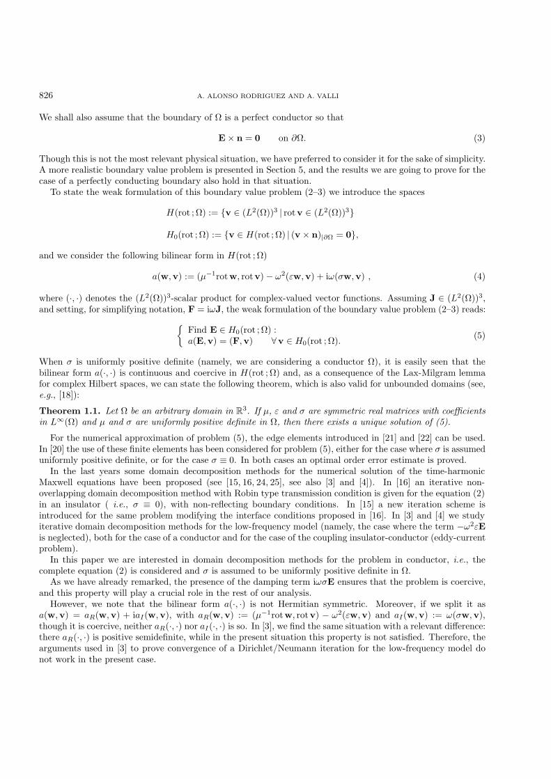
We shall also assume that the boundary of Ω is a perfect conductor so that

E× n = 0 on ∂Ω. (3)

Though this is not the most relevant physical situation, we have preferred to consider it for the sake of simplicity.A more realistic boundary value problem is presented in Section 5, and the results we are going to prove for thecase of a perfectly conducting boundary also hold in that situation.

To state the weak formulation of this boundary value problem (2–3) we introduce the spaces

H(rot ; Ω) := v ∈ (L2(Ω))3 | rot v ∈ (L2(Ω))3

H0(rot ; Ω) := v ∈ H(rot ; Ω) | (v× n)|∂Ω = 0,

and we consider the following bilinear form in H(rot ; Ω)

a(w,v) := (µ−1rot w, rot v) − ω2(εw,v) + iω(σw,v) , (4)

where (·, ·) denotes the (L2(Ω))3-scalar product for complex-valued vector functions. Assuming J ∈ (L2(Ω))3,and setting, for simplifying notation, F = iωJ, the weak formulation of the boundary value problem (2–3) reads:

Find E ∈ H0(rot ; Ω) :a(E,v) = (F,v) ∀v ∈ H0(rot ; Ω). (5)

When σ is uniformly positive definite (namely, we are considering a conductor Ω), it is easily seen that thebilinear form a(·, ·) is continuous and coercive in H(rot ; Ω) and, as a consequence of the Lax-Milgram lemmafor complex Hilbert spaces, we can state the following theorem, which is also valid for unbounded domains (see,e.g., [18]):

Theorem 1.1. Let Ω be an arbitrary domain in R3. If µ, ε and σ are symmetric real matrices with coefficientsin L∞(Ω) and µ and σ are uniformly positive definite in Ω, then there exists a unique solution of (5).

For the numerical approximation of problem (5), the edge elements introduced in [21] and [22] can be used.In [20] the use of these finite elements has been considered for problem (5), either for the case where σ is assumeduniformly positive definite, or for the case σ ≡ 0. In both cases an optimal order error estimate is proved.

In the last years some domain decomposition methods for the numerical solution of the time-harmonicMaxwell equations have been proposed (see [15, 16, 24, 25], see also [3] and [4]). In [16] an iterative non-overlapping domain decomposition method with Robin type transmission condition is given for the equation (2)in an insulator ( i.e., σ ≡ 0), with non-reflecting boundary conditions. In [15] a new iteration scheme isintroduced for the same problem modifying the interface conditions proposed in [16]. In [3] and [4] we studyiterative domain decomposition methods for the low-frequency model (namely, the case where the term −ω2εEis neglected), both for the case of a conductor and for the case of the coupling insulator-conductor (eddy-currentproblem).

In this paper we are interested in domain decomposition methods for the problem in conductor, i.e., thecomplete equation (2) is considered and σ is assumed to be uniformly positive definite in Ω.

As we have already remarked, the presence of the damping term iωσE ensures that the problem is coercive,and this property will play a crucial role in the rest of our analysis.

However, we note that the bilinear form a(·, ·) is not Hermitian symmetric. Moreover, if we split it asa(w,v) = aR(w,v) + iaI(w,v), with aR(w,v) := (µ−1rot w, rot v) − ω2(εw,v) and aI(w,v) := ω(σw,v),though it is coercive, neither aR(·, ·) nor aI(·, ·) is so. In [3], we find the same situation with a relevant difference:there aR(·, ·) is positive semidefinite, while in the present situation this property is not satisfied. Therefore, thearguments used in [3] to prove convergence of a Dirichlet/Neumann iteration for the low-frequency model donot work in the present case.

DOMAIN DECOMPOSITION ALGORITHMS FOR TIME-HARMONIC MAXWELL EQUATIONS 827

We are going to see in the sequel that the main difficulty arises from the fact that the bilinear form a(·, ·)is not Hermitian symmetric. We recall that, for non-overlapping domain decomposition methods, an analysisof convergence (also concerning the independence of the convergence rate of the mesh size) is based in generalon the assumption that the problem is Hermitian symmetric (indeed, most often on the assumption that theproblem is real and symmetric).

In this paper we aim to present a complete convergence analysis when the problem is complex and not Hermit-ian symmetric. More precisely, we introduce and analyse two families of non-overlapping domain decompositionmethods: γ-Dirichlet/Robin methods and γ-Robin/Robin methods. These domain decomposition proceduresare both related to algorithms used for advection–diffusion equations. The first one is related to the γ-DRmethod introduced in [5] and the second one is related to the modified γ-Robin-Robin method studied in [6](which is a generalization of the well-known Neumann/Neumann method [1, 10]). We also present briefly amodified Neumann/Neumann method analogous to the one presented in [7] for advection-diffusion equations.

The paper is organized as follows. In Section 2 we give an equivalent formulation of problem (5) in term of anew bilinear form which turns out to be more useful for our purposes. We state also an equivalent two-domainformulation for both continuous and discrete problems. In Section 3 we consider a general class of problemsincluding those introduced in Section 2, and we present the non-overlapping domain decomposition methodsthat we shall analyse: γ-Dirichlet/Robin, γ-Robin/Robin and modified Neumann/Neumann. In Section 4 westudy the convergence of the methods introduced in Section 3. In Section 5 all the methods are applied to thediscrete time-harmonic Maxwell problem and, briefly, to other problems. Finally, in Section 6 we present somenumerical tests concerning the γ-Dirichlet/Robin method: we show its efficiency and robustness, especially forthe case γ = 0 (the simplest one, as for that choice the algorithm reduces to the well-known Dirichlet/Neumanniterative scheme).

2. Equivalent formulation of the problem

As we already noticed, the bilinear form associated to the time-harmonic Maxwell problem can be writtenas a(·, ·) = aR(·, ·) + iaI(·, ·). Due to the assumption that ε, µ and σ are symmetric real matrices with entries inL∞(Ω) and uniformly positive definite, both aR(·, ·) and aI(·, ·) are Hermitian symmetric, continuous bilinearforms in H(rot ; Ω); neither aR(·, ·) nor aI(·, ·) is coercive in H(rot ; Ω). However, we can multiply the equationby a complex number A − iB in order to arrive to a new bilinear form b(·, ·) which can be split as b(·, ·) =bR(·, ·) + ibI(·, ·), with bR(·, ·) Hermitian symmetric, continuous and coercive, and bI(·, ·) Hermitian symmetricand continuous. Hence, b(·, ·) is real coercive, i.e., there exists a positive constant αR such that Re[b(v,v)] ≥αR‖v‖2H(rot ;Ω)

for each v ∈ H(rot ; Ω). We notice that this property is one of the assumptions we need forproving the convergence results in Section 4 (see Ths. 4.2 and 4.4); at this level, the positivity assumption onσ ( i.e., the damped character of the problem) turns out to be crucial.

Let b(·, ·) be defined as

b(w,v) := (A− iB)a(w,v)

=∫

Ω

[Aµ−1rot w · rot v + (Bωσ −Aω2ε)w · v] + i∫

Ω

[(Aωσ +Bω2ε)w · v−Bµ−1rot w · rot v]

= bR(w,v) + i bI(w,v).

The bilinear forms bR(·, ·) and bI(·, ·) are clearly Hermitian symmetric and continuous in H(rot ; Ω). Moreoverwe have

Proposition 2.1. If µ−1, ε and σ are symmetric matrices with entries in L∞(Ω) and µ−1, σ are uniformlypositive definite in Ω, then there exists a positive constant K such that for each A > 0 and Bω > K the bilinearform

bR(w,v) :=∫

Ω

[Aµ−1rot w · rot v + (Bωσ −Aω2ε)w · v]

is coercive in H(rot ; Ω).


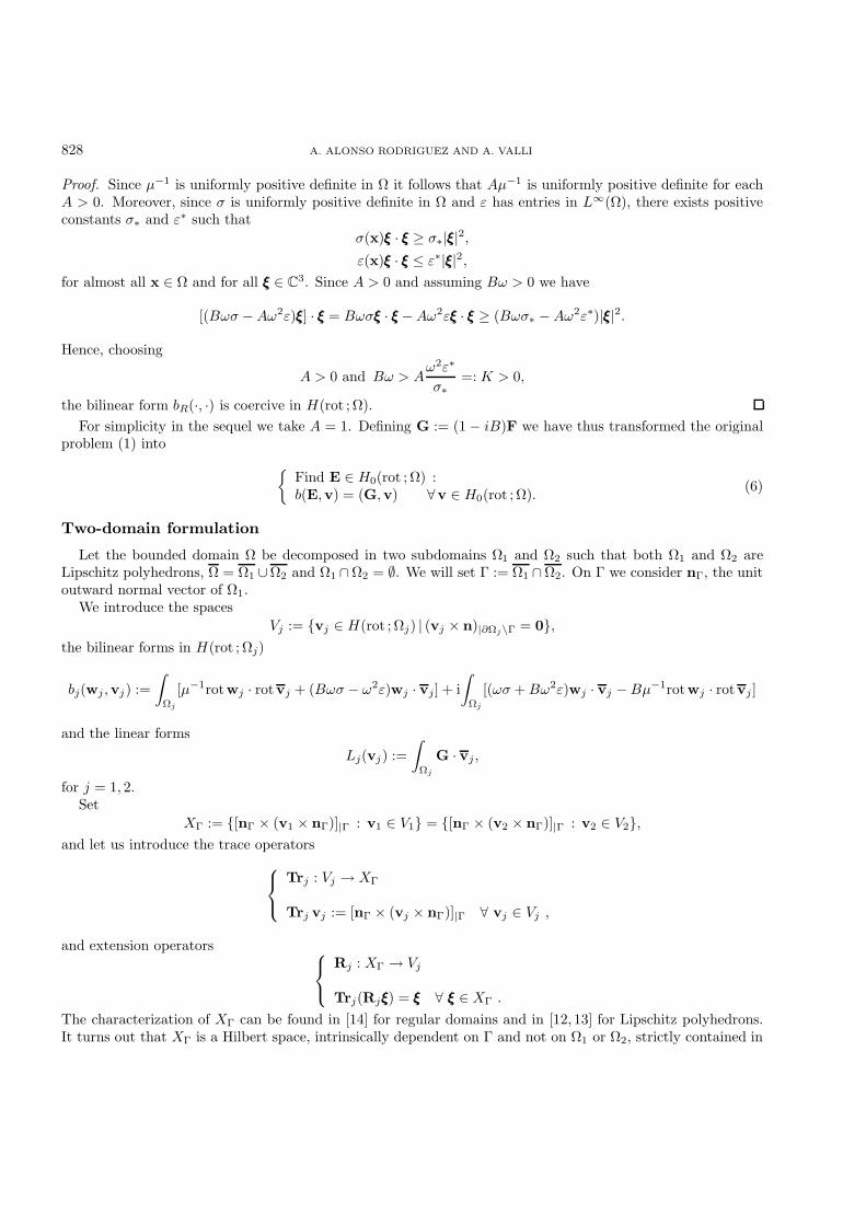
Proof. Since µ−1 is uniformly positive definite in Ω it follows that Aµ−1 is uniformly positive definite for eachA > 0. Moreover, since σ is uniformly positive definite in Ω and ε has entries in L∞(Ω), there exists positiveconstants σ∗ and ε∗ such that

σ(x)ξξξ · ξξξ ≥ σ∗|ξξξ|2,ε(x)ξξξ · ξξξ ≤ ε∗|ξξξ|2,

for almost all x ∈ Ω and for all ξξξ ∈ C3. Since A > 0 and assuming Bω > 0 we have

[(Bωσ −Aω2ε)ξξξ] · ξξξ = Bωσξξξ · ξξξ −Aω2εξξξ · ξξξ ≥ (Bωσ∗ −Aω2ε∗)|ξξξ|2.

Hence, choosing

A > 0 and Bω > Aω2ε∗

σ∗=: K > 0,

the bilinear form bR(·, ·) is coercive in H(rot ; Ω).For simplicity in the sequel we take A = 1. Defining G := (1− iB)F we have thus transformed the original

problem (1) into Find E ∈ H0(rot ; Ω) :b(E,v) = (G,v) ∀v ∈ H0(rot ; Ω). (6)

Two-domain formulation

Let the bounded domain Ω be decomposed in two subdomains Ω1 and Ω2 such that both Ω1 and Ω2 areLipschitz polyhedrons, Ω = Ω1 ∪Ω2 and Ω1 ∩Ω2 = ∅. We will set Γ := Ω1 ∩Ω2. On Γ we consider nΓ, the unitoutward normal vector of Ω1.

We introduce the spacesVj := vj ∈ H(rot ; Ωj) | (vj × n)|∂Ωj\Γ = 0,

the bilinear forms in H(rot ; Ωj)

bj(wj ,vj) :=∫

Ωj

[µ−1rot wj · rot vj + (Bωσ − ω2ε)wj · vj] + i∫

Ωj

[(ωσ +Bω2ε)wj · vj −Bµ−1rot wj · rot vj ]

and the linear forms

Lj(vj) :=∫

Ωj

G · vj ,

for j = 1, 2.Set

XΓ := [nΓ × (v1 × nΓ)]|Γ : v1 ∈ V1 = [nΓ × (v2 × nΓ)]|Γ : v2 ∈ V2,and let us introduce the trace operators Trj : Vj → XΓ

Trj vj := [nΓ × (vj × nΓ)]|Γ ∀ vj ∈ Vj ,

and extension operators Rj : XΓ → Vj

Trj(Rjξξξ) = ξξξ ∀ ξξξ ∈ XΓ .

The characterization of XΓ can be found in [14] for regular domains and in [12, 13] for Lipschitz polyhedrons.It turns out that XΓ is a Hilbert space, intrinsically dependent on Γ and not on Ω1 or Ω2, strictly contained in


(H−1/2(Γ))3, the dual space of (H1/2(Γ))3. Just to give an idea, in the case Γ ∩ ∂Ω = ∅ the characterizationresult reads:

XΓ = ξξξ ∈ (H−1/2(Γ))3 | ξξξ · n = 0 and rot τξξξ ∈ H−1/2(Γ) .

For the construction of continuous extension operators Rj see [2]. There the following assumptions on thegeometry of the domain Ω are required: ∂Ω is Lipschitz and H(rot ; Ω) ∩ H0(div ; Ω) ⊂ (H1(Ω))3. This lasthypothesis is satisfied if ∂Ω ∈ C1,1 or Ω is a convex polyhedron. However, using the results in [12,13] and thesame arguments of [2], it is possible to drop the hypothesis H(rot ; Ω)∩H0(div ; Ω) ⊂ (H1(Ω))3 and to constructa continuous extension operator in a Lipschitz polyhedron, not necessarily convex.

The two-domain formulation of problem (6) reads:

find (E1,E2) ∈ V1 × V2 :

b1(E1,v1) = L1(v1) ∀ v1 ∈ H0(rot ; Ω1)

Tr1 E1 = Tr2 E2

b2(E2,v2) = L2(v2) ∀ v2 ∈ H0(rot ; Ω2)

b2(E2,R2ξξξ) = L2(R2ξξξ) + L1(R1ξξξ)− b1(E1,R1ξξξ) ∀ ξξξ ∈ XΓ .

(7)

The equivalence of the formulations (6) and (7) can be easily proved (see, for instance, Alonso and Valli [3],where a similar situation is considered).

For the numerical approximation we will use the edge elements introduced by Nedelec (see [21] and [22]).They are rot-conforming finite elements. We consider a family of triangulations Thh>0 of Ω matching in theinterface, i.e., we assume that each element of Th only intersects either Ω1 or Ω2. In this way we construct finitedimensional spaces Vj,h ⊂ Vj , V 0

j,h := Vj,h ∩H0(rot ; Ωj) and on the interface we have the finite elements

XΓ,h := [nΓ × (v1,h × nΓ)]|Γ | v1,h ∈ V1,h = [nΓ × (v2,h × nΓ)]|Γ | v2,h ∈ V2,h.

The finite dimensional approximation problem reads:

find (E1,h,E2,h) ∈ V1,h × V2,h :

b1(E1,h,v1,h) = L1(v1,h) ∀ v1,h ∈ V 01,h

Tr1 E1,h = Tr2 E2,h

b2(E2,h,v2,h) = L2(v2,h) ∀ v2,h ∈ V 02,h

b2(E2,h,R2,hξξξh) = L2(R2,hξξξh)+ L1(R1,hξξξh)− b1(E1,h,R1,hξξξh) ∀ ξξξh ∈ XΓ,h ,

(8)

where Rj,h is any extension operator from XΓ,h to Vj,h, j = 1, 2.


3. Non-overlapping domain decomposition methods

Now we consider an abstract problem whose structure is the same of problems (7) and (8):

find (u1, u2) ∈ V1 × V2 :

A1(u1, v1) = L1(v1) ∀ v1 ∈ V01

Tr 1 u1 = Tr 2 u2

A2(u2, v2) = L2(v2) ∀ v2 ∈ V02

A2(u2,R2ξ) = L2(R2ξ) + L1(R1ξ)−A1(u1,R1ξ) ∀ ξ ∈ X ,

(9)

where for j = 1, 2, Vj and X are complex Hilbert spaces, Tr j : Vj → X is a linear and continuous traceoperator, Rj : X → Vj is a linear and continuous extension operator (hence Tr j(Rjξ) = ξ for all ξ ∈ X ),V0j := vj ∈ Vj : Tr jvj = 0 and Lj is a continuous linear form in Vj . Aj is a bilinear form such thatAj(·, ·) = AR,j(·, ·) + iAI,j(·, ·), where AR,j and AI,j are Hermitian and continuous bilinear forms and AR,j iscoercive.

In the sequel we will use the following notation: if X is a complex Hilbert space and X ′ is its dual space, wedenote by (·, ·)X the inner product in X , by ‖ · ‖X the associated norm and by 〈·, ·〉 the duality pairing betweenX ′ and X .

The two-domain problem (9) can be also formulated in term of the Steklov-Poincare operators. For j = 1, 2,we consider the extension Ej : X → Vj defined in the following way: for each ξ ∈ X , Ejξ is the unique solution of

Ejξ ∈ Vj :

Aj(Ejξ, vj) = 0 ∀ vj ∈ V0j

Tr j (Ejξ) = ξ.

Then the local Steklov-Poincare operators Sj : X → X ′ is defined as follows:

〈Sjξ, ν〉 := Aj(Ejξ, Ejν), ∀ ξ, ν ∈ X , (10)

and we also set S = S1 + S2.Let Ψj be the solution of

Ψj ∈ V0j :

Aj(Ψj, vj) = Lj(vj) ∀ vj ∈ V0j .

Now we can define Υ ∈ X ′ as

〈Υ, ξ〉 :=2∑j=1

[Lj(Ejξ)−Aj(Ψj , Ejξ)].

It is clear that the solution of (9) can be written as

uj = Ejζ + Ψj ,

where

(S1 + S2)ζ = Υ. (11)


We are going to construct the solution of (11) as the limit of the Richardson method with a preconditioner.The different algorithms we propose correspond to different preconditioners.

3.1. The γ-Dirichlet/Robin method

This is, in fact, a family of methods depending on a real parameter γ. At each step we have a boundaryvalue problem in Ω1 with a Dirichlet condition on Γ and a boundary value problem in Ω2 with Robin boundarycondition on Γ. Given γ ∈ R, γ ≥ 0, we propose the following iteration: being given ζ0 ∈ X , for each n ≥ 0solve

un+11 ∈ V1 :

A1(un+11 , v1) = L1(v1) ∀ v1 ∈ V0

1

Tr 1 un+11 = ζn,

(12)

then

un+12 ∈ V2 :

A2(un+12 , v2) = L2(v2) ∀ v2 ∈ V0

2

A2(un+12 ,R2ξ) + γ(Tr 2u

n+12 , ξ)X = L2(R2ξ)

+L1(R1ξ)−A1(un+11 ,R1ξ) + γ(Tr 1u

n+11 , ξ)X ∀ ξ ∈ X ,

(13)

finally set

ζn+1 = (1− θ)ζn + θTr 2un+12 . (14)

If, for any k ∈ R we consider the operators Skj : X → X ′

〈Skj ξ, ν〉 := 〈Sjξ, ν〉+ k(ξ, ν)X ,

j = 1, 2, it is easy to see thatSγ2 (Tr 2u

n+12 ) = Υ− S−γ1 ζn,

henceζn+1 = (1− θ)ζn + θ(Sγ2 )−1(Υ− S−γ1 ζn)

= ζn + θ(Sγ2 )−1[Υ− (S−γ1 + Sγ2 )ζn]

= ζn + θ(Sγ2 )−1(Υ− Sζn).

The iterative procedure (12–14) is therefore equivalent to the Richardson method for problem (11) using Sγ2 aspreconditioner. The iteration operator is

Tθ = I − θ(Sγ2 )−1S.

3.2. The γ-Robin/Robin method

We consider another family of methods, depending on a real parameter γ ≥ 0, that will be called γ-Robin/Robin (a generalization of the Neumann/Neumann method [1, 10]): being given ζ0 ∈ X for each n ≥ 0


solve for j = 1, 2 un+1j ∈ Vj :

Aj(un+1j , vj) = Lj(vj) ∀ vj ∈ V0

j

Tr j un+1j = ζn,

(15)

then

Φn+1j ∈ Vj :

Aj(Φn+1j , vj) = 0 ∀ vj ∈ V0

j

Aj(Φn+1j ,Rjξ) + γ(Tr jΦn+1

j , ξ)X = L1(R1ξ)−A1(un+11 ,R1ξ)

+L2(R2ξ)−A2(un+12 ,R2ξ) ∀ ξ ∈ X ,

(16)

finally set

ζn+1 = ζn + θ(Tr 1Φn+11 + Tr 2Φn+1

2 ). (17)

In order to write this iteration as a preconditioned Richardson method for the Steklov-Poincare problem (11),it is easy to see that

Sγj (Tr jΦn+1j ) = Υ− (S1 + S2)ζn, j = 1, 2,

soζn+1 = ζn + θ[(Sγ1 )−1 + (Sγ2 )−1](Υ− Sζn).

Then the iterative procedure (15–17) is equivalent to the Richardson method for problem (11) using [(Sγ1 )−1 +(Sγ2 )−1]−1 as a preconditioner. In particular the iteration operator in (17) is given by

Tθ = I − θ[(Sγ1 )−1 + (Sγ2 )−1]S.

3.3. The modified Neumann/Neumann method

Another domain decomposition method that we can consider is the following modification of Neumann/Neumannmethod: being given ζ0 ∈ X for each n ≥ 0 solve for j = 1, 2

un+1j ∈ Vj :

Aj(un+1j , vj) = Lj(vj) ∀ vj ∈ V0

j

Tr j un+1j = ζn,

(18)

then

Φn+1j ∈ Vj :

AR,j(Φn+1j , vj) = 0 ∀ vj ∈ V0

j

AR,j(Φn+1j ,Rjξ) = L1(R1ξ)−A1(un+1

1 ,R1ξ)+L2(R2ξ)−A2(un+1

2 ,R2ξ) ∀ ξ ∈ X ,

(19)


finally set

ζn+1 = ζn + θ(Tr 1Φn+11 + Tr 2Φn+1

2 ). (20)

We recall that Aj(·, ·) = AR,j(·, ·) + iAI,j(·, ·), where AR,j and AI,j are Hermitian symmetric and continuousbilinear forms and AR,j is coercive.

In order to write the iteration in terms of a preconditioned Richardson method for the Steklov-Poincareproblem (11), we consider a new operator associated to the bilinear forms AR,j(·, ·). For j = 1, 2, let us definethe extension Fj : X → Vj such that for all ξ ∈ X , Fjξ is the unique solution of

Fjξ ∈ Vj :

AR,j(Fjξ, vj) = 0 ∀ vj ∈ V0j

Tr j (Fjξ) = ξ.

Then SR,j : X → X ′ is defined as

〈SR,jξ, ν〉 := AR,j(Fjξ,Fjν) ∀ ξ, ν ∈ X .

It is easy to see thatSR,j(Tr jΦn+1

j ) = Υ− (S1 + S2)ζn,

thereforeζn+1 = ζn + θ(S−1

R,1 + S−1R,2)[Υ− Sζn].

Then the iterative procedure (18–20) is equivalent to the Richardson method for problem (11) using (S−1R,1 +

S−1R,2)−1 as preconditioner. The iterative operator in (20) is given by

Tθ = I − θ(S−1R,1 + S−1

R,2)S.

4. Convergence results

4.1. The γ-Dirichlet/Robin method

In order to prove the convergence of the γ-Dirichlet/Robin method we prove the following abstract result.

Theorem 4.1. Let X be a complex Hilbert space, X ′ its dual space and Q,Q2 : X → X ′ linear operators. Weassume that

1. Q,Q2 are continuous, i.e.,1.a: there exist β > 0 such that

|〈Qη, λ〉| ≤ β‖η‖X‖λ‖X ∀ η, λ ∈ X ,

1.b: there exist β2 > 0 such that

|〈Q2η, λ〉| ≤ β2‖η‖X‖λ‖X ∀ η, λ ∈ X ;

2. Q2 is real coercive, i.e., there exists αR2 > 0 such that

Re〈Q2η, η〉 ≥ αR2‖η‖2X ∀ η ∈ X ;


3. there exists a constant κ∗ > 0 such that

Re[〈Q2η,Q−12 Qη〉+ 〈Qη, η〉] ≥ κ∗‖η‖2X ∀ η ∈ X .

Then for any η0 in X the sequenceηn+1 = ηn − θQ−1

2 Qηn

converges to 0 in X , provided that

0 < θ <κ∗α2

R2

β2β2·

Proof. First we notice that Q2 is coercive because

|〈Q2η, η〉| ≥ |Re〈Q2η, η〉| ≥ αR2‖η‖2X .

Hence from 1.b and 2 there exists Q−12 .

We introduce the scalar product

(η, λ)Q2 :=12

(〈Q2η, λ〉+ 〈Q2λ, η〉),

with the corresponding norm‖η‖2Q2

:= (η, η)Q2 = Re〈Q2η, η〉,which is equivalent to the norm ‖η‖X , i.e.;

αR2‖η‖2X ≤ ‖η‖2Q2≤ β2‖η‖2X .

We shall prove that, choosing θ in a suitable interval, the map Tθ : X → X defined as

Tθη := η − θQ−12 Qη

is a contraction with respect to the norm ‖ · ‖Q2 . Assuming that 0 ≤ θ, we have

‖Tθη‖2Q2= Re[〈Q2η, η〉+ θ2〈Qη,Q−1

2 Qη〉 − θ(〈Q2η,Q−12 Qη〉+ 〈Qη, η〉)]

≤ ‖η‖2Q2+ θ2 β2

αR2‖η‖2X − θκ∗‖η‖2X

≤(

1 + θ2 β2

α2R2

− θκ∗

β2

)‖η‖2Q2

.

By imposing the condition

1 + θ2 β2

α2R2

− θκ∗

β2< 1,

the thesis follows.Now, we are in position to prove

Theorem 4.2. Assuming that for j = 1, 2H1. Aj : Vj × Vj → R is a bilinear form such that

Aj(·, ·) = AR,j(·, ·) + iAI,j(·, ·),


where AR,j and AI,j are Hermitian symmetric and continuous bilinear forms, i.e., there exist constantsΛLj > 0 such that

AL,j(vj , wj) ≤ ΛLj‖vj‖Vj‖wj‖Vj ∀ vj , wj ∈ Vj, L = R, I, j = 1, 2,

and AR,j is coercive, i.e., there exist constants ∆Rj > 0 such that

AR,j(vj , vj) ≥ ∆Rj‖vj‖2Vj ∀ vj ∈ Vj , j = 1, 2 ;

H2. the trace operator Tr j : Vj → X is continuous, i.e., there exist constants CTrj > 0 such that

‖Tr jvj‖X ≤ CTrj‖vj‖Vj ∀ vj ∈ Vj , j = 1, 2 ;

H3. there exist extension operators Rj : X → Vj, which are continuous, i.e., there exist constants CRj > 0such that

‖Rjη‖Vj ≤ CRj‖η‖X ∀ η ∈ X , j = 1, 2,

then there exists γ∗ ∈ R such that for each γ ≥ 0, γ > γ∗ and for each ζ0 ∈ X the iterative scheme (12–14) isconvergent in X , provided that the relaxation parameter θ is chosen in a suitable interval (0, θγ).

Proof. We apply Theorem 4.1 taking

〈Qη, λ〉 = A1(E1η, E1λ) +A2(E2η, E2λ) (Q = S1 + S2)〈Q2η, λ〉 = A2(E2η, E2λ) + γ(η, λ)X (Q2 = Sγ2 ).

In particular,

Re〈Q2η, η〉 = AR,2(E2η, E2η) + γ(η, η)X .

We notice that from H1 and H3 the extension operator used in the definition of the Steklov-Poincare operatoris continuous; in fact,

∆Rj‖Ejη‖2Vj ≤ |Aj(Ejη, Ejη)| = |Aj(Ejη,Rjη)| ≤ (ΛRj + ΛIj)‖Ejη‖Vj‖Rjη‖Vj ,

so

‖Ejη‖Vj ≤ CEj‖η‖X , (21)

with CEj = ΛRj+ΛIj∆Rj

CRj . Hence it is clear that assumptions 1 and 2 of Theorem 4.1 are satisfied with constants

β = (ΛR1 + ΛI1)C2E1 + (ΛR2 + ΛI2)C2

E2

β2 = (ΛR2 + ΛI2)C2E2 + γ =: β2 + γ

αR2 =∆R2

C2Tr2

+ γ =: αR2 + γ.

We notice that β, β2 and αR2 are independent of γ.


Now we shall prove that there exists γ∗ ∈ R such that for each γ > γ∗, and γ ≥ 0 assumption 3 of Theorem 4.1is satisfied. We notice that

Re[〈Q2η,Q−12 Qη〉+ 〈Qη, η〉]

= Re[〈Q2η,Q−12 Qη〉 − 〈Qη, η〉] +Re[〈Qη, η〉+ 〈Qη, η〉]

= 2Re〈Qη, η〉+Re[〈Q2η,Q−12 Qη〉 − 〈Qη, η〉]

≥ 2Re〈Qη, η〉 − |Re[〈Q2η,Q−12 Qη〉 − 〈Qη, η〉]|.

Moreover

Re〈Qη, η〉 = AR1(E1η, E1η) +AR2(E2η, E2η) ≥(∆R1

C2Tr1

+∆R2

C2Tr2

)‖η‖2X = α‖η‖2X ,

where we have set α := ∆R1C2Tr1

+ ∆R2C2Tr2

. Taking λ = Q−12 Qη we have, by a straightforward computation,

|Re[〈Q2η,Q−12 Qη〉 − 〈Qη, η〉]| = |Re[〈Q2η, λ〉 − 〈Q2λ, η〉]|

= |Re[A2(E2η, E2λ) + γ(η, λ)X −A2(E2λ, E2η)− γ(λ, η)X ]|

= |Re[2iAI,2(E2η, E2λ)]| ≤ 2|AI,2(E2η, E2λ)|

≤ 2ΛI2C2E2‖η‖X‖λ‖X = 2βI2‖η‖X‖λ‖X ,

where we have set βI2 := ΛI2C2E2 . Since ‖λ‖X = ‖Q−1

2 Qη‖X ≤ βαR2‖η‖X , we have

Re[〈Q2η,Q−12 Qη〉+ 〈Qη, η〉] ≥ 2

(α− βI2

β

αR2

)‖η‖2X .

We notice that α, β and βI2 do not depend on γ and that αR2 = αR2 + γ with αR2 > 0 independent of γ.Hence, taking γ ≥ 0 and

γ >βI2β

α− αR2 =: γ∗,

assumption 3 of Theorem 4.1 is satisfied with

κ∗(γ) = 2(α− βI2

β

αR2 + γ

)> 0.

Provided that θ ∈ (0, θγ) with

θγ = 2α(αR2 + γ)− βI2β

(β2 + γ)β2(αR2 + γ),

the iterative scheme (12–14) is convergent in X .

4.2. The γ-Robin/Robin method

We state an abstract result that will be used to prove the convergence of the γ-Robin/Robin method.

Theorem 4.3. Let X be a complex Hilbert space, X ′ its dual space and Q,Q1,Q2 : X → X ′ linear operators.We assume that

1. Q and Qj for j = 1, 2, are continuous, i.e.,


1.a: there exist β > 0 such that

|〈Qη, λ〉| ≤ β‖η‖X‖λ‖X ∀ η, λ ∈ X ,

1.b: there exist βj > 0 such that

|〈Qjη, λ〉| ≤ βj‖η‖X‖λ‖X ∀ η, λ ∈ X ;

2. Qj is real coercive for j = 1, 2, i.e., there exist αRj > 0 such that

Re〈Qjη, η〉 ≥ αRj‖η‖2X ∀ η ∈ X .

Assume moreover that the operator N := (Q−11 +Q−1

2 )−1 satisfies the condition

3. there exists a constant κ∗ > 0 such that

Re[〈Nη,N−1Qη〉+ 〈Qη, η〉] ≥ κ∗‖η‖2X ∀ η ∈ X .

Then there exists θ0 > 0 such that for each θ ∈ (0, θ0) and for any given η0 in X the sequence

ηn+1 = ηn − θN−1Qηn

converges to 0 in X .

Proof. As in Theorem 4.1 we notice that, since Qj is real coercive, it is coercive. Hence N is well defined andit is continuous and coercive (see, e.g. [23], p. 108); more precisely,

|〈Nη, λ〉| ≤ βN‖η‖X‖λ‖X ∀ η, λ ∈ X

with βN =(αR1β2

1+ αR2

β22

)−1, and

|〈Nη, η〉| ≥ αN‖η‖2X ∀ η ∈ X

with αN =(αR1β2

1+ αR2

β22

)(1αR1

+ 1αR2

)−2.Now we shall prove that the following bilinear form

(η, λ)N :=12

(〈Nη, λ〉 + 〈Nλ, η〉) ∀ η, λ ∈ X

is a scalar product in X and that the corresponding norm

‖η‖N :=[Re〈Nη, η〉

]1/2is equivalent to the norm ‖η‖X .


Given η ∈ X we set ψ = Nη and for j = 1, 2, λj = Q−1j ψ. Then

‖η‖2N = Re〈Nη, η〉 = Re〈ψ, (Q−11 +Q−1

2 )ψ〉

= Re[〈Q1λ1, λ1〉+ 〈Q2λ2, λ2〉]

≥ αR1‖λ1‖2X + αR2‖λ2‖2X = αR1‖Q−11 ψ‖2X + αR2‖Q−1

2 ψ‖2X

≥(αR1

β21

+αR2

β22

)‖ψ‖2X ′ =

1βN‖Nη‖2X ′

≥ α2NβN‖η‖2X .

Moreover

‖η‖2N = Re〈Nη, η〉 ≤ |〈Nη, η〉| ≤ βN‖η‖2X ,

hence

α2NβN‖η‖2X ≤ ‖η‖2N ≤ βN‖η‖2X .

As in Theorem 4.1, in order to prove the convergence of ηn, we show that the map Tθ : X → X defined as

Tθη := η − θN−1Qη

is a contraction with respect to the norm ‖ · ‖N . Assuming that 0 ≤ θ, we have

‖Tθη‖2N = Re[〈Nη, η〉+ θ2〈Qη,N−1Qη〉 − θ(〈Nη,N−1Qη〉+ 〈Qη, η〉)]

≤ ‖η‖2N + θ2 β2

αN‖η‖2X − θκ∗‖η‖2X

≤(

1 + θ2 β2βNα3N− θ κ

∗

βN

)‖η‖2N .

Setting θ0 = κ∗α3N

β2β2N

we conclude that Tθ is a contraction for all θ ∈ (0, θ0).

Applying Theorem 4.3 we can prove the convergence of the γ-Robin/Robin method.

Theorem 4.4. Assuming that H1, H2 and H3 in Theorem 4.2 hold, there exists γ] ∈ R such that for eachγ ≥ 0, γ > γ] and for each ζ0 ∈ X the iterative scheme (15–17) is convergent in X provided that the relaxationparameter θ is chosen in a suitable interval (0, θ0

γ).

Proof. We apply Theorem 4.3 taking

〈Qη, λ〉 = A1(E1η, E1λ) +A2(E2η, E2λ) (Q = S1 + S2)〈Qjη, λ〉 = Aj(Ejη, Ejλ) + γ(η, λ)X (Qj = Sγj )


for j = 1, 2. As in Theorem 4.2 is easy to see that assumptions 1 and 2 of Theorem 4.3 are satisfied withconstants

β = (ΛR1 + ΛI1)C2E1 + (ΛR2 + ΛI2)C2

E2 ,

βj = (ΛRj + ΛIj)C2Ej + γ =: βj + γ,

αRj =∆Rj

C2Trj

+ γ =: αRj + γ,

j = 1, 2. Note that β, βj and αRj are independent of γ. Hence we shall show that there exists γ] ∈ R such thatfor γ > γ] and γ ≤ 0, assumption 3 of Theorem 4.3 is satisfied.

Setting λj = Q−1j Nη, νj = Q−1

j Qη we have

|Re[〈Nη,N−1Qη〉 − 〈Qη, η〉]|

= |Re[〈Q1λ1, ν1〉+ 〈Q2λ2, ν2〉 − 〈Q1ν1, λ1〉 − 〈Q2ν2, λ2〉]|

= |Re[2iAI,1(E1λ1, E1ν1) + 2iAI,2(E2λ2, E2ν2)]|

≤ 2|AI,1(E1λ1, E1ν1) +AI,2(E2λ2, E2ν2)|

≤ 2(ΛI1C2E1‖Q

−11 Nη‖X‖Q−1

1 Qη‖X + ΛI2C2E2‖Q

−12 Nη‖X‖Q−1

2 Qη‖X )

≤ 2(ΛI1C2

E1α2R1

+ΛI2C2

E2α2R2

)‖Nη‖X‖Qη‖X

≤ 2(ΛI1C2

E1α2R1

+ΛI2C2

E2α2R2

)βNβ‖η‖2X .

Hence, setting βIj := ΛIjC2Ej

|Re[〈Nη,N−1Qη〉+ 〈Qη, η〉]| ≥ 2[α−

( βI1α2R1

+βI2α2R2

)βNβ

]‖η‖2X = 2κ∗(γ)‖η‖2X ,

whereκ∗(γ) = 2

[α−

( βI1(αR1 + γ)2

+βI2

(αR2 + γ)2

)( αR1 + γ

(β1 + γ)2+

αR2 + γ

(β2 + γ)2

)−1

β],

with α, β, βIj , βj and αRj independent on γ. Since( βI1(αR1 + γ)2

+βI2

(αR2 + γ)2

)( αR1 + γ

(β1 + γ)2+

αR2 + γ

(β2 + γ)2

)−1

tends to zero when γ tends to infinity, there exist γ] such that κ∗(γ) > 0 for each γ > γ].

4.3. The modified Neumann/Neumann method

We can also prove the following:

Theorem 4.5. Let X be a complex Hilbert space, X ′ its dual space and Q, P1, P2 : X → X ′ linear operators.Suppose that for j = 1, 2, Pj is Hermitian symmetric, i.e., 〈Pjη, λ〉 = 〈Pjλ, η〉 for each η, λ ∈ X . We assumethat


1. Q is continuous, i.e., there exist β > 0 such that

|〈Qη, λ〉| ≤ β‖η‖X‖λ‖X ∀ η, λ ∈ X ;

2. for j = 1, 2, Pj is continuous and coercive, i.e.,2.a: there exist βPj > 0 such that

|〈Pjη, λ〉| ≤ βPj‖η‖X‖λ‖X ∀ η, λ ∈ X ,

2.b: there exist αPj > 0 such that

〈Pjη, η〉 ≥ αPj‖η‖2X ∀ η ∈ X ;

3. Q is real coercive, i.e. there exist αR > 0 such that

Re〈Qη, η〉 ≥ αR‖η‖2X ∀ η ∈ X .

Then there exists θ0 such that for each θ ∈ (0, θ0) and for any η0 in X the sequence

ηn+1 = ηn − θ(P−11 + P−1

2 )−1Qηn

converges to 0 in X .

The proof is similar to that of Theorem 4.3, taking Pj instead of Qj, and taking into account that theoperators Pj are Hermitian symmetric.

Assuming that H1, H2 and H3 of Theorem 4.2 are satisfied, the convergence of the iterative scheme (18–20)can be proven by applying Theorem 4.5 with

Q = S1 + S2

Pj = SR,j , j = 1, 2.

5. Application to time-harmonic Maxwell equations and other problems

Going back to the discrete time-harmonic Maxwell problem, the γ-Dirichlet/Robin procedure reads: beinggiven ζζζ0

h ∈ XΓ,h, for n ≥ 0 solveEn+1

1,h ∈ V1,h :

b1(En+11,h ,v1,h) = L1(v1,h) ∀ v1,h ∈ V 0

1,h

Tr1 En+11,h = ζζζnh,

(22)

then

En+12,h ∈ V2,h :

b2(En+12,h ,v2,h) = L2(v2,h) ∀ v2,h ∈ V 0

2,h

b2(En+12,h ,R2,hξξξh) + γ(Tr2 En+1

2,h , ξξξh)XΓ = L2(R2,hξξξh)+L1(R1,hξξξh)− b1(En+1

1,h ,R1,hξξξh) + γ(Tr1 En+11,h , ξξξh)XΓ ∀ ξξξh ∈ XΓ,h ,

(23)


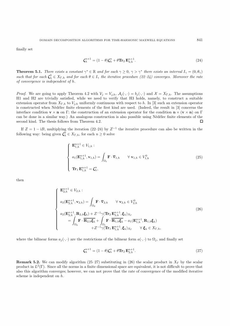
finally set

ζζζn+1h = (1− θ)ζζζnh + θTr2 En+1

2,h . (24)

Theorem 5.1. There exists a constant γ∗ ∈ R and for each γ ≥ 0, γ > γ∗ there exists an interval Iγ = (0, θγ)such that for each ζζζ0

h ∈ XΓ,h and for each θ ∈ Iγ the iterative procedure (22–24) converges. Moreover the rateof convergence is independent of h.

Proof. We are going to apply Theorem 4.2 with Vj = Vj,h, Aj(·, ·) = bj(·, ·) and X = XΓ,h. The assumptionsH1 and H2 are trivially satisfied, while we need to verify that H3 holds, namely, to construct a suitableextension operator from XΓ,h to Vj,h uniformly continuous with respect to h. In [3] such an extension operatoris constructed when Nedelec finite elements of the first kind are used. (Indeed, the result in [3] concerns theinterface condition v × n on Γ; the construction of an extension operator for the condition n × (v × n) on Γcan be done in a similar way.) An analogous construction is also possible using Nedelec finite elements of thesecond kind. The thesis follows from Theorem 4.2.

If Z = 1 − iB, multiplying the iteration (22–24) by Z−1 the iterative procedure can also be written in thefollowing way: being given ζζζ0

h ∈ XΓ,h, for each n ≥ 0 solve

En+11,h ∈ V1,h :

a1(En+11,h ,v1,h) =

∫Ω1

F · v1,h ∀ v1,h ∈ V 01,h

Tr1 En+11,h = ζζζnh ,

(25)

then

En+12,h ∈ V2,h :

a2(En+12,h ,v2,h) =

∫Ω2

F · v2,h ∀ v2,h ∈ V 02,h

a2(En+12,h ,R2,hξξξh) + Z−1γ(Tr2 En+1

2,h , ξξξh)XΓ

=∫

Ω2

F ·R2,hξξξh +∫

Ω1

F ·R1,hξξξh − a1(En+11,h ,R1,hξξξh)

+Z−1γ(Tr1 En+11,h , ξξξh)XΓ ∀ ξξξh ∈ XΓ,h,

(26)

where the bilinear forms aj(·, ·) are the restrictions of the bilinear form a(·, ·) to Ωj, and finally set

ζζζn+1h = (1− θ)ζζζnh + θTr2 En+1

2,h . (27)

Remark 5.2. We can modify algorithm (25–27) substituting in (26) the scalar product in XΓ by the scalarproduct in L2(Γ). Since all the norms in a finite dimensional space are equivalent, it is not difficult to prove thatalso this algorithm converges; however, we can not prove that the rate of convergence of the modified iterativescheme is independent on h.


The γ-Robin/Robin method for the discrete time-harmonic Maxwell problem reads: being given ζζζ0h ∈ XΓ,h,

for n ≥ 0 solve for j = 1, 2 En+1j,h ∈ Vj,h :

bj(En+1j,h ,vj,h) = Lj(vj,h) ∀ vj,h ∈ V 0

j,h

Trj En+1j,h = ζζζnh,

(28)

then

ΦΦΦn+1j,h ∈ Vj,h :

bj(ΦΦΦn+1j,h ,vj,h) = 0 ∀ vj,h ∈ V 0

j,h

bj(ΦΦΦn+1j,h ,Rj,hξξξh) + γ(TrjΦΦΦ

n+1j,h , ξξξh)XΓ = L1(R1,hξξξh)

−b1(En+11,h ,R1,hξξξh) + L2(R2,hξξξh)− b2(En+1

2,h ,R2,hξξξh) ∀ ξξξh ∈ XΓ,h ,

(29)

and finally set

ζζζn+1h = ζζζnh + θ(Tr1 ΦΦΦn+1

1,h + Tr2 ΦΦΦn+12,h ). (30)

Theorem 5.3. There exist a constant γ] ∈ R and for each γ ≥ 0, γ > γ] there exist an interval Iγ = (0, θ0γ)

such that for each ζζζ0h ∈ XΓ,h and for each θ ∈ Iγ the iterative procedure (28–30) converges. Moreover the rate

of convergence is independent of h.

Proof. The result is based on Theorem 4.4. In the proof of Theorem 5.1, we have already verified that H1-H3are satisfied.

As for the γ-Dirichlet/Robin method, by multiplying (28) and (29) by Z−1 we can write the γ-Robin/Robinmethod using the original bilinear form a(·, ·). Moreover, we can substitute in (29) the scalar product in XΓ,h

by the scalar product in L2(Γ), at the cost of loosing the proof that the rate convergence is independent of h.

The modified Neumann/Neumann method for the discrete time-harmonic Maxwell problem reads: beinggiven ζζζ0

h ∈ XΓ,h, for n ≥ 0 solve for j = 1, 2En+1j,h ∈ Vj,h :

bj(En+1j,h ,vj,h) = Lj(vj,h) ∀ vj,h ∈ V 0

j,h

Trj En+1j,h = ζζζnh,

(31)

then

ΦΦΦn+1j,h ∈ Vj,h :

bR,j(ΦΦΦn+1j,h ,vj,h) = 0 ∀ vj,h ∈ V 0

j,h

bR,j(ΦΦΦn+1j,h ,Rj,hξξξh) = L1(R1,hξξξh)− b1(En+1

1,h ,R1,hξξξh)+L2(R2,hξξξh)− b2(En+1

2,h ,R2,hξξξh) ∀ ξξξh ∈ XΓ,h ,

(32)


and finally set

ζζζn+1h = ζζζnh + θ(Tr1 ΦΦΦn+1

1,h + Tr2 ΦΦΦn+12,h ). (33)

By means of Theorem 4.5, the following result can be proved.

Theorem 5.4. There exist θ0 > 0 such that for each θ ∈ (0, θ0) the iterative procedure (31–33) converges.Moreover the rate of convergence is independent of h.

Finally, we notice that these three domain decomposition methods can be applied to other boundary valueproblems: for instance, the wave problem in the frequency domain, and the time-harmonic Maxwell equationsin a conductor with Robin boundary conditions.

The wave problem in the frequency domain

The problem reads (see [17]): −∆u− P u+ iQu = f on Ω

∂u

∂n−M1 u+ iM2 u = 0 in ∂Ω,

with P , Q ∈ L∞(Ω), M1, M2 ∈ L∞(∂Ω), and

Q(x) ≥ Q0 > 0 for almost all x ∈ Ω

M2(x′) ≥M2,0 > 0 for almost all x′ ∈ ∂Ω.

Assuming that f ∈ L2(Ω), the weak formulation of this problem reads find u ∈ H1(Ω) :

c(u, v) = g(v) ∀ v ∈ H1(Ω),(34)

where

c(w, v) :=∫

Ω

(∇w · ∇v − P w v)−∫∂Ω

M1w v + i[∫

Ω

Qwv +∫∂Ω

M2w v

]and

g(v) :=∫

Ω

f v.

The bilinear form c(·, ·) is complex valued, continuous and coercive, but it is not Hermitian symmetric andreal coercive. However, by multiplying it by an appropriate complex constant we can arrive to an equivalentformulation of problem (34) for which the arguments of Sections 3 and 4 can be repeated.

For the numerical approximation of problem (34) the standard Lagrange finite elements can be used. Itis well-known that for this kind of finite elements defined on a regular family of triangulations Thh>0 of Ωwhich induces a quasi-uniform family of triangulations on Γ, assumption H3 of Theorem 4.2 is satisfied witha constant independent of h (see, for instance, [8, 11, 19]). Moreover it is clear that assumptions H1 and H2are satisfied with constants independent of h; hence, also for problem (34) we can prove the results reported inTheorems 5.1, 5.3 and 5.4.

The time-harmonic Maxwell equations with damping with Robin boundary conditions

This problems reads (see [15,16] for the case σ = 0) rot (µ−1rot U)− ω2εU + iωσU = iωJ on Ω

µ−1rot U× n + iω n× (U× n) = g in ∂Ω,


where J ∈ (L2(Ω))3, g ∈ (L2(∂Ω))3 and (g · n)|∂Ω = 0.We consider the space

H(Ω) := v ∈ H(rot ; Ω) | (v × n)|∂Ω ∈ (L2(∂Ω))3,with the norm

‖v‖H(Ω) :=(‖v‖2L2(Ω) + ‖rotv‖2L2(Ω) + ‖v× n‖2L2(∂Ω)

)1/2.

The weak formulation of this problem reads find U ∈ H(Ω) :

d(U,v) = G(v) ∀v ∈ H(Ω),(35)

where

d(w,v) := a(w,v) + iω∫∂Ω

(w × n) · (v × n),

a(·, ·) is defined in (4), and

G(v) := iω∫

Ω

J · v +∫∂Ω

(g× n) · (v× n).

The bilinear form d(·, ·) is complex valued, continuous and coercive, but it is not Hermitian symmetric and realcoercive. Then we need to multiply it by an appropriate complex constant in order to repeat the arguments ofSections 3 and 4.

With the technical assumption Γ∩ ∂Ω = ∅ it is easy to see that, using the same finite elements employed forproblem (8), Theorems 5.1, 5.3 and 5.4 still hold for problem (35).

6. Numerical tests

In this Section we present some numerical tests illustrating the performances of the algorithms we haveproposed. We consider very simple geometric situations, with the only aim of verifying that the convergence ofthe domain decomposition schemes is achieved, uniformly with respect to the mesh size h.

In particular, we have considered the simplest algorithms, always choosing the parameter γ equal to 0:though this situation is not covered by the theory presented here, this choice is the easiest to implement andreduces the γ-Dirichlet/Robin and the γ-Robin/Robin iterative schemes to the well-known Dirichlet/Neumannand Neumann/Neumann ones, respectively. Numerical evidence will show that both the Dirichlet/Neumannand the Neumann/Neumann schemes are indeed convergent, with a rate independent of the mesh size, andthe number of iterations is in general extremely small (provided that the acceleration parameter θ is properlychosen). Consequently, it is apparent that other choices of the parameter γ are not necessary in numericalcomputations.

The computational domain is always the parallelepiped Ω = (0, 2)× (0, 1)× (0, 1), which will be decomposedinto two subdomains Ω1 = (0, xΓ) × (0, 1) × (0, 1) and Ω2 = (xΓ, 2)) × (0, 1) × (0, 1). The numerical meshis uniform, and each element of the grid is a cube of side h. We employ the edge elements of Nedelec type(see [21]), with 12 degrees of freedom for each element, one for each edge.

We consider three types of model problems: the first and most important one is the boundary value problem rot rot u + ω(iσ − ω) u = f in Ω

u× n = g on ∂Ω ,(36)

which is the complete problem (2), (3) (taking, for simplicity, µ = 1, ε = 1).


The second model problem is rot rot u + i u = f in Ω

u× n = g on ∂Ω ,(37)

which is the low-frequency problem analysed in [3] (here we have taken, for simplicity, µ = 1, σ = 1 and ω = 1).In [3] we have proved that in this case the convergence of the Dirichlet/Neumann scheme is achieved, uniformlywith respect to the mesh size h.

The third model problem is rot rot u + u = f in Ω

u× n = g on ∂Ω .(38)

This is the best possible test case for the Dirichlet/Neumann iterative scheme for rot -conforming finite elements,as the weak form associated to the operator rot rot + I is the scalar product in H(rot ; Ω), and therefore theproblem is hermitian and coercive. In this case, the theoretical results assure that the Dirichlet/Neumannscheme is convergent, uniformly in h (see [23], Chap. 4).

For the numerical computations we used the standard tool-box sparfun of MATLABTM 5.2. In particular,for solving the linear systems we adopt the gmres function, with TOL = 10−6.

In the iteration-by-subdomain procedure, we have used the following stopping test

2∑i=1

||uk+1i,h − uki,h||2H(rot ;Ωi)

||uk+1i,h ||2H(rot ;Ωi)

≤ 10−4 . (39)

The first numerical test concerns the exact solution u(x, y, z) = (z2, x2, y2) (having computed consequently thedata f and g). We have considered problems (36), (37) and (38) (the first one with σ = 1 and ω = 1), withdifferent values of h (corresponding to the degrees of freedom indicated in Table 6.1).

Table 6.1. Choice of the mesh size h(the correspondent degrees of freedom are also indicated).

h 1/4 1/6 1/8 1/10 1/12 1/14

DOF 240 960 2464 5040 8976 14560

Choosing xΓ = 0.5, θ = 0.5, the number of iterations of the 0-DR (DN) method has been always equal to 4.We have repeated the computations for two other exact solutions (u(x, y, z) = (sin z, cosx, ey), u(x, y, z) =

(ez sin(xy), (y + z)ex, cos(xz))), for all problems (36), (37) and (38) (the first one with σ = 1 and ω = 1), andh as in Table 6.1. For the set of problems with the exact solution u(x, y, z) = (sin z, cosx, ey) we have takenxΓ = 0.5, and for the set of problems with the exact solution u(x, y, z) = (ez sin(xy), (y+ z)ex, cos(xz)) we havetaken xΓ = 1.5. Choosing as before θ = 0.5, the convergence results have been quite similar (always 4 iterationsto achieve convergence).

It is worthy of noting that the best choice of the relaxation parameter θ seems to be always very close to 0.5.The next computations are made for the exact solution u(x, y, z) = (z2, x2, y2) of problem (36) (again withσ = 1 and ω = 1), having chosen xΓ = 4/3.


Table 6.2. Number of iterations for the 0-DR (DN) methodfor different values of θ and h.

θ \ h (DOF ) 1/3 (84) 1/6 (960) 1/9 (3600)

0.4 5 6 60.45 5 5 50.5 4 4 4

0.55 4 5 50.6 5 6 6

For the solution u(x, y, z) = (sin z, cosx, ey), taking h = 1/6 (DOF = 960), the best choice of θ is reportedin Tables 6.3 and 6.4. Note that only choosing θ very close to 0.5 in problem (38) we have been able to obtaina better rate of convergence than in the case θ = 0.5.

Table 6.3. Number of iterations for the 0-DR (DN) methodfor different values of θ and xΓ (problem (36)).

θ \ xΓ 4/3 2/3

0.3 8 70.4 6 50.5 4 40.6 6 60.7 8 9

Table 6.4. Number of iterations for the 0-DR (DN) methodfor different values of θ and xΓ (problem (38)).

θ \ xΓ 4/3 2/3

0.3 7 70.4 5 5

0.495 4 30.5 4 4

0.504 3 40.6 6 60.7 8 8

These results lead to a significant conclusion: in all cases we have analysed, the choice of relaxation parameterθ equal to 0.5 can be considered optimal for the Dirichlet/Neumann method. Moreover, the method is quiteefficient also for a wide range of values of θ.

We have also verified that the 0-Robin/Robin scheme (which indeed is coincident with the classicalNeumann/Neumann scheme) is extremely efficient. In fact, we have considered the same exact solutions thanbefore for problem (36) (with σ = 1 and ω = 1), choosing xΓ = 1.5, θ = 0.25 (which seems to be optimal forthe Neumann/Neumann method), and the values of h indicated in Table 6.1. In all these cases, the number ofiterations has been always equal to 3.

The results for the modified Neumann/Neumann iterative scheme are less interesting. We have consideredthe exact solutions u(x, y, z) = (sin z, cosx, ey) and u(x, y, z) = (ez sin(xy), (y + z)ex, cos(xz)) for problem (36)(with σ = 1 and ω = 1). Choosing xΓ = 1, the convergence results are reported in Tables 6.5 and 6.6.


Table 6.5. Number of iterations for the modified Neumann/Neumann methodfor different values of θ and h (u(x, y, z) = (sin z, cosx, ey)).

θ \ h 1/4 1/6 1/8

0.05 33 35 370.10 NO NO NO0.25 NO NO NO

Table 6.6. Number of iterations for the modified Neumann/Neumann methodfor different values of θ and h (u(x, y, z) = (ez sin(xy), (y + z)ex, cos(xz))).

θ \ h 1/4 1/6 1/8

0.05 279 276 2760.10 NO NO NO0.25 NO NO NO

One can see that, as predicted by the theory, the scheme is indeed convergent for a suitable (interval of) θ.However, since this value is rather small, convergence is quite slow. The reason is that the preconditioneris relatively different from the given operator (the latter is not hermitian nor real coercive, the former isreal, symmetric and coercive). As a consequence, its preconditioning properties are poor (though the rate ofconvergence is in fact independent of h).

In conclusion, the computations performed show that both the Dirichlet/Neumann and Neumann/Neumanniterative schemes, though not covered by the theory, are extremely efficient and robust domain decompositionmethods for the time-harmonic Maxwell equations with damping.

References

[1] V.I. Agoshkov and V.I. Lebedev, Poincare-Steklov operators and the methods of partition of the domain in variational problems,in Vychisl. Protsessy Sist. (Computational processes and systems), G.I. Marchuk, Ed., Nauka, Moscow 2 (1985) 173–227 (inRussian).

[2] A. Alonso and A. Valli, Some remarks on the characterization of the space of tangential traces of H(rot ; Ω) and the constructionof an extension operator. Manuscripta Math. 89 (1996) 159–178.

[3] A. Alonso and A. Valli, An optimal domain decomposition preconditioner for low-frequency time-harmonic Maxwell equations.Math. Comp. 68 (1999) 607–631.

[4] A. Alonso and A. Valli, A domain decomposition approach for heterogeneous time-harmonic Maxwell equations. Comput.Methods Appl. Mech. Engrg. 143 (1997) 97–112.

[5] A. Alonso, R.L. Trotta and A. Valli, Coercive domain decomposition algorithms for advection–diffusion equations and systems.J. Comput. Appl. Math. 96 (1998) 51–76.

[6] L.C. Berselli, Some topics in fluid mechanics. Ph.D. thesis, Dipartimento di Matematica, Universita di Pisa, Italy (1999).[7] L.C. Berselli and F. Saleri, New substructuring domain decomposition methods for advection–diffusion equations. J. Comput.

Appl. Math. 116 (2000) 201–220.[8] P.E. Bjørstad and O.B. Widlund, Iterative methods for the solution of elliptic problems on regions partitioned into substruc-

tures. SIAM J. Numer. Anal. 23 (1986) 1097–1120.[9] A. Bossavit, Electromagnetisme, en vue de la modelisation. Springer–Verlag, Paris (1993).

[10] J.-F. Bourgat, R. Glowinski, P. Le Tallec and M. Vidrascu, Variational formulation and algorithm for trace operator in domaindecomposition calculations, in Domain Decomposition Methods, T.F. Chan et al., Eds., SIAM, Philadelphia (1989) 3–16.

[11] J.H. Bramble, J.E. Pasciak and A.H. Schatz, An iterative method for elliptic problems on regions partitioned into substructures.Math. Comp. 46 (1986) 361–369.

[12] A. Buffa and P. Ciarlet, Jr., On traces for functional spaces related to Maxwell’s equations Part I: An integration by partsformula in Lipschitz polyhedra. Math. Methods Appl. Sci. 24 (2001) 9–30.

[13] A. Buffa and P. Ciarlet, Jr., On traces for functional spaces related to Maxwell’s equations Part II: Hodge decompositions onthe boundary of Lipschitz polyhedra and applications. Math. Meth. Appl. Sci. 24 (2001) 31–48.


[14] M. Cessenat, Mathematical methods in electromagnetism: Linear theory and applications. World Scientific Pub. Co., Singapore(1996).

[15] P. Collino, G. Delbue, P. Joly and A. Piacentini, A new interface condition in the non-overlapping domain decompositionmethod for the Maxwell equation. Comput. Methods Appl. Mech. Engrg. 148 (1997) 195–207.

[16] B. Despres, P. Joly and J.E. Roberts, A domain decomposition method for the harmonic Maxwell equation, in IterativeMethods in Linear Algebra, R. Beaurvens and P. de Groen, Eds., North Holland, Amsterdam (1992) 475–484.

[17] S. Kim, Domain decomposition iterative procedures for solving scalar waves in the frequency domain. Numer. Math. 79 (1998)231–259.

[18] R. Leis, Exterior boundary-value problems in mathematical physics, in Trends in Applications of Pure Mathematics to Me-chanics 11, H. Zorski, Ed., Pitman, London (1979) 187–203.

[19] L.D. Marini and A. Quarteroni, A relaxation procedure for domain decomposition methods using finite elements. Numer.Math. 55 (1989) 575–598.

[20] P. Monk, A finite element method for approximating the time-harmonic Maxwell equations. Numer. Math. 63 (1992) 243–261.[21] J.C. Nedelec, Mixed finite elements in R3. Numer. Math. 35 (1980) 315–341.[22] J.C. Nedelec, A new family of mixed finite elements in R3. Numer. Math. 50 (1986) 57–81.[23] A. Quarteroni and A. Valli, Domain decomposition methods for partial differential equations. Oxford University Press, Oxford

(1999).[24] J.E. Santos, Global and domain-decomposed mixed methods for the solution of Maxwell’s equations with application to

magnetotellurics. Numer. Methods. Partial Differ. Equations 14 (1998) 407–437.[25] A. Toselli, Domain decomposition methods for vector field problems. Ph.D. thesis, Courant Institute, New York University,

New York (1999).

To access this journal online:www.edpsciences.org

domain decomposition algorithms for time …...domain decomposition algorithms for time-harmonic...

Documents