Last Updated November 2015

DOING MORE WITH EXCEL: MICROSOFT OFFICE 2013 GETTING STARTED PAGE 02 Prerequisites What You Will Learn MORE TASKS IN MICROSOFT EXCEL PAGE 03 Cutting, Copying, and Pasting Data Basic Formulas Filling Data Across Columns and Rows MORE ABOUT FORMATTING CELLS PAGE 08 Numbers Alignment Borders Colors and Patterns MORE PRACTICE WITH FORMULAS AND FUNCTIONS PAGE 13 Functions Create Charts and Graphs Multiple Sheets CLOSING MICROSOFT EXCEL PAGE 18 Saving Spreadsheets Printing Spreadsheets Finding More Help Closing the Program

To complete feedback forms, and to view our full schedule, handouts, and additional tutorials, visit our website:

cws.web.unc.edu

2

GETTING STARTED Prerequisites It is assumed that the user is both familiar and comfortable with the following prior to this class:

• Using the mouse and left-click feature • Basic navigation through Microsoft Windows • Basic typing and keyboard commands • Basic components of Microsoft Excel

Please let the instructor know if you do not meet these requirements. You may still attend the class, but the instructor may not have time to cover all of the prerequisites. What You Will Learn

Cutting, Copying, and Pasting Data

Filling Data Across Columns and Rows

More About Formatting Cells

Formatting Numbers Text Alignment Borders

Colors and Patterns More Practice with Formulas and Functions Functions

Create Charts and Graphs Multiple Sheets Saving Spreadsheets

Formulas Finding More Help Closing the Program

3

MORE TASKS IN MICROSOFT EXCEL Cutting, Copying, and Pasting Data

In the Excel Basics class, we discussed entering data by typing in the cells of an Excel spreadsheet. You can do this either by clicking on a cell and beginning to type, or by typing in the Formula Bar at the top of the screen below the ribbon menu.

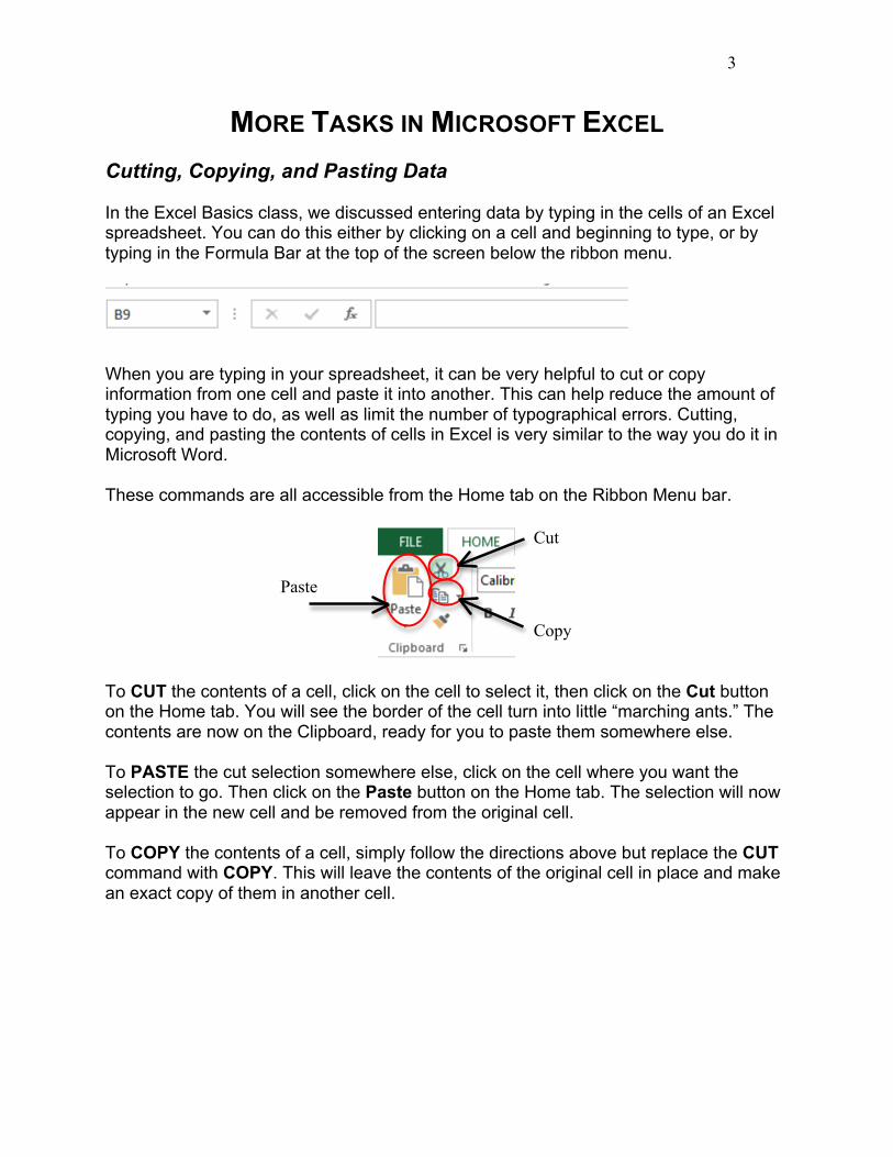
When you are typing in your spreadsheet, it can be very helpful to cut or copy information from one cell and paste it into another. This can help reduce the amount of typing you have to do, as well as limit the number of typographical errors. Cutting, copying, and pasting the contents of cells in Excel is very similar to the way you do it in Microsoft Word. These commands are all accessible from the Home tab on the Ribbon Menu bar.

To CUT the contents of a cell, click on the cell to select it, then click on the Cut button on the Home tab. You will see the border of the cell turn into little “marching ants.” The contents are now on the Clipboard, ready for you to paste them somewhere else. To PASTE the cut selection somewhere else, click on the cell where you want the selection to go. Then click on the Paste button on the Home tab. The selection will now appear in the new cell and be removed from the original cell. To COPY the contents of a cell, simply follow the directions above but replace the CUT command with COPY. This will leave the contents of the original cell in place and make an exact copy of them in another cell.

Paste

Cut

Copy

4

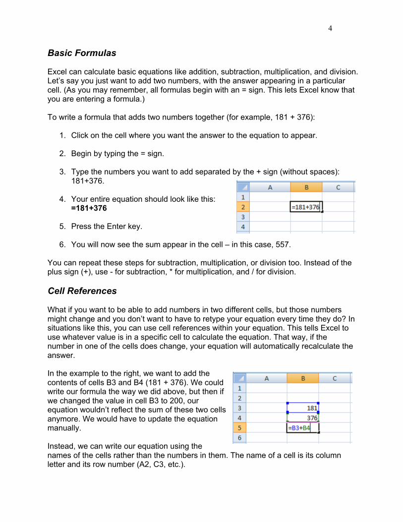
Basic Formulas Excel can calculate basic equations like addition, subtraction, multiplication, and division. Let’s say you just want to add two numbers, with the answer appearing in a particular cell. (As you may remember, all formulas begin with an = sign. This lets Excel know that you are entering a formula.) To write a formula that adds two numbers together (for example, 181 + 376):

1. Click on the cell where you want the answer to the equation to appear.

2. Begin by typing the = sign.

3. Type the numbers you want to add separated by the + sign (without spaces): 181+376.

4. Your entire equation should look like this: =181+376

5. Press the Enter key.

6. You will now see the sum appear in the cell – in this case, 557. You can repeat these steps for subtraction, multiplication, or division too. Instead of the plus sign (+), use - for subtraction, * for multiplication, and / for division. Cell References What if you want to be able to add numbers in two different cells, but those numbers might change and you don’t want to have to retype your equation every time they do? In situations like this, you can use cell references within your equation. This tells Excel to use whatever value is in a specific cell to calculate the equation. That way, if the number in one of the cells does change, your equation will automatically recalculate the answer. In the example to the right, we want to add the contents of cells B3 and B4 (181 + 376). We could write our formula the way we did above, but then if we changed the value in cell B3 to 200, our equation wouldn’t reflect the sum of these two cells anymore. We would have to update the equation manually. Instead, we can write our equation using the names of the cells rather than the numbers in them. The name of a cell is its column letter and its row number (A2, C3, etc.).

5

To write a formula using cell references:

1. Type the numbers you want to add in two different cells.

2. Click on the cell where you want the answer to the equation to appear.

3. Begin the equation by typing the = sign.

4. Either click on or type in the name of the cell with the first number to be added (in this example, B3).

5. Type the + sign.

6. Either click on or type in the name of the cell with the second number to be added (in this example, B4). Your equation should look like this: =B3+B4

7. Press the Enter key.

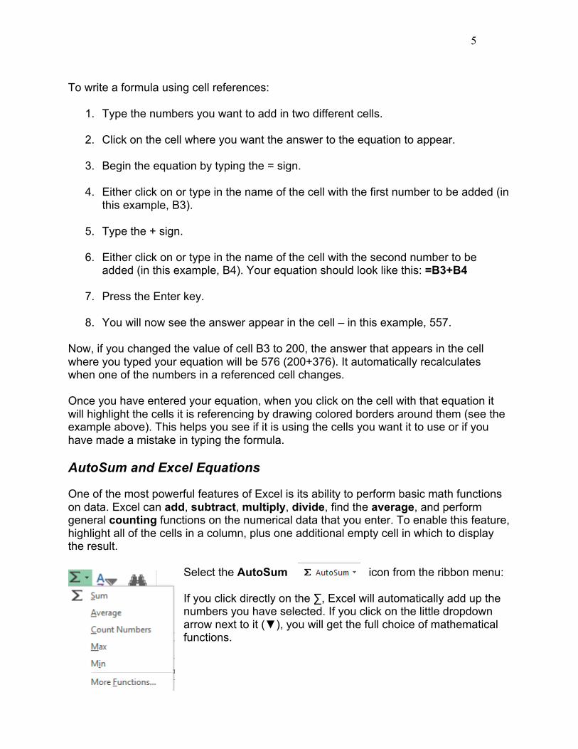
8. You will now see the answer appear in the cell – in this example, 557. Now, if you changed the value of cell B3 to 200, the answer that appears in the cell where you typed your equation will be 576 (200+376). It automatically recalculates when one of the numbers in a referenced cell changes. Once you have entered your equation, when you click on the cell with that equation it will highlight the cells it is referencing by drawing colored borders around them (see the example above). This helps you see if it is using the cells you want it to use or if you have made a mistake in typing the formula. AutoSum and Excel Equations One of the most powerful features of Excel is its ability to perform basic math functions on data. Excel can add, subtract, multiply, divide, find the average, and perform general counting functions on the numerical data that you enter. To enable this feature, highlight all of the cells in a column, plus one additional empty cell in which to display the result.

Select the AutoSum icon from the ribbon menu: If you click directly on the ∑, Excel will automatically add up the numbers you have selected. If you click on the little dropdown arrow next to it (▼), you will get the full choice of mathematical functions.

6

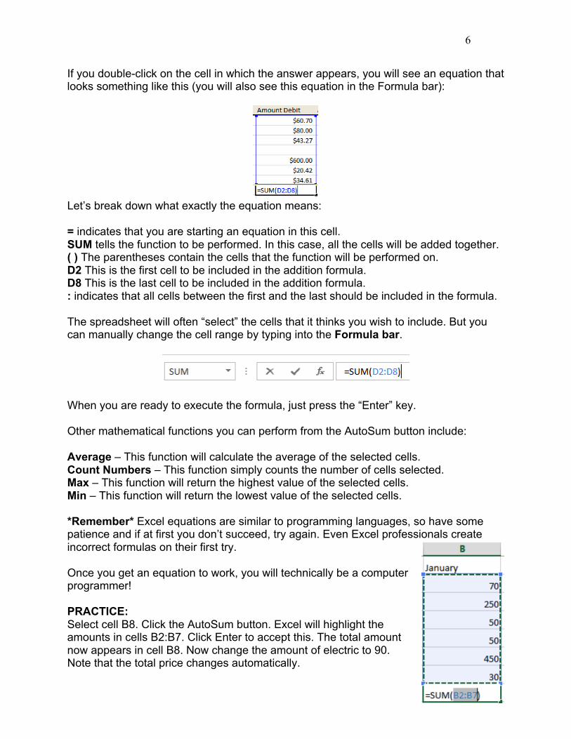
If you double-click on the cell in which the answer appears, you will see an equation that looks something like this (you will also see this equation in the Formula bar):

Let’s break down what exactly the equation means: = indicates that you are starting an equation in this cell. SUM tells the function to be performed. In this case, all the cells will be added together. ( ) The parentheses contain the cells that the function will be performed on. D2 This is the first cell to be included in the addition formula. D8 This is the last cell to be included in the addition formula. : indicates that all cells between the first and the last should be included in the formula. The spreadsheet will often “select” the cells that it thinks you wish to include. But you can manually change the cell range by typing into the Formula bar.

When you are ready to execute the formula, just press the “Enter” key. Other mathematical functions you can perform from the AutoSum button include: Average – This function will calculate the average of the selected cells. Count Numbers – This function simply counts the number of cells selected. Max – This function will return the highest value of the selected cells. Min – This function will return the lowest value of the selected cells. *Remember* Excel equations are similar to programming languages, so have some patience and if at first you don’t succeed, try again. Even Excel professionals create incorrect formulas on their first try. Once you get an equation to work, you will technically be a computer programmer! PRACTICE: Select cell B8. Click the AutoSum button. Excel will highlight the amounts in cells B2:B7. Click Enter to accept this. The total amount now appears in cell B8. Now change the amount of electric to 90. Note that the total price changes automatically.

7

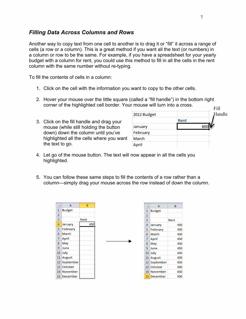
Filling Data Across Columns and Rows Another way to copy text from one cell to another is to drag it or “fill” it across a range of cells (a row or a column). This is a great method if you want all the text (or numbers) in a column or row to be the same. For example, if you have a spreadsheet for your yearly budget with a column for rent, you could use this method to fill in all the cells in the rent column with the same number without re-typing. To fill the contents of cells in a column:

1. Click on the cell with the information you want to copy to the other cells.

2. Hover your mouse over the little square (called a “fill handle”) in the bottom right corner of the highlighted cell border. Your mouse will turn into a cross.

3. Click on the fill handle and drag your mouse (while still holding the button down) down the column until you’ve highlighted all the cells where you want the text to go.

4. Let go of the mouse button. The text will now appear in all the cells you highlighted.

5. You can follow these same steps to fill the contents of a row rather than a column—simply drag your mouse across the row instead of down the column.

Fill Handle

8

You can also use this technique to copy formulas across columns and rows in the spreadsheet. PRACTICE: Type January in cell A4 as shown above. Use the fill handle and drag down to row 15. This should populate February through December in those cells. In cell B4, type 450. Use the fill handle and drag down to row 15. Now the amount will be filled in for the other months as well.

MORE ABOUT FORMATTING CELLS In the Excel Basics class, we mentioned briefly that you can format the way your data is represented within each cell. Now we’re going to look at some of these formatting options in more detail so you can get more practice with them. Remember, changes you make to cell formatting will only apply to cells that you have selected (highlighted by clicking on them). Numbers The numbers you enter in a spreadsheet can represent many different things–dates, times, percentages, currency, etc. Depending on what you want to represent, you will want your number to appear a certain way. To change the appearance of a number:

1. Select a cell or range of cells by highlighting them.

2. On the HOME tab, click on the downward-pointing arrow next to “General” in the Number group.

3. Choose an option from the list that appears (for example, “Number” or “Currency”). OR

4. If you don’t see an option that you want, click on More Number Formats at the bottom of the list.

5. A new dialog box will appear where you can choose a category.

6. Depending on the category you choose, you will see different options you can set for how you want the number to look. When you are finished changing these settings, click OK.

9

For example, if you choose Number from the category list, you will have options to change the number of places after the decimal point, choose whether or not you want a comma in numbers over 1,000, and choose how you want negative numbers to look. If you choose Date from the category list, you can choose whether you want the date to display as 3/14/2001, or 14-Mar-01, or March 14, 2001 (as well as other choices). PRACTICE: Click the “B” at the top of the rent column to highlight the entire column. On the HOME tab, click on the downward-pointing arrow next to “General” in the Number group and select Currency. The amounts should now look like this: Alignment Aligning text within a cell refers to where the text is positioned inside the cell (left, right, center, top, bottom). Excel allows you to position your text wherever you want inside a cell. To format the alignment of text:

1. Click on the Format button from the Cells group on the HOME tab.

2. Click on Format Cells from the bottom of the menu that appears.

3. Click on the Alignment tab.

4. Choose where you want your text positioned horizontally from the Horizontal drop-down box (all the way to the left side of the cell, all the way to the right, in the center, etc.).

5. Choose where you want your text positioned vertically from the Vertical drop-down box (top, center, bottom, etc.).

Other options on the Alignment tab include the check boxes under Text Control. These options are useful if you have text that is too long to fit inside a single cell. Wrap text will wrap the text within a cell so that it appears on multiple lines if it is longer than the

10

column width. This will also make the cell taller. Shrink to fit will shrink the contents of a cell so that it all appears within a cell (the more text there is, the smaller it will appear). Merge cells will remove the border between two or more cells so it becomes one extra-long cell to fit the text.

(Similar to the Merge cells command, the Merge and Center button on the Home tab will merge several cells together and center the text across the merged cells. This is a great tool for creating a title for your spreadsheet or creating a heading that spans across multiple columns.) Note that if you select multiple cells with data in it, using Merge or Merge & Center will cause you to lose all data except that which is in the upper left cell. You might also want to change the orientation of the text, or the angle of the text within the cell. You can choose to have your text appear vertically, horizontally, or any angle in between. This might be useful for column headings. To change the orientation, click on the red dot in the diagram under Orientation on the Alignment tab and drag it until the text appears at the angle you want. Borders As you probably know, borders are the lines around each cell. By default, the borders that appear on the screen are a light gray color. You might want to make the borders more visible or even make certain cells stand out by making the borders thicker or have a different line style than other cells. Also, it is important to note that when you print a spreadsheet, you will not see any lines between cells unless you have specified that you want a border around them. Even though you can see the light gray lines between cells on the screen, these will not print on the page. Excel will only print borders that you have added manually. To format cell borders:

1. Select a cell or group of cells by highlighting them.

2. Click on the Borders button from the Font group on the HOME tab.

3. Choose an option from the menu that appears. You will have options about which sides of the cell you want borders for, what line style you want,

11

and the line color. OR

4. If you want other options, click on the More Borders option from the bottom of the menu that appears. A dialog box will appear where you can select options for formatting borders. You don’t have to have a border around the entire cell – you can choose to just have the top and bottom border of the cell, for example.

PRACTICE: Select cells A4 through E15 on your spreadsheet. Click on the downward-facing arrow next to the Borders button from the Font group on the HOME tab. Select “Top and Thick Bottom Border.” Your spreadsheet should now look similar to the following:

Colors and Patterns Within a spreadsheet, there may be certain cells that you want to stand out, like the headings for rows and columns. One way to emphasize cells is to give them a background color or pattern. To add colors and patterns to cells:

12

1. Select a cell or group of cells by highlighting them.

2. Click on the Format button from the Cells group on the Home tab.

3. Click on Format Cells from the bottom of the menu that appears.

4. Click on the Fill tab.

5. If desired, choose a color from the color options.

6. If desired, choose a pattern from the drop-down box. You will see a preview of what you’ve chosen in the Sample area of the dialog box.

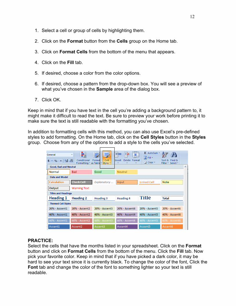
7. Click OK. Keep in mind that if you have text in the cell you’re adding a background pattern to, it might make it difficult to read the text. Be sure to preview your work before printing it to make sure the text is still readable with the formatting you’ve chosen. In addition to formatting cells with this method, you can also use Excel’s pre-defined styles to add formatting. On the Home tab, click on the Cell Styles button in the Styles group. Choose from any of the options to add a style to the cells you’ve selected.

PRACTICE: Select the cells that have the months listed in your spreadsheet. Click on the Format button and click on Format Cells from the bottom of the menu. Click the Fill tab. Now pick your favorite color. Keep in mind that if you have picked a dark color, it may be hard to see your text since it is currently black. To change the color of the font, Click the Font tab and change the color of the font to something lighter so your text is still readable.

13

MORE PRACTICE WITH FORMULAS AND FUNCTIONS In the previous class, we talked a little bit about Excel’s ability to calculate equations and formulas. This is a very powerful tool, and getting a formula to work correctly can be complicated and challenging, so let’s practice creating formulas a little bit more.

Functions You don’t have to write all of your equations from scratch–Excel has many commonly used ones already programmed for you. These are called functions, and we started looking at them in the Introduction to Excel class. Let’s practice using more of Excel’s functions. In the previous class, we looked at the AutoSum function, which adds together the numbers in a group of cells. Another common function is the Average function, which finds the average of a range of numbers. Using this function is similar to the way you used the AutoSum function.

1. Select the cell where you want the answer to the Average function to appear by clicking on it.

2. Click on the downward arrow next to the AutoSum button on the Home tab.

3. Click on Average from the list that appears (see picture to the right).

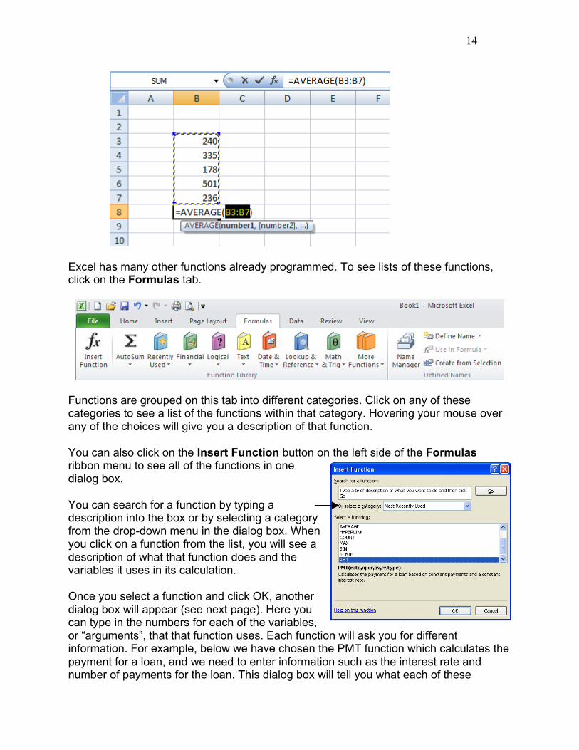
4. Excel will create the equation for you and choose the range of cells it thinks you want to find the average of. The border around this range of cells will turn into “marching ants”. If these are not the cells you want to use, you can edit the function by typing the desired cell names in the formula bar.

Remember, the range of cells is represented as (FirstCell:LastCell) where FirstCell and LastCell are replaced with the cell names (here, B3 and B7). The : between the cell names means that all cells in between the first and last will be included in the calculation.

14

Excel has many other functions already programmed. To see lists of these functions, click on the Formulas tab.

Functions are grouped on this tab into different categories. Click on any of these categories to see a list of the functions within that category. Hovering your mouse over any of the choices will give you a description of that function. You can also click on the Insert Function button on the left side of the Formulas ribbon menu to see all of the functions in one dialog box. You can search for a function by typing a description into the box or by selecting a category from the drop-down menu in the dialog box. When you click on a function from the list, you will see a description of what that function does and the variables it uses in its calculation. Once you select a function and click OK, another dialog box will appear (see next page). Here you can type in the numbers for each of the variables, or “arguments”, that that function uses. Each function will ask you for different information. For example, below we have chosen the PMT function which calculates the payment for a loan, and we need to enter information such as the interest rate and number of payments for the loan. This dialog box will tell you what each of these

15

arguments mean, and you can click on “Help on this function” at the bottom of the dialog box for more help. Using functions can often be challenging, so don’t be afraid to make a mistake the first few times.

Creating Charts and Graphs In Excel, there are also ways to represent your data in chart or graphical forms. To create a chart or graph, select the Insert tab from the Ribbon Menu bar. In the middle of this new menu, you will see a “Charts” box.

1. Select the range of data to be represented in the chart or graph. Click on your spreadsheet and select the data to be represented using the same method that you used to select data in the sorting exercise.

2. Select the type of chart or graph you wish to create (for our example, we’ll choose a pie chart).

3. Once you have created your graph, you can now “customize” it by giving it a title

and labeling different parts. You can also make certain design decisions

Variables used by this function and description of what it calculates

16

regarding the appearance of your graph or chart by choosing the different elements under the Design tab that appears on the Ribbon Menu bar.

4. Finally, you will need to decide if your chart should be pasted on to the existing spreadsheet or if it should be pasted on to a brand new sheet. On the very right side of the Ribbon Menu bar, select Move Chart.

Once the chart or graph has been created and you realize a mistake has been made or it did not turn out the way you wanted it to, simply click on the chart or graph and hit the Backspace key on your keyboard to delete it from your spreadsheet. Don’t be afraid to go back and try again! PRACTICE: Create a new sheet called “Sheet2” in your workbook and input the data to the right. Select the cells that contain your data (A1 through B7). From the Insert ribbon, in the Charts section, select Pie. Now choose a 2D pie chart. We now have a pie chart showing the percentages of each individual item. If you hover over each slice of the “pie”, you will see both a value and percentage displayed. Change the amount of gas to $100 and note the pie chart will update to show the new percentages.

17

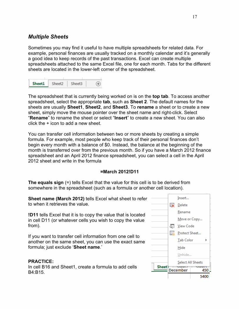
Multiple Sheets Sometimes you may find it useful to have multiple spreadsheets for related data. For example, personal finances are usually tracked on a monthly calendar and it’s generally a good idea to keep records of the past transactions. Excel can create multiple spreadsheets attached to the same Excel file, one for each month. Tabs for the different sheets are located in the lower-left corner of the spreadsheet.

The spreadsheet that is currently being worked on is on the top tab. To access another spreadsheet, select the appropriate tab, such as Sheet 2. The default names for the sheets are usually Sheet1, Sheet2, and Sheet3. To rename a sheet or to create a new sheet, simply move the mouse pointer over the sheet name and right-click. Select “Rename” to rename the sheet or select “Insert” to create a new sheet. You can also click the + icon to add a new sheet. You can transfer cell information between two or more sheets by creating a simple formula. For example, most people who keep track of their personal finances don’t begin every month with a balance of $0. Instead, the balance at the beginning of the month is transferred over from the previous month. So if you have a March 2012 finance spreadsheet and an April 2012 finance spreadsheet, you can select a cell in the April 2012 sheet and write in the formula

=March 2012!D11 The equals sign (=) tells Excel that the value for this cell is to be derived from somewhere in the spreadsheet (such as a formula or another cell location). Sheet name (March 2012) tells Excel what sheet to refer to when it retrieves the value. !D11 tells Excel that it is to copy the value that is located in cell D11 (or whatever cells you wish to copy the value from). If you want to transfer cell information from one cell to another on the same sheet, you can use the exact same formula; just exclude ‘Sheet name.’

PRACTICE: In cell B16 and Sheet1, create a formula to add cells B4:B15.

18

Rename Sheet1 to BudgetA and rename Sheet2 to BudgetB.

Go to the BudgetB sheet and in cell A1, enter =BudgetA!B16 and press Enter. Cell A1 should now show 5400 and the Function Bar will reflect the reference to BudgetA. Go back to the BudgetA sheet and change some of the rent values. Not only will that change the total in cell B16, it will also change the total on the BudgetB sheet.

CLOSING MICROSOFT EXCEL Saving Spreadsheets When you finish your spreadsheet and want to leave the computer, it is important to save your work, even if you are printing a hard copy. To save your work in Excel, it is essential to know WHAT you are trying to save and WHERE you are trying to save it. Click on the File Tab, then click “Save As” to get started. You can change the filename that Excel has chosen just by typing a new one in the “File name” box at the bottom of the window that appears. The My Documents folder on your computer’s hard drive is a good place to store your documents. A blank CD or a USB jump drive are great portable storage options and can

contain a LOT of data. Excel will automatically save your document with the suffix “.xlsx”–this is simply a tag that lets Excel know that your work is specific to this program and what version it is in. You do not have to type it–just highlight what is there (default is “Book1”) and write a new file name. You may also chose to save it in an older format so that it can be opened with older versions of Excel.

19

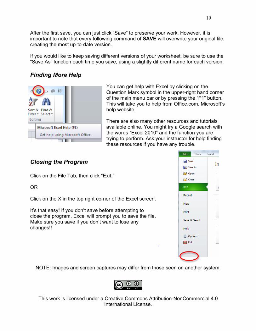
After the first save, you can just click “Save” to preserve your work. However, it is important to note that every following command of SAVE will overwrite your original file, creating the most up-to-date version. If you would like to keep saving different versions of your worksheet, be sure to use the “Save As” function each time you save, using a slightly different name for each version. Finding More Help

You can get help with Excel by clicking on the Question Mark symbol in the upper-right hand corner of the main menu bar or by pressing the “F1” button. This will take you to help from Office.com, Microsoft’s help website. There are also many other resources and tutorials available online. You might try a Google search with the words “Excel 2010” and the function you are trying to perform. Ask your instructor for help finding these resources if you have any trouble.

Closing the Program Click on the File Tab, then click “Exit.” OR Click on the X in the top right corner of the Excel screen. It’s that easy! If you don’t save before attempting to close the program, Excel will prompt you to save the file. Make sure you save if you don’t want to lose any changes!!

NOTE: Images and screen captures may differ from those seen on another system.

This work is licensed under a Creative Commons Attribution-NonCommercial 4.0 International License.