Does the Real Interest Parity Hypothesis Hold? Evidence for

Developed and Emerging Markets

Alex Luiz Ferreira Miguel A. León-Ledesma

Department of Economics, University of Kent

August 2003

Abstract: Evidence is presented on the Real Interest Parity Hypothesis for a set of emerging and developed countries. This is done by carrying out a set of unit-root tests on the real interest differentials with respect to Germany and the US. Our results support the hypothesis of a rapid reversion towards a zero differential for developed countries and towards a positive one for emerging markets. An important result is that this adjustment tends to be highly asymmetric and markedly different for developed and emerging countries. Our evidence reveals a high degree of market integration for developed countries and highlights the importance of risk premia for emerging markets. Keywords: Real Interest Rate Differentials, Market Integration, Unit Roots, Asymmetric adjustment. JEL Classification Numbers: F32, F21, C22. Acknowledgements: We would like to thank, without implicating, Yunus Aksoy, Alan Carruth and Ole Rummel for helpful comments on earlier drafts of this paper. The paper also benefited from comments of participants at the EcoMod2003 Conference in Istanbul, July 3-5, 2003. Ferreira acknowledges financial support from the Conselho Nacional de Desenvolvemento Cientifico e Tecnológico (CNPq) of Brazil. Address for correspondence: Miguel A. León-Ledesma, Department of Economics, Keynes College, University of Kent, Canterbury, Kent, CT2 7NP, UK. Phone: +00 + 44 (0)1227 823026. Fax: +00 +44 (0)1227 827850. Email: M.A.Leon-Ledesma@kent.ac.uk

2

Does the Real Interest Parity Hypothesis Hold? Evidence for

Developed and Emerging Markets

1. Introduction

The Real Interest Rate Parity Hypothesis (RIPH) states that if agents make

their forecasts using rational expectations, and arbitrage forces are free to act in the

goods and assets markets, then real interest rates between countries will equalise.

Several studies have tested this hypothesis since the pioneer papers of Mishkin (1984)

and Cumby and Obstfeld (1984). However, the empirical literature does not offer a

conclusive answer regarding the existence of real interest rate differentials (rids). For

instance, the evidence found by Gagnon and Unferth (1995), Ong et al. (1999), Evans

et al. (1994), Chinn and Frankel (1995), Alexakis et al. (1997), Cavaglia (1992),

Phylaktis (1999), Awad and Goodwin (1998), Frankel and Okongwu (1995), Fujii and

Chinn (2000) and Jorion (1996) is mixed. These authors tend to conclude that rids are

relatively short-lived and mean-reverting but different from zero in the long-run.

The importance of this hypothesis stems from the fact that empirical evidence

can be interpreted as a measure of international integration in goods and assets

markets. This is particularly emphasised in Chinn and Frankel (1995), Phylaktis

(1999), Alexakis et al. (1997), Awad and Goodwin (1998), Obstfeld and Taylor

(2002) and Mancuso et al (2002). This is because the RIPH is based on the existence

of frictionless markets. It follows that a test of the real interest rate parity is a test of

the degree of market integration.

The paper presents further evidence on the RIPH for a sample of small open-

economies in relation to the USA and Germany. We aim to unveil whether some of

our set of small open economies have been experiencing ex post real interest rate

differentials (rid(s) hereafter) in relation to larger ones. We do so by carrying out a set

3

of unit root tests that will characterise the dynamic behaviour of rids. There are few

papers in the economic literature investigating the real interest rate parity hypothesis

through unit root tests on rids. The main examples are Meese and Rogoff (1988),

Edison and Pauls (1993) and Obstfeld and Taylor (2002). Our study complements

these authors in three main directions. First, we make use of more powerful unit root

tests and take structural changes into account. Second, in line with recent theoretical

and empirical models of capital flows, we simultaneously test for the existence of

asymmetries and unit roots in the behaviour of rids.1 Third, we focus both on

developed and emerging market economies during a period with a high degree of

financial and goods market liberalisation, which is in accordance with the

assumptions underlying the real interest rate parity hypothesis. This will allow us to

compare the behaviour of rids in developed and emerging markets. Our findings show

that rids are in general quickly mean reverting, with a positive mean for emerging

markets and zero or close to zero for developed ones. We also show that rids show

strong features of asymmetry, but the behaviour for emerging and developed markets

is substantially different.

The paper is organised as follows. In the Section 2 we give some theoretical

background and describe the methodology involved in the tests; in Section 3 we

describe the data; Section 4 presents the results of unit root tests; Section 5 presents

the results of the asymmetry tests and Section 6 concludes.

2. Theoretical background and methodology

As far as agents make their forecasts using rational expectations [represented

in equation (3) below], arbitrage forces in the goods and assets markets ensure that the

1 See, for instance, Kraay (2003), Pakko (2000) and the review of Stiglitz (1999). Asymmetries could also arise in the adjustment of prices due to goods market frictions arising from transaction costs as in Obstfeld and Rogoff (2000).

4

real interest rates parity hypothesis hold. Arbitrage forces are formalised by the

uncovered interest rate parity (UIRP) and the relative purchasing power parity (PPP)

conditions stated in equations (1) and (2), respectively:

* et t ti i ds− = (1)

*t t tds π π= − (2)

et t tds ds ε= + (3)

Where i is the domestic interest rate and i* is the exogenously determined foreign

interest rate that matures at time t. The exchange rate is the domestic price of the

foreign currency and is represented by St; the expected rate of depreciation of the

exchange rate is 1

1e

e tt

t

SdsS −

= − , with the superscript e denoting expected values. The

rates of domestic and foreign inflation are tπ and *tπ respectively; and d is the first

difference of the logarithm. tε is a disturbance term that exhibits the classical

properties, i.e. 2 is iid N(0, )t εε σ and 2εσ represents its variance. Lower case variables,

except interest rates, here and elsewhere represent natural logarithms.

If PPP holds, we can substitute equation (2) into (3) and the result into (1),

which yields:

* *t t t t ti i π π ε− = − + . (4)

Equation (4) can also be rewritten as

* *( ) ( )t t t t ti i ridπ π ε− − − = = (5)

Since 2 are iid N(0, )t εε σ , the expected value of the rid is zero.

Now consider that ridt follows a more general stochastic process:

0 1 1t t trid a a rid ε−= + + (6)

5

Assuming that 0rid is a deterministic initial condition, the solution to the difference

equation above is:

10 1

1 0 101

(1 )(1 )

t tt i

t t ii

a arid a rid aa

ε−

−=

−= + +

− ∑ . (7)

If 1 1a < and allowing t to increase to infinity, the limit towards which the rid

converges in the long run is equal to:

0

1

lim1tt

arida→∞

=−

(8)

Taking expectations of equation (8) and considering the RIPH, we have

00

1

( ) 0 01t

aE rid aa

= = ⇔ =−

(9)

It follows from equation (5) that if UIRP, PPP and rational expectations hold,

the rid is equal to the unforeseeable disturbance term related to the forecast of

exchange rate depreciation2. From equation (9) we observe that a rid does not exist in

the long run because its unconditional mean, or expected value, is equal to zero. The

problem is to verify whether shocks to the series of rids dissipate and the series

returns to its long-run zero mean level. This objective can be accomplished by

performing unit root tests on the series of rids.

We can represent the model of equation (6) as a pth-order autoregressive

process,

1 12

0

p

t t i t i ti

rid a rid ridψ β ε− − +=

∆ = + + ∆ +∑ , (10)

where,

1

1q

ii

aψ=

= −∑ . (11)

2 In fact the ex post rid can also be derived from the Fisher (1930) equation. In that case the ex post rid equals the ex ante rid plus a disturbance term related to the inflation forecast, given that rational expectations is assumed [Mishkin (1984)].

6

The following possibilities arise from the estimation of this ADF-type

equation (10):

0 ψ > (12)

0 ψ = (13)

00 and 0aψ < = (14)

00 and 0aψ < ≠ (15)

Inequality (12) represents the case in which the parameter ψ is statistically

greater than zero. The path of rids in this case would be explosive and the series

would not converge to any mean in the long run. In (13) the series contains a unit root

and rids follow a random walk with shocks affecting the variable on a permanent

basis. In cases (14) and (15) the estimated parameter (ψ) is such that1

1q

ii

a=

<∑ .

Deviations from the mean are temporary and the estimated root provides information

on whether the rid is short-lived or persistent. In (14) the rid follows a stationary

process and converges to a zero mean. The RIPH holds and the speed of adjustment of

the rid to its equilibrium level is a measure of the degree of persistence. In (15) rids

converge to a mean that is different from zero. In summary, short-lived rids are

consistent with the RIPH because the series rapidly reverts to zero. Persistent rids that

converge to a constant mean that is equal to zero are also consistent with the RIPH,

since shocks eventually dissipate. The existence of a mean different from zero may

arise theoretically from a country specific risk premium. However, random walks,

permanent or explosive rids are inconsistent with the real interest rate parity

hypothesis.

Three usual problems with standard unit root tests, such as the ADF, arise.

First, it is well known that the power of these tests tends to be very low, leading to

over-acceptance of the null of a unit root. The low power problem is magnified for

7

small samples because a stationary series could be drifting away from its long-run

equilibrium level in the short-run. Another serious problem of unit root tests is not

considering the existence of structural breaks in the series. When there are structural

changes, the standard tests are biased towards the non-rejection of a unit root [Perron

(1989)]. Finally, since the work of Neftci (1984), it has been increasingly recognised

that macroeconomic time series show strong asymmetry over the business cycle. If

asymmetry is present in rids, linear unit-root tests will suffer from a loss of power.3

Several tests have been put forward to alleviate these problems. Kwiatkowski

et al (1992) use the LM statistic to test the null hypothesis of stationarity (KPSS test).

The time-series in their model is written as the sum of a deterministic trend, a random

walk and a stationary error. The null corresponds to the hypothesis that the variance of

the random walk equals zero, in other words, the variance of the error is constant.

When the series has an unknown mean or linear trend, the tests suggested by Elliot et

al (1996) (ERS test hereafter) and Elliot (1999) are recommended. These tests use

information contained in the variance of the series to construct a test statistic (DF-

GLS and ADF-GLS) that has more asymptotic power than the standard ones. The

initial condition is assumed to be zero in the ERS test while it is drawn from its

unconditional distribution in Elliot (1999). Regarding the existence of structural

breaks, Perron (1997) developed a procedure to test for unit-roots that endogenously

searches for structural breaks in the series using two methods. In the first method, the

break date is chosen to be the one in which the t-statistic for testing the null

hypothesis of a unit root is smallest among all possible break points. In the second

method, the break point corresponds to a maximum of the absolute value of the t-

statistic on the parameter associated with the change in the intercept. We will make

use of both when testing the RIPH assuming symmetric behaviour of the rid to

3 See Enders and Granger (1998). They also show evidence of asymmetry in the adjustment of the term structure of interest rates.

8

positive and negative shocks. Later on we relax this assumption and apply the tests

proposed by Caner and Hansen (2001) that allows for testing unit roots and

asymmetry using threshold autoregressive methods. This is because some theoretical

and empirical models of credit markets with imperfect information point out to

possible asymmetric behaviour of rids as changes in interest rates may influence

subjective risk perceptions by creditors. If the series are asymmetric, the power of

unit-root tests will improve. The pattern of asymmetry showed by rids is also a

relevant issue in itself, especially when we compare different countries.

While there is a substantial number of papers testing unit roots in nominal

interest rates, inflation and even real interest rates, few studies are concerned with rids

especially when the objective is to test the real interest rate parity hypothesis. Meese

and Rogoff (1988) performed unit root tests in the series of rids of the US, UK, Japan

and Germany over the period 1974M2 to 1986M3. They could not reject the

hypothesis that there is a unit root in the series of long term real interest rate

differentials, but not in short-term differentials. In fact, they found that both nominal

and real short-term interest rate differentials appear to be stationary in levels. Along

the same line of Meese and Rogoff (1988), Edison and Pauls (1993) performed ADF-

tests on rids using quarterly observations from 1974 to 1990 for the G-10 countries.

They could not reject the unit root hypothesis.

Obstfeld and Taylor (2002) questioned why Meese and Rogoff (1988) Edison

and Pauls (1993) and McDonald and Nagayasu (2000) could not reject the unit root

hypothesis given the increasing globalisation of capital markets “…if capital is

perfectly mobile, this dooms to failure any attempts to manipulate local asset prices to

make them deviate from global prices, including the most critical macroeconomic

asset price, the interest rate” (pp.17). In their view, the failure to reject the null stems

from the fact that these authors focused attention on the recent float, had shorter

9

samples, and used tests of low power such as the ADF test. The sample used by

Obstfeld and Taylor (2002) includes rids of three countries relative to the USA (UK,

France and Germany) from 1870 to 2000. Their results, using standard ADF and

Elliott (1999) tests, show that the hypothesis of a unit root can be rejected at the 1%

level in all periods except for the recent float: “The most striking impression

conveyed by the figure is that differentials have varied widely over time, but have

stayed relatively close to a zero mean. That is the series appear to have been

stationary over the very long run, and even in shorter sub periods.” (pp.26). By

splitting the sample of the recent float in two sub periods (1974-1986 and 1986-2000)

they found that the evidence against a unit root is stronger over the second sub period.

3. Data

The countries chosen for our tests can be split into three groups. The first one

comprises some small open-economies of emerging markets: Argentina, Brazil, Chile,

Mexico and Turkey. The second group is composed of small open-economies of

developed countries: France, Italy, Spain and the UK. Finally, the third group is the

one with the countries used as the reference large economies for the calculation of

rids: Germany and USA. The period of the tests corresponds to the interval that spans

from 1995M3 to 2002M5, with the exceptions of Argentina, for which we have

calculated rids until 2002M3, and Chile and the UK, with rids calculated until

2002M4. The shorter period of the former countries is due to data availability. This

heterogeneous sample of countries allows inter-group comparisons and the detection

of similar patterns between them.

10

Our sample period starts in the mid 90s because harmonised data for the

construction of the rids for some of our countries did not exist before this period.4 An

advantage of using this period is that after the mid-90s most of the countries had

liberalised capital markets and had advanced substantially in their trade liberalisation

process. As shown previously, the RIPH is based on the assumptions of frictionless

goods ands assets’ markets. If there are restrictions to trade in these markets, arbitrage

would be constrained and different outcomes from those predicted by the RIPH may

arise. The process of trade and financial liberalisation happened during different

periods for the countries in our sample. Trade liberalisation in developing economies

was carried out in the late 1980’s and early 1990’s5. Financial liberalisation happened

almost simultaneously6. Hence, we focus on the second half of the 1990’s using data

available until the most recent period.

The ex post real interest rate is defined as

t t tr i π= − , (16)

where it is the nominal interest rate earned on a one-period bond or deposit

that matures at time t, i.e., it is the nominal return from holding the one-period bond

from t-1 to t; π is the actual (or ex post) inflation from t-1 to t. Data on interest rates

was obtained from IMF’s International Financial Statistics (IFS). Among the several

categories of interest rates available in the IFS database, we considered the Treasury

Bill Rate as being the most appropriate for the tests. In practice, there is no unique

variable that international arbitrageurs use to compare their prospective returns at

home and abroad. However, the Treasury Bill Rate is available in domestic markets to

4 We decided to test the RIPH for the same period for all countries to allow for comparison of the results. 5 See UNCTAD (1999). 6 Edwards (2001), among others, acknowledged the difficulty in measuring the “true” degree of capital mobility and thus the starting period of the financial liberalisation. In spite of this difficulty, however, it is recognised that there has been a marked increase in the flows of capital across countries especially during the nineties.

11

international arbitrageurs and has a fixed maturity. For these reasons, we have chosen

to use the Treasury Bill Rates for Brazil, Mexico, Italy, Spain, UK, USA and

Germany. We use deposit rates for Argentina, Chile and Turkey because the

availability of data on Treasury Bill Rate was limited for these countries. This is the

only other short-term interest rate available with a specified maturity. As regards the

choice of maturity, as stated by the liquidity premium theory, investors tend to prefer

bonds with short-term maturities rather than bonds with longer-term maturities, since

the former bear less interest-rate risk. Forecast errors of exchange rate changes are

also more likely to increase as time increases. Because we are interested in verifying

the degree to which real interest rates are different across countries, we have decided

to use short term rates instead of long-term ones in order to avoid a greater influence

of risk premium and forecast errors in the composition of rids.

Hence, in order to calculate rids we transformed the annualised monthly

interest rate into a compounded quarterly rate; the real interest rate was then

calculated by subtracting the quarter-on-quarter inflation rate from the compounded

nominal interest rate of three months. The inflation rate is the rate of growth of the

Consumer Price Index (CPI).7 Our choice of interest rate and inflation is in

accordance with the data used by the majority of the authors testing the UIRP. For

instance, Mishkin (1984), Knot and de Haan (1998), Nakagawa (2002), Phylaktis

(1999), Alexakis et. al. (1997) used interest rates that included either the 3-month

Treasury Bill or the 3-month deposit rate. The great majority of authors also used the

CPI as the appropriate deflator.

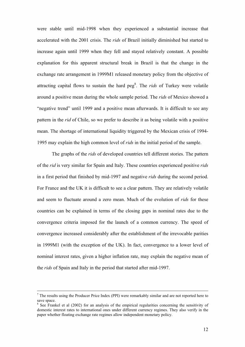
Figure 1 plots the different rids with respect to Germany and the US. With the

exception of Chile, rids were high in all developing countries at the beginning of the

sample period and behaved differently afterwards. The rids of Argentina, for example,

12

were stable until mid-1998 when they experienced a substantial increase that

accelerated with the 2001 crisis. The rids of Brazil initially diminished but started to

increase again until 1999 when they fell and stayed relatively constant. A possible

explanation for this apparent structural break in Brazil is that the change in the

exchange rate arrangement in 1999M1 released monetary policy from the objective of

attracting capital flows to sustain the hard peg8. The rids of Turkey were volatile

around a positive mean during the whole sample period. The rids of Mexico showed a

“negative trend” until 1999 and a positive mean afterwards. It is difficult to see any

pattern in the rid of Chile, so we prefer to describe it as being volatile with a positive

mean. The shortage of international liquidity triggered by the Mexican crisis of 1994-

1995 may explain the high common level of rids in the initial period of the sample.

The graphs of the rids of developed countries tell different stories. The pattern

of the rid is very similar for Spain and Italy. These countries experienced positive rids

in a first period that finished by mid-1997 and negative rids during the second period.

For France and the UK it is difficult to see a clear pattern. They are relatively volatile

and seem to fluctuate around a zero mean. Much of the evolution of rids for these

countries can be explained in terms of the closing gaps in nominal rates due to the

convergence criteria imposed for the launch of a common currency. The speed of

convergence increased considerably after the establishment of the irrevocable parities

in 1999M1 (with the exception of the UK). In fact, convergence to a lower level of

nominal interest rates, given a higher inflation rate, may explain the negative mean of

the rids of Spain and Italy in the period that started after mid-1997.

7 The results using the Producer Price Index (PPI) were remarkably similar and are not reported here to save space. 8 See Frankel et al (2002) for an analysis of the empirical regularities concerning the sensitivity of domestic interest rates to international ones under different currency regimes. They also verify in the paper whether floating exchange rate regimes allow independent monetary policy.

13

4. Unit root tests

The results of ADF tests are reported in Table 1. We found the optimal

augmentation lags by using a sequential general-to-specific criteria. The results show

that we can reject the hypothesis of a unit root only for Brazil, Mexico, Turkey and

UK(Ger).9 It must be stressed, however, that our test statistics were very sensitive to

the number of lags, which means that inaccuracy in the lag selection may have led to

biased conclusions. Increasing the number of lags of Brazil from 3 to 5, or in the case

of Mexico from 1 to 5, for example, imply the non rejection of the null hypothesis of a

unit root. Nonetheless, as briefly discussed in section II, failure to reject the unit root

is likely to be explained by the low power of ADF tests. Hence, we performed the

already mentioned more powerful tests. As we can see in Table 1, the results using

ERS (1996) were slightly different. Using the same number of lags chosen for the

ADF tests, we could reject the unit root hypothesis not only for Brazil, Mexico and

Turkey but also for the rid of Chile-US. The findings of the tests using the method

proposed by Elliot (1999) were very similar to that of ERS (1996), the only difference

is that we could also reject the null of a unit root for the rid of UK(Ger) which we

were already able to reject using ADF tests. The KPSS test allowed us to accept the

hypothesis of stationarity for most countries of the sample. Apart from the countries

mentioned before, we could not reject the hypothesis of level-stationary for the rids of

Argentina, France(US) and Chile(Ger) but not for Brazil. We could also not reject the

null of stationary for the rid of the UK and US(Ger).

Although these methods provide more powerful alternatives to the ADF test,

they do not take into account structural breaks. The plots of rids in Figure 1 reveal

that many of these series may contain a break in their mean. This is especially so for

9 When we refer to the rid of a country 1 with respect to country 2 we will use the notation country1(country2). So the rid of, for instance, Turkey with respect to Germany would be Turkey(Ger). When we mention only “Turkey” we are referring to both rids.

14

Argentina, Mexico, Brazil, Italy and Spain.10 For this reason we applied Perron’s

(1997) tests assuming that the series contain an innovational outlier with a change in

the intercept. This model can be represented as

10 1 1( )

p

i t i ti

t t b t t ridrid a DU D T a rid β εθ λ −=

− ∆ += + + + + ∑ , (17)

where Tb denotes the break date; 1( ) and ( ) 1( 1)t b b t bDU t T D T t T= > = = + . The test is

performed using the t-statistic for the null hypothesis that a1=1. The results of this test

are reported in Table 2.

We were able to reject the unit root for Brazil, Chile, Mexico, Turkey,

Italy(Ger), Spain(Ger) and UK(Ger) using the date break suggested by the first

method. The unit root hypothesis was also rejected for Mexico(US), Turkey, Italy and

Spain(Ger) using the date break of the second method. Nevertheless, we could not

find evidence of non-stationarity for the rids of Spain(US) in any of the tests. We

suspect that systematic forecast errors due to excessive credibility in the convergence

to low inflation levels could explain the unit root behaviour of the rid of Spain(US).

The date breaks retrieved by the tests suggest that the Asian crisis (starting in

mid 1997) impacted on the rids of Chile and, less likely, the rids of France(US), Italy

and Spain. Another explanation for the break dates of the latter countries is that rids

were affected by the Stability and Growth Pact signed by the European Council in

1997M6 and the prospect of the establishment of the European Central Bank (ECB),

that officially took place in 1998M6. The Mexican crisis (1994M12) appears to have

impacted on the rids of Brazil, as can be seen in the date break found by the first

method. The Russian crisis (mid 1998) may have had an effect on the rids of Mexico

and Chile(US). The Brazilian crisis (1999M1) is captured by the date break of the rids

of that country retrieved by the second method. The Brazilian crisis probably

10 This is further confirmed by plots of the recursive Chow tests of the AR parameter, not reported here but available on request.

15

impacted the rids of Argentina as can be seen in the date break suggested by the

second method. The free float of the Peso in Argentina 2002M1 is reflected in the

date break of the first method. The results also indicate that the Turkish crisis, which

culminated in 2001M2 with the free floating of the Lira, may have its origins at the

beginning of 1999.

According to our results, the irrevocable parities announced in 1999M1 for the

Euro area and the introduction of the Euro as a medium of exchange in 2002M1, have

not been reflected in the form of a structural break during the sample period. Our

results also suggest that the Asian financial crisis and/or the establishment of the

European System of Central Banks may have affected the rids of developed countries

in a structural manner.

The tests carried out also allowed us to calculate half-lives of deviations from

equilibrium and the equilibrium itself as given by equation (8). It must be stressed that

rids converge to an equilibrium level only if there is not a unit root in the series. As

previously stated, the low power of the traditional tests implies that a unit root may

not exist even if we are not able to reject the null. Hence, we decided to calculate the

half-life and equilibrium level of rids for all countries including Spain(US). The

results are reported in Table 3.

According to the estimated roots obtained with standard ADF tests, some

countries of our sample have highly persistent rids. The half-life of the rid of

Argentina, for example, varies from 3.4 to 13.1 months. In the case of Italy and Spain,

the half-life varies from 5 months to 10.3 months. The most persistent rids, according

to our results, are those of Argentina and Italy. On the other hand, the tests using the

Perron (1997) methods suggest a smaller degree of persistence for the rids of all

countries. Half-lives vary between 0 and 3.2 months, with the exception of

16

Argentina(US). Thus, when possible structural changes are taken into account, rids of

almost the whole sample are short-lived.

Estimated equilibrium levels for the rids from the ADF and Perron (1997)

equations are reported in Table 4.11 Equilibrium levels of rids are significantly

different from zero if both the intercept and estimated root are significant. Inspection

of Table 4 shows that the rids of Brazil, Chile, Mexico, Turkey, UK(Ger) and

US(Ger) converge to a mean value that is statistically different from zero. These

values were higher for Turkey, Brazil, Argentina, Mexico and Chile in descending

order. These results point out to risk premium as a likely explanation of permanent

higher levels of real interest rates. When we allowed for structural changes using the

date breaks retrieved by the first method of Perron (1997), we found that the rids of

Argentina, Brazil, Chile, Mexico, Turkey, Italy(US) and Spain converge to

equilibrium values that are statistically significant.

5. Asymmetry and unit roots

The previous unit-root tests assume that rids follow a linear representation or

linear path around a breaking trend. However, recent developments in the theory of

imperfect capital markets/imperfect information suggest that the behaviour of rids

may be asymmetric because risk perceptions may vary with changes in interest rates

themselves. The argument is summarised in Stiglitz (1999) and a similar argument put

forward in Pakko (2000).12 Given the existence of asymmetric information in

international credit markets, lenders will look at increases in interest rates as a signal

that determines their subjective probability of bankruptcy (or default). As Stiglitz

(1999) explains “[…] the probability of bankruptcy may depend on the interest rate

11 We just report equilibrium levels obtained using Perron (1997) for break search method 1, as method 2 gave similar results.

17

charged, so that beyond a point, increases in the interest rate charged actually lead to

lower expected returns” (p. 64) which relates to the idea that “The dominant effect of

large, unanticipated increases in interest rates is thus induced bankruptcies and an

increase in non-performing loans” (p. 65). The consequence of these arguments for

the RIPH is that the country risk premium may depend on changes of the interest rate

and, hence, rids would converge to different equilibrium differentials if previous

changes in rids surpass a certain threshold. This multiple equilibria idea would induce

asymmetries in the time series behavior of rids.13

Evidence on this rid nonlinearity is presented, for instance, in Mancuso et al

(2002). If asymmetries are present in the adjustment of rids, unit-root tests may lose

power and suffer size distortions unless they are incorporated in the tests (Enders and

Granger, 1998). Our approach allows us to simultaneously test for asymmetry and

unit roots in the rids series, revealing interesting features about the RIPH. If rids

behave asymmetrically, we can use the following TAR (Threshold Autoregression)

representation (Caner and Hansen, 2001):

{ } { }1 1

' '1 1 2 1

11 1

t t

p

t t t j t j tz zj

y y y ridλ λθ θ γ ζ− −− − −< ≥

=

∆ = + + ∆ +∑ , (18)

where yt-1 = (1 ridt-1), 1{.} is the indicator function that takes the value of 1 if zt-1 is

higher or lower than a threshold λ, and 0 otherwise. The variable zt is any stationary

variable that would determine the change of regime. For our purposes, we set zt = ridt

12 Some of these features are commonly introduced in models of speculative attacks with asymmetric information. The idea in the context of the 1997 South East Asian crisis is discussed in Radelet and Sachs (1998). 13 Recent papers by Nakagawa (2002) and Obstfeld and Rogoff (2000) amongst others present evidence that suggests that convergence towards PPP may be non-linear. This is usually associated with theoretical models in which market segmentation arising from various transaction costs introduce non-linearities in the adjustment of real exchange rates (RER) as in Obstfeld and Rogoff (2000). These kinds of non-linearities may also induce asymmetry in the speed of adjustment of rids to positive and negative shocks.

18

– ridt – m. That is, we assume that rids may have a different behaviour depending on

whether past changes in rids have been higher or lower than a certain threshold λ.

This is a momentum-TAR model or M-TAR as in Enders and Granger (1998). The lag

length m for the changes in rids will be data determined as will be the search for the

optimal threshold λ. Finally, the parameter vectors θ1 and θ2 can be partitioned as

11

1

µθ

ρ

=

, 22

2

µθ

ρ

=

The choice of the threshold λ could be simply made on an a priori basis, such

as setting λ = 0 or equal to the sample mean of ∆ridt. However, this would be a biased

estimate of the threshold if asymmetric adjustment exists and a subjective measure. In

order to search for the optimal threshold, we follow Chan (1993) and find λ as the

value of ∆ridt that minimises the residual sum of squares of the OLS estimation of

(18).14

In order to test for the existence of asymmetry in the adjustment under both

regimes we test the null hypothesis Ho : θ1 = θ2 on the OLS estimation of (18),

making use of the Wald statistic (W) proposed in Caner and Hansen (2001). The

RIPH would imply rejecting Ho: ρ1 = ρ2 = 0, and we also make use of two Wald

statistics (R1 and R2). Finally, we also chose m to minimise the residual sum of

squares. Given that the Wald test of asymmetry is a monotonic function of the

residual variance, we choose m as the value which maximizes the Wald test of

asymmetry.

The procedure we follow to test simultaneously for asymmetry and unit roots

implies first estimating a baseline model for the linear ADF regression to determine

the lag augmentation of the DF regression using general-to-specific techniques as in

previous sections. We then select the threshold by minimising the residual sum of

squares of (6) as mentioned earlier and fit the M-TAR model by OLS for every value

19

of m. We choose the m that minimises the residual sum of squares for all values of

m.15

Given that the asymptotic null distribution of the asymmetry test (W) is non-

standard, Caner and Hansen (2001) recommend the use of bootstrap methods to obtain

p-values. In a Monte Carlo experiment they show that the power and size of the test

does not crucially depend on whether we impose a unit-root. Hence, we obtained p-

values by carrying out 1,000 iterations of the unconstrained asymmetry test, i.e. not

imposing the existence of a unit root. Finally, the unit root hypothesis involves testing

for Ho: ρ1 = ρ2 = 0. There are two possible alternatives: H1: ρ1 < 0 and ρ2 < 0 and

1 2

2

1 2

0 0:

0 0

andH or

and

ρ ρ

ρ ρ

< = = <

The first alternative corresponds to the stationary case, whilst the second implies

stationarity in only one of the regimes, which implies overall non-stationarity but a

different behaviour from the classic unit-root. Caner and Hansen (2001) develop

asymptotic theory for the distribution of this unit-root test. However, for finite

samples they recommend the use of bootstrapping. As the distribution of the test

statistic will depend on whether or not a threshold effect exists, p-values obtained

through the bootstrap are not unique. We hence obtained the bootstrapped p-values

from 1,000 iterations under the hypothesis that the threshold is not identified (R1) and

under the hypothesis that it is identified (R2). These two tests have substantially more

power than the ADF test as threshold effects become more important. In order to

discriminate between the two alternatives in H2, Caner and Hansen (2001)

recommend looking at the t-ratios of ρ1 and ρ2.

14 In practice we eliminated the highest and lowest 10% values of ∆ridt. 15 Usually, for monthly data we take m = 1,…, 12 and for quarterly m = 1,…, 4.

20

The results are provided in Table 5 where we report the estimated threshold

(λ), the lag of the change in rids for the determination of the threshold (m), and the

estimates of the parameters of (18) in both regimes. Asymmetry appears to be a

prevalent feature in the data. We can reject the null of no asymmetry for at least one

pair of rids for all countries except Mexico and the UK. Observing the values and t-

ratios of the intercepts and autoregressive terms we can see that this asymmetry is

associated with both differences in intercepts in both regimes and asymmetric

adjustment speeds, although the former appears more frequently. As for unit roots, the

results confirm that taking asymmetry into account is important, as we can reject the

null of non-stationarity for all the countries by at least one of the R tests except for

Argentina, Italy and Spain.16 In several cases, such as US(Ger) and UK, rids appear to

be stationary when decreasing and non-stationary when increasing above the

threshold. The other way around occurs for Brazil, Chile and Turkey.

Other important features appear when observing the different behaviour of

emerging and developed markets in our sample. For France, UK and US(Ger) the

intercept is either statistically insignificantly different from zero or close to it in both

regimes. The speed of adjustment for these countries, as already mentioned, is higher

when decreasing and lower when increasing. This pattern in the speed of adjustment

is reversed for Brazil, Chile, Mexico and Turkey. Furthermore, for these countries the

intercept tends to be close to zero when the rids are growing below the threshold and

significantly higher than zero when it is rising. This positive intercept would imply

large equilibrium rids especially for Turkey and Brazil. In relation to the theoretical

models of imperfect information in credit markets, these results may seem to indicate

that large increases in interest differentials may be negatively interpreted by the

market, which in turn imposes a higher risk premium. The fact that this pattern does

not seem to arise for developed markets also supports this idea as, during this period,

16 For Italy and Spain structural breaks may be driving most of the results as seen previously.

21

none of these countries has suffered large swings of their interest rates that may have

induced this change in risk perception effect.

6. Conclusions

We have presented evidence on the Real Interest Parity Hypothesis for a set of

developed and emerging markets for the period that spans from the mid-90s until the

middle of 2002. Our results show that, despite the short time span, we were able to

find mean reversion in rids. The speed of mean reversion is high, indicating that real

differentials tend to be short lived. This is especially so if we allow for the likely

possibility of structural breaks in the series. We were able to reject the unit root

hypothesis or to accept the null of stationarity for all countries, excluding Spain

relative to the US. This evidence supports the hypothesis of a high degree of market

integration, which is consistent with financial liberalisation and the emergence of

global capital markets. The pattern of adjustment is asymmetric, that is, whenever rids

grow above or below a certain threshold they tend to behave differently. For emerging

markets adjustment is quicker when rids grow fast, while for countries such as France

and the UK adjustment is quicker when rids grow below the threshold.

Nonetheless, we found evidence supporting the existence of a positive long-

run mean in the rids of, especially, emerging markets. The long run mean of emerging

markets economies tends to be higher than for developed ones, for which it is zero or

close to zero. Our results also suggest that foreign financial crisis may have generated

structural changes in rids. Finally, we found evidence that equilibrium rids for

emerging markets are high in periods of rapid growth of the rid. All these features

point out to the existence of large risk premia for emerging markets, but not for

developed markets.

22

In general, our results support recent evidence on the RIPH for developed

countries despite the short sample of our study. It also complements this literature

with evidence from emerging markets. For these countries, the RIPH with a risk

premium component seems to be a more realistic specification. We also find that

asymmetries induced by either risk perception changes or transaction costs seem to be

an important feature when explaining real interest rates differentials.

References

Alexakis, P., Apergis, N. and Xanthakis, E. (1997). “Integration of International Capital Markets: Further Evidence from EMS and Non-EMS Membership,” Journal of International Financial Markets, Institutions and Money, (7)3, 277-287.

Awad, M. A. and Goodwin, B.K. (1998). “Dynamic Linkages Among Real Interest Rates In International Capital Markets,” Journal of International Money and Finance, (17)6, 881-907.

Caner, M. and Hansen, B.E. (2001). “Threshold Autoregressions With a Unit Root,” Econometrica, 69, 1555-1596.

Cavaglia, S. (1992). “The Persistence of Real Interest Differentials,” Journal of Monetary Economics, (29)3, 429-443.

Chan, K.S. (1993). “Consistency and Limiting Distribution of the Least Squares Estimator of a Threshold Autoregressive Model,” The Annals of Statistics, 21, 520-533.

Chinn, M.D. and Frankel, J. A. (1995). “Who Drives Real Interest Rates Around the Pacific Rim: the USA or Japan?,” Journal of International Money and Finance, (14)6, 801-821.

Cumby, R. and Obstfeld, M. (1984). “International Interest Rate and Price Level Linkages Under Flexible Exchange Rates: a Review of Recent Evidence,” in Bilson, J. and Marston, R. C., eds., Exchange Rate Theory and Practice, University of Chicago Press, Chicago.

Edison, H. J., and Pauls, B. D. (1993). “A Re-Assessment of the Relationship Between Real Exchange Rates and Real Interest Rates: 1974-1990,” Journal of Monetary Economics, 31, 165-187.

Edwards, S. (2001). “Capital Mobility and Economic Performance: Are Emerging Economies Different?”, NBER Working Paper, nº 8076.

23

Elliott, G. (1999). “Efficient Tests for a Unit Root when the Initial Observation is Drawn from its Unconditional Distribution,” International Economic Review, 40, 767-783.

Elliott, G., Rothenberg, T. J. and Stock, J.H. (1996). “Efficient Tests for an Autoregressive Unit Root,” Econometrica, 64, 813-836.

Enders, W. and Granger, C.W.J. (1998). “Unit Root Tests and Asymmetric Adjustment with an Example Using the Term Structure of Interest Rates,” Journal of Business and Economic Statistics, 16, 304-311.

Evans, L.T., Keef, S.P. and Okunev, J. (1994). “Modelling Real Interest Rates,” Journal of Banking and Finance, (18)1, 153-165.

Fisher, I. (1930). The theory of Interest. New York: McMillan, 1930.

Frankel, J. A. and Okongwu, C. (1995). “Liberalized Portfolio Capital Inflows in Emerging Markets: Sterilization, Expectations, and the Incompleteness of Interest Rate Convergence,” NBER working paper. nº 5156.

Frankel, J. A., Schmukler, S. L. and Servén L. (2002). “Global Transmission of Interest Rates: Monetary Independence and Currency Regime,” NBER Working Paper, nº 8828.

Fujii, E. and Chinn, M.D. (2000). “Fin de Siecle Real Interest Parity,” NBER Working Paper, nº. 7880.

Gagnon J.E. and Unferth, M. D. (1995). “Is There a World Real Interest Rate?,” Journal of International Money and Finance, (14)6, 845-855.

Jorion, P. (1996). “Does Real Interest Parity Hold at Longer Maturities?,” Journal of International Economics”, (40)1-2, 105-126.

Knot, K. and de Haan, J. (1995). “Interest Rate Differentials and Exchange Rate Policies in Austria, The Netherlands, and Belgium,” Journal of Banking and Finance, 363-386.

Kraay, A. (2003). “Do High Interest Rates Defend Currencies During Speculative Attacks?” Journal of International Economics, 59, 297-321.

Kwiatkowski, D., Phillips, P. C.B., Schmidt, P. and Shin, Y. (1992). “Testing the Null Hypothesis of Stationary against the Alternative of a Unit Root,” Journal of Econometrics, 54, 159-178.

MacDonald, R. and Nagayasu, J. (2000). “The Long-Run Relationship Between Real Exchange rates and Real Interest rates Differentials: A Panel Study.” IMF Staff Papers, 47, 116-128.

Mancuso, A. J., Goodwin, B. K. and Grennes, T. J. (2002). “Non-Linear Aspects of Capital Market Integration and Real Interest Rate Equalization,” International Review of Economics and Finance, forthcoming.

24

Meese, R. and Rogoff, K. (1988). “Was It Real? The Exchange Rate-Interest Differential Relation over the Modern Floating-Rate Period,” The Journal of Finance, 43, 933-948.

Mishkin, F.S. (1984). “Are Real Interest Rates Equal Across Countries? An Empirical Investigation of International Parity Conditions,” The Journal of Finance, 39, 5, 1345-1357.

Nakagawa, H. (2002). “Real Exchange Rates and Real Interest Rate Differentials: Implications of Nonlinear Adjustment in Real Exchange Rates,” Journal of Monetary Economics, 49, 629-649.

Neftci, S. N. (1984). “Are Economic Time Series Asymmetric Over the Business Cycles?” Journal of Political Economy, 85, 281-291.

Obstfeld, M. and Rogoff, K. (2000). “The Six Major Puzzles in International Finance: Is there a Common Cause?” NBER Macroeconomics Annual, 15, 339-390.

Obstfeld, M. and Talyor, A. M. (2002). “Globalization and Capital Markets,” NBER working paper, nº 8846.

Ong, L. L., Clements, K. W. and Izan, H.Y. (1999). “The World Real Interest Rate: Stochastic Index Number Perspectives,” Journal of International Money and Finance, (18)2, 225-249.

Pakko, M.R. (2000). “Do High Interest Rates Stem Capital Outflows?” Economics Letters, 67, 187-192.

Perron, P. (1989). “The Great Crash, the Oil Price Shock, and the Unit Root Hypothesis,” Econometrica, 57, 6, 1361-1401.

Perron, P. (1997). “Further Evidence on Breaking Trend Functions in Macroeconomic Variables,” Journal of Econometrics, 80, 2, 355-385.

Phylaktis, K. (1999). “Capital Market Integration in The Pacific Basin Region: an Impulse Response Analysis,” Journal of International Money and Finance (18)2, 267-287.

Radelet, S. and Sachs, J.D. (1998). “The East Asian Financial Crisis: Diagnosis, Remedies, Prospects,” Brookings Papers on Economic Activity, 1, 1-74.

Stiglitz, J.E. (1999). “Interest Rates, Risk, and Imperfect Markets: Puzzles and Policies,” Oxford Review of Economic Policy, 15(2), 59-76.

UNCTAD (1999). “Payments Deficits, Liberalization and Growth in Developing Countries.” In: Trade and Development Report. UNCTAD, Geneva.

Figure 1. Real interest rate differentials

Argentina

1995 1996 1997 1998 1999 2000 2001-1

0

1

2

3

4

5

6

7GerUS

Brazil

1995 1996 1997 1998 1999 2000 20010.0

2.5

5.0

7.5

10.0

12.5

15.0GerUS

Spain

1995 1996 1997 1998 1999 2000 2001-1.5

-1.0

-0.5

0.0

0.5

1.0

1.5

2.0USGer

Italy

1995 1996 1997 1998 1999 2000 2001-1.5

-1.0

-0.5

0.0

0.5

1.0

1.5

2.0USGer

Turkey

1995 1996 1997 1998 1999 2000 2001-5

0

5

10

15

20

25USGer

US and Germany

1995 1996 1997 1998 1999 2000 2001-1.6

-1.2

-0.8

-0.4

-0.0

0.4

0.8

1.2

1.6GerUS

Chile

1995 1996 1997 1998 1999 2000 2001-1.6

-0.8

0.0

0.8

1.6

2.4

3.2

4.0

4.8USGer

Mexico

1995 1996 1997 1998 1999 2000 2001-1.8

-0.9

0.0

0.9

1.8

2.7

3.6

4.5

5.4USGer

France

1995 1996 1997 1998 1999 2000 2001-1.0

-0.5

0.0

0.5

1.0

1.5

2.0USGer

UK

1995 1996 1997 1998 1999 2000 2001-1.5

-1.0

-0.5

0.0

0.5

1.0

1.5

2.0USGer

26

Table 1. Unit Root Tests

Country - Reference Nº of Lags ADF KPSS ERS (DF-GLS) Elliot (1999) (DF-GLSµ)

Argentina (US) 10 -0.421 0.389* -0.855 -0.878

Argentina (Ger) 10 0.418 0.411* -0.738 -0.554

Brazil (USA) 3 -3.015* 0.702 -2.489* -2.937*

Brazil (Ger) 3 -3.119* 0.751 -2.852* -3.077*

Chile (US) 12 -2.054 0.179* -1.971* -2.086

Chile (Ger) 6 -2.024 0.260* -1.587 -2.041

Mexico(US) 1 -4.593* 0.239* -2.901* -4.580*

Mexico(Ger) 1 -4.890* 0.222* -2.690* -4.821*

Turkey(US) 3 -4.230* 0.078* -3.948* -4.201*

Turkey(Ger) 7 -3.827* 0.067* -3.734* -3.849*

France (US) 10 -2.259 0.186* -0.424 -1.783

France (Ger) 9 -2.490 0.199* -0.845 -1.785

Italy(US) 9 -1.485 0.688 -0.945 -1.312

Italy(Ger) 9 -0.993 0.653 -1.357 -1.065

Spain(US) 9 -1.759 0.643 -0.349 -1.144

Spain (Ger) 12 -1.533 0.527 -0.990 -1.233

UK (US) 10 -1.723 0.153* -0.434 -1.624

UK (Ger) 12 -3.203* 0.222* -0.199 -2.796*

US (Ger) 7 -2.752 0.082* -0.795 -1.803

Notes: * indicates rejection of the null of a unit root at the 5% confidence level for the ERS (1996) and Elliott (1999) tests and acceptance of the null for the KPSS test.

27

Table 2. Perron (1997) tests

Break Search Method I Break Search Method II Country – Reference Lags Break Date T-ratio Lags Break Date T-ratio

Argentina (US) 9 2001:07 -1.529 9 1999:04 -0.055

Argentina (Ger) 9 2001:07 -1.238 9 1999:04 0.738

Brazil (USA) 0 1995:09 -5.184* 5 1999:04 -3.683

Brazil (Ger) 0 1995:08 -5.224* 5 1999:04 -3.707

Chile (US) 0 1998:10 -5.726* 12 1997:10 -2.046

Chile (Ger) 2 1997:10 -4.837* 10 1998:02 -1.056

Mexico(US) 1 1998:09 -4.613* 1 1998:09 -4.613*

Mexico(Ger) 1 1998:09 -4.901* 7 1998:12 -3.084

Turkey(US) 3 1999:07 -4.299* 3 1999:08 -4.068*

Turkey(Ger) 1 1999:07 -4.984* 1 1999:08 -4.758*

France (US) 10 1996:10 -2.637 10 1996:11 -2.493

France (Ger) 10 2000:11 -2.780 10 2000:11 -2.780

Italy(US) 3 1997:08 -3.315 11 1996:11 -4.128*

Italy(Ger) 9 1997:11 -4.729* 9 1997:08 -4.747*

Spain(US) 9 1997:05 -3.375 9 1997:04 -3.439

Spain (Ger) 9 1997:06 -4.843* 9 1997:07 -4.390*

UK (US) 9 1998:03 -2.871 9 1998:04 -2.444

UK (Ger) 12 2001:09 -3.824* 10 2000:11 -3.311

US (Ger) 7 1996:10 -3.114 7 1996:11 -2.897 Notes: * Indicates rejection of the null of a unit root at the 5% confidence level.

28

Table 3. Half-Lives

ADF Structural Break Method 1 Method 2 Country – Reference

Estimated Root

Half Life (months)

Estimated Root

Half Life (months)

Estimated Root

Half Life (months)

Argentina (US) 0.95 13.1 0.81 3.2 0.99 72.8

Argentina (Ger) 1.06 -- 0.80 3.1 1.14 --

Brazil (USA) 0.79 3.0 0.55 1.2 0.64 1.6

Brazil (Ger) 0.77 2.7 0.56 1.2 0.62 1.5

Chile (US) 0.54 1.1 0.48 0.9 0.54 1.1

Chile (Ger) 0.61 1.4 0.30 0.6 0.74 2.3

Mexico(US) 0.66 1.6 0.65 1.6 0.65 1.6

Mexico(Ger) 0.62 1.5 0.62 1.4 0.56 1.2

Turkey(US) 0.48 1.0 0.46 0.9 0.48 1.0

Turkey(Ger) 0.34 0.6 0.49 1.0 0.51 1.0

France (US) 0.58 1.3 0.43 0.8 0.46 0.9

France (Ger) 0.51 1.0 0.33 0.6 0.33 0.6

Italy(US) 0.91 7.3 0.60 1.4 0.63 1.5

Italy(Ger) 0.94 10.3 0.19 0.4 0.46 0.9

Spain(US) 0.87 5.0 0.40 0.8 0.46 0.9

Spain (Ger) 0.88 5.6 0.51 1.0 0.45 0.9

UK (US) 0.68 1.8 0.52 1.1 0.55 1.1

UK (Ger) 0.10 0.3 -0.03 0.2 0.21 0.5

US (Ger) 0.58 1.3 0.50 1.0 0.53 1.1

Notes: Half-lives were calculated according to the formula ln(2)ln(1 )ψ

−−

, where ψ is the estimated

Autoregressive coefficient in the ADF equation.

29

Table 4. Equilibrium Level of rids

ADF equation Perron (1997) Method 1 Period I Period II

Country – Reference Intercept

Estimated Root

Long Run Equilibrium

Value Intercept

Long run Equilibrium

Value Intercept

Long run Equilibrium

Value

Argentina (US) 0.12 0.95 2.33 0.29* 1.48* 2.01 10.42

Argentina (Ger) -0.05 1.06 0.82 0.33* 1.67* 1.96 9.90

Brazil (USA) 0.80* 0.79* 3.82* 4.94* 11.10* 1.75* 3.92*

Brazil (Ger) 0.88* 0.77* 3.87* 5.02* 11.54* 1.79* 4.12*

Chile (US) 0.45** 0.54* 0.98** 0.55* 1.05* 0.39 0.74

Chile (Ger) 0.44** 0.61* 1.12** 0.95* 1.37* 0.79 1.13

Mexico(US) 0.47* 0.66* 1.37* 0.39* 1.12* 0.57 1.64

Mexico(Ger) 0.58* 0.62* 1.25* 0.52* 1.35* 0.66 1.73

Turkey(US) 2.30* 0.48* 4.44* 2.54* 4.70* 2.28 4.22

Turkey(Ger) 3.29* 0.34* 4.95* 2.61* 5.09* 2.15 4.19

France (US) -0.02 0.58* -0.05 0.11 0.20 -0.04 -0.08

France (Ger) 0.05 0.51* 0.10 0.05 0.08 0.17 0.25

Italy(US) -0.01 0.91 -0.11 0.32* 0.79* -0.07* -0.17*

Italy(Ger) -0.02 0.94 -0.31 0.84* 1.03 -0.07* -0.08

Spain(US) -0.04 0.87** -0.31 0.32* 0.53* -0.20* -0.34*

Spain (Ger) -0.02 0.88 -0.17 0.33* 0.68* -0.13* -0.26*

UK (US) 0.07 0.68 0.22 0.03 0.07 0.16 0.34

UK (Ger) 0.31* 0.10* 0.35* 0.35* 0.34 0.70* 0.68

US (Ger) 0.06** 0.58* 0.15** 0.00 0.00 0.09 0.19

Notes: 1) We used the intercept model to calculate long run equilibrium levels. 2 )The null hypothesis is that the long run equilibrium level is equal to zero. * denotes significance at 5% ** denotes significance at 10%

Table 5. M-TAR model for RIDs.

Country ARGUS ARGER BRAUS BRAGER CHIUS CHGER MEXUS MEXGER TURUS TURGER λ -0.381 0.247 -0.459 -0.420 -0.237 -0.502 -0.886 -0.872 -0.926 1.290 m 2 5 2 2 1 3 1 1 1 2 µ1 -0.013

(-0.055) -0.177

(-0.524) 1.679

(1.829) 2.468

(2.572) 1.428

(2.610) 1.358

(2.389) 0.687

(2.421) 0.643

(2.237) 3.027

(2.997) 5.956

(3.196) µ2 -0.584

(-1.867) -0.187

(-0.515) 0.696

(0.770) -0.178

(-0.189) 0.207

(0.325) 0.714

(1.414) 0.194

(0.293) 0.543

(1.956) -2.427

(-1.337) 0.355

(0.200) ρ1 -0.031

(-0.213) 0.002

(0.011) -0.472

(-3.558) -0.397

(-3.718) -0.720

(-2.727) -0.799

(-3.168) -0.341

(-4.127) -0.377

(-4.532) -0.506

(-4.127) -0.760

(-3.946) ρ2 -0.355

(2.260) -0.454

(-1.739) -0.123

(-0.786) 0.030

(0.187) -0.304

(-1.001) -0.131

(-0.486) -0.217

(-1.658) -0.639

(-2.211) -0.402

(-1.180) -0.274

(-1.452) W p-value

17.64 0.040

6.128 0.343

0.865 0.903

9.417 0.023

5.367 0.440

8.210 0.010

1.56 0.707

2.43 0.487

21.470 0.000

27.912 0.000

R1 p-value

2.954 0.227

0.532 0.587

9.112 0.010

10.256 0.003

8.695 0.050

8.137 0.023

22.603 0.000

26.154 0.000

21.16 0.000

15.866 0.006

R2 p-value

4.017 0.360

1.234 0.733

9.139 0.047

13.859 0.000

8.437 0.133

7.675 0.087

19.783 0.000

25.425 0.000

20.575 0.003

15.960 0.037

Lag 10 10 3 3 12 6 1 1 3 7

31

Table 5. Continued Country FRAUS FRAGER ITAUS ITAGER SPAUS SPAGER UKUS UKGER USGER λ 0.264 0.399 -0.087 0.347 0.030 -0.220 -1.110 0.801 0.506 m 6 5 4 5 2 6 3 1 1 µ1 0.627

(2.381) 0.004

(0.020) 0.026

(0.153) -0.453

(-1.416) 0.100

(0.615) 0.044

(0.264)) -0.025

(-0.191) -0.818

(-0.917) 0.510

(2.433) µ2 -0.221

(-1.659) 0.177

(1.482) -0.048

(-0.279) 0.290

(1.455) -0.448

(-3.029) -0.230

(-1.145) -0.441

(-0.964) 0.328

(2.774) 0.019

(0.262) ρ1 -0.278

(-1.198) -0.566

(-2.699) -0.124

(-0.945) -0.005

(-0.031) -0.126

(-0.834) -0.092

(-0.688)) -0.388

(-1.482) -0.313

(-0.444) -0.379

(-1.798) ρ2 -0.382

(-1.757) -0.472

(-2.139) -0.041

(-0.273) -0.204

(-1.502) 0.074

(0.515) -0.044

(-0.242) -0.795

(-2.202) -0.903

(-3.235) -0.549

(-3.671) W p-value

5.941 0.357

16.984 0.040

15.679 0.016

8.631 0.183

13.504 0.057

4.774 0.433

0.727 0.947

5.597 0.437

20.420 0.006

R1 p-value

7.710 0.060

7.977 0.043

0.823 0.523

0.823 0.416

0.135 0.783

1.08 0.423

5.432 0.090

16.754 0.000

10.105 0.010

R2 p-value

7.105 0.177

3.871 0.353

0.968 0.790

1.892 0.583

0.804 0.773

0.734 0.846

6.027 0.217

10.782 0.093

16.098 0.010

Lag 10 10 9 9 9 12 11 12 7 Notes: T-ratios in parentheses. Bold indicates rejection of the null of symmetry or unit roots at the 10% level. P-values for the asymmetry and unit-root tests were obtained by the bootstrap method of Caner and Hansen (2001). W is the Wald test for asymmetry and R1 and R2 are Wald tests for the null of a unit root assuming an unidentified and an identified threshold respectively.