does portfolio optimization pay?

Un i ve r s i t y o f Kons t an z Depa r tmen t o f E c onom i c s

Does Portfolio Optimization Pay?

Günter Franke and Ferdinand Graf

http://www.wiwi.uni-konstanz.de/workingpaperseries

Working Paper Series 2011-19

Does Portfolio Optimization Pay? 1

Gunter Franke2 and Ferdinand Graf3

University of Konstanz

December 21, 2010

All HARA-utility investors with the same exponent invest in a single riskyfund and the risk-free asset. In a continuous time-model stock proportions areproportional to the inverse local relative risk aversion of the investor (1/γ-rule).This paper analyses the conditions under which the optimal buy and hold-portfolio of a HARA-investor can be approximated by the optimal portfolio ofan investor with some low level of constant relative risk aversion using the 1/γ-rule. It turns out that the approximation works very well in markets withoutapproximate arbitrage opportunities. In markets with high equity premiumsthis approximation may be of low quality.

Keywords: HARA-utility, portfolio choice, certainty equivalent,approximated choice

JEL-classification: G10, G11, D81

1We are grateful to Jeanette Roth, Julia Hein, Harris Schlesinger, Richard Stapleton and ThomasWeber for very helpful insights and for valuable comments to Alexandra Hansis and other participants ofthe German Finance Association meeting (2009).

2Department of Economics, Box D-147, 78457 Konstanz, Germany, Phone: +49 7531 88 2545, E-Mail:[email protected]

3Department of Economics, Box D-147, 78457 Konstanz, Germany, Phone: +49 7531 88 3620, E-Mail:[email protected]

1 Introduction

Over the last decades a sophisticated theory of decision making under risk, based on theexpected utility paradigm, has been developed. Following the seminal papers by Arrow(1974), Pratt (1964), Rothschild and Stiglitz (1970), Diamond and Stiglitz (1974), manypapers showed how optimal decisions depend on the utility function. In finance, portfoliochoice is perhaps the most important application of expected utility theory.

This paper argues that portfolio optimization often does not pay. It shows that in a largevariety of market settings an investor with a HARA (hyperbolic absolute risk aversion) -utility function may simply buy a given risky fund and the risk-free asset without notice-able effects on her expected utility. Our approach builds on two seminal papers. Cass andStiglitz (1970) proved two fund-separation for any HARA-function given the exponent φ.We argue that, in the absence of approximate arbitrage opportunities, the same risky fundmay be used by investors with higher exponents. To determine the proportion of wealthinvested in the risky fund we build on Merton (1971). He showed that in a continuous-timemodel with i.i.d. asset returns the optimal instantaneous stock proportions of an investorare proportional to 1/γ with γ being the local relative risk aversion of the agent. We usethe 1/γ-rule as a rule of thumb for portfolio choice in our finite period setting. Instead ofcontinuously adjusting the investment in the risky fund we assume a buy and hold-policyto restrain transaction costs. To analyse the quality of this simple portfolio policy, wederive the optimal portfolio for some HARA-investor with exponent φ and for anotherHARA-investor with a higher exponent γ and check how well the γ-optimal portfolio isapproximated by the φ-optimal portfolio.

We measure the approximation quality by the approximation loss. This is defined asthe relative increase in initial endowment required for the approximation portfolio togenerate the same certainty equivalent as the optimal portfolio. If, for example, an initialendowment of 100 $ is invested in the optimal portfolio and the approximation loss is5%, then the investor needs to invest 105 $ in the approximation portfolio to equalize thecertainty equivalents of both portfolios.

The main findings of the paper can be summarized as follows. For a given market settingthe approximation loss depends not only on γ and φ, but also on the elasticity of thepricing kernel, θ. To illustrate, assume a stock market such that the elasticity of thepricing kernel with respect to the market return is a constant θ. Investors buy/sell stocksand borrow/lend at the risk-free rate. According to the 1/γ-rule, the γ-investor buysthe optimal stock portfolio of the φ-investor, multiplied by γ/φ, without changing itsstructure. If γ < φ, then the γ-investor invests more in stocks than the φ-investor. Hencethe γ-investor may have to borrow at the risk-free rate. But then she may end up withnegative terminal wealth which is infeasible. Hence, we require γ ≥ φ. We find a verysmall approximation loss for γ ≥ φ ≥ θ. Then the 1/γ -rule works very well. But wefind possibly high approximation losses for θ ≥ γ ≥ φ and for γ ≥ θ ≥ φ. Wheneverthe elasticity of the pricing kernel, θ, is much higher than φ, the φ-investor will be veryaggressive in her risk taking. Her portfolio implies a high approximation loss for aninvestor whose relative risk aversion γ is clearly higher than φ. The γ-investor would bemore conservative in her risk taking than the 1/γ-rule suggests. Therefore this rule doesa poor job. A market setting with a high pricing kernel elasticity implies a high equitypremium, it also provides approximate arbitrage opportunities as defined by Bernardo

1

and Ledoit (2000). If, however, γ is very large, then the γ-investor takes a very small riskanyway so that the approximation loss is rather small. Hence, the 1/γ-rule works quitewell when the equity premium is rather small, but it may be seriously misleading in caseof a high equity premium.

Fortunately the problem of a high equity premium can be resolved by replacing the marketreturn by a transformed market return with a low pricing kernel elasticity. Also, if thepricing kernel elasticity of the market return is not constant, a transformed market returnwith low constant pricing kernel elasticity can easily be derived. This transformed marketreturn can be viewed as the payoff of a special exchange traded fund (ETF). Then theapproximation portfolio invests in this ETF and the risk-free asset. The approximationloss is quite small then for a wide range of HARA-investors. This result also holds underparameter uncertainty. Thus, the approximation may be viewed as a generalization of thetwo-fund separation of Cass and Stiglitz (1970).

The practical relevance of our findings is easily illustrated. A portfolio manager hasmany different customers investing in different risky funds and the risk-free asset. Theirpreferences may be characterized by increasing, constant or declining relative risk aversion(RRA) and can be approximated by a HARA-function. The portfolio manager proceedsas follows. First, she derives the optimal portfolio for some low constant RRA φ. Second,she allocates the customer’s initial endowment to the same portfolio and the risk-freeasset, using the 1/γ-rule for the risky investment and putting the rest in the risk-freeasset. Hence, the allocations for different customers only differ by the amount invested inthat risky portfolio and the amount invested risk-free. Also, if an investor manages herportfolio herself, she might not bother about the precise optimization of the risky fund,but use the same fund as other HARA-investors.

Our analysis refers to static portfolio choice. We do not address dynamic portfolio strate-gies which may try to exploit predictability of asset returns. As a caveat, our results shouldnot be applied to risk management which focuses on tail risks. Our results are based onthe certainty equivalent of portfolio payoffs covering the full distribution of payoffs.

The rest of the paper is organized as follows. Section 2 gives a literature review. Section 3and 4 describe the general approximation approach and the measurement of the approxi-mation quality. Section 5 analyzes the approximation quality in a perfect market with acontinuous state space and long investment horizons. In section 6, we consider a marketwith very few states. Section 7 concludes.

2 Literature Review

There is an extensive literature on portfolio choice. Hakansson (1970) derives the optimalportfolio for a HARA-investor in a complete market. Regarding dynamic strategies, Mer-ton (1971) was one of the first to look into these strategies in a continuous time model.Later on, Karatzas et. al. (1986) provide a rigorous mathematical treatment of thesestrategies. They pay attention, in particular, to non-negativity constraints for consump-tion. Viceira (2001) discusses dynamic strategies in the presence of uncertain labor income.He uses an approximation approach to derive a simplified strategy which, however, de-viates very little in terms of the certainty equivalent from the optimal strategy. Otherpapers, for example, Balduzzi and Lynch (1999), Brandt et. al. (2005), look for optimal

2

strategies in the case of asset return predictability, Chacko and Viceira (2005) analyze theimpact of stochastic volatility in incomplete markets. Brandt et. al. (2009) derive opti-mal portfolios using stock characteristics like the firm’s capitalization and book-to-marketratio.

Black and Littermann (1992) show that the optimal portfolio for a (µ, σ)-investor re-acts very sensitively to changes in asset return parameters. Yet, the Sharpe-ratio mayvary only little. Then an intensive discussion on shrinkage-models started. Recently,DeMiguel, Garlappi and Uppal (2009) compare several portfolio strategies to the simple1/n strategy that gives equal weight to all risky investments. Using the certainty equiv-alent return for an investor with a quadratic utility function, the Sharpe-ratio and theturnover volume of each strategy, they find that no strategy consistently outperforms the1/n strategy. In a related paper, DeMiguel, Garlappi, Nogales and Uppal (2009) solvefor minimum-variance-portfolios under additional constraints. They find that a partialminimum-variance portfolio calibrated by optimizing the portfolio return in the previousperiod performs best out-of-sample. Jacobs, Muller and Weber (2009) compare variousasset allocation strategies including stocks, bonds and commodities and find that a broadclass of asset allocation strategies with fixed weights for the asset classes performs out-of-sample equally well in terms of the Sharpe-ratio as long as strong diversification ismaintained. Hodder, Jackwerth and Kolokolova (2009) find that portfolios based on sec-ond order stochastic dominance perform best out-of-sample. Our approximation resultswill be shown to hold also under parameter uncertainty.

3 The Approximation Approach

To explain our approximation approach, first derive the optimal portfolio of a HARA-investor. We consider a market with n risky assets and one risk-free asset. The grossreturn of asset i is denoted Ri for i ∈ {1, . . . , n}. We denote the vector (R1, . . . , Rn)′ byR. The gross risk-free rate is Rf . An investor with initial endowment W0 maximizes herexpected utility of payoff V , given by

V := V (α,W0) = (W0 − α′1)Rf + αR = W0Rf + αr,

where αi denotes the dollar-amount invested in asset i, α = (α1, . . . , αn), and 1 is then-dimensional vector consisting only of ones. ri = Ri − Rf denotes the random excessreturn of asset i and r = (r1, . . . , rn)′. The investor has a utility function with hyperbolicabsolute risk aversion

u(V ) =γ

1− γ

(η + V

γ

)1−γ, (1)

where the parameters η and γ assure that u is increasing and concave in V . Moreover,0 < γ < ∞ indicates decreasing absolute risk aversion. For γ = 1, we obtain log-utility.The well-known first order condition for this optimization problem is

E

[ri

(η +W0Rf + α+r

γ

)−γ]= 0, ∀i ∈ {1, . . . , n}. (2)

The optimal solution is denoted α+.

3

Our approximation approach consists of the following three steps. First, we transform thedecision problem to an equivalent problem under constant RRA. Define W0 = η

Rf+W0 as

the enlarged initial endowment. Then after substituting W0 in (2), this condition remainsthe same, but the investor is constant relative risk averse. Second, we restrict the enlargedinitial endowment to the artificial initial endowment γ/Rf . This leaves the structure ofthe optimal portfolio unchanged. Without loss of generality, we multiply the first ordercondition (2) by (W0Rf/γ)γ . This gives

E

[ri

(1 +

α+rγ

)−γ]= 0, ∀i ∈ {1, . . . , n}. (3)

The terminal wealth implied by (3) is

V + = V

(α+,

γ

Rf

)= γ + α+r > 0. (4)

Positivity follows from u′(V +)→∞ for V + → 0.

The solution of the optimization problem for an investor with enlarged initial endowmentW0 is proportional to that with artificial endowment γ

Rf: V + = V +W0Rf/γ with α+ =

α+ W0Rfγ = α+ η+W0Rf

γ .

Third, we define some low level of constant relative aversion φ to approximate the optimalportfolio. We approximate the solution of equation (3), α+, by α−, the solution of

E

[ri

(1 +

α−rφ

)−φ]= 0, ∀i ∈ {1, . . . , n}. (5)

The terminal wealth implied by (5) is φ+ α−r > 0, given the artificial endowment φ/Rf .To make up for the difference in artificial initial endowment in our approximation, thedifference, γ/Rf − φ/Rf , is simply invested in the risk-free asset adding γ − φ to theterminal wealth φ+ α−r,

V − = φ+ α−r + (γ − φ) = γ + α−r. (6)

Since φ+ α−r > 0, V − is also positive for γ ≥ φ.

Comparing α+ and α− reveals two effects, a structure effect and a volume effect. Thestructure of α is defined by α1 : α2 : α3 : . . . : αn. This structure changes with the levelof RRA used for optimization. This structure change is denoted the structure effect. Thevolume is defined as the amount of money invested in all risky assets together. Hence thevolume equals

∑ni=1 αi. This volume also changes when RRA φ replaces RRA γ. The

volume change is denoted the volume effect.

The 1/γ-rule suggests that the stock proportions are inversely proportional to the investor’slocal relative risk aversion.

α+

γRf

∼ 1γ

or α+ ∼ 1Rf

.

4

Similarly,α−

φRf

∼ 1φ

or α− ∼ 1Rf

.

Hence if the 1/γ-rule is absolutely correct, α+ = α−. As a consequence, the volume andthe structure effect would disappear. Doubling γ doubles the artificial initial endowmentand the relative risk aversion so that the 1/γ-rule implies unchanged risky investments.Therefore, one benchmark for evaluating the quality of our approximation approach is azero volume effect and a zero structure effect.

The approximation (6) assures V − > 0 for γ ≥ φ. For γ < φ, the investor would borrow(φ − γ)/Rf at the risk-free rate. Then, V − might turn negative since φ + α−r can bevery close to zero. V − < 0 would be infeasible and is ruled out if γ ≥ φ. Therefore ourapproximation requires γ ≥ φ. This will be assumed in the following.

4 The Approximation Quality

4.1 The General Argument

Whether portfolio optimization pays depends on the approximation quality. First, wepresent some arguments which support our conjecture of a strong approximation quality.Comparing (4) and (6) gives the difference between the optimal and the approximationportfolio payoff, V + − V − = (α+ − α−) r. Hence we expect a good approximation if thevectors α+ and α− are similar. Essential for this is that both utility functions displaysimilar patterns of absolute risk aversion in the range of relevant terminal wealth. Theutility functions

γ

1− γ

(γ + αrγ

)1−γand

φ

1− φ

(φ+ αrφ

)1−φ

give absolute risk aversion functions

11 + αr/γ

and1

1 + αr/φ.

Hence, if the portfolio excess return αr is zero, both utility functions display absolute riskaversion of 1. As long as the portfolio excess return does not differ much from 0, absoluterisk aversion is similar for both functions implying similar portfolio choice. Figure 1illustrates the absolute risk aversion functions for different levels of γ. The smaller is γ,the steeper the curve is. For exponential utility, the curve is horizontal at a level of 1.The similarity of the absolute risk aversion patterns suggests small volume and structureeffects.

[Figure 1 about here.]

The first order conditions (3) and (5) allow us to derive more precisely market settingsof high approximation quality. Let ui(·) denote the i-th derivative of the utility function.Then a Taylor series for the first derivative of the utility function around an excess return

5

of zero yields

u′(α+r) =∞∑i=0

u(i+1)(0)i!

(α+r)i (7)

so that (1 +

α+rγ

)−γ= 1 +

∞∑i=1

(−1)i(α+r)i

i!

i−1∏j=0

(j

γ+ 1). (8)

Hence, the first order condition (3), multiplied by α+i and summed over i, yields

E

α+r

1 +∞∑i=1

(−1)i(α+r)i

i!

i−1∏j=0

(j

γ+ 1) = 0

⇔ E[α+r] +∞∑i=1

(−1)iE[(α+r)i+1]

i!

i−1∏j=0

(j

γ+ 1)

= 0.

Denoting the i-th non-centered moment of the optimal portfolio excess return by mi andrearranging the last equation, the previous equation can be rewritten as

m1

m2+

12m3

m2

(1γ

+ 1)− 1

6m4

m2

(2γ

+ 1)(

1γ

+ 1)

+ . . . = 1. (9)

From the first order condition (5) we have

n1

n2+

12n3

n2

(1φ

+ 1)− 1

6n4

n2

(2φ

+ 1)(

1φ

+ 1)

+ . . . = 1, (10)

where ni is the i-th non-centered moment of α−r. Absolute portfolio excess returns below 1imply |αr|i+1 < |αr|i. Then it follows for the non-centered moments: |mi+2| << |mi|, i ≥2. Also, |m3| << m2. Therefore, we may neglect the terms mi, i ≥ 5, in the Taylor seriesand focus on the first four moments. The same is true for ni.

Whenever the excess return distributions of the optimal and the approximation portfoliohave non-centered third and fourth moments close to zero, both first order conditionsare very similar implying a very good approximation quality1. Otherwise, equations (9)and (10) indicate that the approximated return distribution derived from (10) attachestoo much weight to the skewness and the kurtosis relative to (9) for γ > φ. Hence, weexpect the approximated return distribution to have fatter tails, but less skewness thanthe optimal return distribution. This follows because a HARA-investor with decliningabsolute risk aversion likes positive skewness, but dislikes kurtosis.

We summarize our findings in the following lemma:

Lemma 1 Let γ ≥ φ. The approximation is of high quality even for large differencesbetween φ and γ if the non-centered moments of the optimal and of the approximationportfolio excess return decline fast, i.e. if mi+2 << mi, i ≥ 2, m3 << m2 and ni+2 <<ni, i ≥ 2, n3 << n2.

6

4.2 The Approximation Loss

We measure the economic impact of the approximation by the approximation loss. Com-pare the certainty equivalent of the optimal portfolio α+ and that of the approximationportfolio α−. In both cases, the certainty equivalent is based on the investor’s HARA-function (1). For that utility function, given a portfolio α, the certainty equivalent, CE,is defined by (

η + CE

γ

)1−γ= E

[(η/Rf +W0)Rf + αr

γ

]1−γ

=(W0

Rfγ

)1−γE[1 +

αr

γ

]1−γ=(ce

γ

)1−γ. (11)

Expected utility is the same for an investor with utility function (1) and endowmentW0 and an investor with constant relative risk aversion and enlarged initial endowmentW0 = η/Rf +W0. Therefore, we consider the enlarged certainty equivalent ce = η + CE.Define ε as the ratio of the enlarged certainty equivalent, ce+, of the optimal portfolioα+ = α+W0Rf/γ, and the enlarged certainty equivalent, ce−, of the approximated optimalportfolio α− = α−W0Rf/γ. Then

ε =ce+

ce−=

E[(

(η/Rf+W0)Rf+α+rγ

)1−γ]

E[(

(η/Rf+W0)Rf+α−rγ

)1−γ]

1/(1−γ)

=

E[(

1 + α+rγ

)1−γ]

E[(

1 + α−rγ

)1−γ]

1/(1−γ)

.

(12)Hence, ε is the same for the enlarged initial endowment η/Rf +W0 and the artificial initialendowment γ/Rf . This is stated in:

Lemma 2 For a given market setting, the certainty equivalent ratio ε depends on theexponent γ, but not on the initial endowment nor on the parameter η.

The lower boundary of ε is one, since the optimal portfolio α+ yields the highest possiblecertainty equivalent. For a HARA-investor there exists a second interpretation of ε. k =(ε−1) ≥ 0 is the relative increase in the enlarged initial endowment W0, that is required forthe approximation portfolio to generate the same expected utility as the optimal portfoliogenerates with initial endowment W0. To see that ε = 1 + k, note(

W0Rfγ

)1−γ

E

[(1 +

α+rγ

)1−γ]

=

((1 + k)W0Rf

γ

)1−γ

E

[(1 +

α−rγ

)1−γ].

Rearranging yields

1 + k =

E[(

1 + α+rγ

)1−γ]

E[(

1 + α−rγ

)1−γ]

1/(1−γ)

=ce+

ce−= ε.

We call k the approximation loss. If k = 0.02, for example, then the investor needs toinvest additionally 2% of his enlarged initial endowment in the approximation portfolio toachieve the same expected utility as her optimal portfolio does.

7

For γ = φ, the approximation loss is 0, by definition. If we increase γ, the approximationloss will be positive. But it does not increase monotonically. Instead, for γ → ∞, k → 0again. For γ →∞, the investor’s utility is exponential and the artificial initial endowmenttends to infinity. The exponential utility investor buys a risky portfolio independently ofher initial endowment. Given an infinite artificial initial endowment, this risky portfolioturns out to be irrelevant for the optimal payoff V +. The same is true for the approximatedpayoff V −. Hence, both certainty equivalents converge for γ →∞ so that k → 0.

In the following, we illustrate the approximation loss k by looking, first, at a completemarket with a continuous state space and different distributions of the market return.Thereafter, we consider a discrete state space with few states only.

5 Approximation in a Continuous State Space

5.1 Demand Functions for State-Contingent Claims

5.1.1 Characterization of Demand Functions

We start from a perfect market with a continuous state space. First, assume a completemarket. Then state-contingent claims for all possible states s ∈ S exist. Hakansson (1970)was the first to investigate investment and consumption strategies of HARA investors in acomplete market. Consider an investor with constant relative risk aversion γ and artificialinitial endowment γ/Rf . The investor’s demand for state-contingent claims, α = (αs)s∈S ,is optimized

maxα

E

[γ

1− γ

(γ + α

γ

)1−γ]s.t. E[πV ] = γ/Rf , (13)

where π = (πs)s∈S denotes the pricing kernel and αs is the demand for claims with payoffone in state s and zero otherwise. Differentiating the corresponding Lagrangian withrespect to αs gives the well-known optimality condition for each state(

γ + αsγ

)−γ= λπs, s ∈ S. (14)

First, we assume that the pricing kernel is a power function of the market portfolio return

πs =1Rf

R−θM,s

E[R−θM ], (15)

where RM,s denotes the gross market return in state s and θ is the constant relative riskaversion of the market, i.e. the constant elasticity of the pricing kernel. Hence, we assumea pricing kernel as implied by the Black-Scholes setting.

Replacing πs by (15) and solving (14) for V +s = γ + αs yields for finite γ

V +s = R

θ/γM,s exp{a(γ)}. (16)

8

a(γ) depends on the investor’s relative risk aversion and is determined by the budgetconstraint: E[Rθ/γM exp{a(γ)}π] = γ

Rf. We have

exp{a(γ)} = γE[R−θM ]

E[R−θ+θ/γM

] =γ

EQ[Rθ/γM

] , (17)

with EQ[·] being the expectation operator under the risk neutral probability measure usingthe pricing kernel π(RM ).

The optimal terminal wealth, V +, is approximated by V −. For γ ≥ φ, V − is the optimalterminal wealth of an investor with CRRA φ and artificial endowment φ/Rf , supplementedby the risk-free payoff (γ − φ),

V −s = Rθ/φM,s exp{a(φ)}+ (γ − φ). (18)

How does (V +s − V −s ) depend on (γ−φ) for γ > φ? The functions V +(RM ) and V −(RM )

intersect twice, given a sufficiently large domain of RM . Both functions have to intersect atleast once to rule out arbitrage opportunities. For RM → 0, V − → γ−φ > V + → 0. AlsoV − > V + for RM → ∞ (this follows from θ/γ < θ/φ). Since V +(RM ) is more concavethan V −(RM ), both functions intersect twice. The demand for state contingent claims isoverestimated by the approximation in the bad states and in the good states and underes-timated in between, as Figure 2 illustrates. This range-dependent over-/underestimationof the optimal demand characterizes the structure effect.

Consider the special case φ = θ. This implies that V − is linear in RM and, hence,exp{a(θ)} = θ/EQ[RM ] = θ/Rf . Then (18) yields

V −s =θ

RfRM,s + γ − θ, γ ≥ θ. (19)

The approximation portfolio policy is very simple. The investor invests θ/Rf in the marketportfolio and (γ − θ)/Rf in the risk-free asset.


5.1.2 Approximation Quality and Shape of the Probability Distribution

Next, we illustrate the effect of the shape of the market return distribution on the approx-imation quality. A change in the probability distribution of RM implies an adjustment inthe intersection point(s) of V +(RM ) and V −(RM ). This adjustment tends to stabilize theapproximation quality. To characterize the adjustment, we state the following Lemma:

Lemma 3 Assume γ > φ. Let p be a changing parameter of the market return distributionand RjM = RjM (p), j ∈ {l, u}, denote the lower respectively upper market return where

V +(RM |p) and V −(RM |p) intersect. Then, holding EQ[RM ] = Rf and θ constant, ∂ lnRjM∂p

is given by

∂ lnRjM∂p

θ

φ

1γ

[V +(RjM )− γ

]=[∂a(γ)∂p

− ∂a(φ)∂p

]V +(RjM )(γ − φ)

+∂a(φ)∂p

, (20)

9

with

γ∂a(γ)∂p

= −∫ ∞

0V +(RM )

∂FQ(RM )∂p

(21)

and

φ∂a(φ)∂p

= −∫ ∞

0V −(RM )

∂FQ(RM )∂p

. (22)

FQ(RM ) is the cumulative probability distribution of RM under the risk-neutral measure.

The proof of this lemma is given in the appendix. The lemma relates changes in the risk-neutral probability distribution of the market return to changes in the intersection pointsof V +(RM ) and V −(RM ). For simplicity, assume θ = φ. Then exp{a(φ)} = φ/Rf so that∂a(φ)/∂p = 0. Then, by (20), since V + > 0 and V +(RlM ) − γ < 0, V +(RuM ) − γ > 0,a marginal change in the underlying probability distribution function of RM (1) eitherlowers RlM and raises RuM or (2) raises RlM and lowers RuM , or (3) leaves both unchanged.

For illustration, consider a mean preserving spread in the market return, such that EQ[RM ] =Rf stays the same. Lemma 1 suggests that the approximation loss increases. However,Lemma 3 implies that an increase in the volatility lowers Rl and increases Ru. To see this,subtract φ∂a(φ)

∂p = 0 from equation (21),

γ∂a(γ)∂p

=∫ ∞

0

[V −(RM )− V +(RM )

] ∂FQ(RM )∂p

.

Increasing the volatility reallocates probability mass from the center to the tails, so thatthe integral is positive. Then, by (20), lnRlM

∂p < 0 and lnRuM∂p > 0. This reduces the claim

difference (V + − V −) in the tails and raises it in the center so that the approximationquality is stabilized.

Alternatively, consider a reduction in the skewness of the market return distribution. Itis not clear whether the intersection points are spreading. Relocating probability massfrom the right to the left tail of the market return distribution would lower EQ[RM ] and,therefore, is infeasible. In order to keep EQ[RM ] = Rf unchanged, the probability massneeds to go up in some range of RM with RM > Rf . Therefore, a(γ) can change in eitherdirection, stabilizing the approximation quality.

5.2 Simulation Results for γ ≥ φ = θ

5.2.1 Normal Distribution

Now we illustrate the approximation loss numerically for various probability distributionsof RM and various time horizons. The investor buys state-contingent claims due at thetime horizon. He does not readjust the portfolio over time. First assume that lnRM isnormally distributed with mean µ and variance σ2. Then ln E[RM ] = µ + σ2

2 so that theannual Sharpe-ratio is

E[RM ]−Rfσ(RM )

=[1− exp

{rf −

(µ+

σ2

2

)}] (exp{σ2} − 1

)−1/2.

10

The elasticity of the pricing kernel is θ = µ+σ2/2−rfσ2 , the certainty equivalent of V + has a

closed form representation

ce(V +) = γ exp{

12σ2θ2

γ

}.

For γ ≥ φ, the approximation portfolio is given by (19). To compute its certainty equiva-lent, we have to rely on numerical integration techniques.

Consider the case φ = θ. To calibrate our analysis to observable market returns, we firstuse an annual expected logarithmic market return µ = 6%, an annual market volatilityσ = 25% and an instantaneous risk-free rate rf = 3%. This implies a pricing kernelelasticity of θ = 0.98, an annual equity premium of 6.51% and an annual Sharpe-ratio of23.4%. We consider investors with constant relative risk aversion in the range [0.98; 8], aninvestment horizon between three month and 5 years and assume an i.i.d. market return.Hence, the expected logarithmic market return for t years is µt = tµ and the standarddeviation of the t-year logarithmic market return is σt =

√tσ.

Figure 3 shows the approximation loss. For γ = 0.98, the approximation portfolio equalsthe optimal portfolio so that there is no approximation loss. For γ > φ = θ, the ap-proximation loss increases with a longer investment horizon because the market returndistribution becomes wider implying higher risk. Yet, the approximation quality still re-mains very good. The highest approximation loss in Figure 3, left, is about 0.3% for aninvestor with γ about 3 and an investment horizon of 5 years, or, about 0.06% per year.In other words, the investor would need to raise her initial endowment by 0.3% to makeup for the approximation loss. This suggests that portfolio optimization does not pay.


The impact of γ and the investment horizon can also be seen in Figure 3, right, whichdepicts isoquants of the approximation loss, i.e. combinations of γ and investment horizonyielding the same loss. For an investment horizon of 2.5 years, for example, the loss alwaysremains below 0.08%. For all horizons the loss has a maximum at some γ between 2 and4 and then monotonically declines to zero with increasing γ.

To illustrate the relation between the approximation loss and the chosen parameters, letµ = 0.075 and σ = 0.15, retaining rf = 3%. Then the Sharpe-ratio is 36.3% and theelasticity of the pricing kernel is 2.5. Let γ ∈ (2.5; 15). In this scenario the highestapproximation loss is 0.1% for an investment horizon of 5 years and γ about 8.

Next, consider a somewhat extreme case with µ = 0.08, σ = 0.10 and rf = 3%. This yieldsa Sharpe-ratio of 53.4% and a pricing kernel elasticity of 5.5. Let γ ∈ (5.5; 20). Then thehighest approximation loss is 0.04% for an investment horizon of 5 years and γ about 17.

The results indicate that the highest approximation loss is inversely related to the pricingkernel elasticity respectively the Sharpe-ratio, provided γ ≥ φ = θ. This is not surpris-ing because a higher pricing kernel elasticity has only small effects on the shape of theV +(RM )- and V −(RM )-curves, but is associated with a strong decline in σ(RM ) so thatthe monents mj and nj , j > 1, of the portfolio excess return decline (Lemma 1). Thus,the approximation works quite well.

11

5.2.2 Symmetric, Fat-tailed Distributions

Next, we analyze fat-tailed distributions. Consider a t-distribution to account for excesskurtosis (fat tails) in logarithmic market returns. The density for a t-year investmentperiod is given by

f(lnRM,t|µt, σν,t, νt) =Γ(νt+1

2

)σν,t√νtπ Γ

(νt2

)1 +

(lnRM,t−µt

σν,t

)2

νt

−(νt+1)/2

, (23)

where σν,t = σt(νt/(νt − 2))−1/2. The mean of the distribution is µt = tµ, the standarddeviation is σt =

√tσ and the excess kurtosis is 6

νt−4 for νt > 4. Empirical studies, forexample Corrado and Su (1997), report a kurtosis of about 12 for the monthly logarithmicreturns of the S&P 500 between 1986 and 1995. Assuming i.i.d. returns, this translatesinto an annual kurtosis κ1 = 3.75. Independent increments imply κt = 3 + (κ1−3)

t fort-years. For robustness, we stress the calculation of the approximation loss with an annualkurtosis of 4.5. This gives the simple rule for νt: νt = 4t+ 4. Using the initial parametervalues, µ = 0.06 and σ = 0.25, we derive the Sharpe-ratio and the approximation loss fort-distributed logarithmic market returns. The Sharpe-ratio is 23%. The approximation

loss is shown in Figure 4, left. We assume φ = θ = µ−r+ 12σ2

σ2 = 0.98. The fat tails raise theapproximation loss, as predicted by Lemma 1. However, the approximation loss is stillremarkably low, even for an investment horizon of five years. For γ = 3 and a five yearhorizon, the highest approximation loss is about 0.35%, i.e. about 0.07% per year.


5.2.3 Left-skewed, Fat-tailed Distributions

As a final example of a complete market we consider a distribution with fat tails andnegative skewness. Since 1987 stock returns up to one year are mostly skewed to the left.This is also true for stock index returns. For the simulation we use the skewed, fat tailednormal distribution to model the logarithmic market return. The density function is givenby

f(lnRM,t|λt, ωt, ξt) =(

2σt

)n

(lnRM,t − λt

ωt

)N(ξt

(lnRM,t − λt

ωt

)), (24)

where n(·) is the density of the standard normal density function and N (·) is the standardnormal distribution function. The mean is given by µt = λt + ωtδt

√2/π, the standard

deviation is σt = ωt√

1− 2δ2t /π, where δt = ξt/√

1 + ξ2 2. Corrado and Su (1997) findthat the monthly logarithmic stock returns of the S&P 500 are skewed to the left at -1.67.Assuming i.i.d. returns, this translates to an annual skewness of about -0.53. We stressthis number and use an annual skewness of -0.6 together with an annual excess kurtosisof 0.4426. For each investment horizon, we choose the parameters λt, ωt and ξt such thatµt = 0.06t, σt = 0.25

√t, skt = −0.6/

√t and the excess kurtosis over t years is (3.4426−3)/t

. This yields a somewhat higher annual Sharpe-ratio of 24.6%. The approximation lossis shown in Figure 4, right, for γ ≥ φ = θ, and t ∈ [0.3; 5]. The highest loss is about0.36% for γ = 3 and 5 years. Figure 4, left, and Figure 4, right, indicate very similar losslevels. Skewness and excess kurtosis do not affect the approximation loss substantially.

12

This is driven also by the adjustment of the intersection points of the optimal and theapproximate demand functions to the shape of the probability distribution. Hence theapproximation works well also for skewed, leptokurtic distributions, given γ ≥ φ = θ. Thecosts of a sophisticated portfolio optimization are likely to exceed its benefits.

5.3 Simulation Results for γ ≥ φ 6= θ

So far the simulations were based on γ ≥ φ = θ. If the pricing kernel elasticity is lowered,then the smaller equity premium induces investors to take less risk. This is true forthe optimal and for the approximation portfolio. Hence the approximation loss shoulddecline with a smaller θ. Since the last section shows that the approximation loss is ratherinsensitive to skewness and leptokurtosis, we use again the lognormal distribution withσ = 0.25 and µ + σ2

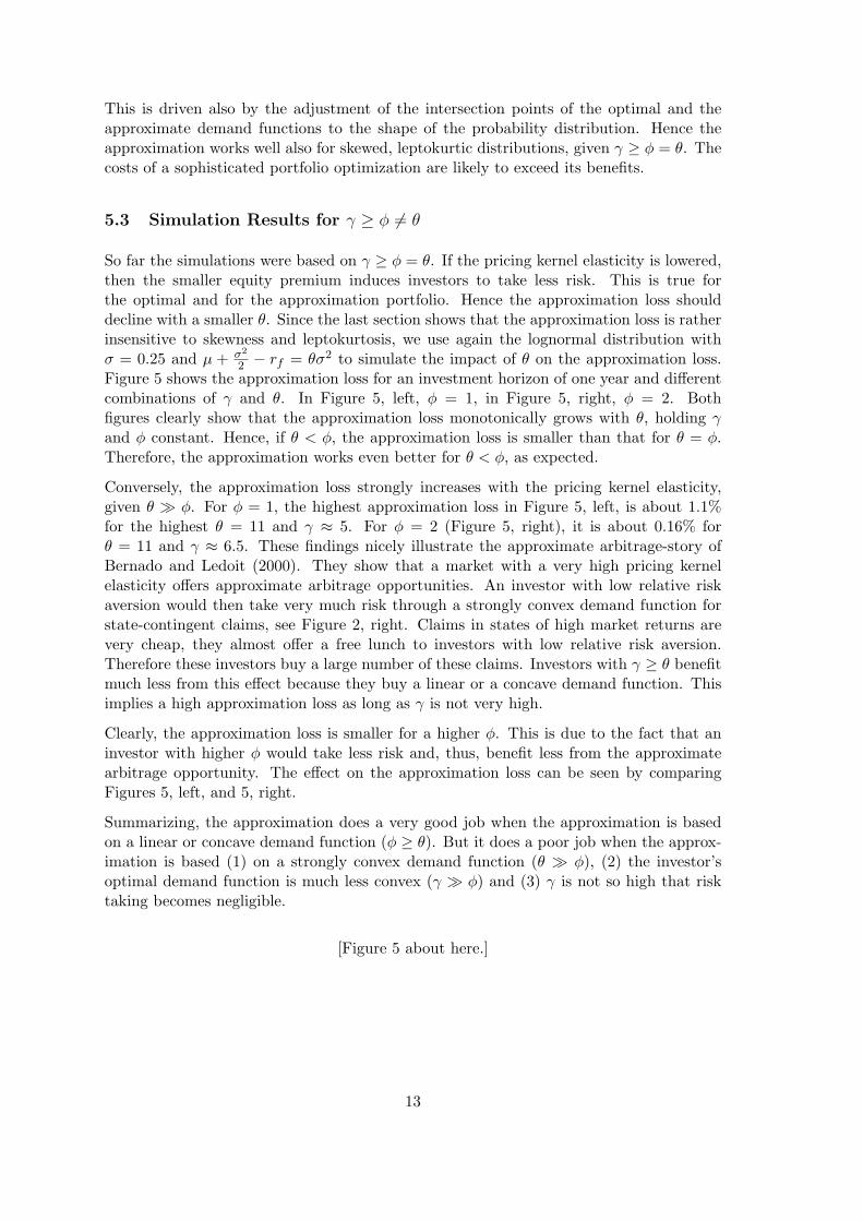
2 − rf = θσ2 to simulate the impact of θ on the approximation loss.Figure 5 shows the approximation loss for an investment horizon of one year and differentcombinations of γ and θ. In Figure 5, left, φ = 1, in Figure 5, right, φ = 2. Bothfigures clearly show that the approximation loss monotonically grows with θ, holding γand φ constant. Hence, if θ < φ, the approximation loss is smaller than that for θ = φ.Therefore, the approximation works even better for θ < φ, as expected.

Conversely, the approximation loss strongly increases with the pricing kernel elasticity,given θ � φ. For φ = 1, the highest approximation loss in Figure 5, left, is about 1.1%for the highest θ = 11 and γ ≈ 5. For φ = 2 (Figure 5, right), it is about 0.16% forθ = 11 and γ ≈ 6.5. These findings nicely illustrate the approximate arbitrage-story ofBernado and Ledoit (2000). They show that a market with a very high pricing kernelelasticity offers approximate arbitrage opportunities. An investor with low relative riskaversion would then take very much risk through a strongly convex demand function forstate-contingent claims, see Figure 2, right. Claims in states of high market returns arevery cheap, they almost offer a free lunch to investors with low relative risk aversion.Therefore these investors buy a large number of these claims. Investors with γ ≥ θ benefitmuch less from this effect because they buy a linear or a concave demand function. Thisimplies a high approximation loss as long as γ is not very high.

Clearly, the approximation loss is smaller for a higher φ. This is due to the fact that aninvestor with higher φ would take less risk and, thus, benefit less from the approximatearbitrage opportunity. The effect on the approximation loss can be seen by comparingFigures 5, left, and 5, right.

Summarizing, the approximation does a very good job when the approximation is basedon a linear or concave demand function (φ ≥ θ). But it does a poor job when the approx-imation is based (1) on a strongly convex demand function (θ � φ), (2) the investor’soptimal demand function is much less convex (γ � φ) and (3) γ is not so high that risktaking becomes negligible.


13

5.4 Non-Constant Elasticity of the Pricing Kernel

So far we assumed constant elasticity of the pricing kernel for the market return. Ait-Sahalia and Lo (2000), Jackwerth (2000), Rosenberg and Engle (2002), Bliss and Pani-girtzoglou (2004), Barone-Adesi, Engle and Mancini (2008) estimate the elasticity of thepricing kernel using prices of options on the S&P 500 and the FTSE 100. They concludethat the pricing kernel elasticity is declining, perhaps with a local maximum in between.

If the pricing kernel of the market portfolio does not have constant elasticity, we derivea transformed market portfolio such that its pricing kernel has low constant elasticity.Then, instead of the market portfolio, we use this transformed market portfolio for theapproximation. Assume that the elasticity ν(RM ) = −∂ lnπ(RM )/∂ lnRM is positive andnon-constant. Let RTM := g(RM ) := exp

{1θ

∫ RMε ν(R0

M )d lnR0M

}, where θ is a small,

positive constant. ε is a positive lower bound of RM . g is invertible and yields a pricingkernel π of constant elasticity θ with respect to RTM . This follows since

− lnπ(RM ) + lnπ(ε) =∫ RM

εν(R0

M )d lnR0M

= θ ln g(RM )= θ lnRTM= − ln π(RTM ) + lnπ(ε). (25)

The per unit-probability price for a claim contingent on RTM , π(RTM ), equals π(RM ),the price for a claim contingent on RM = g−1(RTM ). By definition, RTM is a one-to-onetransformation of the market return so that constant elasticity θ of the new pricing kernelπ(RTM ) is assured. This is true regardless of the sign of ν ′(RM ). Moreover, the levelof the constant pricing kernel elasticity of the transformed market return can be chosenfreely. Therefore, we can always create an exchange traded fund (ETF) on the marketreturn with return RTM and low constant elasticity θ of its pricing kernel. This ETF is asuitable candidate for the approximation portfolio so that

V −(RTM ) =θ

RfRTM + (γ − θ); γ ≥ θ.

This approximation assures a low approximation loss.

5.5 Incomplete Markets

So far we considered complete markets. In an incomplete market, the pricing kernel is nolonger unique. Suppose, first, that a pricing kernel on the market with low constant elas-ticity is feasible. For this case the preceding analysis has shown that buying the marketportfolio and the risk-free asset provides a very good approximation to the optimal port-folio for a large variety of settings. Actually, in an incomplete market the approximationquality is even better. This follows because incompleteness does not affect the availabilityof the market portfolio and, hence, the approximation portfolio, but the optimal portfolioin a complete market may not be available. This reduces the the approximation loss.

14

Second, suppose that a pricing kernel with low constant elasticity is not feasible. Then wecan use an ETF. If both, the ETF and the portfolio which would be optimal in a completemarket, cannot be replicated exactly in an incomplete market, then the approximation lossmight go up or down. But, given a large number of available risky assets, the differencebetween a complete and an incomplete market should be small.

5.6 Extension to Parameter Uncertainty

So far all parameters are assumed to be known precisely. The discussion on parameteruncertainty focusses on the probability with which one portfolio is preferable to anotherone in the presence of parameter uncertainty. As discussed before, several papers concludethat, given a set of well-diversified portfolio strategies, no strategy significantly outper-forms the other strategies. To address this issue, consider the following setting. Initiallythe investor buys a portfolio of state-contingent claims based on the a priori probabil-ity distribution of the market return. The pricing kernel is consistent with the a prioridistribution. In the spirit of the papers on parameter uncertainty, we derive the a prioriprobability that ex post, i.e. given the a posteriori distribution, the ex ante optimal port-folio is still preferred to the approximation portfolio. Let I denote the parameter vectorof the a posteriori distribution of the market return. Hence, we check

P = Prob[I∣∣∣ ce(V +|I) ≥ ce(V −|I)

], (26)

where ce(V |I) is the certainty equivalent of portfolio payoff V , given the a posterioridistribution I.

To illustrate, assume that each a posteriori distribution of the market return is log normal,n(lnRM |I). Then the a priori probability density of RM is given by

∫n(lnRM |I)dF (I),

with F (I) being the cumulative probability distribution of I. We use a symmetrictruncated normal distribution for I = [E[RM ], σ(RM )] with bounds [0.8955; 1.2955] forE[RM |I] and [0.1782; 0.3782] for σ(RM |I). We assume that E[RM |I] and σ(RM |I) areuncorrelated and that the standard deviation of both parameters is 0.1. This yields ana priori probability distribution of RM with simulated expected market return of 1.0974and standard deviation of 0.2942. This distribution is not log normal. Given the a prioridistribution, we derive exp{a(γ)} by simulation and obtain the optimal demand V +(RM ).The linear demand function V −(RM ) is based on φ = θ = 1 and is independent of thedistribution. Figure 6 plots the certainty equivalent difference, ce(V +|I)− ce(V −|I), fora time horizon of 1 year and for γ = 3, γ = 8 and γ = 50. Also, the plot illustrates theI-range for which this difference is positive, i.e. it is above the black zero hyper-plane. Thea priori probability of this range is P ≈ 0.75 for all γ-values. Hence, the optimal portfoliodoes not outperform the approximation portfolio at any conventional significance level.Therefore, the regret probability (1−P) of not having chosen the approximation portfoliois substantial.

This finding is not surprising because the approximation portfolio payoff is linear in themarket return while the optimal payoff is concave. The certainty equivalent of the linearpayoff is less sensitive to parameter variations than that of the concave payoff. Since, apriori, the certainty equivalent of the optimal portfolio exceeds that of the approximationportfolio only by a small percentage, we can only expect a high probability P if the a

15

posteriori certainty equivalent of the optimal portfolio is as stable as that of the approxi-mation portfolio with respect to parameter variations. But as illustrated in Figure 6, thisis not true. Therefore the investor faces a rather high regret probability (1−P). This maybe viewed as another argument for choosing the simple approximation portfolio instead ofthe complicated optimal portfolio.


6 Approximation in a Discrete State Space

In a continuous state space the probability mass of the optimal and the approximationportfolio payoff may be concentrated around the zero excess payoff inducing a strongapproximation quality. This quality might be weaker for portfolio returns with moreprobability mass in the tails. Lemma 1, however, suggests that the approximation loss issimilar in a continuous and a discrete state space whenever the non-central moments are.To find out about these effects, we now analyze the approximation quality in a discretestate space with few states.

As an example, consider a bank which only invests in loans. The loan market is arbitragefree. Loans either are fully paid or go into default paying a non-random recovery amount.If the bank can invest in many different loans, it can achieve strong portfolio diversification.Then the loan portfolio payoff can be approximated quite well by a continuous unimodalprobability distribution. This suggests again a high approximation quality in the absenceof approximate arbitrage opportunities. Critical might be cases in which the number ofloans is small. In the following, we present examples with one and two loans.

6.1 One Risky Asset

In the case of only one risky asset, there is no structure effect. Yet, the volume effect(α+ − α−) remains and determines the approximation loss. A volume effect would notexist if the 1/γ-rule would work perfectly. α+ = α(γ) and α− = α(φ) denote the optimaland the approximate amount invested in the single risky asset, derived from the first orderconditions (3) respectively (5).

We analyze a negatively and a positively skewed binomial distribution. Both distributionshave the same expected return of 10.5% and standard deviation of 30% so that the Sharpe-ratio is the same. The risk-free rate is 3%. Let u (d) be the gross return in the up-state (down-state). p is the up-state probability for the distribution R skewed to theright and also the down-state probability for the distribution L skewed to the left. Forexample, let p = 0.25, uR = 1.42 and dR = 1, uL = 1.21 and dL = 0.79. Hence thedistribution R has a skewness of 0.191, while distribution L has a skewness of −0.165.The approximated investment in the risky asset is the optimal investment using φ = 1.The optimal investment, the volume effect and the approximation loss are shown in Table1 for an investor with constant relative risk aversion γ = 2, γ = 3 and γ = 10.

[Table 1 about here.]

16

The volume effect is negative (positive) for the positively (negatively) skewed return dis-tribution. The volume effect relative to the optimal investment in the risky asset is ratherlarge (small) for the positively (negatively) skewed distribution. Yet, the approximationloss is rather small in all cases. It is larger for the positively skewed distribution, anddeclines with increasing γ for high values of γ.

The intuition for the sign of the volume effect can be derived from Figure 1. The optimalvolume depends on the absolute risk aversion levels in the down-state and the up-state.Given γ > φ, the absolute risk aversion is higher [smaller] for the utility function withparameter φ than for that with parameter γ in the down-state [up-state].

For the positively skewed distribution the absolute difference in risk aversion is muchhigher in the up-state than in the down-state. Therefore we expect a negative volumeeffect, α+ < α−. For a negatively skewed distribution we expect a positive volume effect.This is confirmed in Table 1. For a symmetric distribution, the absolute difference in riskaversion is about the same in the down- and in the up-state. Therefore α+(γ) ≈ α−(φ)implying a very small volume effect.

There is an easy way to understand the strong volume effect for the positively skeweddistribution. For a binomial distribution, the first order condition yields

puru

(1 +

α+ruγ

)−γ= (1− pu)|rd|

(1 +

α+rdγ

)−γ⇔ puru

(1− pu)|rd|=(γ + α+ruγ + α+rd

)γ. (27)

The left hand side of (27) denotes the gain/loss- ratio of Bernado and Ledoit (2000).The higher it is, the closer is an approximate arbitrage opportunity. For the positively(negatively) skewed distribution the gain/loss- ratio is 4.33 (2.25). Hence, the positivelyskewed distribution is much closer to approximate arbitrage. An investor with low relativerisk aversion benefits more from approximate arbitrage than an investor with higher riskaversion by choosing a more aggressive portfolio. This explains for φ = 1 the high value ofα− = 6.41, the strong negative volume effect and the relatively high approximation loss.

As argued by Bernado and Ledoit, a high elasticity of the pricing kernel indicates anapproximate arbitrage opportunity4. The pricing kernel elasticity is 4.18 (1.90) for thepositively (negatively) skewed distribution. Hence, the higher elasticity for the positivelyskewed distribution also motivates a higher approximation loss.

6.2 Two Risky Assets with Dependent Returns

Next, consider two risky loans with correlated binomial returns. In this case there existonly 4 states of nature. If there are two loans with different expected returns and perfectlynegatively correlated returns, then there exists an arbitrage opportunity. If the returnsare strongly negatively correlated, then there exists an approximate arbitrage opportunity.Hence, investors with low relative risk aversion will take very large positions in the riskyassets which should raise the approximation loss.

For illustration, let the marginal distribution of each risky asset have a binomial distribu-tion with equal probability for both outcomes, the up-state and the down-state. The gross

17

return of asset 1 is R1 = (1.2; 0.925) and of asset 2 is R2 = (1.3; 0.85), respectively. Therisk-free rate is 3%. This implies an expected excess return of 3.25% for asset 1 and 4.5%for asset 2. The standard deviation is 13.75% for the first asset and 22.5% for the secondasset. Holding the marginal distributions for both asset returns constant, we change thereturn correlation by the following procedure. Let Ps,t := Prob(R1 = s,R2 = t) denotethe probability that asset 1 is in the s-state and asset 2 is in the t-state, s, t ∈ {up, down}.Then, the joint probability is

[Ps,t]s,t∈{up, down} =(

0.5− x xx 0.5− x

),

with x ∈ [0; 0.5]. Reducing Pup, up and Pdown, down by x and adding x to Pdown, up andPup, down, decreases the correlation without affecting the marginal distributions.

The approximation portfolio is based on φ = 0.98. For relative risk aversion γ ∈ [0.98; 8]and for a return correlation between -0.8 and 0.8, Figure 7, left, shows the approximationloss. It is very low for correlations above -0.5, but increases strongly for lower correlations.Given negatively correlated assets, the investor can buy a hedged portfolio with longpositions in both assets and earn a high portfolio return with little downside potential.Consider the case with correlation −0.6 and γ = 2.5. The optimal portfolio invests about3.57$ of the initial endowment in asset 1 and about 2.06$ in asset 2. This gives anexpected excess return of the optimal portfolio of 8.61% and a standard deviation of17.64%. The approximation portfolio invests 3.02$ in asset 1 and 1.70$ in asset 2 implyingan approximation loss of about 0.15%. The volume effect is (3.57 + 2.06)− (3.02 + 1.70) =0.91$, it is quite strong. The structure effect 3.57

2.06 −3.021.70 = −0.04 is, however, very weak.

For higher correlations, the approximation quality is excellent.


Figure 8 shows the volume and the structure effect. The volume effect is quite strongfor strongly negative correlation, while the structure effect is always quite modest. Thisindicates that the approximation quality is impaired primarily by the volume effect.


The example shows that the approximation loss is substantial whenever the asset corre-lation supports an approximate arbitrage. Then the investor with low RRA φ takes largepositions in both risky assets and borrows a lot. If we exclude short selling, then approx-imate arbitrage opportunities cannot be used extensively so that the approximation lossis much smaller. This is illustrated in Figure 7, right. Compared to Figure 7, left, therestriction lowers the approximation loss strongly in the area [−0.8,−0.4]× [1.75, 4], wherethe first dimension is the asset correlation and the second the relative risk aversion γ.

7 Conclusion

Sophisticated portfolio optimization is unlikely to pay in a large variety of settings. Weconstrain our analysis to HARA-investors with declining absolute risk aversion and ask

18

whether the parameters of the utility function really matter for optimal investment deci-sions. The paper shows that the optimal portfolio can be approximated without noticeableharm by the portfolio which is optimal for some HARA-investor with lower relative riskaversion, if approximate arbitrage opportunities do not exist. If these opportunities existand the approximation portfolio takes high risk while the optimal portfolio does not, thenthe approximation leads to high approximation losses. Whenever the pricing kernel of themarket return displays constant elasticity, an investor with higher relative risk aversionmay simply buy the market portfolio and the risk-free asset without noticeable harm. Oth-erwise, the investor may buy a transformed market portfolio with low constant elasticityof the pricing kernel. Critical for a strong approximation quality is that the investor’srelative risk aversion is higher than that used for the approximation and that approximatearbitrage opportunities do not exist.

Our findings generalize the two fund-separation of Cass and Stiglitz such that differencesin the structures of optimal risky funds, driven by different levels of relative risk aversion,matter little in the absence of approximate arbitrage opportunities.

If there exists uncertainty about the parameters of the asset returns, then our examplesdemonstrate that the approximation portfolio turns out to be better than the optimalportfolio with a substantial probability. This also supports the use of a simple approx-imation portfolio. Further research might analyse the approximation quality in marketsettings in which investors use dynamic trading strategies to benefit from stock returnpredictability. Also the set of utility functions should be widened beyond HARA.

19

A Footnotes

1For small portfolio risk, mi → 0 for i > 2. Then the optimal portfolio satisfies m1/m2 → 1 renderingγ irrelevant. This is the case in a continuous time model with i.i.d. returns. Then the volume and thestructure effect disappear.

2The skewness is skt = 4−π2

“δt

√2/π

”3

(1−2δ2t /π)3/2 and the excess kurtosis is 2(π − 3)

“δt

√2/π

”4

(1−2δ2t /π)2.

3Independent increments imply skt = sk1/√t, where sk1 denotes the skewness for one year and skt is

the skewness for t-years.

4Consider the Arrow-Debreu prices in this complete market setting. For a binomial return there alwaysexists a pricing kernel with constant elasticity. The two Arrow-Debreu prices are

πu =1

Rf

puR−θu

E[R−θ]and πd =

1

Rf

(1− pu)R−θdE[R−θ]

.

The ratio πuπd

can be used to solve for the pricing kernel elasticity θ,

θ =

ln

gain-loss-ratio

!ln“RuRd

” .

20

B Proof of Lemma 3

At an intersection point, V +(RjM ) = V −(RjM ). Then, we have at an intersection withR = RjM ,

∂V +(R)∂p

=∂V −(R)∂p

⇔ θ

γexp{a(γ)}R(θ/γ)−1∂R

∂p+∂a(γ)∂p

V +(R) =θ

φexp{a(φ)}R(θ/φ−1)∂R

∂p+∂a(φ)∂p

[V −(R)−(γ−φ)

]Since V +(R) = V −(R), we have

θ

γV +(R)

∂ lnR∂p

+∂a(γ)∂p

V +(R) =[ θφ

∂ lnR∂p

+∂a(φ)∂p

][V +(R)− (γ − φ)]

⇔ ∂ lnR∂p

θ

φ

1γ

(γ − φ)[V +(R)− γ] =[∂a(γ)∂p

− ∂a(φ)∂p

]V +(R) +

∂a(φ)∂p

(γ − φ).

Dividing by (γ−φ) yields equation (20). Equations (21) and (22) follow from differentiatingthe budget constraint with respect to p.

21

References

[1] Ait-Sahalia, Y. and A. W. Lo, 2000, ”Nonparametric risk management and impliedrisk aversion”, Journal of Econometrics 94, 9-51.

[2] Arrow, K. J., 1974, ”Essays in the Theory of Risk-Bearing”, Markham Publishing Co.

[3] Balduzzi, P. and A. Lynch, 1999, ”Transaction Costs and Predictability: Some UtilityCost Calculations”, Journal of Financial Economics 52, 47-78.

[4] Barone-Adesi G., R. F. Engle and L. Mancini, 2008, ”A GARCH Option Pricing Modelwith Filtered Historical Simulation”, Review of Financial Studies 21, 1223-1258.

[5] Bernado, A. and O. Ledoit, 2000, ”Gain, Loss and Asset Pricing”, Journal of PoliticalEconomy 108, 144-172.

[6] Black, F., R. Littermann, 1992, ”Global Portfolio Optimization”, Financial AnalystsJournal, Sept/Oct. 28-43.

[7] Bliss, R. R. and N. Panigirtzoglou, 2004, ”Option-Implied Risk Aversion Estimates”,Journal of Finance 59, 407-446.

[8] Brandt, M., A. Goyal, P. Santa-Clara and J. Stroud, 2005, ”A Simulation Approach toDynamic Portfolio Choice with an Application to Learning About Return Predictabil-ity”, Review of Financial Studies 18, 831-873.

[9] Brandt, M., P. Santa-Clara and R. Valkanov, 2009, ”Parametric Portfolio Policies:Exploiting Characteristics in the Cross Section of Equity Returns”, Review of FinancialStudies 22, 3411-3447.

[10] Cass, D., and J. E. Stiglitz, 1970, ”The structure of investor preferences and assetreturns, and separability in portfolio allocation: A contribution to the pure theory ofmutual funds”, Journal of Economic Theory 2, 122-160.

[11] Chacko, G. and L. Viceira, 2005, ”Dynamic Consumption and Portfolio Choice withStochastic Volatility in Incomplete Markets”, Review of Financial Studies, 18, 1369-1402.

[12] Corrado, C. J. and T. Su, 1997 ”Implied Volatility Skews and Stock Index Skewnessand Kurtosis in S&P 500 Index Option Prices.”, Journal of Derivatives, 4, 8-19.

[13] DeMiguel, V., L. Garlappi and R. Uppal, 2009, ”Optimal versus Naive Diversification:How Inefficient is the 1/N Portfolio Strategy?”, Review of Financial Studies 22, 1915-1953.

[14] DeMiguel, V., L. Garlappi, J. Nogales and R. Uppal, 2009, ”A Generalized Approachto Portfolio Optimization: Improving Performance By Constraining Portfolio Norms”,Management Science 55, 798-812.

[15] Diamond, P. A. and J. E. Stiglitz, 1974, ”Increase in Risk and Risk Aversion”, Journalof Economic Theory 66, 522-535.

[16] Hakansson, N. H. 1970, ”Optimal Investment and Consumption Strategies UnderRisk for a Class of Utility Functions”, Econometrica, 38, 587-607.

22

[17] Hodder, J., J. Jackwerth and O. Kokolova, 2009, ”Improved Portfolio Choice UsingSecond Order Stochastic Dominance”, Working paper, University Konstanz.

[18] Jackwerth, J., 2000, ”Recovering Risk Aversion from Option Prices and RealizedReturns”, Review of Financial Studies 13, 433-451.

[19] Jacobs, H., S. Mueller and M. Weber, 2009, ”How Should Private Investors Diversify?An Empirical Evaluation of Alternative Asset Allocation Policies to Construct a ’WorldMarket Portfolio”, Working paper, University of Mannheim.

[20] Karatzas, I., J. Lehoczky, S. Sethi, S. Shreve, 1986, ”Explicit Solution of a GeneralConsumption/Investment Problem”, Mathematics of Operations Research 11, 261-294.

[21] Merton, R. C. 1971, ”Optimal Consumption and Investment Rules in a ContinuousTime Model”, Journal of Economic Theory 3, 373-413.

[22] Pratt, J. W., 1964, ”Risk Aversion in the Small and in the Large”, Econometrica 32,122-136.

[23] Rosenberg, J. V. and R. F. Engle, 2002, ”Option Hedging Using Empirical PricingKernels”, Journal of Financial Economics 64, 341-372.

[24] Rothschild, M. and J. E. Stiglitz, 1970, ”Increasing Risk I: A Definition”, Journal ofEconomic Theory 2, 225-243.

[25] Viceira, L. (2001), ”Optimal Portfolio Choice for Lang-Horizon Investors with Non-tradable Labor Income”, Journal of Finance 61,433-470.

23

−0.5 0 0.50.8

0.9

1

1.1

1.2

1.3

1.4

1.5

Excess Return

Abs

olut

e R

isk

Ave

rsio

n

gamma = 2gamma = 3gamma = 4gamma = 5gamma = 15

Figure 1: The absolute risk aversion of the HARA-function with endowment γ/Rf declines in theportfolio excess return. For increasing γ the difference between the absolute risk aversion of theHARA-function and that of the exponential utility function, being 1 everywhere, decreases.

24

Figure 2: Left: The figure shows the optimal demand for state contingent claims (blue solidcurve) and the approximation demand (red dotted line) for γ = 3 ≥ φ = θ = 1.25. In addition,on a different scale the graph shows the probability density of the market return. Right: γ = 3,θ = 6.75 and φ = 1. This implies a strongly convex approximation demand function while theoptimal demand function is only moderately convex.

25

Figure 3: Left: The surface shows the approximation loss for γ ∈ [0.98; 8], φ = θ = 0.98 and aninvestment horizon between 3 months and 5 years. For this setting, the highest loss in certaintyequivalent is obtained for γ between 3 and 4 and an investment of five years. The investor wouldhave lost about 0.3% of the optimal certainty equivalent or 0.06% per year. Right: Each isoquantshows the combination of γ and investment horizon with the same approximation loss k depictedin the curve.

26

Figure 4: The surface shows the approximation loss for γ ∈ [0.98; 8], φ = θ = 0.98 and aninvestment horizon between 3 months and 5 years. Left: The logarithmic market return is t-distributed. We assume independent and identically distributed increments, hence, µt = 0.06t, σt =0.25√t and νt = 4t+4. For γ ≈ 3 and an investment horizon of five years, the highest approximation

loss is about 0.4%. Right: The logarithmic market return is left-skewed, fat tailed distributedwith independent and identically distributed increments.

27

Figure 5: Left: The approximation loss for an investment horizon of one year as a function ofθ and γ, assuming a lognormal market return with σ = 0.25. rf = 0.03 and φ = 1. γ ∈ [φ; 20] ,θ ∈ [0.44; 11]. Right: The approximation loss for the same setting as in Figure 5, left, but withφ = 2.

28

Figure 6: The plot shows the a posteriori-approximation loss assuming parameter uncertainty.The expected market return and the market volatility are a posteriori-realisations of both variables.The blue (red) [green] surface shows the loss assuming γ = 3 (γ = 8) [γ = 50], the black hyper-planemarks zero everywhere.

29

Figure 7: γ > φ = 0.98, correlation of binomial returns between -0.8 and 0.8. Left: The figuresshow the approximation loss in a market with two binomial assets for different return correlationsand γs. The expected excess return for asset 1 is 3.25% and 4.5% for asset 2. The volatility is13.75% and 22.5%, respectively. Right: The figure shows the approximation loss for the samemarket setting with borrowing being prohibited.

30

Figure 8: Left: The volume effect for a market with two binomial assets as in Figure 7. Onlyfor strongly negative asset correlation there is a substantial volume effect. Right: The structureeffect is remarkably small.

31

γ = 2 γ = 3 γ = 10Distribution R L R L R L

α+ 4.7813 1.8519 4.3083 1.8830 3.7183 1.9187(α+ − α−) −1.6290 0.1158 −2.1020 0.1469 −2.6920 0.1826

k 0.0038 0.0002 0.0048 0.0002 0.0028 0.0001

Table 1: It shows the optimal investment in the risky asset for γ = 2, 3 and 10 and the volumeeffect (α+ − α−). The approximated investment based on φ = 1 is α− = 6.4103 for R andα− = 1.9677 for L. k is the approximation loss. R (L) denotes the probability distribution skewedto the right (left)

32

does portfolio optimization pay?

Documents