Does OTC Derivatives Reform Incentivize Central Clearing?

16-07 | July 26, 2016

Samim Ghamami Office of Financial Research samim.ghamami@ofr.treasury.gov

Paul GlassermanOffice of Financial Research and Columbia University paul.glasserman@ofr.treasury.gov

The Office of Financial Research (OFR) Working Paper Series allows members of the OFR staff and their coauthors to disseminate preliminary research findings in a format intended to generate discussion and critical comments. Papers in the OFR Working Paper Series are works in progress and subject to revision.

Views and opinions expressed are those of the authors and do not necessarily represent official positions or policy of the OFR or Treasury. Comments and suggestions for improvements are welcome and should be directed to the authors. OFR working papers may be quoted without additional permission.

Does OTC Derivatives Reform Incentivize Central Clearing?∗

Samim Ghamami† and Paul Glasserman‡

Abstract

The reform program for the over-the-counter (OTC) derivatives market launched by the G-20 nationsin 2009 seeks to reduce systemic risk from OTC derivatives. The reforms require that standardized OTCderivatives be cleared through central counterparties (CCPs), and they set higher capital and marginrequirements for non-centrally cleared derivatives. Our objective is to gauge whether the higher capi-tal and margin requirements adopted for bilateral contracts create a cost incentive in favor of centralclearing, as intended. We introduce a model of OTC clearing to compare the total capital and collateralcosts when banks transact fully bilaterally versus the capital and collateral costs when banks clear fullythrough CCPs. Our model and its calibration scheme are designed to use data collected by the FederalReserve System on OTC derivatives at large bank holding companies. We find that the main factorsdriving the cost comparison are (i) the netting benefits achieved through bilateral and central clearing;(ii) the margin period of risk used to set initial margin and capital requirements; and (iii) the levelof CCP guarantee fund requirements. Our results show that the cost comparison does not necessarilyfavor central clearing and, when it does, the incentive may be driven by questionable differences inCCPs’ default waterfall resources. We also discuss the broader implications of these tradeoffs for OTCderivatives reform.

JEL Codes: G01, G18, G20, G28.

Keywords: Central clearing, OTC derivatives, margin, collateral, capital.

1 Introduction

In response to the financial crisis of 2008, leaders of the Group of Twenty nations agreed to reforms in

the over-the-counter (OTC) derivatives markets with the goal of reducing the systemic risk posed by these

∗We thank the Division of Banking Supervision and Regulation at the Federal Reserve Board and the Supervision Divisionof the Federal Reserve Bank of New York for graciously providing the confidential supervisory data used in this study. Weare grateful to Michael Gibson and Sean Campbell for helpful discussions on an earlier version of our work. We thank LaxmiGrabowski for providing comments on the dataset and Erica Lee, Ning Luo, and Kapo Yuen for providing comments on theBIS International Data Hub initiative. We have benefited from helpful discussion with Charles Calomiris, Michael Gordy,David Murphy, and comments provided by the 2016 seminar participants at the Federal Reserve Bank of New York, FederalReserve Board, the NYU Salomon Center, Bank of England, Imperial College Mathematical Finance Group, Office of FinancialResearch, the Bank for International Settlements, the International Monetary Fund, and the U.S. Commodity Futures TradingCommission. The opinions expressed in this paper are those of the authors and do not necessarily reflect the views of theBoard of Governors, the Office of Financial Research, or their staff.†Office of Financial Research, email: samim.ghamami@ofr.treasury.gov, and University of California, Berkeley, Center for

Risk Management Research, email: samim ghamami@berkeley.edu.‡Office of Financial Research, email: paul.glasserman@ofr.treasury.gov, and Columbia Business School. This paper was

produced while Paul Glasserman was under contract with the Office of Financial Research and not an employee. He alsoserves as an independent member of the risk committee of a swaps clearinghouse.

1

markets. This program of reforms, launched in 2009, includes the following two elements:1

• All standardized OTC derivatives should be cleared through central counterparties (CCPs);

• Non-centrally cleared derivatives contracts should be subject to higher capital and collateral require-

ments.

An important motivation for the second of these elements is to create a cost incentive in favor of central

clearing (BCBS and IOSCO [2015]). Our goal is to evaluate whether this objective has been met and to

identify the main drivers of the cost comparison and their implications.

In a centrally cleared market, after two parties agree to an OTC derivative transaction, they replace

their bilateral contract with two back-to-back contracts through a CCP. The original bilateral relationship

is eliminated, and each of the two original parties continues to face the CCP throughout the life of the

contract. In a market without central clearing, the two original parties would instead face each other.

A centrally cleared market offers potential netting and operational benefits; it may be better able to

respond to the failure of a market participant; and it may yield greater transparency. It may also create a

network of exposures that is more vulnerable to a single point of failure (see the remarks by Bernanke [2011]

and Yellen [2013] on various aspects of CCPs and their role in financial stability and financial reform). The

effect of derivatives CCPs on financial stability, and the right design and regulation of the OTC derivative

market continue to generate debate among industry participants, government officials, and the public;

research and discussion of these questions includes Culp [2010], Stulz [2010], Singh [2010], Duffie and Zhu

[2011], Heller and Vause [2012], Pirrong [2011], Pirrong [2013], Cont and Kokholm [2014], Duffie et al.

[2015], Duffie [2016], and France and Kahn [2015].

The goal of this paper is to gauge whether new rules imposed on bilateral trading2 achieve the objective

of incentivizing central clearing, and to identify the main factors driving the cost comparison and their

implications. The cost comparison requires some assessment of both types of markets, particularly the

associated netting efficiency and risk management practices. Creating a cost incentive for central clearing

is a specific objective of the OTC derivatives reform program (see BIS [2014] and BCBS and IOSCO

[2015]). It remains relevant, despite the clearing mandate, because the question of when a contract is

sufficiently standard to require central clearing involves some discretion. Single-name credit default swaps,

for example, continue to trade both bilaterally and through CCPs. In the absence of a cost advantage

for central clearing, market participants may be motivated to customize contracts in order to trade them

bilaterally. Without a cost advantage, banks may also be less inclined to move legacy trades to CCPs.

1See Bernanke [2011], Yellen [2013], Fischer [2015], BCBS and IOSCO [2015], and the references therein for additionalbackground.

2We use the term “bilateral trading” as a simple way to refer to the part of the market that is not centrally cleared.The term is imprecise because even centrally cleared OTC contracts are initially traded bilaterally, rather than through anexchange, and then novated to a CCP. The more precise but more cumbersome term is “non-centrally cleared derivatives.”

2

We limit our analysis to the capital and collateral costs of bilateral trading and central clearing. We

take the perspective of a derivatives dealer within a bank holding company that is a clearing member of

the CCPs through which it trades. Under both bilateral trading and central clearing, the dealer faces

collateral costs resulting from margin requirements and capital charges resulting from counterparty credit

risk. Central clearing also requires contributions to a CCP’s guarantee fund,3 which carries both a collateral

and capital cost.

We compare these costs under two market configurations — a fully bilateral market and a fully centrally

cleared market. The detailed rules covering all the relevant costs are complex; we develop a simplified

framework that captures the key features driving these costs. Our model and its calibration are designed to

take advantage of a confidential dataset collected by the Federal Reserve Bank of New York and the Division

of Banking Supervision and Regulation at the Board of Governors of the Federal Reserve System. The

dataset provides information on institution-to-institution derivatives exposures, including some information

on both bilateral and centrally cleared transactions.

We find that three factors drive the comparison of costs between fully bilateral and fully centrally

cleared market configurations:

(i) the degree of netting achieved in each case;

(ii) the margin period of risk (MPOR) used to set initial margin and capital requirements in each case;

and

(iii) CCP risk management practices — specifically, their relative reliance on initial margin and guarantee

fund contributions.

Greater netting efficiency is often viewed as a benefit of central clearing through which total counter-

party risk in the financial system is reduced.4 In our cost comparison, greater netting lowers margin and

capital requirements. A single, global CCP clearing all derivatives would theoretically achieve maximal

netting efficiency. However, as noted by Duffie and Zhu [2011], Heller and Vause [2012], and Cont and

Kokholm [2014], central clearing may lose its netting advantage in a market with multiple CCPs. In our

analysis, the cost comparison is driven by the relative benefits of netting by counterparty versus netting

by product category. Although the importance of this tradeoff has been understood for some time, this

study is the first to be able to estimate these effects across multiple product categories using necessary

confidential data.5

3We use the terms “guarantee fund” and “default fund” interchangeably.4Pirrong [2013] argues that netting does not reduce risk but merely redistributes it by giving seniority to derivatives claims

over other claims. Whether netting is welfare-improving is an important question for the regulation of derivatives but it doesnot affect the cost comparison on which we focus.

5Duffie et al. [2015] compare bilateral and centrally cleared netting as well, but their analysis is limited to the CDS market.

3

Initial margin is intended to cover losses between the time of a counterparty’s default and the time the

position is closed out, known as the margin period of risk. This interval is currently set at five days for

centrally cleared OTC derivatives and ten days for bilateral trading. With all else equal, this difference

favors central clearing.

CCPs generally require clearing members to contribute to a guarantee fund through which losses to the

clearinghouse from the failure of one member are mutualized among surviving members. Guarantee fund

contributions create capital and collateral costs for member banks and thus favor bilateral trading. At the

same time, lowering these costs through smaller guarantee funds would undermine the financial stability

objective of the clearing mandate. We find wide variation in the practices of CCPs in setting their margin

and guarantee fund levels, which highlights the importance of this issue.

After taking into account these and other sometimes conflicting considerations and calibrating our

model to the Federal Reserve data, we cannot conclude that OTC derivatives reform creates an unam-

biguous cost incentive in favor of central clearing; indeed, for a wide range of realistic parameter values,

bilateral trading carries lower capital and collateral costs. This conclusion contrasts with a report from the

Bank for International Settlements (BIS [2014]), which finds that capital and collateral costs favor central

clearing. In addition to providing our overall comparison, our analysis allows a decomposition into the

key factors driving the tradeoff and their sensitivity to modeling assumptions, insights that are difficult to

glean from the results reported in BIS [2014]. Appendix C gives a brief discussion of BIS [2014].6

The rest of this paper is organized as follows. Section 2 reviews the pros and cons of central clearing

and the objectives of OTC derivatives reform that provide the backdrop to our investigation. Section 3

describes the capital and collateral rules we seek to capture in our analysis. Section 4 develops our model.

Section 5 describes our dataset and connects the data with the elements of our model. Section 6 discusses

the calibration of the model, and Section 7 presents our numerical results. In Section 8, we discuss the

main implications of our investigation.

2 OTC Derivatives Reform

To put our analysis in context, we briefly review the objectives of the clearing mandate for OTC derivatives

and the accompanying requirements of higher margin and capital requirements in the bilateral market.

OTC derivatives reform faces some competing objectives, and these tensions influence the cost comparison

we analyze.

As discussed in a joint report by the Basel Committee on Banking Supervision and the International

Organization of Securities Commissions (BCBS and IOSCO [2015]), margin requirements for non-centrally

6An article titled “Unclear incentives: do capital and margin rules support CCPs?” in Risk Magazine in March 20, 2015,also discusses various aspects of BIS [2014].

4

cleared derivatives serve two objectives: to reduce counterparty credit risk in the bilateral market, and to

promote central clearing. More broadly, central clearing of derivatives can support financial stability in

several ways:

• Requiring collateral for derivatives reduces counterparty credit risk.

• Central clearing can create greater opportunities for netting of derivatives, and netting also reduces

counterparty credit risk.

• Through its default management procedures, a CCP should be better prepared than the bilateral

market to deal with the failure of a major derivatives participant, managing an orderly disposal

of the failed party’s positions and the protection of its client’s trades. A CCP also monitors the

creditworthiness of its members and the risks they take on.

• Central clearing can improve price discovery and transparency. A CCP can observe the prices of

transactions among its members, and it can rely on its members to provide price quotes for marking

positions. This information might make a centrally cleared market less likely to freeze in times of

market stress.

• Through its default waterfall resources (margin and default fund contributions), a CCP absorbs losses

that would otherwise be borne by the derivatives counterparties of its member firms. This backstop

should reduce the risk of a downward spiral of collateral calls as a firm’s credit quality declines, as

happened in the case of American International Group, Inc., in 2008.

• Central clearing should facilitate regulatory oversight of the OTC derivatives market by allowing

regulators to monitor the market through CCPs rather than through a diffuse network of bilateral

transactions.

Critics of the clearing mandate for OTC derivatives argue that CCPs can threaten financial stability

by concentrating risk in institutions that might ultimately require government support in a crisis. The

extent to which the potential benefits of clearing listed above are realized in practice is also open to debate.

Moreover, many of these benefits are best achieved with fewer CCPs, so the advantages of central clearing

can be at odds with concerns over concentrating risk.

For our analysis, this tension between risk concentration and the advantages of central clearing is par-

ticularly relevant to the comparison of netting benefits with and without central clearing. The greatest

possible netting efficiency would be achieved by clearing all trades through a single CCP. Netting opportu-

nities are lost as market participants split their portfolios across multiple CCPs. In OTC clearing, CCPs

have generally limited the scope of products they clear, requiring separate clearing of interest rate swaps

5

and credit default swaps, for example; this separation limits spillovers from one market to another, but

it also reduces netting opportunities. We will see that the possibility of netting across product categories

also has a big impact on the bilateral market. Supervisory guidelines (BCBS and IOSCO [2015]) oppose

bilateral netting across product categories; this stance is conservative in the sense that it leads to higher

margin requirements, but it raises the question of whether collateral is a more effective tool for reducing

counterparty credit risk than netting.7

Several of the other benefits listed above for central clearing are also supported by having a smaller

number of CCPs. A CCP should be better able to monitor its members if it sees a greater fraction of its

members’ trades. The CCP should also be better able to sell the positions of a member in default if it does

not need to contend with other CCPs managing the same default at the same time, a point emphasized in

Glasserman et al. [2015].

Fragmentation of the OTC derivatives market has also been blamed for recent persistent price disloca-

tions. Standard U.S. dollar interest rate swaps have traded at different rates for the past year at the two

largest CCPs in this market. The difference is reportedly driven by a preference for one CCP over the other

among fixed-rate payers, because one CCP offers portfolio margining between swaps and listed Treasury

futures while the other does not. The trade imbalance creates a price difference that reflects the value

of greater netting opportunities. More recently, a price difference has emerged between yen denominated

interest rate swaps cleared in Japan and London, based in part on regulatory constraints on Japanese

banks. See Younger et al. [2016b] for a discussion of both of these examples of imbalances across CCPs.

We noted above that a CCP’s default waterfall resources generally, and default fund in particular, play

an important role in enhancing financial stability through central clearing. The capital and collateral costs

associated with default fund contributions will be an important part of our analysis — all else equal, they

raise the cost of central clearing. To the extent that regulators seek to promote central clearing over the

bilateral market, this raises the concern that default fund requirements might be relaxed.

As we discuss in Section 4, for CCPs designated systemically important, default waterfall resources are

required to meet a “Cover 2” standard, meaning that they should be sufficient to cover losses resulting

from the failure of any two clearing members under stress conditions. This is a principles-based standard

that leaves room for interpretation and implementation. Moreover, we will argue that the adequacy of the

Cover 2 standard, even if properly implemented, depends on the distribution of exposures across a CCP’s

members. We will quantify this effect through a parameter we call the concentration ratio. This parameter

will be important in our cost comparison.

7Some studies have raised concerns about the supply of high quality liquid assets required to meet the collateral demands ofOTC derivatives reform. See Anderson and Joever [2014], Heller and Vause [2012], and Sidanius and Zikes [2012] for analysisof this question.

6

3 Capital and Collateral Rules

Before proceeding to the details of our model, we describe the capital and collateral costs that banks

face when trading in the bilateral OTC markets and when trading through derivatives CCPs. The key

elements are summarized in Table 1 and illustrated in Box 1. Our model in Section 4 addresses each of

these elements.

Table 1: Banks’ collateral and capital requirements under bilateral and central clearing.Trading Bilaterally Clearing through CCPs

Collateral Requirements Initial MarginInitial Margin

Default Fund Contribution

Capital Requirements Counterparty Risk Capital CCP Risk Capital

3.1 Counterparty Risk Capital and CCP Risk Capital

Bilateral case. Suppose banks A and B are parties to a swap or other OTC derivatives contract. Suppose

the contract has positive value to bank A and therefore negative value to bank B. Then bank A is exposed

to the risk of default of bank B, and this exposure carries a capital requirement for bank A.

Under Basel III (BCBS [2011]), the capital charge for counterparty credit risk (CCR) has two elements.

The first is the Basel II CCR capital requirement, which is similar to the capital requirement bank A would

face if it had made a loan to bank B. In addition, Basel III includes a credit valuation adjustment (CVA)

capital requirement, which is intended to capture losses in the market value of bank A’s position with bank

B resulting from a decline in bank B’s creditworthiness without an outright default.8

Whereas the Basel II CCR capital requirement is a static calculation, CVA ordinarily reflects the

possibility that a counterparty may default at any time during an extended horizon and that the value

of the exposure may change over time (see Gregory [2012], Ghamami and Goldberg [2014], Carr and

Ghamami [2015], Pykhtin [2011] and the reference therein). Our model approximates a bank’s CCR risk

capital by multiplying Basel II pre-specified risk weight representing the counterparty’s credit quality

(default probability) by an average measure of the bank’s exposure to the counterparty.

The bank’s exposure must be calculated net of any collateral posted by the counterparty. We emphasize

this point because once banks exchange margin for bilateral transactions, the residual exposure — and the

resulting CCR capital requirement — should be small, even though a bank counterparty usually carries a

much higher risk weight than a CCP. 9

8See Goodhart [2011] for a comprehensive and insightful historical account of the BCBS, Hull [2012] for a description ofvariations of the Basel credit risk and counterparty risk capital rules.

9The static element of Basel III CCR capital requirement is calculated net of the CVA risk capital charge (pages 36-37 ofBCBS [2011]). The exposure at default (EAD) component of the CVA charge is reduced by potential “CVA hedges” using

7

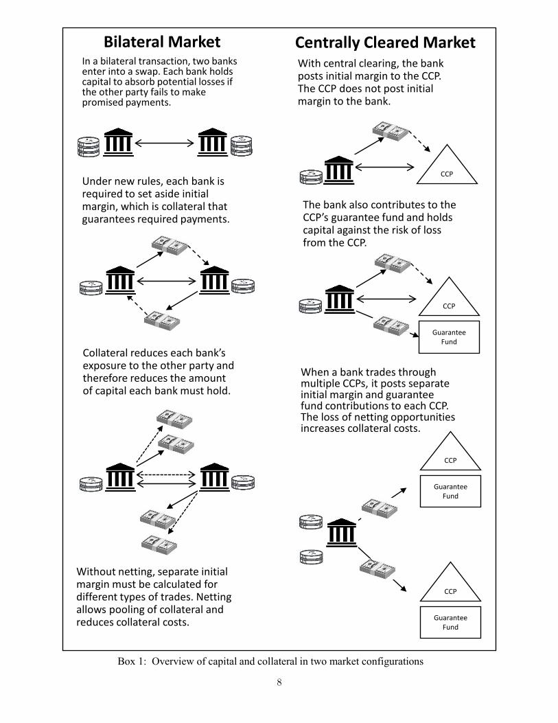
In a bilateral transaction, two banks enter into a swap. Each bank holds capital to absorb potential losses if the other party fails to make promised payments.

Under new rules, each bank is required to set aside initial margin, which is collateral that guarantees required payments.

Collateral reduces each bank’s exposure to the other party and therefore reduces the amount of capital each bank must hold.

Without netting, separate initial margin must be calculated for different types of trades. Netting allows pooling of collateral and reduces collateral costs.

CCP

With central clearing, the bank posts initial margin to the CCP. The CCP does not post initial margin to the bank.

CCP

The bank also contributes to the CCP’s guarantee fund and holds capital against the risk of loss from the CCP.

Guarantee Fund

CCP

Guarantee Fund

CCP

Guarantee Fund

When a bank trades through multiple CCPs, it posts separate initial margin and guarantee fund contributions to each CCP. The loss of netting opportunities increases collateral costs.

Bilateral Market Centrally Cleared Market

Box 1: Overview of capital and collateral in two market configurations

8

Centrally cleared case. When a bank trades through a CCP, it takes on counterparty risk through the

possibility that the CCP or its members may fail. This exposure carries a capital requirement.

Under Basel II and Basel III, the CCP risk capital requirement has two components. The bank incurs

a trade exposure capital charge, based on its exposure to the CCP in its current trades. This component

is similar to the Basel II capital charge a bank would face in trading with another bank, though typically

with a much lower risk weight for a CCP than for a bank. In addition, the bank incurs a default fund

exposure capital charge. This component is based on the risk that the bank’s contribution to the CCP’s

default fund would be tapped in the event of the failure of other clearing members.10 Our model of OTC

clearing closely follows the Basel II-III formulation to approximate banks’ CCP risk capital.

3.2 Collateral Requirements

Next, we describe collateral requirements in OTC derivatives trading. We first discuss requirements under

central clearing, then turn to the bilateral case.

Centrally cleared case. A CCP collects three types of collateral from its clearing members to protect

the CCP against the failure of a clearing member:

◦ variation margin (VM);

◦ initial margin (IM);

◦ prefunded contributions to the guarantee fund.

Variation margin reflects the daily (or intraday) marking-to-market of a clearing member’s portfolio with

the CCP. Depending on the direction of the market, VM is posted by the clearing member to the CCP or

credited to the clearing member’s account by the CCP.11 Whereas VM is based on realized price changes,

IM is based on potential price changes to which the CCP would be exposed following the default of a

clearing member. For example, IM is often set based on a value-at-risk (VaR) model measuring the 99th

percentile of the loss distribution (from the perspective of the CCP) over a risk-measurement horizon of

five days, which is the margin period of risk.

If a clearing member defaults, the CCP needs to replace the failed member’s positions to return the CCP

to a “matched book” with no net market risk. The margin period of risk is intended to be a conservative

credit default swap trades; it should also be reduced by margin requirements as mentioned above. Some computational aspectsof the CVA capital charge have not been finalized yet (pages 4-5 of BCBS [2016]). Our approximation of the CCR capitalcharge does not take in to account CCR hedges but captures margin requirements.

10See Ghamami [2015] for a detailed description of CCP risk capital charges.11We do not include VM payments in Table 1 because they reflect price settlements and, as we argue later, should be roughly

equal under bilateral and central clearing.

9

estimate of the time needed for this replacement. During this period the market may move, leading to losses

to the CCP. The CCP’s default waterfall is intended to allow the CCP to withstand these losses.12 The

CCP first taps the failed member’s VM and IM, and then the failed member’s contribution to the CCP’s

guarantee fund. If losses exceed the failed member’s contributions, the next layer of the default waterfall

is usually a layer of capital contributed by the CCP.13 Losses beyond that level are then absorbed by the

guarantee fund contributions of the surviving members. If the prefunded guarantee fund is depleted, the

CCP typically has the right to call for additional contributions from the surviving members. Our model

approximates the collateral cost to a clearing member of margin requirements and prefunded contributions

to the guarantee fund. We do not explicitly account for the potential costs of additional assessments,

except in the default fund exposure component of the CCP risk capital charge. Adding the funding costs

of assessments would increase the total cost of central clearing.

Bilateral case. Prior to the introduction of the 2009 reforms, the OTC derivatives market was not subject

to regulations requiring the exchange of margin between counterparties. The market developed its own

practices and legal arrangements regarding the exchange of variation margin (often at a weekly frequency)

and an independent amount at trade inception similar to initial margin. (See, e.g., Pykhtin and Zhu [2006]

for details of these practices.)

In the G-20 OTC derivatives reform program (BCBS and IOSCO [2012] and BCBS and IOSCO [2015]),

regulators have introduced VM and IM requirements in the non-centrally clearing OTC markets in a way

that closely resembles the VM and IM requirements at CCPs. VM is to be exchanged on a daily basis,

and IM is to be based on a margin period of risk of 10 days. In fact, BCBS and IOSCO [2015] states

that promotion of central clearing has been one of the motivations and perceived benefits behind bilateral

margin requirements.14 Our model captures the cost of collateral resulting from margin requirements in

the bilateral OTC markets.

In the overall cost comparison summarized in Table 1, two points are worth highlighting. First, although

IM collateral costs are included in both market configurations, the associated costs could be quite different,

even if the margining rules in the two scenarios were identical, because the portfolios in the two scenarios

would be different: in the bilateral case, portfolios are defined by counterparty; in the centrally cleared

case, we will form portfolios by product class because different classes of derivatives are generally cleared

12For more on CCP default waterfalls, see Duffie et al. [2010], Pirrong [2011], Cont [2015], Ghamami [2015] and referencestherein.

13This layer is often called the CCP’s skin in the game; it creates an incentive for the CCP to monitor and manage riskdiligently.

14Page 3 of BCBS and IOSCO [2015] states: “...(central) clearing imposes costs, in part because CCPs require margin tobe posted. Margin requirements on non-centrally cleared derivatives, by reflecting the generally higher risk associated withthese derivatives, will promote central clearing....”

10

through different CCPs.15 In contrast, the VM collateral costs should be approximately the same under

bilateral trading and central clearing, as long as all trades are subject to variation margin, because VM

reflects realized market moves and is therefore not dependent on how trades are grouped into portfolios.

The second point to emphasize about the costs in Table 1 is that capital and collateral costs will to some

extent offset each other, in the following sense: greater use of margin reduces exposure to a counterparty

and thus reduces the capital charge associated with the exposure. This is particularly important in the

bilateral case, where the counterparty risk weight is generally much larger. Thus, the added bilateral

collateral cost of the derivatives reform program is partly offset by a lower CCR capital charge, thereby

reducing the cost incentive for central clearing.

4 A Model of OTC Clearing Capital and Collateral Costs

In this section, we develop a model of the costs described in the previous section. We begin with a high-level

summary, then detail the analysis of costs in the bilateral and centrally cleared scenarios.

4.1 An Overview of the Model

We suppose there are K asset classes and N market participants simply referred to as banks. Each asset

class is cleared through a single CCP, which clears only that asset class. The asset class categories we

have in mind are interest rate swaps, credit default swaps, equity derivatives, commodity derivatives, and

foreign exchange derivatives. Consistent with our model, these categories of derivatives are typically cleared

through separate clearinghouses. Our assumption of a single CCP for each category is conservative in the

sense that trading through multiple CCPs reduces opportunities for netting and therefore increases costs.

We relax this assumption later.

Viewed from the perspective of bank i, central clearing is less costly than bilateral trading if

cl∑k

(IMik + DFik) + cp∑k

CCP-RCik < cl∑j=i

IMij + cp∑j=i

CCRij ,6 6

(1)

where the sums on the left run over asset classes k, and the sums on the right run over counterparties j.

For each asset class k, IMik and DFik are bank i’s initial margin and default fund contribution at CCP

k, and CCP-RCik is the capital charge incurred by bank i through its exposure to CCP k, assuming all

trades are centrally cleared. Similarly, under fully bilateral trading, IMij is the initial margin bank i posts

to bank j, and CCRij is the capital charge bank i incurs through its exposure to bank j. The coefficients

15Younger et al. [2016a] have recently studied initial margin cost incentives to clear swaptions with CME in the U.S. interestrate derivatives interdealer market. Considering a representative portfolio of trades, the paper concludes that dealers may notbe incentivized to clear. This is despite of the fact that at the single contract level, the bilateral IM model considered in theirstudy tends to produce higher margin than the central clearing IM model.

11

cl and cp measure the marginal cost of collateral and the marginal cost of capital for the bank. For these

coefficients, we will use the same values as in BIS [2013b] and BIS [2014], taking cl = 0.7 percent and

cp = 6.7 percent.

Each term in each of the sums in (1) depends on the risk in a portfolio. Each term on the left depends

on the risk of bank i’s portfolio in asset class k; each term on the right depends on the risk of bank

i’s portfolio of trades with bank j. In our model, each term in (1) is proportional to the corresponding

portfolio standard deviation.

To be more specific, let νik denote the standard deviation of the one-day change in value of bank i’s

trades in asset class k, and let σij denote the standard deviation parameter16 for the one-day change in

value of bank i’s trades with bank j. Let ∆b and ∆c denote, respectively, the margin period of risk under

bilateral trading and central clearing, currently set at ten days and five days, respectively.17 Then each√

term on the left side of (1) is proportional to ∆cνik, and each term on the right side is proportional to√

∆bσij . The comparison in (1) then takes the form

Kc ∆c

k

νik < Kb ∆b

j=i

σij ,√ ∑ √ ∑

6(2)

for some coefficients Kc and Kb.

To develop this approach, we will need to derive the coefficients Kc and Kb by analyzing the details of

each of the cost terms in (1): initial margin, default fund contributions, and capital charges for counterpary

exposures. This will be the focus of Sections 4.2 and 4.3. We will also need to estimate the parameters νik

and σij . The relative sizes of the sums over standard deviations on the two sides of (2) reflect the degree

of netting that banks are able to achieve when trading bilaterally or through CCPs: greater netting yields

a smaller sum of standard deviations.

4.2 Trading Fully Bilaterally

We proceed to model the terms on the right side of (1), assuming all trades are bilateral. Let18

¯kij = change in value to i of trades with j in asset class k over the margin period of risk.X (3)

16We will see that this parameter may itself be a sum of standard deviations, depending on whether banks are able to netacross asset classes when they trade bilaterally.

17The ten-day ∆b and five-day ∆c are often associated with bilateral and central clearing IM requirements. There is lessconsensus among regulators on whether MPOR’s associated with counterparty and CCP risk capital should also be 10 and5 days, (see BCBS [2014a], BIS [2014], and BCBS [2014b]). For instance, using Basel’s standardized approach for measuringcounterparty risk exposures (SA-CCR BCBS [2014b]), it may well be the case that ∆c = ∆b = 10 days for counterpartyand CCP risk capital calculations. As will be seen in the sequel, our ∆b/∆c = 2 baseline ratio favors central clearing costsestimates.

18We put a bar over variables that denote changes in value over a margin period of risk. Later, we will use the same variableswithout bars to indicate values at a single point in time. Table 13 in the appendix summarizes our notation.

12

√¯We assume that Xkij is normally distributed19 with mean zero and standard deviation σijk ∆b. From bank

¯ ¯j’s perspective, Xk − kji = Xij has the same distribution. The change in the total value of the derivatives

portfolio that bank i holds with bank j is given by

Vij = X1ij + · · ·+ XK

ij . (4)

¯It follows that Vij is normally distributed with mean zero and variance ∆bσ2ij , for some σij .

We model bilateral initial margin as the value-at-risk (VaR) in the trades between counterparties at

a confidence level α; a typical value is α = 0.99. If banks i and j are able to net exposures across asset

¯classes, then the IM that bank i is to receive from bank j should be based on the overall portfolio Vij . In

this case,

IMji = VaRα

(Vij)

=√

∆bzασij , (5)

where zα ≡ Φ−1(α), with Φ−1 denoting the inverse of standard normal cumulative distribution function.

If the banks are unable to net across asset classes, the total initial margin to be exchanged between bank i

and bank j will be the sum of asset class specific initial margins, each estimated based on the α-confidence-

¯level VaR associated with Xk ∼ 2ij N(0,∆bσijk). That is, the IM bank i receives from bank j in the absence

of bilateral cross-asset netting becomes

IMji =∑k

IMkji =

√∆bzα(σij1 + · · ·+ σijK), IMk

ji = VaRα

(Xkij

)=√

∆bzασijk. (6)

Next, we turn to the counterparty credit capital charge. We measure bank i’s exposure to bank j net

of collateral received. Under full cross-asset netting this exposure is given by

eij = max Vij − IMji, 0 .

{ }(7)

¯Recall that Vij is the change in value, from the perspective of bank i, of the portfolio of trades between

banks i and j, over the MPOR. In this expression, we are assuming that the two banks have exchanged

variation margin so that the current portfolio value, net of VM, is zero.20 Bank i’s exposure results from

the possibility that the portfolio value may move in bank i’s favor, just as bank j defaults. The exposure

is limited to an increase in value beyond the IM that bank j has posted to bank i.√

¯The difference Vij−IMji inside the maximum in (7) is a normal random variable with mean − ∆bzασij

and variance ∆bσ2ij . It follows that

E[eij ] = ∆b (φ(zα)− zα(1− α))σij ,√

(8)

19Most of our analysis extends to the broader classes of elliptical distributions and can thus accommodate heavy tails.20In practice, there may be some lag between the time a counterparty is asked to post variation margin and the time it is

received by the other bank. This VM lag is not included in our formulation.

13

where φ is the standard normal density.

In the absence of cross-asset bilateral netting, bank i’s exposure to bank j is a sum of exposures over

individual asset classes, each with its own IM. Thus,

eij =∑k

max

{Xkij − IMk

ji, 0

}, (9)

¯with IMkji as in (6). The logic behind (9) is the same as that behind (7). Each Xk

ij is the change in value

for one asset class over the MPOR; each IMkji is the initial margin held by bank i against that change

in value; and the excess difference is bank i’s exposure to bank j in that asset class. In the absence of

cross-asset netting, bank i’s total exposure to bank j is the sum of its exposures in each asset class.√

¯Each difference Xk −ij IMkji is normally distributed with mean − ∆bzασijk and variance ∆bσ

2ijk. In the

absence of cross-asset netting, bank i’s expected exposure becomes

E[eij ] =√

∆b (φ(zα)− zα(1− α))∑k

σijk, (10)

in place of (8).

In either case, with or without cross-asset bilateral netting, we model the counterparty risk capital that

bank i is to hold against its exposure to bank j as

CCRij = cr × E[eij ]× pb, (11)

where cr=8 percent is the Cooke ratio for regulatory capital, pb denotes the regulatory risk weight repre-

senting the credit quality (default probability) of a bank, and E[eij ] is given either by (8) or (10).

We can now summarize the capital and collateral costs in the case of fully bilateral trading. To simplify

some formulas, set

β = φ(zα)− zα(1− α). (12)

In the case of full bilateral netting, the total cost on the right side of (1) becomes

√∆b clzα + cpcrpbβ

∑j=i

σij .

( )6

(13)

If banks are unable to net across asset classes, the total cost becomes√∆b

(clzα + cpcrpbβ

)∑j=i

∑k

σijk.6

(14)

14

Remark 1 International regulatory guidelines discourage cross-asset netting in initial margin modeling

for non-centrally cleared derivatives transactions (see Key Principle 3 of BCBS and IOSCO [2015]). Our IM

formulation in (6) reflects this perspective.21 However, bilateral cross-asset netting might be allowed when

banks calculate measures of bilateral exposures that drive counterparty risk capital costs. Specifically,

when regulators judge a bank to be sufficiently sophisticated to use its internal counterparty exposure

models, cross-asset netting is allowed in capital calculations. Otherwise, banks are to use the standardized

approach for measuring counterparty exposures (SA-CCR BCBS [2014b]), which does not recognize cross-

asset netting. Our formulation of the total cost of bilateral trading in the absence of netting (14) is a

representation of the total trading costs of a bank that uses SA-CCR. This formulation favors central

clearing because bilateral counterparty risk capital costs decrease with cross-asset netting in counterparty

exposure calculations.22 The total bilateral trading cost of a bank whose counterparty exposure models

allow full bilateral netting but trades under margin rules without cross-asset netting becomes

cl√

∆bzα∑j=i

∑k

σijk + cpcrpb∑j=i

E max Vij −√

∆bzα∑k

σijk, 0 ,

where Vij ∼ N(0,∆bσ2ij).

6 6

[ { }]

4.3 Trading Fully Through CCPs

We now turn to the left side of (1) and account for capital and collateral costs when all trades are centrally

cleared, beginning with initial margin. We assume (for now) that all trades in asset class k are cleared

through a single CCP that clears only trades in that asset class.

Initial Margin

The IM that bank i posts to CCP k will depend on the quantity

Uik = change in value to i of trades in asset class k over the margin period of risk ∆c. (15)

The relevant MPOR under central clearing is ∆c, which is typically shorter than the bilateral MPOR

Adjusting for this difference, we have the equality in distribution

∆b.

Uikd=

√∆c√∆b

∑j=i

Xkij .

6

21In practice, bilateral IM may or may not be model based (page 14 of BCBS and IOSCO [2015]). A bank that doesnot obtain regulatory approval for model based IM would likely be required to use the BCBS-IOSCO’s less risk sensitive IMschedule (Appendix A of BCBS and IOSCO [2015]), resulting in substantially higher levels of margin. Our formulation ofinitial margin resembles a model based, risk sensitive IM. For a bank using the BCBS-IOSCO IM schedule, collateral costsunder bilateral trading could be significantly higher.

22The BCBS may impose various constraints on the use of bank internal models by the end of 2016 (BCBS [2016]), based ondoubts about the reliability of bank internal models following the financial crisis; see also BCBS [2013]. The extent to whichbanks can use their internal counterparty exposure models is still unclear (page 3 and pages 10-12 of BCBS [2016]).

15

√¯In particular, we take Uik to be normally distributed with mean zero, and we denote its variance by ∆cνik.

¯ ¯The corresponding change in value from the CCP’s perspective is Uki = −Uik, and thus νki = νik. The

VaR-based initial margin that bank i posts to CCP k is given by

IMik = VaRα Uki = ∆czανik,( ) √

(16)

where, as before, zα = Φ−1(α) is the α quantile of the standard normal distribution.

For later analysis, we will need the exposures of the bank and CCP to each other. As in (7), the CCP’s

exposure to the bank, net of margin received, is given by

eki = max Uki − IMik, 0 .

{ }(17)

CCPs do not post IM to their clearing members, so the exposure of bank i to CCP k is given by

eik = max Uik, 0 .

{ }(18)

Guarantee Fund

The current regulatory framework for CCP risk management is guided by a set of broad principles referred

to as the Principles for Financial Market Infrastructures (PFMI), detailed in CPMI and IOSCO [2012].

Under the PFMI, derivatives CCPs are to size their total prefunded guarantee funds using the Cover

1/Cover 2 principle.23 According to the PFMI, a Cover 2 based guarantee fund “should maintain financial

resources to cover the default of two participants that would potentially cause the largest aggregate credit

exposure for the CCP in extreme but plausible market conditions.” The PFMI do not state how the

total guarantee fund requirement should be allocated to the clearing members, and CCPs differ in their

calculation of the guarantee fund and its allocation (CPMI and IOSCO [2012], Ghamami [2015], Cont

[2015], and Murphy and Nahai-Williamson [2014]). In what follows we formulate the PFMI’s Cover 2

principle within our framework and also specify the allocation of guarantee fund contributions to clearing

member banks.

To be consistent with the Cover 2 standard, we need to size the guarantee fund to cover losses from the

default of two clearing members under extreme but plausible conditions. Recall that CCP k’s exposure to

bank i, net of margin received, is given by eki in (17). The guarantee fund is intended to cover more extreme

losses than the initial margin, so we base the guarantee fund on VaRα(eki) for some higher confidence level

α > α > 0. For example, we might have α = 0.99 and α = 0.999. The more stringent VaR is given by

VaRα (eki) =√

∆c(zα − zα)νik. (19)

23The Cover 2 standard applies to systemically important CCPs; the Cover 1 standard to all others. Taking the PFMIguidelines as minimum standards, we use the Cover 2 standard throughout our analysis.

16

We take the size of the CCP’s Cover 2 guarantee fund to equal the sum of the two largest values among

VaRα(ek1), . . . ,VaRα(ekN ). Equivalently, we can write

DFk =√

∆c(zα − zα)(ν(1)k + ν(2)k), (20)

where ν(1)k and ν(2)k denote the first and second largest of the standard deviations ν 24ik, i = 1, . . . , N .

To gain further insight into the choice of α, observe that when bank i defaults, CCP k has positive

exposure to the bank, net of margin received, with probability

P (eki > 0) = P Uki > IMik = 1− α,( )

so this is already a tail event. The guarantee fund is intended to ensure the financial resilience of CCPs

in these tail events, conditional on the default of clearing members. When interpreting and specifying the

level of α, the confidence level associated with the guarantee fund, we therefore recommend considering

the conditional probability that the CCP’s exposure to bank i exceeds the more stringent VaR at level α

given that the value of its positions with bank i exceeds the IM posted by the bank, which is the VaR at

level α:

P

(eki > VaRα(eki)

∣∣∣∣eki > 0

)=

1− α1− α

.

In other words, we suggest considering the conditional confidence level,

α ≡ α− α1− α

= P eki < VaRα(eki)∣∣∣eki > 0 ,

( ∣ )(21)

in determining the level of α. Let ek(1) and ek(2) denote the exposures driving the guarantee fund in (20),

¯ ¯and Uk(1) and Uk(2) represent the associated changes in portfolio values in (17). When the linear correlation

¯ ¯between Uk(1) and Uk(2) is 1, we have

P ek(1) + ek(2) ≤ DFk∣∣∣ek(1) > 0 and ek(2) > 0 = α.

( ∣ )(22)

In fact, in the context of the Cover 2 principle, our recommended interpretation of PFMI’s “extreme

but plausible” market conditions is that at default, the CCP’s two largest exposures become perfectly

positively correlated. The conditional confidence level α, then, represents the probability that the Cover 2

guarantee fund protects the CCP against the default of two banks with the largest exposures, conditional

on both exposures being positive and becoming perfectly correlated under “extreme but plausible” market

24It is well-known that VaR is subadditive for elliptical distributions, (see e.g. page 242 and Theorem 6.8 of McNeil et al.[2005]). So, in our Gaussian setting, we are being conservative when defining the Cover 2 based DF using the sum of the twolargest VaRs associated with the eki, as opposed to the largest VaR associated with eki + ekj for i = j varying from 1 to N .6

17

conditions. More generally and less conservatively, without taking a view on the correlation between the

defaulting clearing member banks’ portfolio values, we have

P ek(1) + ek(2) ≤ DFk∣∣∣ek(1) > 0 or ek(2) > 0 ≥ α,

( ∣ )(23)

where α becomes a lower bound on the probability that the Cover 2 guarantee fund protects the CCP

against the default of the two banks with the largest exposures conditional on at least one positive exposure.

We turn next to the allocation of the required guarantee fund to the clearing members. We assume that

bank i’s required contribution to CCP k’s guarantee fund is proportional to VaRα(eki), which measures

the risk associated with the CCP’s net exposure to the bank. Bank i’s contribution to the guarantee fund

then becomes

DFik =νik∑j νjk

DFk =ν(1)k + ν(2)k∑

j νjk

√∆c(zα − zα)νik.

We refer to

γk =ν(1)k + ν(2)k∑

j νjk(24)

as CCP k’s Cover 2 based concentration ratio. For a CCP with a small number of clearing members and

portfolios with widely varying levels of risk, γk would be close to 1, and the Cover 2 standard should be a

reasonable basis for the size of the guarantee fund. But the Cover 2 standard becomes inadequate in the

case of a CCP with a large number of clearing members or a CCP in which the members’ portfolios have

very similar levels of risk. In such cases, γk could be considerably smaller than 1; if all νik, i = 1, . . . , N ,

are equal then γk = 2/N .

Holding fixed all other parameters, we can view bank i’s contribution to CCP k’s guarantee fund as a

function of the concentration ratio γk by writing

DFik =√

∆cγk(zα − zα)νik. (25)

Here it becomes evident that the guarantee fund contribution is inversely proportional to the concentration

ratio. The concentration ratio will also be useful when we examine the relative size a clearing member’s

initial margin and guarantee fund contributions. We can write the ratio of the two as

IMik

DFik=

1

γk

zαzα − zα

. (26)

Given fixed confidence levels α and α associated with IM and the guarantee fund, the IM to DF ratio

will be larger when the concentration ratio is smaller — that is, when the Cover 2 standard becomes

inadequate. Given a fixed concentration ratio, IM/DF increases as the total guarantee fund confidence

level α decreases. These simple observations will be useful in our calibration scheme because we have

information on the IM/DF ratio in our data.

18

CCP Risk Capital

We turn next to the calculation of CCP risk capital — that is, the capital charge incurred by a bank

through its exposure to a CCP. As mentioned in Section 3.1, CCP risk capital has two components: a

guarantee fund exposure capital charge and a trade exposure capital charge. The first component results

from the risk that a member’s contribution to the guarantee fund might be tapped if other members were

to fail; the second component results from the counterparty risk a bank faces in its trades with the CCP.

The CCP risk capital charge for a given direct clearing member bank is equal to the sum of these two

components (BCBS [2014a] and Ghamami [2015]).25

The trade exposure component of the CCP risk capital is similar to the counterparty risk capital in

(11) and is given by

TEik = cr × E[eik]× pc,

where pc denotes the regulatory risk weight representing the average credit quality (default probability) of

CCPs. From (18) we get

E[eik] =∆c√2πνik.

√(27)

BCBS [2014a] has defined the default fund exposure component of the CCP risk capital as26

DEik = cr ×max pc ×DFik , pb ×DFikDFk j

(E[ekj ]−DFjk)+ .

{ ∑ }The first term inside the max treats the guarantee fund contribution DFik as a direct exposure of bank i

to the CCP; the second term is bank i’s pro rata share of the exposure to other clearing members, net of

their IM and DF contributions. The second term carries the risk weight pb we used in (11) for exposure to

other banks. Typical values for these risk weights are pb = 20 percent and pc = 2 percent.

Our model gives

DEik = cr ×max pc × γkβ , pb× β − γkβ+

× ∆cνik

{ ( ) } √(28)

with

β =VaRα (eki)√

∆cνik= zα − zα, (29)

25An article titled “Dealers disagree over charge for CCP counterparty risk,” in Risk Magazine on May 11, 2016, reportssome recent issues surrounding CCP risk capital calculations. CCP risk capital is perhaps the best example of the coarseinterplay between the formulaic bank regulation and the principle-based CCP regulation as discussed in Ghamami [2015].

26As discussed in Remark 2 of this section, our numerical results indicate that the maximum term in (28) equals pc ×DFik

in the practical part of the parameter space. According to BCBS [2014a], the ratio appearing in the second term inside themaximum should be DFik/(DFk + ec) with ec denoting the CCP’s equity contribution. Given Remark 2, we assume ec = 0in our approximation of default fund exposure capital charges.

19

and β as defined in (12). Consequently, bank i’s total CCP risk capital becomes

∑k

(TEik + DEik) = cr√

∆cpc√2π

∑k

νik +∑k

dkνik ,

[ ](30)

where dk denotes the maximum term on the right side of (28),

dk = max pc × γkβ , pb× β − γkβ+

.

{ ( ) }(31)

Remark 2 Using the representative values pc = 2 percent and pb = 20 percent for the regulatory risk

weights, our numerical examples indicate that dk equals the first term inside the maximum in (31) unless

γk is unrealistically small and α is close to α. For instance, setting α = 99.75 percent and α = 99.9 percent,

dk becomes equal to the first term for all γk ≥ .0024. Setting α = 99.75 percent and α = 99.77 percent,

dk becomes equal to the first term for γk > .0250. A very small γk would require the CCP to have an

unrealistically large number of clearing members. Assuming a homogeneous setting with γk = 2/N , dk

equals the first term inside the maximum for N ≤ 839 and N < 80, respectively, in the examples just

given.

Total Cost of Trading Fully Through CCPs

By combining the IM expression in (16), the guarantee fund contribution in (25), and the risk capital

charge in (30), we can write the cost of trading fully through CCPs (the left side of (1)) as

√∆c

[cl zα

∑k

νik + (zα − zα)∑k

γkνik + cpcrpc√2π

∑k

νik +∑k

dkνik

].

( ) ( )(32)

where, as before, cl and cp denote the marginal costs of collateral and capital. If all CCPs have the same

concentration ratio γ, the total cost of trading through CCPs becomes√∆c cl γzα + (1− γ)zα + cpcr

1√2πpc + d

∑k

νik

[ ( ) ( )](33)

with d being the maximum term on the right side of (28) when γk = γ, i.e.,

d = max pc × γβ , pb× β − γβ+

.

{ ( ) }(34)

The expression in (33) and (13) (or (14)) implicitly define the coefficients Kc and Kb appearing in (2).

20

Multiple Asset-Class-Specific CCPs

We have so far assumed that a single CCP clears a given asset class in the OTC markets. This assumption

underestimates the total central clearing costs because it overestimates the netting benefits of central

clearing. To see this explicitly, suppose that derivatives in asset class k are cleared through nk different

¯CCPs. Let Uikj , j = 1, . . . , nk, denote the change in value of bank i’s portfolio at CCP kj over the margin

¯ ¯ ¯period of risk ∆c. The total change Uik for asset class k introduced previously is the sum Uik1 + Uik2 +

· · · ¯ ¯+ Uikn over CCPs that clear asset class k. Suppose that each Uikj is normally distributed with meank √

zero and standard deviation ∆cνikj .

The steps leading to (33) show that the total cost of trading through CCPs now becomes√∆c cl γzα + (1− γ)zα + cpcr

1√2πpc + d

∑k

∑j

νikj .

[ ( ) ( )](35)

This cost will be at least as large as the cost with a single CCP for each asset class, as measured in (33),∑ ∑¯ ¯because Uik = j Uikj implies that νik ≤ j νikj .

Generally speaking, the greater the number of CCPs through which a bank clears trades, the greater

the last factor in (35) because of the loss of netting opportunities.27 To be conservative, we may consider

the case of two CCPs for each asset class. If the bank’s positions at the two CCPs had the same standard√

deviation, νik1 = νik2 , and if they were uncorrelated with each other, we would have νik1 + νik2 = 2νik.√Positive correlation in the bank’s portfolios at the two CCPs would result in a factor smaller than 2, and

negative correlation would result in a larger factor. This suggests that a conservative estimate of the cost√

increase in (35) relative to a setting with one CCP per asset class is a factor between 1 and 2.28

4.4 Central Clearing Versus Bilateral Trading: Correlations

We have now derived all the terms needed for the cost comparison in (1). Central clearing has lower cost

for bank i than bilateral trading if the cost expression in (32) is smaller than the cost in (13), assuming

cross-asset bilateral netting, or the cost in (14), in the absence of cross-asset netting.

In the case that all CCPs have the same concentration ratio γ, we can substitute the corresponding

expressions in (1) and write the condition for central clearing to yield lower costs as∑k νik∑j=i σij︸ ︷︷ ︸r1

<

√∆b√∆c

clzα + cpcrpbβ

cl (γzα + (1− γ)zα) + cpcr

(1√2πpc + d

)︸ ︷︷ ︸

r2

,6

(36)

27Cost incentives would lead a bank to clear all trades through a single CCP, but other factors lead to the use of multipleCCPs, including the preferences of counterparties, jurisdictional constraints, and a reluctance to grant monopoly power to asingle CCP.

28In their analysis of credit default swaps, Duffie et al. [2015] (p.248) estimate that doubling the number CCPs clearing allCDS from two to four increases total collateral requirements by 23.4 percent, roughly in the middle of this range.

21

∑with d as defined in (34). In the absence of cross-asset bilateral netting, σij would be replaced by∑ k σijk;

with multiple CCPs for each asset class νik would be replaced by j νikj .

Condition (36) decomposes the cost comparison into the ratio r1 on the left, a factor based on the

relative MPORs, and a factor that depends on various cost and risk parameters. Except for the cost

coefficients cl and cp, the parameters of r2 are driven by regulatory considerations and risk management

practices. The ratio r1 measures the relative netting efficiency in bilateral and centrally cleared markets.

Letting σ(·) denote the standard deviation of a random variable, we can write this ratio as

r1 =σ∑

j=i X1ij + · · ·+ σ

∑j=i X

Kij

σ(∑

k Xki1

)+ · · ·+ σ

(∑k X

kiN

) .

(6

) (6

)(37)

The numerator is a sum of standard deviations over portfolios grouped by asset class, whereas the denomi-

nator is a standard deviation over portfolios grouped by counterparty. An r1 ratio smaller than 1 indicates

that greater netting of risk is achieved through central clearing than through bilateral trading.

¯The value of r1 will clearly depend on correlations among the Xkij . Define

ρklij =cov Xk

ij , Xlij

∆bσijkσijland ρkijm =

cov Xkij , X

kim

∆bσijkσimk.

( ) ( )(38)

On the left, ρklij is a correlation across asset classes k and l for a fixed counterparty j; on the right, ρkijm is

a correlation across counterparties j and m for a fixed asset class k. Larger values of ρklij reduce cross-asset

netting efficiency in the bilateral case; larger values of ρkijm reduce the netting efficiency of central clearing.

We can say more about the ratio (37) when all standard deviations σijk are equal. If all cross-asset

correlations ρklij are equal and positive, and all cross-bank correlations ρkijm are zero, then (37) converges

to zero as the number of banks N grows. However, if the cross-bank correlations are all equal and strictly

positive, then (37) converges to a strictly positive constant. From (36) we know that a smaller ratio favors

central clearing. This comparison therefore indicates that costs in a market with a large number of banks

need not favor central clearing when cross-bank correlations are positive.

5 Connecting the Model to the Counterparty Exposure Data

The value of the key ratio r1 is an empirical question, and we address it with data on banks’ derivatives

portfolios. Our institution-to-institution exposure data are provided by the Federal Reserve Bank of New

York and the Division of Banking Supervision and Regulation at the Board of Governors of the Federal

Reserve System; see Sections C and D of BIS [2013a] for a detailed description of the template used for

this data collection.29 Our dataset has reports from five of the ten largest U.S. banks for five asset classes:

29The BIS International Data Hub (IDH) complies data on counterparty credit risk in cooperation with participatingsupervisory agencies and central banks. Our dataset is part of the counterparty exposure data that the Federal Reserve Bankof New York collects from the U.S. banks.

22

OTC interest rate derivatives, credit derivatives, commodity derivatives, equity derivatives, and foreign

exchange derivatives. Our sample includes 31 consecutive monthly values from January 2013 to July 2015.

For each month, we have data on the net exposures between pairs of banks and the total market value

of trades between banks in each asset class. We also have data on initial margin and guarantee fund

contributions made by each bank to 17 CCPs.

To formulate a precise connection between the data and our model, we need some additional notation.

Let

Xkij(t) = total value to i at time t of trades initiated with j in asset class k. (39)

¯Recall that Xkij denoted a change in value over an MPOR, whereas Xk

ij(t) denotes a market value at time

t. (Time is indexed by months.) We include in Xkij(t) trades between banks i and j that were subsequently

novated to a CCP. Of this total amount, we assume that a fraction ωk continues to trade bilaterally. The

total time-t value of bilateral trades between banks i and j is then given by

V ωij (t) = ω1X

1ij(t) + · · ·+ ωKX

Kij (t). (40)

The model development in Section 4 assumed either of two extreme scenarios: full bilateral trading

or full central clearing. But we see both types of trading in the data. From bilateral information, we

can at best observe the bilateral portions V ωij (t) and then use our model to infer what the corresponding

amounts would be under fully bilateral or fully centrally cleared trading. In (40) and throughout, we

assume that the fractions ωk are time-independent and common across all bank pairs. We approximate

them as described in Appendix B using Financial Stability Board (FSB) reports on the implementation of

the OTC derivatives market reforms.

Our dataset includes monthly values Yij(t) ≥ 0 of the total exposure of bank i to bank j at time t

summed across the five derivatives asset classes and based on legally enforceable bilateral netting arrange-

ments. In other words, Yij(t) represents bank i’s derivatives receivables from bank j at time t in the absence

of any collateral exchanged between the two banks. These observed variables are related to the variables

in our model through the equation

V ωij (t) = Yij(t)− Yji(t). (41)

This difference is the net value to bank i of its bilateral contracts with bank j. Table 2 reports descriptive

statistics on the distribution of relative exposures across institutions and across time for 8 bank pairs in

our dataset.

Our bilateral counterparty exposure data also records monthly values for the total mark-to-market

value of trades for each bank pair in each of the five asset categories. These totals are calculated by

summing the absolute values of trades between each pair of banks. To make this explicit, suppose that

23

Table 2: Mean, standard deviation, 25th percentile (Q1), median (Q2), and 75th percentile (Q3) of in-terbank gross exposures. Values have been normalized by a common factor to preserve confidentiality, sothey measure the distribution of relative exposures across institutions and across time for a fixed bankpair. Two bank pairs have been omitted because of questionable data quality. Source: Federal Reserveand authors’ analysis.

Gross Exposures

Mean SD Q1 Q2 Q3

Pair 1 YijYji

1.000.44

0.150.03

0.900.41

1.000.44

1.090.46

Pair 2 YijYji

0.130.21

0.040.12

0.100.10

0.130.18

0.170.28

Pair 3 YijYji

0.250.47

0.120.35

0.180.17

0.240.31

0.320.80

Pair 4 YijYji

0.280.50

0.200.17

0.130.34

0.200.46

0.470.66

Pair 5 YijYji

0.120.98

0.020.13

0.110.96

0.120.99

0.131.05

Pair 6 YijYji

0.500.19

0.090.05

0.450.17

0.500.18

0.570.23

Pair 7 YijYji

0.130.61

0.020.10

0.110.54

0.130.61

0.160.66

Pair 7 YijYji

0.850.13

0.290.14

0.490.03

0.890.05

1.000.29

Pair 8 YijYji

0.142.76

0.090.76

0.092.13

0.112.35

0.203.42

banks i and j have n bilateral contracts in asset class k, and let T kijl(t) denote the value of the lth such

contract from the perspective of bank i. In the data we observe

Akij(t) ≡ Ak,ωij (t) = ωk

n∑l=1

|T kijl(t)|, (42)

for k = 1, . . . , 5. We include the factor ωk on the assumption that the current bilateral contracts between

the banks are a fraction ωk of what we would observe in a market without central clearing. The values

(42) are not always reported consistently by the two banks i and j, particularly for foreign exchange

derivatives.30 Our calibration scheme uses the average of the two values, (Akij(t) +Akji(t))/2. Table 3 gives

the relative magnitudes of the average and standard deviation of total mark-to-market values, Akij ’s, across

bank pairs and across asset classes.

The central counterparty exposure part of the dataset consists of monthly time series of the aggregate

30More consistent reporting would enhance the value this data collection to banking supervisors. The sources of theinconsistencies do not appear to be well understood.

24

Table 3: Mean and standard deviations (in parentheses) of total mark-to-market values Akij by bank pair(i, j) and asset class k. Values have been normalized by a common factor to preserve confidentiality, sothey measure the relative magnitudes of total mark-to-market values across bank pairs and across assetclasses. Source: Federal Reserve and authors’ analysis.

Pair Credit Interest Rate Commodity Equity Currency

1 1.00 (0.20) 6.90 (0.96) 0.06 (0.02) 0.25 (0.02) 1.26 (0.48)2 1.10 (0.31) 4.29 (0.96) 0.12 (0.04) 0.23 (0.02) 0.59 (0.13)3 1.06 (0.20) 9.10 (1.94) 0.06 (0.03) 0.29 (0.03) 1.03 (0.33)4 1.42 (0.21) 5.11 (0.60) 0.08 (0.04) 0.39 (0.06) 1.12 (0.37)5 0.49 (0.08) 2.07 (0.23) 0.04 (0.02) 0.12 (0.01) 0.44 (0.14)6 0.46 (0.06) 3.69 (0.47) 0.03 (0.01) 0.12 (0.04) 0.71 (0.34)7 0.75 (0.10) 3.70 (0.35) 0.04 (0.01) 0.17 (0.01) 0.67 (0.29)8 0.55 (0.16) 3.08 (0.53) 0.04 (0.01) 0.24 (0.02) 0.27 (0.10)9 0.63 (0.20) 3.32 (0.37) 0.08 (0.02) 0.37 (0.03) 0.28 (0.08)

10 0.74 (0.15) 8.05 (0.99) 0.07 (0.03) 0.37 (0.07) 0.53 (0.22)

initial margin and aggregate guarantee fund contributions of each of the five banks to 17 central counter-

parties globally from January 2013 to July 2015. In other words, for each bank i, we observe the total

initial margin IMi(t) and the total guarantee fund contributions DFi(t) paid by bank i in each month t,

summed over all 17 CCPs. This information is quite limited, so our calibration scheme relies minimally on

the CCP exposure part of the dataset.

6 Calibration

We now turn to the calibration of our model, given the available data. Section 6.1 addresses the estimation

of the standard deviations in r1 on the left side of (36), and Section 6.2 addresses the estimation of r2 on

the right side of (36).

6.1 Estimating r1

Recall that σijk and νik are standard deviation parameters for changes in portfolio values over MPORs. In√

¯particular, the change Xkij defined in (3) has standard deviation σijk ∆b. We do not observe these changes

in portfolio value in our dataset, so we will need to take an indirect approach and introduce additional

assumptions to estimate the standard deviations.

The change in portfolio value from t to t+ ∆b is related to the value itself through the identity

Xkij = Xk

ij(t+ ∆b)−Xkij(t).

We will assume that portfolio value Xkij is the sum of independent and identically distributed such in-

crements. In particular, Xkij(t) − Xk

ij(0) is normally distributed with mean zero and standard deviation

25

√σijk t. We will use this relationship to estimate σijk. In fact, we can rewrite (37) as

r1 =σ∑

j=iX1ij(t) + · · ·+ σ

∑j=iX

Kij (t)

σ(∑

kXki1(t)

)+ · · ·+ σ

(∑kX

kiN (t)

) ,

(6

) (6

)(43)

√canceling a factor of t in the numerator and denominator. We can also write the correlations in (38) as

ρklij =cov Xk

ij(t), Xlij(t)

tσijkσijland ρkijm =

cov Xkij(t), X

kim(t)

tσijkσimk

( ) ( )(44)

and use these identities to estimate the correlations.

We do not observe the market values Xkij(t) for individual asset classes k in our dataset. Instead,

we observe the total bilateral amount V ωij (t) in (41). To estimate parameters, we will randomly generate

candidate paths of the Xkij(t) that are consistent with the observed paths of V ω

ij (t). Each set of paths

yields estimates of the standard deviations σ 31ijk and correlations (44) needed for r1. Specifically, let t = 0

correspond to the first of the 31 monthly values of market variables (V ωij and Akij) from January 2013 to

July 2015. Then, the sample standard deviation of the simulated 1√ (Xk −ij(∆) Xkij(0)), 1√ (Xk

ij(2∆) −∆ 2∆

Xkij(0)),..., 1√ (Xk −ij(30∆) Xk

ij(0)), with ∆ = 1/12, will be our estimate of the annualized σijk. Given30∆

estimates of σijk’s, we estimate the covariance terms in (44) to obtain estimates of cross-asset and cross-

bank correlations ρklij and ρkijm. This is done using the sample covariance of 1√ (Xkij(t) − Xk

ij(0)) andt

1√ (X l (t)−X l (0)), and the sample covariance of 1√ (Xk (t)−Xk (0)) and 1 k k√ −ij ij ij ij (Xim(t) Xim(0)) with thet t t

discrete time t varying from ∆ to 30∆, and ∆ = 1/12. Combining the estimates from multiple paths yields

a distribution for each parameter.

We simulate candidate paths of Xkij(t) by simulating stochastic weights W k

ij(t) and setting

Xkij(t) = W k

ij(t)Vωij (t)/ωk. (45)

As long as the weights satisfy

W 1ij(t) + · · ·+WK

ij (t) = 1, (46)

the resulting portfolio values will satisfy (41), as required. We choose the weights based on two principles.

First, we make them proportional (in a sense to be made precise) to the total value of contracts in each

asset class between each pair of banks. Second, we design the weights to be consistent with interbank

netting ratios observed in practice.

31This approach can be viewed as an instance of Approximate Bayesian Computation, surveyed in Marin et al. [2012]. Wesimulate the Xk

ij(t) from a prior distribution, reject paths that violate certain constraints, and evaluate a posterior distributionof parameters from the accepted paths.

26

In more detail, we will use the values Akij(t) that we observe in the data to generate the weights. Recall

from the discussion of (42) that Akij(t) is the total value of contracts between banks i and j in asset class

k. We generate weights by setting

W kij(t) =

IkijAkij(t)

I1ijA

1ij(t) + · · ·+ IKij A

Kij (t)

, (47)

where for each fixed pair of banks i and j, I1ij , ..., I

Kij are independent [−1, 1] uniform random variables. This

construction makes the random variable IkijAkij(t) uniformly distributed on the interval [−Akij(t), Akij(t)].

For any fixed i, j, k, the random variable IkijAkij(·) does not change sign over time. It follows that ωkX

kij(·)

as constructed using (45) changes sign over time only when the market observed V ωij (·) change sign.

Allowing the weights to take both positive and negative values is essential to letting the gross exposure

between pairs of banks exceed the net exposures V ωij (t) that we observe in the data. The Office of the

Comptroller of the Currency (OCC) estimates netting ratios for U.S. commercial banks and savings asso-

ciations on a quarterly basis. According to the OCC, bilateral net-to-gross ratios were between 9 percent

and 14 percent from 2009 to the third quarter of 2015.32 The institutions in our dataset are bank holding

companies; the Federal Financial Institutions Examination Council (FFIEC) Call Reports indicate that

net-to-gross ratios for major U.S. bank holding companies are similar. We design our procedure to be

consistent with these observed ratios.

We define the net-to-gross ratio between banks i and j by 33

Nij(t) ≡E max{V ω

ij (t), 0}

E[max{ω1X1

ij(t), 0}+ · · ·+ max{ωKXKij (t), 0}

] .[ ]

(48)

If, for fixed banks i and j, all the weights W kij had the same sign, this ratio would be 1: if all exposures

run in the same direction, there is no opportunity to net payments across asset classes. Based on the

OCC reports, a more representative value for this ratio would 5 percent to 25 percent, so we impose this

restriction in our sampling. Larger values of this ratio lead to larger values of r1, so the upper limit of 25

percent is conservative for our cost comparison.

After we generate a set of random weights, we evaluate the net-to-gross ratio in the simulation (using

the sample counterparts of the expectations in (48)). We estimate the net-to-gross ratio (48) by replacing

E[max{V ω } { k } { ω }ij (t), 0 ] and E[max ωkXij(t), 0 ] with time averages of the observed max Vij (t), 0 and simu-

lated max{ωkXkij(t), 0} ˆin the sample period. Let Nij denote our simulation based estimate of (48). Then,

32The OCC reports 1 minus the net-to-gross ratio, for values between 86 percent and 91 percent; see Graph 6 of OCC [2015].33The net-to-gross ratio, also referred to as net-replacement ratio, is often defined for current exposures, i.e., the right side

of (48) without the expected values, (see page 264 of Hull [2012]).

27

we check if the estimated ratio falls between prescribed lower and upper limits, nli and nui ,

nli ≤1

N − 1

∑j=i

Nij ≤ nui .6

(49)

If this condition is satisfied, we accept the generated weights (and resulting paths of Xkij(t)); otherwise, we

reject the weights and discard the paths. We estimate the standard deviations σijk and the correlations in

(44) using the accepted paths. We obtain an estimate of r1 using (43).

Remark 3 The net-to-gross ratio in (48) and in the OCC statistics refers to cross-asset netting of payment

obligations rather than cross-asset netting of risk, and it is important to distinguish the two notions. The

numerator in (48) is the expected amount due from bank j to bank i at time t, and the terms in the

denominator are corresponding amounts for each asset class. The numerator nets the payment obligations

in the denominator regardless of whether positions across asset classes are margined separately or jointly.

In contrast, the difference between bilateral costs based on σij , as in (13), and bilateral costs based on∑k σijk, as in (14), is the difference between allowing and not allowing cross-asset netting of risk in setting

margin requirements. We use realistic values of the net-to-gross ratio (48) to sample values of Xkij consistent

with observed values of V ωij ; other than that, the netting of payment obligations plays no role in our cost

calculations. In contrast, we will see that whether cross-asset netting of risk is allowed (as in (13)) or not

(as in (14)) has a big impact on our cost comparison.

We can summarize the steps in our estimation of r1 as follows, evaluating r1 from the perspective of

bank i:

• For each bank j = i generate K independent [−1, 1] uniform random variables I1ij , ..., I

Kij to construct

the signed weights (47) and the time series {X1ij(t), t = 0, 1, . . . }, . . . , {XK

ij (t), t = 0, 1, . . . } using

(45).

• Estimate the net-to-gross ratio by replacing E[max{V ωij (t), 0}] and E[max{ω k

kXij(t), 0}] with the time

averages of max{V ωij (t), 0} and max{ωkXk

ij(t), 0} in the sample period. If the bilateral netting con-

straint (49) is satisfied, go to the next step. Otherwise, discard the current paths and return to the

previous step.

• Estimate each σ , and the cross-asset and cross-bank correlations ρklijk ij and ρkijm in (44) from the paths

of Xkij .

• Using the estimated σijk, ρklij , and ρkijm, calculate the standard deviations σij and νik. Return the

resulting estimate of r1.

6

28

Adding Correlation Restrictions

We now introduce a variant of the estimation procedure just described that imposes two restrictions on the

correlation parameters. The first restriction assumes that cross-asset correlations for a pair of banks depend

on the identities of the banks but not on the assets. The second restriction makes a similar assumption

across different bank pairs.

Imposing these restrictions has two benefits. First, it reduces the total number of parameters we need

to estimate by adding structure to the model. Second, we will see that it limits our use of simulated paths

to the estimation of standard deviations; correlations can then be estimated from values in our dataset.

Our first restriction applies to the cross-asset correlations ρklij , as in (44). We assume that these

correlations depend on the banks i and j, but not on the assets k and l; that is, we set( )cov Xk

ij(t), Xlij(t)

tσijkσijl≡ ρij , (50)

for all k = l varying from 1 to K. Under this assumption we can estimate ρij using6 (σωij)2

=∑k

ω2kσ

2ijk + ρij

∑l

∑k=l

ωlωkσijlσijk,6

(51)

where (σωij)2, the variance of V ω

ij (t)/ t, is estimated directly from the observed portfolio values in our√

dataset, and σ2ijk, the variance of Xk

ij(t)/ t, is estimated from the synthetically constructed time series

as before. This approach makes greater use of our dataset by estimating σωij directly and then imputing a

value of ρij through (51).

Our second restriction applies to cross-asset correlations between pairs of banks with a common member.

For distinct banks i, j, and m, we set

√

cov Xkij(t), X

lim(t)

tσijkσiml≡ ρijm

( )(52)

for all k and l varying from 1 to K. Under this correlation assumption we can estimate ρijm using

1

tcov

(V ωij (t), V ω

im(t))

= ρijm∑l

∑k

ωlωkσijlσimk, (53)

where the left side above is estimated from the portfolio values between banks i and j and between i and

m, and the σijk are estimated from the synthetically constructed asset class specific portfolio values. The

restriction (52) thus allows us to make greater use of the interbank portfolio values in our dataset and rely

less on the simulated paths. The restriction (52) also allows us to estimate νik using

ν2ik =

j=i

σ2ijk +

j=i m=i,j

ρijmσijkσimk.∑6

∑6

∑6

29

To summarize, with the two correlation restrictions (50) and (52), the third step in our 4-step calibration

scheme becomes

• Estimate each σijk as the standard deviation of { 1√ Xkij(t), t ≥ 0} as before and estimate the cross-asset

t

and cross-bank correlations ρij and ρijm from (51) and (53).

Remark 4 In some of our numerical results, we will impose the restriction

cov Xkij(t), X

kim(t)

tσijkσimk≡ ρki .

( )(54)

This allows us to write

ν2ik =

∑j=i

σ2ijk + ρki

∑j=i

∑m=i,j

σijkσimk,6 6 6

and then impute ρki from estimates of the other parameters. The restriction (54) will be convenient in

summarizing the impact of cross-bank correlations on our estimates of r1.

6.2 Approximating r2

We turn next to the calculation of r2 in (36). As discussed in Remark 2, the quantity d is typically given

by the second term in (34), representing the default fund exposure component of the CCP risk capital

charge. In this case, assuming a common concentration ratio γk ≡ γ, we get

r2 =

√∆b√∆c

clzα + cpcrpbβ

cl (γ(zα − zα) + zα) + cpcrpc

(1√2π

+ γ(zα − zα)) . (55)

All the parameters in (55) could be considered known or relatively easy to approximate except for the

concentration ratio γ and the confidence level α associated with the guarantee fund. As reflected in the

denominator of r2, the collateral and capital costs associated with a bank’s guarantee fund contributions

to CCPs are proportional to γ(zα−zα). This cost increases as the confidence level α and the concentration

ratio 0 < γ ≤ 1 increase. Recall that the concentration ratio is a measure of the adequacy of the Cover 2

rule, given the portfolios cleared through a CCP.

We cannot estimate concentration ratios directly because we do not have the exposures of all clearing

members of the CCPs — we have data only on a small number of banks. Instead, we build on the

relationship (26) relating initial margin, guarantee fund contribution and the parameters γ and α. For any∑bank i, consider the ratio of its total CCP initial margin IMi =∑ k IMik to its aggregate guarantee fund

contribution DFi = k DFik. Assuming a common concentration ratio γ, (26) yields

IMi

DFi=

1

γ

zαzα − zα

. (56)

30

Table 4: Baseline values for parameters used in the numerical results. Source: Authors’ analysis.Variable Definition Value

cl marginal cost of collateral 0.7%cp marginal cost of capital 6.7%cr Cooke ratio 8%pb bank risk weight 20%pc CCP risk weight 2%∆b bilateral MPOR 10 days∆c central clearing MPOR 5 daysω1, . . . , ω5 bilateral fractions 0.81, 0.56, 0.85, 0.95, 0.99

for credit, interest rates, commodity, equity, and currency

We calculate time averages of IM to DF ratios in the sample period and use these as our estimates of these

ratios. Viewing the left side above as observable in our data, we can approximate α assuming that γ is

known, or approximate γ assuming that α is known. In other words, (56) reduces two unknown parameters

to one, if IM/DF is held fixed.

We will see in the next section that IM to DF ratios vary widely in our data. We will vary the parameters

γ and α to produce a range of ratios in (56) consistent with what we observe in the data. This will give

us a range of plausible values for r2.

7 Numerical Results

We now report numerical results based on the methods of the previous section. Unless otherwise indicated,

our results use the baseline parameter values in Table 4.

7.1 Estimating r1

Table 5 summarizes our estimates of r1 values for banks 1, 2, and 3. We will compare these estimates with

values for r2 to determine whether the cost incentives favor central clearing, based on the cost inequality in

(36). In each column of Table 5, we report the means and standard errors from 1000 simulated paths. The

two columns under “Constrained NGR” are based on the rejection sampling method in (49) with the net-

to-gross ratio constrained to fall between nl = .05 and nu = 0.25. Our estimates of r1 under “Constrained

NGR”are based on 1000 accepted paths. For comparison, the columns under “Unconstrained” omit (49);

they result in net-to-gross ratios of around 40 percent. In both cases, full netting means that we allow

cross-asset netting between banks, as in (13); partial netting means we do not allow cross-asset netting, as

in (14).

As is evident from Table 5, cross-asset netting has a dramatic impact on bilateral netting efficiency and

thus on our estimates of r1. Indeed, with cross-asset netting, the values of r1 are so large that no plausible

31

values of r2 will satisfy (36): if banks are able to net across asset classes in setting their bilateral margin

requirements, the costs under bilateral trading are much lower than the costs under central clearing. With

cross-asset netting precluded, the estimates of r1 are much lower, and the comparison between the two

scenarios less immediate.

The results in Table 5 also indicate that the r1 estimates are higher when banks experience a lower

(and more realistic) net-to-gross ratio. To see why, consider the net-to-gross ratio between banks i and j

as defined in (48). A lower net-to-gross ratio is achieved as σij , the standard deviation of the cross-asset

portfolio value in the numerator of the net-to-gross ratio, becomes smaller relative to the sum of σijk’s

over k, i.e., the sum of standard deviations of asset class specific portfolio values in the denominator. This

occurs as the correlation among Xkij ’s decreases.34 With lower net-to-gross ratio constraints, our calibration

scheme constructs Xkij ’s that tend to have lower cross-asset correlations.

At the same time, the stochastic weights in our calibration scheme add up to one; that is, the ωkXkij(t)’s

add up to the observed cross-asset portfolio values V ωij (t). Since the sample standard deviation of the

observed V ωij ’s is fixed, lower net-to-gross ratio constraints, which impose lower cross-asset correlations

among Xkij ’s, result in higher estimates for the standard deviations of the Xk

ij ’s and thus higher estimates

of r1.

It also turns out that these Xkij ’s simulated under lower net-to-gross ratios result in central clearing∑

portfolios, j=iXkij(t), whose standard deviation parameters νik are higher. This is due to the Xk

ij ’s having

higher standard deviations and higher cross-bank correlations. That is, a lower net-to-gross ratio results in

higher σijk’s, higher cross-bank correlations, and lower cross-asset correlations. As the net-to-gross ratio

decreases, νik’s increase at a higher rate when compared to that of σij ’s. The net effect is that r1 estimates

under lower realistic net-to-gross ratios are higher whether or not cross-asset netting is allowed.

The last two columns in Table 5 show estimates under the correlation restrictions (50) and (52), with

the net-to-gross ratio again constrained to fall between 5 percent and 25 percent, based on (49). Compared

with the estimates under “Constrained NGR,” the correlation restrictions result in lower values of r1 under

full (cross-asset) bilateral netting. In contrast, the correlation restrictions have virtually no effect in the

absence of cross-asset bilateral netting. Reasons behind these comparative results are as follows.

Estimates of σij ’s turn out to be higher under the cross-asset correlation restriction (50), ρij ≡ ρkij ,

compared to the case without this restriction. The left panel of Table 6 gives estimates of ρij ’s based on

the simulation of 1000 accepted Xkij paths. On the other hand, estimates of νik’s under the cross-bank

correlation assumption (52), ρijm ≡ ρklijm, appear to be close to νik estimates in the absence of the cross∑ ∑bank correlation assumption. Recall that r1 is the ratio of k νik to j=i σij . Consequently, r1 estimates

6

6

34In fact, when Xk(∑ ) ( ( ij(t)’s )are mean( zero normal)) random variables, the net-to-gross ratio becomes equal toσ ω k

kXij(t) / σ ω1X1ij(t) + · · ·+ K

Kk σ ω Xij (t) . And, when Xkij(t)’s have non-zero mean, it can be shown that the

net-to-gross ratio becomes equal to the aforementioned ratio of standard deviations as t→∞.

32

Table 5: Estimates of r1 for banks 1,2, and 3, based on 1000 simulation runs. The “Constrained NGR”estimates use (49) with nl = .05 and nu = 0.25. The “Unconstrained” estimates omit (49) from thesampling procedure, for comparison. Results with full netting allow cross-asset bilateral netting; resultswith partial netting do not. Estimates under “Restricted Correlation” impose (50) and (52), and use (49)as well. Source: Authors’ analysis.

Constrained NGR Unconstrained Restricted ρNetting

full partialNetting

full partialNetting

full partial

r11

SE5.43.14

.91

.012.14.14

.65

.013.66.08

.91

.01

r21

SE4.54.20

.84

.012.69.14

.68

.013.10.08

.86

.01

r31

SE5.18.18

.87

.011.67.08

.58

.013.37.07

.87

.01

Table 6: Estimated correlation parameters under restrictions (50) and (54). Left panel shows cross-assetcorrelations ρij ≡ ρkij in rows i =1–3 and columns j =1–5, j = i, for banks i and j. Right panel shows

cross-bank correlations ρk ≡ijm ρki in rows i =1–3 and columns k =1–5 for bank i and asset class k. Source:Authors’ analysis.

6

Estimated ρij−.28 −.20 −.14 −.14

−.17 −.19 −.71 −.07−.32 −.08 −.34 −.13

Estimated ρki.00 .00 .00 .00 .00.00 −.01 .00 .00 −.01.00 −.02 .01 .00 .02

under “Constrained NGR” become higher than r1 estimates under “Restricted ρ” when bilateral cross

asset netting is allowed.

Now consider the case of partial netting (without bilateral cross-asset netting), where cross-asset cor-

relations do not come into play in estimating σij ’s. The estimates of σijk’s in the “Constrained NGR” and

“Restricted ρ” calibrations are similar. So, given that the two calibration schemes also give similar νik

estimates, their resulting r1 estimates are very close as well.

7.2 Approximating r2

We now turn to the calculation of r2, the expression on the right side of (36). As discussed in Section 6.2,

the parameters in r2 are generally known or can be approximated from public data, with the exception of

the concentration ratio γ and the confidence interval α associated with CCP guarantee funds. Equation

(56) establishes a link between these parameters and the ratio of IM to DF under central clearing. We will

use (56) in exploring a range of plausible values for r2. We first vary α and γ and calculate the resulting

IM/DF ratios and values for r2. We then vary parameters to match the range of IM/DF ratios we observe

33

across CCPs in our dataset.

In Table 7, we examine three values for α and three values for γ. The table also records values of the

conditional confidence level α = (α − α)/(1 − α) introduced in (21), which presents α relative to the IM

confidence level α. We take a minimum adequacy standard for a Cover 2 guarantee fund to α ≥ 0.9, which

gives α ≥ .9 + .1α. This follows from (22). Recall from Section 4.3 that a low concentration ratio indicates

that the guarantee fund covers a small fraction of the CCP’s potential exposure. In Table 7, we see that

the value of r2 decreases as either α or γ increases, suggesting that satisfying the cost incentive inequality

(36) may be at odds with sound CCP risk management. Also, the lowest values of r2 in the table are

associated with the lowest IM/DF ratios.

In Table 8, we vary parameters to target the range of IM/DF ratios we observe in our dataset. The

ratios we observe vary from 0.7 to 73 across the majority of the CCPs in the dataset. We vary the MPOR

ratio ∆b/∆c as well as the other parameters because this ratio provides a regulatory lever to adjust cost

incentives. The rows with α < .9 represent cases indicating potentially inadequate guarantee funds. These

cases produce many of the larger values of r2, which are associated with larger observed IM/DF ratios, again

indicating a tension between the cost incentive (36) and sound CCP resources. This pattern suggests that

larger observed IM/DF ratios may indicate problematic guarantee fund risk management. In other words,

while large IM/DF ratios could favor costs under central clearing, they might also indicate inadequate

guarantee fund requirements. Given equation (56) and the proposed minimum adequacy standard for the

guarantee fund confidence level α ≥ .9 + .1α, if we take a view on acceptable levels for γ, we can then

identify adequacy standards for observed IM/DF ratios. For instance, with α = .99; if we require γ ≥ .5,

then IM/DF ratios above 6 would be an indication of CCPs questionable guarantee fund risk management.

Or, when requiring γ ≥ .2, acceptable levels for IM/DF ratios fall below 15. 35 Our dataset gives IM/DF

ratios between 5 to 10 at the four largest derivatives CCPs. If we fix α = .99 and α = .9, requiring γ ≥ .5indicates inadequate guarantee fund resources at some of these CCPs. However, setting γ ≥ .2 would

change our assessment of guarantee fund resources at these 4 largest derivatives CCPs.

Remark 5 In estimating time averages of IM/DF, we have considered IM/DF both from the perspective

of each individual bank and also across all 5 banks in the dataset. Table 11 gives time averages and

standard deviations of IM/DF to 5 CCPs both from the perspective of 3 individual banks and across all 5

banks in the sample period. The average IM/DF ratios across all banks to the 12 remaining CCPs in the

35A 2009 letter from the Federal Reserve Board to ICE Trust, a CDS CCP, states that “ICE Trust willcollect (i) Margin, which consists of (a) daily two-way cash-variation margin and (b) 99 percent 5-day VaR-based initial margin, and (ii) 99.999999 percent VaR-based GF (guarantee fund) Contributions that will pro-vide additional protection against the default of a major market participant.” The letter is available athttp://www.federalreserve.gov/boarddocs/LegalInt/BHC ChangeInControl/2009/20090605.pdf. In our formulation, thestatements in the letter correspond to setting α = 99 percent and α = 99.999999 percent under a Cover 1 standard.

34

Table 7: Values for r2 and IM/DF at various values of the guarantee fund confidence level α and con-centration ratio γ, with the IM confidence level α = 0.99. Other parameter values are given in Table 4.Rows in italics have either α < 0.9 or γ < 0.5 and therefore potentially inadequate guarantee funds as alsodiscussed in Table 8. Source: Authors’ analysis.

α α γ IM/DF r2

.992

.992

.992

.2

.2

.2

1.5

.01

28.256.42818

1.361.391.41

.997

.997

.997

.7

.7

.7

1.5

.01

5.511

552

1.191.291.41

.9995

.9995

.9995

.95

.95

.95

1.5

.01

2.44.8

241.3

.991.171.40

dataset are, 3.98, 5.44, 6.85, 7.25, 7.71, 10.07, 11.37, 19.55, 25.98, 75.59; the last two CCPs have a very

large average IM/DF ratios – for instance, excluding the observed zero DF contributions gives 90730 as

the average IM/DF ratio for one of these two CCPs.

Sensitivity to Collateral and Capital Costs

Our baseline marginal collateral and capital cost estimates, cl = .7 percent and cp = 6.7 percent, follow

BIS [2013b], which introduces and employs low, central (baseline), and high collateral and capital cost

scenarios, (see Table 10 on p.38 of BIS [2013b]). Low and high collateral and capital cost scenarios are

.55 percent, .94 percent and 6.3 percent, 7.3 percent, respectively. These cost estimates are used in Tables

10-12 to measure the sensitivity of r2 to cl and cp. The boldface entries are BIS [2013b]’s different cost

scenarios.

Our numerical examples indicate that when α and γ satisfy our proposed minimum adequacy standards,

and the remaining parameters driving r2 remain close to their baseline values set by regulators, r2 decreases

when the marginal cost of capital increases. This favors bilateral trading. In contrast to the impact of cp on

r2, increasing the marginal cost of collateral tends to increase r2, which favors central clearing. However,

for values of α and γ deviating from the minimum adequacy standards, r2’s variation with respect to that

of cp and cl may change direction. For instance, Table 12, which uses inadequate α = .6, and γ = .1, shows

that r2 increases when cp increases, but it decreases when cl increases. Overall, as can be seen from Tables

10-12, r2 will not change materially unless there would be a significant change in the marginal collateral

and capital costs.36

36For simplicity, we have used the same collateral costs for the centrally cleared and bilateral markets. In practice, thebilateral market accepts a much wider range of assets as collateral, so the marginal cost of collateral under central clearing

35

should be somewhat higher.

Table 8: Values for r2 and IM/DF at various values of the IM confidence level α, guarantee fund confidencelevel α and concentration ratio γ. These parameters are varied to match the span of IM/DF ratios across 17CCPs, which range from 0.7 to 73. Rows in italics have either α < 0.9 or γ < 0.5 and therefore potentiallyinadequate guarantee funds. Source: Authors’ analysis.

α α α γ ∆b/∆c IM/DF r2

.9 .999 .99 1 1 .7 .41

.9 .999 .99 1 2 .7 .58

.9 .999 .99 .5 1 1.4 .58

.9 .999 .99 .5 2 1.4 .83.95 .995 .9 .8 1.5 2.2 .84.95 .995 .9 .8 2 2.2 .97.95 .995 .9 .5 1.2 3.5 .85.95 .995 .9 .5 2 3.5 1.1.99 .997 .7 1 1 5.5 .84.99 .997 .7 1 2 5.5 1.19.9 .99 .9 .1 1.2 12.3 1.01.9 .99 .9 .1 2 12.3 1.31

.99 .995 .5 .5 1 18.7 .95

.99 .995 .5 .5 2 18.7 1.34

.99 .995 .5 .3 2 31.1 1.37.995 .999 .8 .1 1 50.1 .98.997 .9995 .83 .07 1 72.3 .98.997 .9995 .83 .07 2 72.3 1.39

7.3 Cost Comparison

Armed with estimates of r1 and r2, we can revisit the cost comparison inequality in (36), which states that

central clearing lowers capital and collateral costs when r1 < r2. We summarize our main observations as

follows.

• With cross-asset bilateral netting, our estimates of r1 are in the range of 3–5, meaning that the

annualized total standard deviation under central clearing is 3–5 times larger than under fully bilateral

trading. These values are substantially larger than any plausible values for r2, indicating that capital

and collateral costs strongly favor bilateral trading when bilateral cross-asset netting is allowed.

• Without bilateral cross-asset netting, our estimates of r1 fall to the range of 0.8–0.9. Our estimates

of r2 vary between 0.4 and 1.2, so no blanket comparison is possible.

– If banks use more than one CCP per asset class, r1 should be increased by a factor between√

1 and 2; this eliminates most cases in which r1 < r2, which are the cases favoring central

36

Table 9: Time average and standard deviation of IM/DF of banks to 5 CCPs in the sample period. Source:Federal Reserve and authors’ analysis.

CCP 1 CCP 2 CCP 3 CCP 4 CCP 5

bank 1IM/DF Mean

IM/DF SD.26.18

1.03.30

5.971.00

5.521.47

344.4197.58

bank 2IM/DF Mean

IM/DF SD.12.09

1.791.39

3.021.11

3.571.02

437.64173.73

bank 3IM/DF Mean

IM/DF SD.61.11

2.591.38

4.811.24

6.131.81

434.78169.27

Across all banksIM/DF Mean

IM/DF SD1.031.91

1.851.39

4.771.64

7.597.65

325.18173.79

Table 10: Sensitivity of r2 to marginal collateral and capital costs. α = .99, α = .90, and γ = 1. Source:Authors’ analysis.cl .55% .55% .55% .55% .7% .7% .7% .7% .94% .94% .94% .94% .94%cp 6.3% 6.7% 7.3% 10% 6.3% 6.7% 7.3% 10% 6.3% 6.7% 7.3% 10% 20%

r2 1.06 1.06 1.06 1.05 1.06 1.06 1.06 1.06 1.06 1.06 1.06 1.06 1.05

clearing.

– Our estimates of r1 do not decrease materially unless we have strong negative correlations

between a bank’s trades with different counterparties in the same asset class. We do not observe

strong negative correlations in our data.

– Larger values of r2 are associated with lower values of the concentration ratio γ and guarantee

fund confidence level α. In other words, when cost incentives favor central clearing, it may be

because of inadequate guarantee fund resources.

– The MPOR ratio ∆b/∆c is an important factor in tilting the cost comparison in favor of central

clearing. Reducing this ratio from its current value of 2 would further weaken incentives for

central clearing.

8 Discussion and Conclusions: Factors Driving the Cost Incentives

Our analysis points to three factors as the main drivers in the comparison of capital and collateral costs

under bilateral and central clearing: netting efficiency, the margin period of risk, and the size of CCP

37

Table 11: Sensitivity of r2 to marginal collateral and capital costs. α = .99, α = .99, and γ = 1. Source:Authors’ analysis.cl .55% .55% .55% .55% .7% .7% .7% .7% .94% .94% .94% .94% .94%cp 6.3% 6.7% 7.3% 10% 6.3% 6.7% 7.3% 10% 6.3% 6.7% 7.3% 10% 20%

r2 .88 .88 .88 .87 .88 .88 .88 .88 .88 .88 .88 .88 .87

Table 12: Sensitivity of r2 to marginal collateral and capital costs. α = .9, α = .6, and γ = .1. Source:Authors’ analysis.

cl .55% .55% .55% .55% .7% .7% .7% .7% .94% .94% .94% .94% 5%cp 6.3% 6.7% 7.3% 20% 6.3% 6.7% 7.3% 20% 6.3% 6.7% 7.3% 20% 20%

r2 1.37 1.37 1.37 1.37 1.37 1.37 1.37 1.37 1.37 1.37 1.37 1.37 1.37

guarantee funds. We discuss each of these factors in turn. We also discuss data gaps that limit our

analysis and that limit supervisory monitoring of important features of OTC derivatives reform.

Netting

A reduction in counterparty risk through greater netting is often put forward as one of the main arguments

in favor of central clearing. Since at least the work of Duffie and Zhu [2011], it has been recognized that

central clearing may not enhance netting if different products are cleared through different CCPs or multiple

CCPs clear the same product. The relative netting efficiency of bilateral and central clearing depends on

the configuration of CCPs and also on whether counterparties are able to net across asset classes when

they trade bilaterally. Indeed, without a prohibition on cross-asset netting in bilateral margin levels, our

cost comparison would overwhelmingly favor bilateral trading. With this prohibition, our estimates of

r1 suggest a modest increase in netting efficiency in a market with full central clearing compared with a

market with no central clearing, assuming no proliferation in the number of CCPs per asset class.

Using confidential data, Duffie et al. [2015] compare total collateral requirements in the credit default

swaps market with and without central clearing. Their dataset reflects positions of nearly all participants,

but it is limited to credit default swaps, so no direct comparison with our results is possible. A very

rough comparison is provided through the ratio of total collateral required under full central clearing and

a fully bilateral market; based on their Figure 1, this ratio is approximately 0.75, which could be compared

to our estimates of 0.8–0.9 for the ratio r1. The analysis in Duffie et al. [2015] excludes guarantee fund

contributions, which play a significant role in our comparison. Because they focus on collateral requirements

they do not address capital requirements, which are also important in our comparison.

38

Margin Period of Risk

The ratio of lengths of the MPOR under bilateral trading (∆b = 10 days) and central clearing (∆c = 5

days) has a significant impact on our cost comparison. For values of r1 in the range 0.8–0.9, it is easy

to find parameter values for which the cost comparison favors central clearing if ∆b = 2∆c but favors a

bilateral market if ∆b = ∆c; see Table 8.√

In our model, increasing the MPOR by a factor of two increases costs by a factor of 2. As stated

earlier (see footnote 12), while our baseline ∆b = 2∆c seems to follow the finalized MPOR’s associated

with bilateral and central clearing initial margin calculations, counterparty and CCP risk capital rules may

come into effect with ∆b = ∆c. That is, our baseline ∆b = 2∆c may overstate cost incentives for central

clearing.

In their analysis of collateral requirements in the credit default swaps market, Duffie et al. [2015]

(p.246) estimate that increasing the MPOR from five to ten days increases total collateral requirements by

only 20–25 percent. Their analysis is specific to CDS and does not include guarantee fund contributions or√

capital requirements. Nevertheless, their estimates suggest that our factor of 2 may actually overestimate

any cost incentive in favor of central clearing, even in the case ∆b = 2∆c.

The longer MPOR adopted for bilateral trading has critics. In a December 2015 statement37 accompa-

nying approval of the final rule on bilateral margin requirements, Commissioner J. Christopher Giancarlo

of the Commodity Futures Trading Commission stated that “I also continue to object to the ten-day liqui-

dation horizon that must be incorporated into initial margin models for all types of uncleared swaps. The

ten-day requirement is a made up number that is not tailored to the true liquidity profile of the underlying

swap instruments. I call upon my fellow regulators to revisit this issue as we gain more experience with

initial margin models.” In the same statement, he objected to “punitive levels of margin to drive hedging

market participants toward cleared products.”

CCP Guarantee Funds

Costs associated with contributions to CCP guarantee funds are a significant factor in tipping incentives

away from central clearing. As detailed in Section 4.3, guarantee fund contributions carry two types of

costs: the collateral cost associated with the contributions themselves, and a capital charge resulting from

the risk that the guarantee fund will be tapped upon the default of a clearing member.

Each of these costs depends, in part, on the size of the guarantee fund. As discussed in Section 4.3, under

the Principles for Financial Market Infrastructure adopted by CPMI and IOSCO [2012], a systemically

important CCP must size its guarantee fund to meet a Cover 2 standard. This principle-based approach

37“Statement of Commissioner J. Christopher Giancarlo Regarding Final Rule on Margin Requirements for UnclearedSwaps,” December 16, 2015, available at http://www.cftc.gov/PressRoom/SpeechesTestimony/giancarlostatement121615b.

39

leaves substantial ambiguity about the appropriate size of the fund. In particular, the Cover 2 standard

is intended to cover losses from the failure of two clearing members under stress conditions. The severity

of the “extreme but plausible” stress, captured by our parameter α, is unspecified. The adequacy of the

Cover 2 standard, captured by our concentration ratio γ, may vary widely across CCPs, depending on the

number of clearing members and the heterogeneity of their portfolios. One of the main conclusions of our

analysis is that cost incentives that favor central clearing are in tension with maintaining sufficiently high

guarantee fund levels.

Bank regulators have historically noted the importance of comparability across institutions as one

component of a sound regulatory framework, (BCBS [2013]). Our study suggests that CCP regulation on

guarantee fund requirements, which also directly affect CCP risk capital requirements, would also benefit

from greater comparability.

Our analysis does not account for the business value of CCP membership, which often requires a

minimum contribution to the guarantee fund. Membership enables a bank to clear on behalf of clients and

to earn fees by doing so. In principle, these fees should partly offset the cost of the bank’s contribution

to the guarantee fund. In practice, several large banks have exited or discussed exiting the client clearing

business because leverage ratio capital requirements have made this business unprofitable. Omitting this

consideration therefore seems unlikely to have a significant effect on our cost comparison.

Data Gaps

Our analysis points to gaps in the data available to the public and even regulators in understanding

the impact of OTC derivatives reform. To the best of our knowledge, no regulatory authority has a

comprehensive view of OTC derivatives transactions by market participant, both cleared and uncleared,

with associated data on margin. The creation of swap data repositories, as mandated by the Dodd-Frank

Wall Street Reform and Consumer Protection Act, has provided a mechanism for reporting swap data, but

these repositories do not track margin associated with transactions.

The dataset we used in our analysis was collected under the Guidelines for reporting institution-to-

institution data published by the BIS International Data Hub. This data collection addresses important

information on counterparty credit exposures. But our analysis has also been limited by shortcomings

of the BIS data collection template. In particular, the value of the reports would be greatly increased

if institutions reported their exposures to other institutions by product category. We have also observed

notable inconsistencies in reporting between pairs of institutions in cases where the value reported by one

institution should mirror the value reported by the other.

Our analysis also points to the limited information available on the adequacy of CCP guarantee funds.

The quantitative PFMI disclosures by CCPs, which took effect in February 2015, are an important step

40

Table 13: Summary of key notation. Source: Authors’ analysis.Notation Description Display

Xkij(t)

Xkij

Akij(t)

Yij(t)VijV ωij (t)

UikeijeikekiIMji

IMik

IMi

DFikDFiNij(t)σijkσijνikρklijρkijmβzαβ

value to bank i of contracts with bank j in asset class k at time t

change in value of Xk over the margin period of riskij

sum of absolute values of contracts of type k between banks i and j

total cross asset exposure of bank i to bank j at time tchange in value of Vij over the margin period of riskvalue to bank i of contracts with bank j at time t with weights ω1, . . . , ωKchange in value of Uik over the margin period of riskexposure of bank i to bank j, net of collateralexposure of bank i to CCP kexposure of CCP k to bank i, net of collateralinitial margin posted by bank j to bank iinitial margin posted by bank i to CCP ktotal initial margin posted by bank iguarantee fund contribution from bank i to CCP ktotal guarantee fund contribution from bank i to CCPsratio of net-to-gross value of obligations of bank j to bank i at time tstandard deviation of 1-day change in Xk (t)ij

standard deviation of 1-day change in Vij(t)standard deviation of 1-day change in Uik(t)

¯ ¯correlation of Xkij and X l

ij¯ ¯correlation of Xk and Xkij im

constant defined in (12)α quantile of the standard normal distribution

zα − zα

(39)

(3)

(42)

(41)(4)(40)

(15)(7)(18)(17)(5)(16)

(25)

(48)

toward greater transparency — they include information about the amounts collected by CCPs in initial

margin and guarantee fund contributions. But they do not explain the wide range of IM/DF ratios we

observe in our data.

Appendix

A Key Notation

Table 13 summarizes the definition of key notation used in the paper. Numerical values for some parameters

were specified in Table 4.

41

B FSB estimates of ω

Table 14 gives estimates of the total fraction of OTC credit and interest rate derivatives that were centrally

cleared over time by the end of June 2015. These estimates are based on the 5th-9th FSB progress reports on

the implementation of the OTC Derivatives Market Reforms.38 The quantitative impact study (QIS) used

in BCBS and IOSCO [2012] (Section 4 of Appendix C) estimates that 13 percent of all OTC commodity

derivatives, 2 percent of all OTC equity derivatives, and 0 percent of all foreign exchange derivatives had

been cleared in 2012.39 The 6th-9th FSB reports do not provide any estimates on central clearing of foreign

exchange, equity, and commodity derivatives; they merely state that market participants do not expect

significant clearing of these asset classes through CCPs in the near future. Table 8 (page 13) of the last

FSB report indicates that in the U.S., 0 − 20 percent of new foreign exchange, equity, and commodity

derivatives transactions can be centrally cleared.

We assume that ωk’s are constant in our model calibration. We use a weighted average of ω’s for

credit and interest rate derivatives. As reported in Table 4, we assume that fractions (ω1, ω2, ω3, ω4, ω5) =

(.81, .56, .85, .95, .99) of the credit, interest rate, commodity, equity, and foreign exchanges derivatives have

been clearly bilaterally in our sample period.

Table 14: Percentage of the total credit and interest rate derivatives that have been centrally cleared byJune 2015. Rows 1-5 show end-of-month estimates from the 5th to the 9th FSB reports. Source: FSB andauthors’ analysis.

Fraction of Derivatives Cleared CentrallyCredit(%) Interest Rate(%)

2/2013 12 416/2013 14 422/2014 19 469/2014 19 446/2015 21 48

C A Discussion of BIS [2014]

In contrast to the result of our study, BIS [2014] concluded that capital and collateral costs favor central

clearing. Unlike our study, BIS [2014]’s cost incentive analysis was not based on a model of OTC clearing

calibrated to derivatives exposure data. Instead, BIS [2014] used a quantitative impact study (QIS)

38See Table 5-6 of Section 2.4.4 and Appendix II of FSB [April 2013], page 3 and Section 2.5 of FSB [September 2013], pages2-3 and Section 2.2.3 of FSB [April 2014], page 4 and Section 2.2.3 of FSB [November 2014], and Section 2.3.2 and Tables 7-8of FSB [July 2015].

39This QIS predicts that after the clearing mandate takes effect, 10 percent, 57 percent, and 44 percent of all OTC foreignexchange, equity, and commodity derivatives would be centrally cleared.

42

through which it collected data on the collateral and capital costs associated with derivatives portfolios of

20 participating banks. At the time the QIS was conducted, some of the capital and collateral rules had

not been finalized. So, bank participants themselves did not have a clear view on how the new capital and

collateral rules should be calculated. This ambiguity is a significant limitation of the study.

For instance, BIS [2014] (page 8) asked participants to use an interim CCP risk capital rule that could

have underestimated the finalized one captured by our study.40 For bilateral and central clearing initial

margin calculations, BIS [2014] (page 12) asked participants to use either their own internal models or the

SA-CCR method (BCBS [2014b]). To the best of our knowledge, there was no consensus in 2014 (even

among large bank holding companies) on how the new bilateral initial margin rules would be implemented

or how bilateral IM requirements should be calculated. On the central clearing side, banks were asked to

replicate CCP’s IM requirements. For those banks that used the SA-CCR method for their IM calculations,

IM was in fact underestimated; SA-CCR (which itself was not finalized at that time) provides an estimate

of average derivatives exposures over a given time period. IM, being calculated based on a risk measure,

should represent the tail of a distribution of derivatives exposures or portfolio values. So, it would be

problematic to rely on QIS participants’ IM calculations to estimate the collateral costs. Since bilateral

margin requirements had not come into effect in 2014, there was no consensus among banks on how Basel

counterparty risk capital charges should be calculated under variation and initial margin requirements.

QIS participants whose IM were underestimated by the SA-CCR method could report unrealistically high

capital charges under margin requirements. So, bilateral capital costs could be overestimated favoring

central clearing cost incentives. To estimate the guarantee fund contribution of participants to hypothetical

CCPs, BIS [2014] assumed a constant DF/IM ratio and scaled the estimated IM to arrive at an estimate

of banks’ guarantee fund contributions. So, DF calculations also seem to be unreliable.

References

R. W. Anderson and K. Joever. The economics of collateral, 2014. Available at SSRN:

http://ssrn.com/abstract=2427231.

BCBS. Basel III: A global regulatory framework for more resilient banks and banking systems. Bank for

International Settlements, Basel, Switzerland, 2011.

BCBS. Discussion paper: The regulatory framework: balancing risk sensitivity, simplicity and comparabil-

ity. Bank for International Settlements, Basel, Switzerland, 2013.

40See Ghamami [2015] for a detailed description and analysis of various versions of CCP risk capital rules.

43

BCBS. Capital requirements for bank exposures to central counterparties. Bank for International Settle-

ments, Basel, Switzerland, 2014a.

BCBS. The standardized approach for measuring counterparty credit risk exposures. Bank for International

Settlements, Basel, Switzerland, 2014b.

BCBS. Consultative Document: Reducing variation in credit risk-weighted assets - constraints on the use

of internal model approaches. Bank for International Settlements, Basel, Switzerland, 2016.

BCBS and IOSCO. Margin requirements for non-centrally-cleared derivatives. Bank for International

Settlements, Basel, Switzerland, 2012.

BCBS and IOSCO. Margin requirements for non-centrally cleared derivatives. BIS and OICU-IOSCO,

Basel, Switzerland, 2015.

B. S. Bernanke. Clearinghouses, Financial Stability, and Financial Reform, 2011. Remarks by the Chair-

man of the Federal Reserve Board at the 2011 Financial Markets Conference sponsored by the Federal

Reserve Bank of Atlanta, Stone Mountain, Georgia.

BIS. Guidelines for reporting institution-to-institution data. International Data Hub, Monetary and Eco-

nomic Department, Bank for International Settlements, Basel, Switzerland, 2013a.

BIS. Macroeconomic impact assessment of OTC derivatives regulatory reforms. OTC Derivatives Assess-

ment Team, Bank for International Settlements, Basel, Switzerland, 2013b.

BIS. Regulatory reform of over-the-counter derivatives: an assessment of incentives to clear centrally.

Bank for International Settlements, Basel, Switzerland, 2014.

P. Carr and S. Ghamami. Derivatives pricing under bilateral counterparty risk, 2015. Federal Reserve

Board Working Paper Series.

R. Cont. The end of the waterfall: default resources of central counterparties. Journal of Risk Management

in Financial Institutions, 8:365–389, 2015.

R. Cont and T. Kokholm. Central clearing of OTC derivatives: bilateral vs multilateral netting. Statistics

and Risk Modeling, 31:3–22, 2014.

CPMI and IOSCO. Principles for financial market infrastructures. Bank for International Settlements,

Basel, Switzerland, 2012.

44

C. Culp. OTC-Cleared Derivatives: Benefits, Costs, and Implications of the “Dodd-Frank Wall Street

Reform and Consumer Protection Act”. Journal of Applied Finance, 20, 2010.

D. Duffie. Financial regulatory reform after the crisis: An assessment, 2016. Working paper to be presented

at the ECB Forum on Central Banking, on “The Future of the International Monetary and Financial

Architecture,” 27-29 June, Sintra, Portugal.

D. Duffie, A. Li and T. Lubke. Policy perspectives on OTC derivatives market infrastructure, 2010.

Technical Report 424, Federal Reserve Bank of New York.

D. Duffie, M. Scheicher and G. Vuillemey. Central clearing and collateral demand. Journal of Financial

Economics, 116:237–256, 2015.

D. Duffie and H. Zhu. Does a central clearing counterparty reduce counterparty risk? Review of Asset

Pricing Studies, 1:74–95, 2011.

S. Fischer. Financial Stability and Shadow Banks: What We Don’t Know Could Hurt Us, 2015. Remarks

by the Vice Chairman of the Federal Reserve Board at the Financial Stability Conference sponsored by

the Federal Reserve Bank of Cleveland and the Office of Financial Research, Washington, D.C.

V. France and C. Kahn. Law as a Constraint on Bailouts: Emergency Support for Central Counterparties,

2015. Working Paper, University of Illinois.

FSB. OTC Derivatives Market Reforms: Fifth Progress Report on Implementation. Financial Stability

Board, April 2013.

FSB. OTC Derivatives Market Reforms: Seventh Progress Report on Implementation. Financial Stability

Board, April 2014.

FSB. OTC Derivatives Market Reforms: Ninth Progress Report on Implementation. Financial Stability

Board, July 2015.

FSB. OTC Derivatives Market Reforms: Eighth Progress Report on Implementation. Financial Stability

Board, November 2014.

FSB. OTC Derivatives Market Reforms: Sixth Progress Report on Implementation. Financial Stability

Board, September 2013.

S. Ghamami. Static models of central counterparty risk. International Journal of Financial Engineering,

2, 2015.

45

S. Ghamami and L.R. Goldberg. Stochastic Intensity Models of Wrong Way Risk: Wrong Way CVA Need

Not Exceed Independent CVA. Journal of Derivatives, 21:24–35, 2014.

P. Glasserman, C. Moallemi and K. Yuan. Hidden Illiquidity with Multiple Central Counterparties, 2015.

OFR Working Paper 15-07.

C. Goodhart. The Basel Committee on Banking Supervision: A History of the Early Years 1974–1997.

Cambridge University Press, 2011.

J. Gregory. Counterparty Credit Risk and Credit Value Adjustment: A continuing challenge for global

financial markets. Wiley Finance, Second Edition, 2012.

D. Heller and N. Vause. Collateral requirements for mandatory central clearing of over-the-counter deriva-

tives, 2012. BIS Working Paper 373.

J. C. Hull. Risk Management and Financial Institutions. Wiley Finance, Hoboken, New Jersey, 2012.

J.-M. Marin, P. Pudlo, C. P. Robert and R.J. Ryder. Approximate Bayesian computational methods.

Statistics and Computing, 22:1167–1180, 2012.

A. J. McNeil, R. Frey and P. Embrechts. Quantitative Risk Management. Princeton Series in Finance,

Princeton, New Jersey, 2005.

D. Murphy and P. Nahai-Williamson. Dear Prudence, wont you come out to play? Approaches to the

analysis of central counterparty default fund adequacy, 2014. Financial Stability Paper No. 30, Bank of

England.

OCC. OCC’s Third Quarterly Report on Bank Trading and Derivatives Activities. Office of the Comptroller

of the Currency, 2015.

C. Pirrong. The economics of central clearing: theory and practice. ISDA discussion paper series, 2011.

C. Pirrong. A bills of goods: CCPs and systemic risk, 2013. Bauer College of Business University of

Houston.

M. Pykhtin. Counterparty risk capital and CVA. Risk, 29:66–71, 2011.

M. Pykhtin and S. Zhu. Measuring counterparty credit risk for trading products under Basel II. Risk

Books, London, 2006.

C. Sidanius and F. Zikes. OTC derivatives reform and collateral demand impact, 2012. Bank of England

Financial Stability Paper 18.

46

M. Singh. Collateral, netting and systemic risk in the OTC derivatives market, 2010. IMF Working Paper

99.

R. M. Stulz. Credit Default Swaps and the Credit Crisis. Journal of Economic Perspectives, 24:73–92,

2010.

J. L. Yellen. Interconnectedness and Systemic Risk: Lessons from the Financial Crisis and Policy Im-

plications, 2013. Remarks by the Vice Chair of the Federal Reserve Board at the American Economic

Association/American Finance Association Joint Luncheon, San Diego, California.

J. Younger, A. Iglesias and D. Sarkar. To clear, or not to clear: Uncleared margin and the U.S. swaptions

market, 2016a. J.P. Morgan Global Fixed Income Strategy.

J. Younger, T. Yamawaki, A. Iglesias and D. Sarkar. What can CME/LCH teach us about LCH/JSCC?,

2016b. J.P. Morgan Global Fixed Income Strategy.

47