does higher datarate perform better in ieee 802.11...

Does Higher Datarate Perform Better in IEEE802.11-based Multihop Ad Hoc Networks?

Frank Y. Li, Andreas Hafslund, Mariann Hauge, Paal Engelstad, Øivind Kure and Pal Spilling

Abstract: Due to the nature that high datarate leads toshorter transmission range, the performance enhancement by highdatarate 802.11 WLANs may be degraded when applying highdatarate to an 802.11 based multihop ad hoc network. In this pa-per, we evaluate, through extensive simulations, the performanceof multihop ad hoc networks at multiple transmission datarates,in terms of the number of hops between source and destination,throughput, end-to-end delay and packet loss. The study is con-ducted based on both stationary chain topology and mesh topolo-gies with or without node mobility. From numerical results on net-work performance based on chain topology, we conclude that thereis almost no benefit by applying the highest datarate when the chainlength is 6 hops or more. With node mobility in mesh topology, thebenefit of using high datarate diminishes at even shorter numberof hops. To explore the main reasons for this behavior, analyses onmultihop end-to-end throughput and network k-connectivity havebeen conducted later in the paper, and correspondingly an auto-rate adaptation algorithm has been proposed.

Index Terms: Ad hoc networks, IEEE 802.11b/g, multihop, mul-tirate, network connectivity, performance simulation and analysis,rate adaptation algorithm.

I. INTRODUCTION

The IEEE 802.11 specification on Medium Access Control(MAC) and physical (PHY) layers has been used as the de factostandard for ad hoc networking. In addition to the original basicdaterates of 1 and 2 Mbps [1], the enhanced standards offer alsomuch higher raw daterates of up to 11 Mbps for 802.11b [2], and54 Mbps for 802.11g [3] and 802.11a. Products with even higherdatarates are expected to appear soon as the 802.11n standard[4] has been ratified by the dot11n task group in March 2007.However, the 802.11 standard is primarily targeted at single hopWireless Local Area Networks (WLANs), and the high datarateis achieved at a price of shorter transmission range, given thesame channel condition [5].

To select a suitable datarate in a WLAN, one may performeither the sender-based algorithm that relies on counting the

Manuscript received 18 August 2004, revised 23 April 2007; approved forpublication by Professor Mario Gerla, Division III editor, 22 August 2007.

F. Y. Li is with the Department of Information and Communication Technol-ogy, University of Agder, Grimstad, Norway, email: [email protected].

A. Hafslund is with Telenor Networks, Fornebu, Norway, email: [email protected].

M. Hauge is with the Norwegian Defense Research Establishment (FFI),Kjeller, Norway, email: [email protected].

P. Engelstad is with Telenor R&I, Fornebu, Norway, email:[email protected].

Ø. Kure is with the Department of Telematics, Norwegian Univer-sity of Science and Technology (NTNU), Trondheim, Norway, email:[email protected].

P. Spilling is with UniK - University Graduate Center, University of Oslo,Kjeller, Norway, email:[email protected].

number of acknowledgment received at the sender [6], or thereceiver-based algorithm which adjusts the datarate based on re-ceived signal strength [7]. Whatever method to apply, the objec-tive for rate adaptation in WLANs is quite straightforward: iden-tify the highest possible datarate, for achieving highest through-put and shortest delay.

In multihop ad hoc networks, however, adopting high datarateis somewhat paradoxical. On the one hand, transmitting athigher datarate may achieve higher one-hop throughput andshorter per-hop delay. On the other hand, adopting higherdatarate may also lead to more hops from source to destinationand weaker network connectivity, which in return may result ina throughput and delay degradation. This dilemma motivatesour study on the performance of multiple datarates in multihopad hoc networks in this paper.

Given the fact that a high datarate provides better perfor-mance in terms of throughput and delay in one-hop WLANs,we are trying to answer the following questions in this paper:

– Can higher datarates also achieve better performance overlower datarates in multihop wireless networks? If yes, in whichcircumstances?– Given multiple available datarates, how can we select the bestdatarate for achieving highest possible end-to-end throughput ina multihop wireless network?

To answer these questions, we first review the 802.11 MACand PHY layers briefly, and then draw a few observations whichform the basis for this study. Based on scenarios built on bothchain topology and mesh topology with and without node mo-bility, we conduct extensive simulations afterwards. One majorresult of this paper is that we have demonstrated, using numeri-cal values, that high datarates may not perform better than lowerdatarates in multihop ad hoc networks, in terms of such param-eters as the number of hops, achieved throughout at the desti-nation node, packet loss and end-to-end (ETE) delay. Longerpath length and less network connectivity are two main reasonsfor this performance degradation at high datarate. By using con-nectivity as a criterion for rate selection, an automatic rate adap-tation algorithm has been proposed later in the paper.

The rest of this paper is organized as follows. The backgroundinformation and observations are discussed in Section II, and af-terwards the simulation configuration is explained in Section III.Sections IV and V present our simulation work using 802.11bregarding a static chain topology and a mesh topology with nodemobility respectively. Furthermore, Section VI presents insteadanother set of simulations based on a static network with uni-form node distribution, using 802.11g. Later on, the analyticalwork is presented in Sec. VII, together with a proposed rateadaptation algorithm. Moreover, some related work is outlinedin Section VIII before the conclusions are drawn in Section IX.

241

RTS DATA

SIFS

DIFS

Source

CTS ACKSIFSSIFS DIFS

Contention Window

Destination

NAV(RTS)

NAV(CTS)

DIFS

Contention Window

Nodes in Transmission Range

Nodes in Sensing Range

EIFS

EIFS

EIFS

Defer Access Backoff After Defer

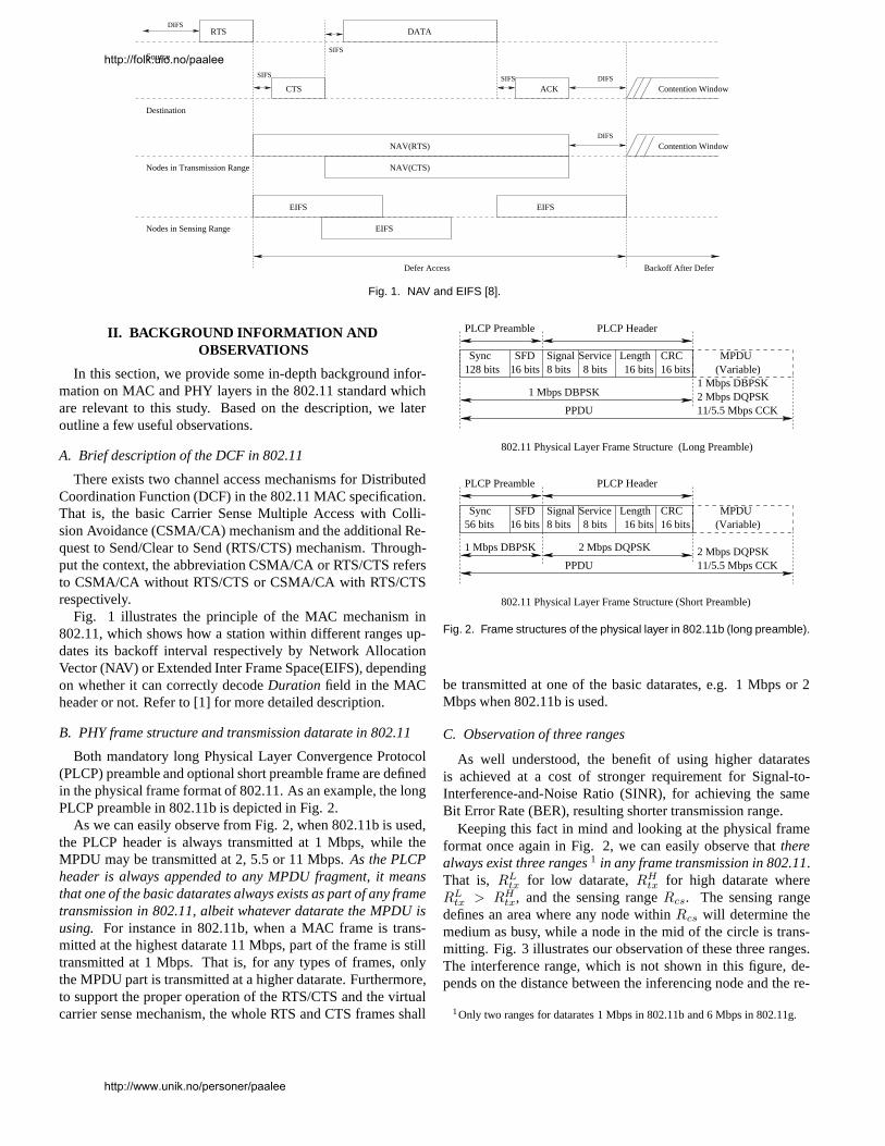
Fig. 1. NAV and EIFS [8].

II. BACKGROUND INFORMATION ANDOBSERVATIONS

In this section, we provide some in-depth background infor-mation on MAC and PHY layers in the 802.11 standard whichare relevant to this study. Based on the description, we lateroutline a few useful observations.

A. Brief description of the DCF in 802.11

There exists two channel access mechanisms for DistributedCoordination Function (DCF) in the 802.11 MAC specification.That is, the basic Carrier Sense Multiple Access with Colli-sion Avoidance (CSMA/CA) mechanism and the additional Re-quest to Send/Clear to Send (RTS/CTS) mechanism. Through-put the context, the abbreviation CSMA/CA or RTS/CTS refersto CSMA/CA without RTS/CTS or CSMA/CA with RTS/CTSrespectively.

Fig. 1 illustrates the principle of the MAC mechanism in802.11, which shows how a station within different ranges up-dates its backoff interval respectively by Network AllocationVector (NAV) or Extended Inter Frame Space(EIFS), dependingon whether it can correctly decode Duration field in the MACheader or not. Refer to [1] for more detailed description.

B. PHY frame structure and transmission datarate in 802.11

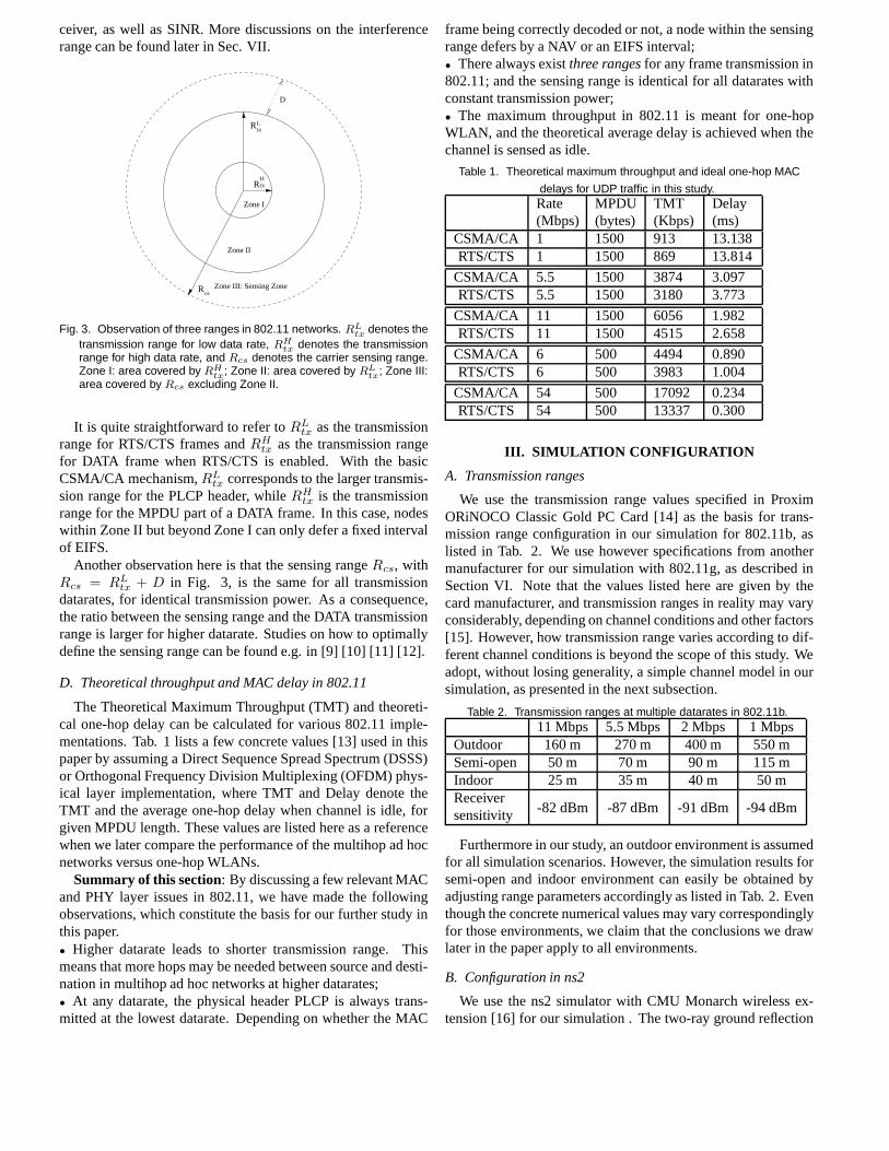
Both mandatory long Physical Layer Convergence Protocol(PLCP) preamble and optional short preamble frame are definedin the physical frame format of 802.11. As an example, the longPLCP preamble in 802.11b is depicted in Fig. 2.

As we can easily observe from Fig. 2, when 802.11b is used,the PLCP header is always transmitted at 1 Mbps, while theMPDU may be transmitted at 2, 5.5 or 11 Mbps. As the PLCPheader is always appended to any MPDU fragment, it meansthat one of the basic datarates always exists as part of any frametransmission in 802.11, albeit whatever datarate the MPDU isusing. For instance in 802.11b, when a MAC frame is trans-mitted at the highest datarate 11 Mbps, part of the frame is stilltransmitted at 1 Mbps. That is, for any types of frames, onlythe MPDU part is transmitted at a higher datarate. Furthermore,to support the proper operation of the RTS/CTS and the virtualcarrier sense mechanism, the whole RTS and CTS frames shall

1 Mbps DBPSK 2 Mbps DQPSK 11/5.5 Mbps CCK

16 bits128 bitsSync SFD

16 bits 16 bitsSignal Length8 bits 8 bits

PLCP HeaderPLCP Preamble

1 Mbps DBPSK

PPDU

CRC(Variable)MPDU

2 Mbps DQPSK 11/5.5 Mbps CCK

16 bitsSync SFD

16 bits 16 bitsSignal Length8 bits 8 bits

PLCP HeaderPLCP Preamble

PPDU

CRC(Variable)MPDU

802.11 Physical Layer Frame Structure (Long Preamble)

802.11 Physical Layer Frame Structure (Short Preamble)

56 bits

1 Mbps DBPSK 2 Mbps DQPSK

Service

Service

Fig. 2. Frame structures of the physical layer in 802.11b (long preamble).

be transmitted at one of the basic datarates, e.g. 1 Mbps or 2Mbps when 802.11b is used.

C. Observation of three ranges

As well understood, the benefit of using higher dataratesis achieved at a cost of stronger requirement for Signal-to-Interference-and-Noise Ratio (SINR), for achieving the sameBit Error Rate (BER), resulting shorter transmission range.

Keeping this fact in mind and looking at the physical frameformat once again in Fig. 2, we can easily observe that therealways exist three ranges 1 in any frame transmission in 802.11.That is, RL

tx for low datarate, RHtx for high datarate where

RLtx > RH

tx, and the sensing range Rcs. The sensing rangedefines an area where any node within Rcs will determine themedium as busy, while a node in the mid of the circle is trans-mitting. Fig. 3 illustrates our observation of these three ranges.The interference range, which is not shown in this figure, de-pends on the distance between the inferencing node and the re-

1Only two ranges for datarates 1 Mbps in 802.11b and 6 Mbps in 802.11g.

http://folk.uio.no/paalee

http://www.unik.no/personer/paalee

http://folk.uio.no/paalee

http://www.unik.no/personer/paalee

242

ceiver, as well as SINR. More discussions on the interferencerange can be found later in Sec. VII.

Rtx

Rtx

Rcs

H

L

Zone I

Zone II

Zone III: Sensing Zone

D

Fig. 3. Observation of three ranges in 802.11 networks. RLtx

denotes thetransmission range for low data rate, RH

txdenotes the transmission

range for high data rate, and Rcs denotes the carrier sensing range.Zone I: area covered by RH

tx; Zone II: area covered by RL

tx; Zone III:

area covered by Rcs excluding Zone II.

It is quite straightforward to refer to RLtx as the transmission

range for RTS/CTS frames and RHtx as the transmission range

for DATA frame when RTS/CTS is enabled. With the basicCSMA/CA mechanism, RL

tx corresponds to the larger transmis-sion range for the PLCP header, while RH

tx is the transmissionrange for the MPDU part of a DATA frame. In this case, nodeswithin Zone II but beyond Zone I can only defer a fixed intervalof EIFS.

Another observation here is that the sensing range Rcs, withRcs = RL

tx + D in Fig. 3, is the same for all transmissiondatarates, for identical transmission power. As a consequence,the ratio between the sensing range and the DATA transmissionrange is larger for higher datarate. Studies on how to optimallydefine the sensing range can be found e.g. in [9] [10] [11] [12].

D. Theoretical throughput and MAC delay in 802.11

The Theoretical Maximum Throughput (TMT) and theoreti-cal one-hop delay can be calculated for various 802.11 imple-mentations. Tab. 1 lists a few concrete values [13] used in thispaper by assuming a Direct Sequence Spread Spectrum (DSSS)or Orthogonal Frequency Division Multiplexing (OFDM) phys-ical layer implementation, where TMT and Delay denote theTMT and the average one-hop delay when channel is idle, forgiven MPDU length. These values are listed here as a referencewhen we later compare the performance of the multihop ad hocnetworks versus one-hop WLANs.

Summary of this section: By discussing a few relevant MACand PHY layer issues in 802.11, we have made the followingobservations, which constitute the basis for our further study inthis paper.• Higher datarate leads to shorter transmission range. Thismeans that more hops may be needed between source and desti-nation in multihop ad hoc networks at higher datarates;• At any datarate, the physical header PLCP is always trans-mitted at the lowest datarate. Depending on whether the MAC

frame being correctly decoded or not, a node within the sensingrange defers by a NAV or an EIFS interval;• There always exist three ranges for any frame transmission in802.11; and the sensing range is identical for all datarates withconstant transmission power;• The maximum throughput in 802.11 is meant for one-hopWLAN, and the theoretical average delay is achieved when thechannel is sensed as idle.

Table 1. Theoretical maximum throughput and ideal one-hop MAC

delays for UDP traffic in this study.Rate(Mbps)

MPDU(bytes)

TMT(Kbps)

Delay(ms)

CSMA/CA 1 1500 913 13.138RTS/CTS 1 1500 869 13.814

CSMA/CA 5.5 1500 3874 3.097RTS/CTS 5.5 1500 3180 3.773

CSMA/CA 11 1500 6056 1.982RTS/CTS 11 1500 4515 2.658

CSMA/CA 6 500 4494 0.890RTS/CTS 6 500 3983 1.004

CSMA/CA 54 500 17092 0.234RTS/CTS 54 500 13337 0.300

III. SIMULATION CONFIGURATION

A. Transmission ranges

We use the transmission range values specified in ProximORiNOCO Classic Gold PC Card [14] as the basis for trans-mission range configuration in our simulation for 802.11b, aslisted in Tab. 2. We use however specifications from anothermanufacturer for our simulation with 802.11g, as described inSection VI. Note that the values listed here are given by thecard manufacturer, and transmission ranges in reality may varyconsiderably, depending on channel conditions and other factors[15]. However, how transmission range varies according to dif-ferent channel conditions is beyond the scope of this study. Weadopt, without losing generality, a simple channel model in oursimulation, as presented in the next subsection.

Table 2. Transmission ranges at multiple datarates in 802.11b.11 Mbps 5.5 Mbps 2 Mbps 1 Mbps

Outdoor 160 m 270 m 400 m 550 mSemi-open 50 m 70 m 90 m 115 mIndoor 25 m 35 m 40 m 50 mReceiversensitivity -82 dBm -87 dBm -91 dBm -94 dBm

Furthermore in our study, an outdoor environment is assumedfor all simulation scenarios. However, the simulation results forsemi-open and indoor environment can easily be obtained byadjusting range parameters accordingly as listed in Tab. 2. Eventhough the concrete numerical values may vary correspondinglyfor those environments, we claim that the conclusions we drawlater in the paper apply to all environments.

B. Configuration in ns2

We use the ns2 simulator with CMU Monarch wireless ex-tension [16] for our simulation . The two-ray ground reflection

243

model is used as the propagation model and omnidirectional an-tenna with unit gain is assumed for both transmitter and receiver.The radio parameters in 802.11b simulation configuration arelisted in Tab. 3.

Table 3. Radio parameters used in 802.11b simulation.

Antenna height 1.5 meterCarrier frequency 2452 MHzTransmission power 15 dBmCPThreshold 10CSThreshold 9.5421× 10−13 (Rcs = 640 m)

1.17× 10−10 (11 Mbps)

RXThreshold 3.0123× 10−11 (5.5 Mbps)6.2535× 10−12 (2 Mbps)1.7495× 10−12 (1 Mbps)

The transmission power is always set as 15 dBm in oursimulation, and corresponding transmission ranges at differentdatarates are achieved by adjusting the receiving threshold (RX-Threshold in ns2). Indeed, fixed transmission power is one ofthe fundamental assumptions in this study and energy consump-tion at each node at different datarates is not within the interestof this paper.

Furthermore, the three range observation presented earlier hasbeen implemented in our ns2 codes. The sensing range is setas 640 meters in our 802.11b simulations, leading to the ratiosbetween Rcs and RH

tx as 4, 2.37, 1.6 or 1.16 at 11, 5.5, 2 or 1Mbps respectively. All simulation results shown in this paperare obtained with a simulation time of 100 seconds. The queuein each node is a First In First Out (FIFO) queue with tail drop,and the queue length is 50 packets. The Ad hoc On DemandDistance Vector (AODV) protocol [17] is chosen as the routingprotocol for scenarios in Sections IV and V, and the OptimizedLink State Routing (OLSR) [18] is used for scenarios in SectionVI respectively. No priority is given to protocol packets.

Both Constant Bit Rate (CBR)/User Datagram Protocol(UDP) and File Transfer Protocol (FTP)/Transmission ControlProtocol (TCP) traffic are considered in this study. More detailson traffic generation can be found later in the paper.

C. Simulation scenarios

Table 4. Simulation scenarios: two for static chain topology and two for

nodes with or without mobility respectively.d 11 Mbps 5.5 Mbps 2 Mbps 1 Mbps

Scen. I 150 m 12 hops 12 hops 6 hops 4 hopsScen. II 125 m 12 hops 6 hops 4 hops 3 hopsScen. III 100 nodes with mobility in a 1200× 1200 m2 areaScen. IV 100 stationary nodes in a 800 × 800 m2 area [20]

Four scenarios are considered in our study, where the firsttwo are based on a chain topology with stationary nodes whilethe third and the fourth deal with nodes located in two dimen-tional areas, with or without mobility respectively. The basicfeatures of the considered scenarios are listed in Tab. 4. Withchain topology, there is only one traffic flow in the network, ini-tiating at node 0 and terminating at node 12 or node 6. Note thatfor both static and mobile scenarios, we consider that all nodes

along a source-destination path are using the same datarate andthe datarate does not change during simulation lifetime. Thisassumption is reasonable given the fact that the performance of802.11 is greatly degraded if different datarates are used at thesame time within the one-hop vicinity [19].

The chain topology is shown in Fig. 4. The distance betweenany two immediate neighboring nodes, denoted as d, is identicalfor all neighbor-pairs. Depending on the different transmissionranges listed in Tab. 2, the number of hops between source anddestination varies at each datarate.

d

node 0 node 1 node 2 node 12node 11node 10

Fig. 4. 13 nodes in chain topology. The distances between any twoneighboring nodes are identical and equal to d meters. Only onesource traffic flow from node 0 to node 12.

Scenario III in our study deals with multihop networks in amesh topology with node mobility. 100 nodes are placed in asquare area of 1200×1200m2. The stationary random waypointmodel is employed as the mobility model in this study [21]. Twotraffic patterns are generated in this scenario: 1) Homogeneoustraffic, 4 CBR/UDP flows each at source bitrate 200 Kbps; 2)Heterogeneous traffic, 4 FTP/TCP connections are generated,in addition to 4 CBR/UDP traffic flows. The TCP agent usedis the Base TCP Sender (Tahoe TCP) with congestion controland round-trip-time estimation. The TCP packets are of length1000 bytes, and the window size is set as 4. Among all nodesin the area, 8 or 16 nodes are arbitrarily chosen as the sourceand destination nodes respectively in these two cases, and othernodes only act as relays when necessary.

Scenario IV focuses on performance of 802.11g based mul-tihop networks with static uniform node distribution, where therelationship between datarate and network connectivity has beenstudied in depth.

IV. NUMERICAL RESULTS FOR CHAIN TOPOLOGY

This section presents and discusses the simulation results wehave obtained based on the scenarios for chain topology as de-scribed above.

A. Maximum chain throughput at multirates

The authors in [22] concluded that the chain throughput inmultihop ad hoc networks is 1/4 ∼ 1/7 of the maximum one-hop throughput (TMT), using the default ranges in ns2 as Rtx =250 m and Rcs = 550 m. In this subsection, we investigatethe maximum chain throughput at each datarate, based on ourobservations in Sec. II. A salient distinction between this studyand the work in [22] is: the fact that lower datarate leads toshorter path, and vice versa, has been considered in this paper.

The purpose of this set of simulations is to find the maximumthroughput in a multihop ad hoc network. So for all curves il-lustrated in Figs. 5 - 8, the traffic bitrate generated at the sourcenode is slightly higher than the corresponding one-hop TMTslisted in Tab. 1. By doing so, there are always packets ready fortransmission at the source node. In other words, the throughput

244

0 2 4 6 8 10 120

1000

2000

3000

4000

5000

6000

7000

Chain Length (Node Number)

Cha

in T

hrou

ghpu

t at D

iffe

rent

Dat

arat

e (K

bps)

UDP traffic, CSMA/CA

d = 150 m, datarate = 11 Mbps, 1500 bytesd = 150 m, datarate = 5.5 Mbps, 1500 bytesd = 150 m, datarate = 2 Mbps, 1500 bytesd = 150 m, datarate = 1 Mbps, 1500 bytes

Fig. 5. Scenario I: maximum throughput for multihop ad hoc networks atdifferent data rates. CBR/UDP traffic with CSMA/CA. The number ofhops for data rate 11, 5.5, 2 or 1 Mbps is 12, 12, 6, or 4 respectively.

0 2 4 6 8 10 120

500

1000

1500

2000

2500

3000

3500

4000

4500

5000


Cha

in T

hrou

ghpu

t at D

iffe

rent

Dat

arat

e (K

bps)

UDP traffic, RTS/CTS


Fig. 6. Scenario I: maximum throughput for multihop ad hoc networks atdifferent data rates. CBR/UDP traffic with RTS/CTS. The number ofhops for data rate 11, 5.5, 2 or 1 Mbps is 12, 12, 6, or 4 respectively.

simulated in these figures is the saturation throughput for mul-tihop networks 2. Another worthy point to mention here is thatsince the source rate is generated higher than the TMT and thethroughput at the destination node is much lower than the TMT,the overall packet loss ratio could be very high (> 90% at 11Mbps with RTS/CTS) in this set of simulations.

Now let us illustrate and discuss the simulation results shownin Figs. 5 - 8. For each scenario listed in Tab. 4, we havesimulated the performance of a chain topology ad hoc networkfor both CSMA/CA and RTS/CTS mechanisms. The results forScenario I are depicted in Figs. 5 and 6, and the correspondingresults for Scenario II are shown in Figs. 7 and 8. In fact, thedifference between these two scenarios, i.e., different distancebetween neigboring nodes, has also led to a spin-off result onchain topology throughput, as explained later in this subsection.

The first impression we get from these figures is thateven though the one hop TMT varies greatly as the dataratechanges, the difference between chain throughput among var-

2Of course, the nodes closer to the destination may not be saturated, but onecannot send higher bitrate at the source node. Or, higher source rate would notresult in a higher chain throughput at the destination.

0 2 4 6 8 10 120

1000

2000

3000

4000

5000

6000

7000


Cha

in T

hrou

ghpu

t at D

iffe

rent

Dat

arat

e (K

bps)



Fig. 7. Scenario II: maximum throughput for multihop ad hoc networksat different data rates. CBR/UDP traffic with CSMA/CA. The numberof hops for data rate 11, 5.5, 2 or 1 Mbps is 12, 6, 4, or 3 respectively.

0 2 4 6 8 10 120

500

1000

1500

2000

2500

3000

3500

4000

4500

5000


Cha

in T

hrou

ghpu

t at D

iffe

rent

Dat

arat

e (K

bps)



Fig. 8. Scenario II: maximum throughput for multihop ad hoc networksat different data rates. CBR/UDP traffic with RTS/CTS. The numberof hops for data rate 11, 5.5, 2 or 1 Mbps is 12, 6, 4, or 3 respectively.

ious datarates shrinks rapidly as the chain length grows. Forexample, when the chain length is 6 hops, the throughput for 11Mbps datarate is at most twice as high as that for 1 Mbps, for allsimulated cases. This is a remarkable contrast with the differ-ence between the raw transmission datarates (11 Mbps versus 1Mbps), and the one-hop TMT (∼ 6 times difference between 11and 1 Mbps in Tab. 1).

Let us examine the figures more carefully now. ForCSMA/CA, Fig. 5 shows that there is a visible throughput dif-ference among different datarates at quite long path. For anotherdistance configuration shown in Fig. 7, there is almost no dif-ference in chain throughput between datarates 5.5 and 11 Mbpswhen the chain length is larger than 6. Anyhow with CSMA/CA,the chain throughput for high datarates is still higher than that oflow datarates. However, when RTS/CTS is enabled, the distinc-tion disappears very soon. Figs. 6 and 8 illustrate that the chainthroughput for all data rates is almost the same, once the chainlength is 6 hops or more. To conclude, there is almost no gainin applying high datarate in multihop ad hoc networks when thechain length is 6 hops or more.

Moreover, this conclusion does not imply that using 11 Mbps

245

200 400 600 800 1000 1200

200

400

600

800

1000

1200

Source Bitrate (Kbps)

Cha

in T

hrou

ghpu

t for

Sce

nari

o II

(K

bps)


7 nodes in chain topology, d = 125 m

datarate = 11 Mbps, 6 hopsdatarate = 5.5 Mbps, 3 hopsdatarate = 2 Mbps, 2 hopsdatarate = 1 Mbps, 2 hops

Fig. 9. Chain throughput for multihop ad hoc networks at different datarates with CSMA/CA (Scenario II). Moderate CBR/UDP traffic. Thenumber of hops for data rate 11, 5.5, 2 or 1 Mbps is 6, 3, 2, or 2respectively.

is beneficial for chain length less than 6 either. Look at the re-sults for Scenario II in Figs. 7 and 8 as an example. The through-put for 11 Mbps drops so sharply that 5.5 Mbps has achievedindeed higher throughput when chain length is of 2 ∼ 6 hops.This is simply because that the path length at 5.5 Mbps is onlyone half of that at 11 Mbps in this case.

The above results show that the benefit of using high dataratediminishes as path length increases. This is because that theoverhead in 802.11 is comparatively heavier at higher datarate,and as path length grows, the overhead is incurred more andmore times, resulting in a diminished gain from high datarate.With RTS/CTS, the per-hop overhead is even heavier. The chainthroughput with RTS/CTS thus converges more tightly at longchain length, since this even-heavier per-hop overhead has to berepeated several times at multihop.

Here we would also like to present a spin-off result on chainthroughput for single datarate, as an enhancement to the con-clusion in [22]. Take 11 Mbps as an example, as shown in Figs.5-6. Depending on which mechanism is used, the chain through-put achieved at node 12 is less than 1/10 or 1/20 of the one-hopTMT, for CSMA/CA or RTS/CTS respectively. (Note that thisconclusion is independent of which datarate is used.) What weobserve here is substantially lower than the result they reported.However, the reason for this result is simple: with shorter dis-tance between neighboring nodes, more nodes take part in chan-nel contention, since now more nodes are covered by the sameinterference range. More specifially with our distance configu-ration, only nodes which are 5- or 6-hops away from each othercan transmit simultaneously. With RTS/CTS enabled, this effectis more serious since the CTS frames sent by the receiver canreach even further.

B. Performance at moderate traffic load

In this subsection, with a more realistic scheme, we continueto study the performance of the multihop networks, at moder-ate traffic loads. The distinction from the maximum through-put study above is that, with moderate traffic load, we are ableto identify a range of network ’supportable’ source bitrates thatexperiences high throughput, low delay and low packet loss in

200 400 600 800 1000 1200100

200

300

400

500

600

700

800

900

1000


Cha

in T

hrou

ghpu

t for

Sce

nari

o II

(K

bps)




Fig. 10. Chain throughput for multihop ad hoc networks at different datarates with RTS/CTS (Scenario II). Moderate CBR/UDP traffic. Thenumber of hops for data rate 11, 5.5, 2 or 1 Mbps is 6, 3, 2, or 2respectively.

the network, for each datarate. To conduct this experiment, thesource bitrate is set as 1200, 1000, 800, 400, or 200 Kbps re-spectively for the same packet length.

Having concluded from the above subsection that the benefitof using 11 Mbps disappears with path length of 6 hops, wecontinue the study on chain topology with only 7 nodes here.The number of hops between source and destination becomes 6,3, 2, or 2 at 11, 5.5, 2 or 1 Mbps correspondingly. Scenario II inTab. 4 is employed in this set of simulations.

B.1 Achievable chain throughput

Ideally, the network should be able to provide a quite linearthroughput curve at moderate load. The problem is that as thechain length increases, the multihop network soon becomes sat-urated. Figs. 9 and 10 illustrate the chain throughput achievedat node 6, for CSMA/CA and RTS/CTS respectively. Using thesource bitrate as the horizontal axes, the figures show when thenetwork becomes saturated, at each datarate. 5.5 Mbps achievesthe highest ’supportable’ source rate, with both mechanisms. In-terestingly with RTS/CTS, the supportable bitrate at 11 Mbpshas decreased even below that of 2 Mbps. However, it is notvery surprising if we notice that the path length at 2 Mbps isonly one third of that at 11 Mbps. The 3-time TMT benefit by11 versus 2 Mbps has been counteracted by the 3-time longerpath.

B.2 End-to-end delay

Figs. 11 and 12 illustrate the ETE delay results withCSMA/CA and RTS/CTS respectively, with a logarithmic ver-tical axis. Even though the one-hop delay is much shorter at11 Mbps, the difference becomes smaller as the chain lengthincreases. Once the channel becomes saturated, the ETE delaysjump dramatically to hundreds of milliseconds, or even seconds,level for all datarates.

In summary, in this subsection we have investigated the per-formance of an 802.11b based multihop ad hoc network in chaintopology, at relatively moderate network load. There are a fewquite interesting observations in the context. Firstly, when thetraffic load is very light (< 400 Kbps), the source application

246

200 400 600 800 1000 120010

−2

10−1

100


End

−to

−en

d de

lay

(sec

) UDP traffic, CSMA/CA



Fig. 11. End-to-end delay for multihop ad hoc networks at different datarates with CSMA/CA. Moderate CBR/UDP traffic. The number ofhops for data rate 11, 5.5, 2 or 1 Mbps is 6, 3, 2, or 2 respectively.

200 400 600 800 1000 1200

10−1

100


End

−to

−en

d de

lay

(sec

) UDP traffic, RTS/CTS



Fig. 12. End-to-end delay for multihop ad hoc networks at different datarates with RTS/CTS. Moderate CBR/UDP traffic. The number ofhops for data rate 11, 5.5, 2 or 1 Mbps is 6, 3, 2, or 2 respectively.

can enjoy ’guaranteed’ service for all concerned performanceparameters (i.e., chain throughput, ETE delay and packet lossratio) at any datarate. In this case, a sender would probably pre-fer to use datarates 1 or 2 Mbps to reduce the number of hopsto destination, if the intrinsic transmission delay at low datarateis tolerable for the application. Secondly, for a medium traf-fic load (around 400− 800 Kbps), the higher datarates achievebetter performance than their lower datarate counterparts. How-ever in this case, one would probably like to use 5.5 Mbps,not 11 Mbps, since it provides both ’guaranteed’ performanceand shorter number of hops. Finally, when the traffic load iscomparatively heavy (> 1000 or 1200 Kbps for RTS/CTS orCSMA/CA respectively), there is no convincing performance atall, at any datarate. Why should we use high datarate even inthis case? As a means to avoid network congestion, one wouldprefer to introduce rate control at the source node. However,that is outside the scope of this paper.

V. NUMERICAL RESULTS WITH NODE MOBILITY

This section presents and discusses the simulation resultsbased on a mesh topology with node mobility. To make a statis-tically more accurate observation on the performance of the con-cerned network, we generate a set of 10 diverse mobility patternsfor each mobility configuration. Each configuration corresponds

to an identical setting of average speed, pause time etc. For in-stance, for the same average velocity of 5 m/s and pause timeof 10 sec used in our simulations, the nodes move according to10 different trajectories. The simulation results to be illustratedbelow are the average values from 10 mobility patterns.

We have mentioned earlier that the number of hops betweensource and destination nodes listed in Tab. 4 is only an ’ideal’value for stationary chain topology. In reality, this number, aswell as the routing path, is decided by the routing protocol be-ing used, and the routing protocol may choose more hops thanthe ideal number of hops. Therefore, it is of interest to investi-gate the number of hops at different datarates, especially whennodes are moving, since path length may vary from time to timedue to mobility. In addition to the number of hops, we are alsoinvestigating other parameters, the average throughput, end-to-end delay and packet loss ratio in this section. Furthermore, wehave run two sets of simulations, with CSMA/CA or RTS/CTS,for this scenario. However, we present only simulation resultswith CSMA/CA in this section.

A. Average and maximum numbers of hops

Tab. 5 lists the experienced average and maximum numberof hops at each datarate, for homogeneous traffic pattern. HereNave

hops and Nmaxhops denote the average and the maximum numbers

of hops respectively.

Table 5. Average and maximum number of hops at different datarates.

Averaged from 4 pure CBR/UPD flows.11 Mbps 5.5 Mbps 2 Mbps 1 Mbps

Navehops 4.2 2.7 1.9 1.2

Nmaxhops 15.1 8.4 7.4 5.7

Nneighbor 6.0 15.9 34.9 66.0

As expected, the simulation results on the number of hopscoincide with our intuitive impression from chain topology inSec. III. That is, higher datarate leads to higher number of hops.Moreover, even though the average number of hops is quite lowas shown in the table, some paths may be very long. As twoextreme cases, Fig. 13 further illustrates the distributions of thenumber of hops at datarates 1 and 11 Mbps respectively. At 1Mbps, a majority of destinations are directly reachable by thesource nodes. It is sparsely in this case that a path would belonger than 4 hops. At 11 Mbps, on the other hand, many pack-ets may need to transfer over multiple hops, even up to 15 hops.Although there is only a small minority of packets with verylong paths, those ’misbehaved’ packets deteriorate the overallperformance significantly, e.g., to the average ETE delays aswill be shown later.

Recall the 6-hop conclusion obtained from chain topologyearlier and notice that the average number of hops at 11 Mbps isonly 4.2 in this case. One might expect that 11 Mbps performsbetter than other datarates. However, as will be illustrated below,the benefit of using high datarate diminishes at even shorter pathlength when the mesh topology with node mobility is involved.

B. Average throughput

The simulation results on average throughput for both trafficpatterns are tabulated in 6, where a successfully received packetmay need from 1 to Nmax

hops hops to reach the destination.

247

0 2 4 6 8 10 12 14 16 180

2

4

6

8

10

12

14

16x 10

4

Average number of hops

Dis

trib

utio

n of

the

aver

age

num

ber

of h

ops

Pure CBR/UDP traffic, Source rate = 4*200 Kbps

<== Datarate = 1 Mbps

<== Datarate = 11 Mbps

Fig. 13. Histogram showing the distribution of the number of hops atdatarates 11 and 1 Mbps, for pure UDP traffic.

As shown in the table, the achieved average throughput is re-ally not satisfactory, for both traffic patterns. With pure UDPtraffic, only 5.5 Mbps managed to provide 90% of the requiredbandwidth, and the throughput achieved at 11 Mbps is evenlower than that at 2 Mbps. When heterogeneous traffic where4 UDP and 4 TCP flows co-exist, however, 5.5 Mbps can onlyachieve about 2/3 of the required bandwidth, while only half ofthe required bandwidth is obtained at 11 and 2 Mbps. 1 Mbpsperforms worst in both cases due to its intrinsic datarate limita-tion. In the heterogeneous case, the rest of the used bandwidthis absorbed TCP traffic.

Table 6. Average throughput/goodput for UDP and TCP flows, in Kbps.

Homogeneous 11 Mbps 5.5 Mbps 2 Mbps 1 MbpsUDP 133.9 180.0 149.3 123.5

Heterogeneous 11 Mbps 5.5 Mbps 2 Mbps 1 MbpsUDP 102.3 137.3 100.7 66.7TCP 372.8 522.6 390.0 267.0

The reason that TCP flows achieve higher throughput thanUDP flows is due to TCP’s capability to adjust its source rateaccording to network congestion status. Fig. 14 illustrates howTCP behaves against simulation time. Generally TCP tries tosend more packets when the network is less congested, andvice versa. There are also periods in which TCP traffic is fullystopped. This adaptivity gives TCP traffic high throughput anda very low packet loss, as will also be shown later.

In general, 5.5 Mbps performs best with node mobility, forboth UDP and TCP traffic. This implies that, with the parame-ters settings used in this study, the tradeoff between the numberof hops and chain throughput is optimally achieved at datarate5.5 Mbps, for the studied 802.11b multihop network.

C. End-to-end delay

The average, minimum and maximal end-to-end delays sim-ulated are tabulated in Tab. 7, denoted by Dave, Dmin, andDmax respectively. We also list in the table the percentage ofthe successfully received packets that have ETE delays shorterthan 250 ms, corresponding to the radio access bearer transferdelay for streaming traffic class defined in [23]. The end-to-enddelays in the context include also accumulated queueing delaysat all intermediate node(s).

0 10 20 30 40 50 60 70 80 90 1000

200

400

600

800

1000

1200

Simulation Time (sec)

TC

P T

hrou

ghpu

t Exp

erie

nced

ove

r T

ime

(Kbp

s)

Datarate = 11 Mbps, average of 4 TCP flows

Fig. 14. Average TCP throughput over time, for heterogeneous trafficpattern. Datarate = 11 Mbps. TCP traffic starts at second 4.

The minimum delays represent the situation where the des-tination nodes are only one hop away from the source nodes,and the packets ’luckily’ acquire the channel immediately whenready. However, even in the one-hop case, a packet may haveto wait in the queue at the source node before it is transmit-ted. Moreover, as illustrated from hop distribution, many pack-ets have to transfer several hops before they reach the destina-tion. In extreme cases, packets may have to wait up to severalhundred of milliseconds or even seconds in the buffers at variousnodes before they reach their destinations. This leads to a verylong maximum delay in ranges of seconds, at all datarates. Wehave observed from the simulation results that, compared withthe backoff and transmission delays, the queueing delay domi-nates the end-to-end delay in multihop ad hoc networks.

Table 7. End-to-end delays at different datarates.

Homogeneous 11 Mbps 5.5 Mbps 2 Mbps 1 MbpsDave 315 ms 102 ms 415 ms 571 msDmin 1.4 ms 1.2 ms 2.4 ms 4.5 msDmax 14.6 sec 10.5 sec 7.6 sec 5.8 sec

PD<250ms 79% 93% 73% 60%

Heterogeneous 11 Mbps 5.5 Mbps 2 Mbps 1 MbpsDave

UDP553.0 ms 701.2 ms 995.3 ms 1795 ms

PD<250ms 63% 51% 43% 21%

DaveTCP

90.6 ms 78.7 ms 85.0 ms 139.0 msPD<250ms 93% 99% 95% 89%

0 100 200 300 400 500 600 700 800 900 10000

0.5

1

1.5

2

2.5

3

3.5

4

4.5x 10

4

End−to−End Delay (ms) in 20 ms Interval

Del

ay H

isto

gram

Datarate = 11 Mbps, Pure CBR/UDP traffic

Source rate = 4*200 Kbps

Fig. 15. Histogram showing the distribution of the end-to-end delay at11 Mbps, for pure UDP traffic.

248

Furthermore, Fig. 15 illustrates the distribution of the ETEdelay at 11 Mbps for homogeneous traffic. In this example, only68% of the successful packets can enjoy short delay of ≤ 100ms, while 8% packets have experienced long delay of over 1second. (The peak at the right-most point in the figure includesall packets with delay equal to or longer than 1 second).

D. Packet loss

Tab. 8 illustrates the simulated results on total packet loss ra-tio at different channel datarates, for both traffic patterns. As ex-pected, higher packet loss happens to UDP traffic since the sameamount of packets are generated at the source nodes, regardlessof channel condition and network traffic load. With TCP traf-fic, however, the source nodes can adjust its bitrate accordingly,resulting in a very low TCP packet loss, at all datarates.

Table 8. Packet loss at different datarates for two traffic patterns.

Homogeneous 11 Mbps 5.5 Mbps 2 Mbps 1 MbpsUDP 33% 9% 25% 39%

Heterogeneous 11 Mbps 5.5 Mbps 2 Mbps 1 MbpsUDP 48% 32% 49% 66%TCP 2.0% 1.7% 1.7% 2.3%

VI. NUMERICAL RESULTS FOR 802.11G NETWORKS

In this section, we present briefly another set of simulationresults which are based on 802.11b/g based multihop wirelessnetworks. More detailed information about this scenario andnumerical results can be found in [20].

Basically for this scenario, we generate 100 static nodes uni-formly distributed in a square area of 800×800 m2. 6 dataratesare selected as the candidate datarates for our performance eval-uation, which are 54 Mbps, 36 Mbps, 18 Mbps, 11 Mbps, 6Mbps, and 1 Mbps, with corresponding transmission ranges as76 m, 130 m, 183 m, 304 m, 396 m and 610 m respectively, ac-cording the Cisco Aironet Card specification [24]. It is worthymentioning that due to the consideration that the later proposedrate adaptation algorithm in Subsection VII-C requires networktopology information, OLSR has been chosen as the routing pro-tocol for this scenario. With its proactive feature, OLSR pro-vides us with necessary network topology and neighbor connec-tion information beforehand no matter there exists any any datatraffic or not in the studied network.

A. Topology and routing information using OLSR

We study network connectivity first in this scenario. Withthis perspective, the most important two performance observa-tions are: 1) How many destinations can be reached by the rout-ing protocol, among all nodes distributed in the area, at eachdatarate; and, 2) How long would the routing path be, on aver-age and at maximal, in number of hops, at each datarate. Thesimulation results are summarized in Tab. 9, where Routeest

means the average number of routes established, Hopave andHopmax indicate the average and maximum path lengths forthe established routes. As a reference, the average number ofneighbors at each datarate, Neighborave, is also listed in thetable.

Since there are totally 100 nodes in the network, the Routeest

value would be 99 if all other nodes are reachable. The simu-

Table 9. Topology and routing information obtained by OLSR.

Datarate (Mbps) 54 36 18 11 6 1Routeest 14 95 99 99 99 99Hopave 2.7 5.3 3.2 2.0 1.5 1.2Hopmax 5.3 9.5 5.9 4.8 2.6 2

Neighborave 3.4 6.2 13.2 33.4 47.0 82.3

lation results in Table 9 show that only datarates equal to orlower than 18 Mbps can achieve full connectivity. At 36 Mbps,routes to around 5% nodes cannot be established, thus select-ing 36 Mbps as the ’working’ datarate would be ’risky’ fromthe perspective of full connectivity. Not surprisingly, datarate54 Mbps provides very poor connectivity and this counteractsgreatly with its advantage of high per-link capacity.

B. End-to-end delay and packet loss for UDP traffic

Among the 100 nodes uniformly distributed within the area,20 nodes are arbitrarily chosen as 10 source-destination pairs.To avoid packet loss earlier observed at heavy traffic load, onlylight traffic load is generated for CBR/UDP traffic in this simu-lation. This implies that most packets experience mainly MACdelay and transmission delay over multihops. More specificallyin this case, the CBR traffic generated at each source node is 40Kbps, where the packet length is 500 bytes.

Table 10. End-to-end delay and packet loss ratio for CBR/UDP traffic.

Datarate (Mbps) 54 36 18 11 6 1DETE

ave (ms) 1.2 5.6 6.6 37.9 72.1 299.0Loss ratio (%) 95 5 0 0.7 2.3 29.8

Throughput (Kbps) 2 38 40 39.7 39.1 28.1

The simulation results shown in Tab. 10 are the averagevalues of 10 flows over 10 different topologies, where DETE

ave

means the average end-to-end delay in milliseconds.The reason that 54 Mbps receives very poor throughput is

quite clear: lack of connectivity. In fact, we observed in sim-ulation that 95% of the generated packets are lost and no-route-to-destination is the only reason for this packet drop. Only infew cases where the destination nodes are geographically quiteclose to the source nodes, the CBR packets can be successfullydelivered, and the average delay for those packets is very lowdue to the intrinsic short per-link delay at 54 Mbps. Otherwisethe generated packets are simply lost, resulting to a very highpacket loss at 54 Mbps. The reason that packet loss is also ob-served at the lowest datarates is that too many HELLO messagesare generated by neighboring nodes especially at 1 Mbps whenalmost all other nodes (82 out of 99) are a node’s one-hop neigh-bors.

C. Throughput, end-to-end delay and packet loss for TCP traffic

Finally, we conduct a set of simulations for FTP/TCP trafficbased on the same network configuration as for CBR traffic. Thesimulation results regarding average throughput, end-to-end de-lay and packet loss are listed in Tab. 11.

Because of TCP’s rate adaptation and retransmission mech-anisms, the packet loss ratio is almost zero once there exists apath between source and destination. However, at the highest

249

two datarates, especially at 54 Mbps, some nodes are isolatedand not reachable due to lack of neighbors. Once those nodesare selected as the source or destination nodes, all packets (a fewpackets) at the starting phase of the corresponding TCP flowsare lost. The TCP connections are not established at all in thesecases. (Note that the loss ratio of around 20% at 54 Mbps listedin the table is the average percentage of the unsuccessful flows,not packets).

Table 11. Throughput, end-to-end delay, and flow loss ratio at each

datarate for TCP traffic.Datarate (Mbps) 54 36 18 11 6 1

Throughput (Kbps) 1124 1016 1953 1742 1570 399DETE

ave (ms) 16.8 30.3 9.2 11.3 21.9 66.2Loss ratio 20.3% < 0.1% 0 0 0 0

The statistics on throughput and end-to-end delays listed inTab. 11 are based on established flows. The end-to-end delaysat different datarates are jointly decided by path length, queue-ing delay, per-link delay and traffic load. At 54 Mbps, manyflows are not established. The total traffic is correspondinglymoderate, resulting in a short queueing delay. A long route isthe main ’contributor’ for the end-to-end delay in this case. At36 Mbps, almost all TCP flows are established. The queueingdelay contributes significantly to the total delay at this datarate.At the lowest two datarates, there are also longer queueing de-lays partly due to more routing overhead mentioned earlier, inaddition to TCP traffic. Of course, the intrinsic long per-link de-lay at lower datarates makes the end-to-end delay even longer inthese cases.

VII. PERFORMANCE ANALYSIS AND AUTOMATICRATE SELECTION ALGORITHM

In the above three sections, we have demonstrated that thehighest datarate(s) do(es) lead to best performance in 802.11based mutihop wireless networks. There are a number of rea-sons that can have impact on this behavior. For example, factorslike channel condition, sensing range, protocol overhead, trafficcharacteristics etc may affect the performance of such multiratenetworks. However, we believe that increased path length andless connectivity, are among others, two major reasons for theperformance degradation at high datarates. Therefore in the fol-lowing subsections, we analyze end-to-end throughput and net-work connectivity in multirate wireless networks first, and then,based on our analytical results, propose an auto-rate selectionalgorithm for such networks.

A. Multihop end-to-end throughput

To make an approximation of the multihop throughput, wefirst calculate the transmitter separation distance, ST−T , basedan interference model [9] [10]. As depicted in Fig. 4, ST−T de-notes the distance in hops between two immediate transmittersthat can transmit simultaneously, and a smaller ST−T indicatesa better spatial reuse.

Given the two-ray propagation model used in this study, thereceived signal strength at the receiver can be simply expressedas [25]

Pr =PtGtGrh

2t h

2r

d4=

C

d4, (1)

where d is the distance between the transmitter and the receiver,and C represents a constant containing transmission power Pt,antenna gains Gt, Gr, and the antenna heights of the transmitterand the receiver ht, hr.

Consider the chain network in Fig. 4 first. The accumulatedsignals from other simultaneous transmitters, which are H hopsaway from transmitter T , are interference to receiver R and canbe calculated as [12]

IRrx =

C

(H − 1)4d4+

C

(H + 1)4d4, (2)

where interference from transmitters that are mH (m ≥ 2) hopsaway from the transmitting node is considered negligible andthus ignored. Symmetrically, the interference at T when R istransmitting an ACK to T is IT

rx = IRrx = C

(H−1)4d4 + C(H+1)4d4 .

Moreover, the background noise can be ignored, assuming aninterference-limited environment. We can thus use Signal-to-Interference Ratio (SIR) to approximate SINR, as follows

SIR1D =Pr

IRrx + IT

rx

=(H2 − 1)4

4(H4 + 6H2 + 1). (3)

Similarly in the two dimensional case, the inference from thesecond tier and further away interfering nodes can be ignored.Thus by considering the first tier 6 nodes in a hexagonal area,the SIR in the 2-D case can be approximated as [11]

SIR2D =1

2(X−1)4

+ 1(X−

1

2)4

+ 1X4 + 1

(X+ 1

2)4

+ 1(X+1)4

,

(4)where X = Rcs

Rtx

is the ratio between the sensing range Rcs andthe transmission range Rtx. It corresponds to ST−T in the 2-D case and defines the minimum distance where simultaneoustransmissions may occur.

Furthermore, to decode a packet correctly, we should haveSIR > ηth, where ηth is the required SIR threshold for eachdatarate. Now the transmitter separation distance ST−T can beobtained as ST−T = min(H) subject to SIR > ηth and Hd >Rcs.

Finally, the end-to-end throughput for multihop networks canbe approximately upper bounded by [10]

ThroughputETE =Throughputper−hop

ST−T=

TMT

ST−T. (5)

Numerically as an example, Tab. 12 lists the calculated ST−T

for 802.11b, where the ηth values are obtained based on Tab. 2and the two-ray propagation model. Note the values for ST−T

used here are for illustration purpose. In practice, these valuesshould be integers.

Table 12. Transmitter separation distance ST−T at different datarates.

Datarate 11 Mbps 5.5 Mbps 2 Mbps 1 Mbpsηth 20.1 dB 15.0 dB 8.2 dB 1.8 dB

ST−T1D 5.1 3.9 2.9 2.4

ST−T2D 5.6 4.2 3.1 2.5

The numerical results in Tab. 12 clearly indicate that the spa-tial reuse at 11 Mbps is much less than that of low datarates,

250

leading to a degraded end-to-end throughput according to Eq.(5). As shown in the table, the throughput degradation at 11Mbps is even worse with mesh topology since there are morenodes within the interference range in the 2-D case. This con-clusion applies to other mutirate multihop 802.11 networks aswell.

B. k-connectivity

Given the same node density, the number of one-hop neigh-bors for each node becomes fewer with shorter transmissionrange, making the network less connected. In the following, wefirst deduce a general formula for calculating the minimum nodedegree by assuming an ideal uniform node distribution, and thendiscuss its effect on average throughput.

Consider a homogeneous Poisson point problem in one di-mension. A number of n nodes where n � 1 are randomlyuniformly positioned in an interval [0, xmax]. The probabil-ity that k of n nodes are placed in the interval [x1, x2], where0 ≤ x1 ≤ x2 ≤ xmax, is given by [26]

P (µ = k) =

(

n

k

)

pk(1− p)n−k, (6)

where µ is a random variable denoting the number of nodeswithin the given interval, and p is the probability that a nodeis placed within the interval [x1, x2], as p = x2−x1

xmax

in the one-dimension case.

With two dimensions, the problem becomes what is the prob-ability that there are k of n nodes distributed within a certainarea of A0, given the total system area as A. Assume om-nidirectional antenna with transmission range r0 and a rectan-gular system area of xmax × ymax. We have A0 = πr2

0 andA = xmaxymax. The probability that there is one node within

the area of A0 is simply p =πr2

0

xmaxymax

.Analogous to the one dimension case, the probability that

there are k nodes distributed within A0 can be obtained by sub-

stituting p =πr2

0

xmaxymax

into Eq. (6). Therefore, the proba-bility that each node has at least k neighbors, i.e., the networkhas a minimum node degree µmin ≥ k, or the network is k-connected, can be calculated by

P (µmin ≥ k) = 1−

k∑

j=0

P (µ = j) (7)

= 1−

k∑

j=0

(

n

j

)

(A0

A)j(1−

A0

A)n−j .

Considering a wireless network in a rectangular area withA = xmax × ymax and each node has an omnidirectional an-tenna with transmission range r, the above expression can easilybe used for calculating k-connectivity by substituting A0 = πr2

and p = A0

A= πr2

xmaxymax

into (7).Numerically, Tables 13 and 14 list the calculated probabilities

of k-connectivity at each datarate in our study for 802.11b (k =3, 6, 10, 15) and 802.11g (k = 6) respectively. Note that theactual node degrees in our simulation with mobility would bebiased due to the border effect and velocity instability problemsin the random waypoint model [27] [28].

Table 13. Probility of k-connectivity for at 802.11b, where n = 100,

xmax = ymax = 1200 meters.

Datarate 11 Mbps 5.5 Mbps 2 Mbps 1 MbpsP (µmin ≥ 3) 81.58% 99.99% 100% 100%P (µmin ≥ 6) 32.54% 99.76% 100% 100%P (µmin ≥ 10) 2.40% 93.62% 100% 100%P (µmin ≥ 15) 0.01% 53.16% 99.99% 100%

Furthermore, identifying the required minimum value of k fora fully connected wireless network is not a trivial task. Earlyresults showed that 6 or 8 as a ’magic number’ for maximalthroughput in a stationary and connected wireless network [29][30]. Smaller [31] or larger number [32] has also been proposedlater as the critical number under different circumstances, e.g.,for stationary or mobile nodes. Another study [33] insisted thatthis value should be related to the total number of nodes insidethe network and proposed to use k = 5.1774logn for provid-ing full connectivity. Through extensitive simulations, we foundthat k = 6 remains as a reasonable number for a static mesh net-work with uniform node distribution. Therefore, k = 6 is usedin our rate adaptation algorithm which is decribed below.

Table 14. Probability of 6-connectivity for 802.11g where

A = 800× 800 m2 and n = 100.

Datarate (Mbps) 54 36 18 11 6 1P (µmin ≥ 6) (%) 2.4 73.3 99.8 100 100 100

Basically in a multihop network, with too fewer number ofneighbors, the probability that an end-to-end path can be es-tablished becomes very low. On the other hand, the UDP traf-fic is generated constantly at the application layer, regardlessof network connectivity. As a consequence, more packets arediscarded due to lack of paths or buffer overflow (packets arebuffered in the queue when no path happens). For example, dur-ing 100 second simulation period, one or more traffic flows maysuffer from various length of duration with zero throughput dueto no path to destinations, and those zero-throughput intervalscontribute negatively to the average throughput, which is aver-aged over the whole simulation time.

C. The proposed rate adapation algorithm

Assume that the number of nodes and the area of the networkare known. The following procedures give a step-by-step sum-mary of our rate selection algorithm, where n is the total numberof nodes, A is the area of the network, ωi(i = 1, 2, 3, ..., m)is the candidate datarates to be selected with ω1 correspond-ing to the highest datarate and ωm corresponding to the lowestdatarate.Step 1 Input n and A. Let i = 1.Step 2 Calculate P (µmin ≥ 6) for ωi according to (7).Step 3 If P (µmin ≥ 6) > 99% for ωi, go to Step 4;Otherwise i = i + 1, go to Step 2.Step 4 ωi is the selected datarate.

In other words, ωselectedi = ωhighest

i subject to P (µωi

min ≥

6) > 99%. The benefit of employing the highest datarate withguaranteed connectivity is twofold. On the one hand, the se-lected high datarate provides the highest possible per-hop ca-pacity, while ensuring a fully connected network. On the other

251

hand, this selected high datarate can avoid extra protocol over-head due to responses to routing request broadcast, comparedwith other lower datarates which also provide full connectivity.

As an example, assuming A = 800× 800 m2 and n = 100,the selected optimal datarate according to the above algorithm is18 Mbps for a set of 802.11g datarates used in [20], which givesa probability of 6-connectivity as P (µ18M

min ≥ 6) = 99.8%. Cor-respondingly, for the set of datarates used in Sections IV and V,the selected optimal datarate is 5.5 Mbps by our algorithm. Thenumerical results illustrated earlier have shown that the selecteddatarate by the proposed rate adaptation algorithm overperformsthe other datarates.

VIII. RELATED WORK

The chain throughput of a multihop ad hoc network was con-cluded in [22] as 1/4 ∼ 1/7 of the one-hop throughput, andthis conclusion is often cited by many other research papers.What we observe in this work shows that the chain through-put for single datarate could be substantially lower than 1/7, to1/10 or even 1/20 depending on whether RTS/CTS is used ornot. We have further studied the chain throughput consideringpath length at different datarates.

In [5], the authors studied the relationship between transmis-sion ranges and modulation schemes (data rates). They showedthat, using a mobility scenario with only one UDP flow in a1500×300 meter arena with 20 nodes, their proposed Received-Based Rate Adaptive (RBAR) algorithm outperforms its sender-based counterpart Auto-Rate Fallback (ARF) used in [6], alsoin multihop networks. There are also other rate adaptation al-gorithms such as MiSer [34] and OAR [35]. However differentfrom these algorithms, the proposed rate adaptation algorithmin this paper is based on our connectivity analysis with topologyinformation support.

While testing their own implementation of the AODV proto-col, the researchers in [36] observed that an unexpected largeamount of packet loss occurred within certain specific geo-graphic areas. These zones were termed as communication grayzone in [36], in which the next hops are shown to be reachable byrouting messages, but the actual data packets cannot be receivedby the neighboring nodes. As also pointed out in [15], this phe-nomenon is caused by the different transmission ranges for con-trol and data packets. Their observations reveal that the per-formance of many protocols may have to be re-evaluated sincemost previous work on this point were carried out by using ns2default parameter settings. However, neither of them studiedhow multirange with multirate may affect the performance of amultihop ad hoc network.

The authors in another study in [37] have also noticed theproblem in multihop ad hoc networks with different transmis-sion ranges at different datarates. Their proposed route selectionprotocol prefers to select a high datarate link when node densityis sufficiently large. They did not show, however, at how manynumber of hops the higher throughput using their algorithm isachieved . Our results in this paper demonstrate, on the con-trary, that this benefit disappears when the path length is 6 even4 hops.

The phenomenon of performance anomaly in 802.11b wasstudied in [19]. The authors observed that the throughput of

all nodes transmitting at a higher datarate is degraded below thelevel of a lower datrate, when different datarates are used in thesame WLAN. For this reason, we assume that all nodes along apath are using the same datarate in this study.

Finally, paper [26] deduced a closed-form expression for theprobability of k-connectivity for an ad hoc network with uni-form node distribution, assuming x2−x1 � xmax (the distancebetween any two nodes is much smaller than the dimension ofthe area). Their assumption led to a result that the probabilityof k-connectivity was very sensitive to transmission range. Ouranalysis in this paper, however, gives a general expression forthis probability.

IX. CONCLUSIONS AND FUTURE WORK

In this paper, we have demonstrated that higher transmissiondatarates do not necessarily provide better performance thanlower datarates in multihop wireless networks. There are a num-ber of conclusions that we can draw from this study.

First of all, based on the observation of different transmissionranges at various datarates and the frame structure analysis at thephysical layer, we claim that there always exist three ranges inany frame transmission in 802.11, instead of two ranges as com-monly understood in the literature, e.g. in [8] [16]. Secondly,we conclude that there is almost no gain by using the highestdatarate in multihop wireless networks, when the path lengthreaches certain value. For instance in 802.11b networks, thebenefit of using 11 Mbps disappears as the number of hops ex-ceeds 6 (static networks) or 4 (with node mobility). Thirdly, wehave studied the cons and pros of transmitting at a high dataratewith shorter per-hop distance and longer path, or vice versa. Atradeoff must be found between network connectivity and end-to-end network performance when selecting the most appropri-ate datarate. Fourthly, based on our analysis on network connec-tivity for multirate networks, an auto-rate adaptation algorithmhas been proposed.

Finally as our future work, the proposed auto-rate adaptationis to be further studied and implemented in a Linux based testbed, e.g., as a plug-in of the OLSR implementation OLSRD[38].

ACKNOWLEDGMENT

This work is partly supported by the Research Council ofNorway (NFR) through the FUCS project and partly supportedby the European Commission through the ADHOCSYS project(IST-2004-026548). We would also like to thank Prof. TracyCamp from Colorado School of Mines for providing us withtheir stationary random waypoint mobility model for our simu-lation.

REFERENCES[1] IEEE Computer Society, “Local and Metropolitan Area Networks: Wire-

less LAN Medium Access Control (MAC) and Physical (PHY) Specifica-tions”, IEEE std 802.11, 1999 Edition, 1999.

[2] IEEE Computer Society, “Supplement to Part 11: Wireless LAN MediumAccess Control (MAC) and Physical (PHY) Specifications: High-SpeedPhysical Layer Extensions in the 2.4 GHz Band”, IEEE std 802.11b, 1999Edition, 2000.

[3] IEEE Computer Society, “Supplement to Part 11: Wireless LAN MediumAccess Control (MAC) and Physical (PHY) Specifications, Amendment4: Higher Data Rate Extension in the 2.4 GHz Band”, IEEE std 802.11g,2003 Edition, 2003.

252

[4] IEEE Computer Society, “Supplement to Part 11: Wireless LAN MediumAccess Control (MAC) and Physical (PHY) Specifications: Enhancementsfor Higher Throughput, IEEE P802.11nTM /D2.0, March 2007.

[5] G. Holland, N. Vaidya and P. Bahl, “A rate-adaptive MAC protocol formulti-hop wireless networks”, in Proc. ACM MobiCom’01, (Rome, Italy),July 2001.

[6] A. Kamerman and L. Monteban, “WaveLAN-II: A high-performancewireless LAN for the unlicensed band”, Bell Labs Technical Journal,pp.118-133, July 1997.

[7] J. P. Pavon and S. Choi, “Link adaptation strategy for IEEE 802.11 WLANvia received signal strength measurement”, in Proc. IEEE ICC’03, (An-chorage, Alaska, USA), May 2003.

[8] E-S. Jung and N.H. Vaidya, “A power control MAC protocol for ad hocnetworks”, in Proc. ACM MobiCom’02, (Atlanta, Georgia, USA), Sept.2002.

[9] X. Guo, S. Roy and W. S. Conner, “Spatial reuse in wireless ad-hoc net-works”, in Proc. IEEE VTC’03 Fall, (Florida, USA), Oct. 2003.

[10] J. Zhu, X. Guo, L. L. Yang, W. S. Conner, S. Roy and M. M. Hazra, “Adap-tive physical carrier sensing to maximize spatial reuse in 802.11 mesh net-works”, Wireless Communications and Mobile Computing, vol. 4. no. 8,pp. 933-946, Nov. 2004.

[11] X. Yang and N. Vaidya, “On the physical carrier sense in wireless ad hocnetworks”, in Proc. IEEE INFOCOM’05, (Miami, USA), March 2005.

[12] F. Y. Li and Ø. Kure, “Optimal physical carrier sense range in multiratewireless ad hoc networks: Analytical versus realistic”, in Proc. EuropeanWireless EW’05, (Nicosia, Cyprus), April 2005.

[13] J. Jun, P. Peddabachagari and M. Sichitiu, “Theoretical maximum through-put of IEEE 802.11 and its applications”, in Proc. Int. Symposium onNetwork, Computing and Applications (NCA’03), (Cambridg, MA, USA),April 2003.

[14] ORiNOCO Classic Gold PC Card, http://www.proxim.com/.[15] G. Anastasi, E. Borgia, M. Conti and E. Gregori, “IEEE 802.11 ad hoc

networks: Performance measurements”, in Proc. Workshop on Mobile andWireless Networks (MWN’03), (Rhode Island, USA), May 2003.

[16] The Network Simulator - ns-2, http://www.isi.edu/nsnam/ns/.[17] C. E. Perkins, E. M. Royer and S. Das, “Ad hoc on-demand distance vector

(AODV) routing”, RFC 3561, IETF, July 2003.[18] T. Clausen and P. Jacquet, “Optimized link state routing protocol (OLSR)”,

RFC 3626, IETF, Oct. 2003.[19] M. Heusse, F. Rousseau, G. Berger-Sabbatel and A. Duda, “Performance

anomaly of IEEE 802.11”, in Proc. IEEE INFOCOM’03, (San Francisco,CA, USA), 2003.

[20] F. Y. Li, E. Winjum and P. Spilling, “Connectivity-aware rate adaptationfor 802.11 multirate ad hoc networking”, in Proc. 19th International Tele-traffic Congress (ITC’19), (Beijing, China), Sept. 2005.

[21] W. Navidi and T. Camp, “Stationary distributions for the random waypointmobility model”, IEEE Trans. on Mobile Computing, vol. 3, no. 1, pp. 99-108, Jan. 2004.

[22] J. Li, C. Blake, D.S.J. De Couto, H.I. Lee and R. Morris, “Capacity of adhoc wireless networks”, in Proc. IEEE MobiCom’01, (Rome, Italy), July2001.

[23] 3GPP TS23.107v6.1.0, “Quality of Service (QoS) concept and architec-ture”, http://www.3gpp.org, March 2004.

[24] Cisco, “Aironet 802.11a/b/g wireless LAN client adapters CB21AGand P121AG installation and configuration guide: Appendix A”,http://www.cisco.com.

[25] T. S. Rappaport, “Wireless Communications, Principles and Practices”,2nd Edition, Prentics-Hall, Inc., New Jersey, 2002.

[26] C. Bettstetter, “On the minimum node degree and connectivity of a wire-less multihop network”, in Proc. ACM MobiHoc’02, (Lausanne, Switzer-land), June 2002.

[27] C. Bettstetter, “Mobility modeling in wireless networks: Categorization,smooth movement, and border effects”, ACM MC2R, vol. 5, no. 3, pp.535-547, 2001.

[28] J. Yoon, M. Liu and B. Noble, “Random waypoint considered harmful”,in Proc. IEEE INFOCOM’03, (San Francisco, CA, USA), March 2003.

[29] L. Kleinrock and J. Silvester, “Optimum transmission radii for packet ra-dio networks or why six is a magic number”, in Proc. IEEE NationalTelecommunications Conference, Dec. 1978.

[30] H. Takagi and L. Kleinrock, “Optimal transmission ranges for randomlydistributed packet radio terminals”, IEEE Trans. on Communications, vol.32, no. 3, pp. 246-257, 1984.

[31] G. Ferrari and O. K. Tonguz, “Minimum number of neighbors for fullyconnected uniform ad hoc wireless networks”, in Proc. IEEE ICC’04,(Paris, France), June 2004.

[32] E. M. Royer, P. M. Melliiar-Smith and L. E. Moser, “An analysis of the op-timum node density for ad hoc mobile networks”, in Proc. IEEE ICC’01,(Helsinki, Finland), May 2001.

[33] F. Xue and P. R. Kumar, “The number of neighbors needed for connectiv-ity of wireless networks”, Wireless Networks, vol. 41, no.2, pp. 169-181,2004, Kluwer.

[34] Qiao, S. Choi, A. Jain and K. S. Shin, “MiSer: An optimal low-energytransmission strategy for IEEE 802.11a/h”, in Proc. ACM MobiCom’03,(San Diego, CA. USA), Sept. 2003.

[35] B. Sadeghi, V. Kanodia, A. Sabharwal and E. Knightly, “OAR: An op-portunistic auto-rate media access protocol for ad hoc networks”, in Proc.ACM MobiCom’02, (Altanta, Geogia, USA), Sept. 2002.

[36] H. Lundgren, E. Nordstrom and C. Tschudin, “Coping with communica-tion gray zones in IEEE 802.11b based ad hoc networks”, in Proc. Interna-tional Workshop on Wireless Mobile Multimedia (WoWMoM’04), (Atlanta,Geogia, USA), Sept. 2002.

[37] B. Awerbuch and D. Holmer and H. Rubens, “High throughput route selec-tion in multi-rate ad hoc wireless networks”, in Proc. First Working Con-ference on Wireless On-demand Network Systems (WONS’04), (Madonnadi Campiglio, Italy), Jan. 2004.

[38] http://www.olsr.org.

Frank Y. Li holds a Ph.D. degree from the Depart-ment of Telematics, Norwegian University of Scienceand Technology (NTNU). He works as a senior re-searcher at UniK - University Graduate Center, Uni-versity of Oslo before joining the Department of Infor-mation and Communication Technology, Universityof Agder as an associate professor in August 2007.His research interest includes 3G and beyond mo-bile systems and wireless networks, mesh and ad hocnetworks; QoS, resource management and traffic en-gineering in wired and wireless IP-based networks;

analysis, simulation and performance evaluation of communication protocolsand networks.

Andreas Hafslund has worked as a research engineerwithin mobile networking. He worked on routing, se-curity, QoS and multicast issues, especially related tomilitary tactical networks. Currently he is working forTelenor in Norway, as a product manager for IP net-works. His research interests include IP networkingissues for 3G and beyond mobile systems, especiallyrelated to routing, security and multicast.

Mariann Hauge received her M.S. in Electrical Engi-neering from the University of California, Santa Bar-bara in 1994 and her Ph.D from the Department ofInformatics, University of Oslo in 2007. She curentlyholds a research scientist position at the NorwegianDefence Research Establishment (FFI). Her currentresearch interest includes multicast and QoS in mo-bile networks

253

Paal Engelstad holds a Ph.D. degree from the Depart-ment of Informaticts, University of Oslo (UiO). Heis employed as a Senior Research Scientist at TelenorResearch and Innovation and as an Associate Profes-sor II at UiO and the University Graduate Center atKjeller (UniK). His current research interests includefunctional and performance analysis of networks andprotocols by simulations, implementations and analyt-ical models, especially related to mobility and IP ac-cess in wired and wireless networks, QoS, mesh andad hoc networks and the 802.11 WLAN MAC.

Øivind Kure is a professor at the Center for Quan-tifiable Quality of Service in Communication Systemsand the Department of Telematics, Norwegian Univer-sity of Science and Technology, Trondheim. He gothis Ph.D. from the University of California, Berkeleyin 1988. His current research interest includes vari-ous aspects of QoS, performance analysis, multicastprotocols and ad hoc networks.

Pal Spilling obtained his PhD from the Universityof Utrecht, The Netherlands in 1968 in experimentallow-energy neutron physics. Subsequently he joinedthe nuclear physics group at the Technical Univer-sity in Eindhoven, The Netherlands. In January 1972Spilling started to work for the Norwegian DefenceResearch Establishment (FFI) at Kjeller, and from end1974 he got involved with the ARPA-funded researchprogram in packet switching and Internet technology.He was in 1979/80 a visiting scientist with SRI Inter-national in Menlo Park, California, where he worked

on the Packet Radio program. He joined the Research Department of the Nor-wegian Telecommunications Administration (NTA-RD) in August 1982. Sub-sequently he established the first Internet outside USA, interconnected with theUS internet. At NTA-RD Spilling worked with communications security andthe combination of Internet technology and fiber-optic transmission network. In1993 Spilling became a professor at the Department of Informatics, Universityof Oslo and UniK - University Graduate Center at Kjeller.

does higher datarate perform better in ieee 802.11...

Documents