does gender matter for small business performance

Does Gender Matter for Small Business Performance?Experimental Evidence from India∗

Solène Delecourt†and Odyssia Ng‡

November 29, 2019(Please click here for the latest version)

Abstract

Many well-known studies have shown that female-owned micro-enterprises are lessprofitable and have lower returns to capital than their male counterparts. This raisesan important question: what drives the estimated gender gap in business performance?We examine this question in the context of vegetable sellers in Jaipur, India, a contextwhere observationally women make less than men. We conduct two field experimentsthat keep every business aspect the same except for the gender of the owner, businessaspects such as location, goods supplied, and hours of operation. In Experiment 1, weisolate demand-side constraints by training confederate sellers to sell packaged goodsat fixed prices using a standardized script, thereby additionally controlling for sellerbehavior. In Experiment 2, we only control for supply-side characteristics. In bothexperiments, we find that women earn at least as much as men. Our results demonstratethat the estimated gender earnings gap in this context is not due to differential demand-side constraints or seller behavior, but instead is likely driven by differences in accessto capital.

∗We thank our main advisors, Pascaline Dupas and Jesper Sørensen, and our committee members, Mar-shall Burke, Marcel Fafchamps, John-Paul Ferguson and Aruna Ranganathan, for their support. We alsothank our extraordinary field team led by Shashank Sreedharan for their invaluable data collection efforts,as well as the staff at IFMR-LEAD for their assistance. This project would not have seen the light of daywithout support from the following funders: Weiss Family Program Fund for Research in Development Eco-nomics at Harvard University, Stanford Institute for Economic Policy Research, Stanford Vice Provost forGraduate Education, Stanford School of Humanities and Sciences, Stanford Institute for Innovation in De-veloping Economies, the Freeman Spogli Institute for International Studies, and Stanford Center for SouthAsia. The pre-analysis plan for this study was registered on the American Economic Association’s registryfor randomized controlled trials # AEARCTR-0003180.†PhD Candidate in Business Administration, Stanford University‡PhD Candidate in Economics, Stanford University

1

https://drive.google.com/file/d/1pJ-RJCAtY8y50GNHvQe8SWX_4B7UFDxs/view?usp=sharing

1 Introduction

Poverty disproportionately affects women. To address this problem, a pragmatic response

would be to identify ways to increase women’s earnings to alleviate their poverty. Doing

this can lead to many positive outcomes, such as improved health and nutrition for children,

increased investments in children’s education, and lower fertility (Duflo, 2012). While direct

cash transfers to women are an effective way to achieve such positive outcomes (Baird et al.,

2013), another way to increase women’s earnings is to raise the income of women who work.

The gender pay gap has received a lot of attention in recent years, particularly in developed

countries such as the US, where women earn 81 cents to each dollar men make (US Bureau of

Labor Statistics, 2019).

While the gender gap in wages has been well-documented (Blau and Kahn, 2016; Petersen

and Saporta, 2004), it is perhaps more surprising that even self-employed women earn less

than men. Indeed, the gender gap in business profitability has been reported globally and

is substantial: women’s profits are less than half of men’s in many contexts (Kalleberg and

Leicht, 1991; Bird and Sapp, 2004; Doering and Thébaud, 2017). This gap is particularly

relevant in developing economies, where self-employment is often more common than wage

employment (Fields, 2019). The causes of this gap are not well understood. However, there

are several factors we can consider. First, women and men have different opportunities, as

evidenced by the fact that female labor force participation is often lower than men’s. In

addition, women-led firms tend to be concentrated in low-productivity sectors (Cirera and

Qasim, 2014). Yet, even when male and female entrepreneurs operate in similar sectors, the

gap persists (Hardy and Kagy, 2018). More specifically, well-known studies have shown that

the returns to capital for micro-enterprises are substantial for male-owned enterprises – but

zero for their female counterparts (De Mel, McKenzie and Woodruff, 2008, 2009b; Fafchamps

et al., 2014). All these factors raise an important question: what drives this estimated gender

gap in business performance?

This paper looks at the gender profit gap among vegetable sellers in India. Survey data

2

suggests that the gap is large: female sellers make 50% less than their male counterparts.

The survey evidence also shows that women have much lower inventory, 40% less than men.

In addition, women are be negatively selected, since they have significantly lower levels

of education and are more likely to come from disadvantaged castes. Finally, data from

consumers shows that, conditional on visiting a vegetable shop, the average buyer in the

markets where our sellers operate is more likely to buy from a male than a female seller.

What explains what? Do buyer preferences for male sellers limit the scale at which female

sellers can operate? Do male and female sellers bargain differently with buyers, and do

female sellers lose buyers in the bargaining process? Do women’s disadvantaged backgrounds

constrain their entrepreneurial ability? Or does reduced access to capital limit female sellers’

inventory, and, as a result, reduce the appeal of their business?

To answer these questions and understand which way the causality runs, we conduct two

field experiments among market vendors in India to identify the role of each class of con-

straint. Our first experiment controls for all supply-side characteristics and seller behavior,

enabling us to isolate the effect of demand-side constraints on the gender profit gap. In

our second experiment, we allow for seller behavior to be endogenous and only control for

supply-side characteristics. Comparing the results from both experiments thus allows us to

determine the effect of seller behavior on business performance and to find out whether this

varies by gender.

In the first experiment, we set up two market stalls and supply them with goods identical

in type, quantity and quality. We hire confederate sellers to work in our stalls, keeping hours

worked, location, size, and setup constant. Every day, we randomly assign one male and

one female seller to each of our two shops, thus exogenously varying the seller’s gender. In

addition, we experimentally keep seller behavior constant by training the confederate sellers

to interact with customers in the same manner and by requiring them to sell at fixed prices.

Since we control for all business characteristics and seller behavior, this experimental design

allows us to isolate the effect of demand-side constraints on the gender profit gap. We find

3

that when men and women operate the same business and interact with customers in the

same way, their profits are the identical. If anything, women make slightly more, though

the difference is not statistically significant. This shows that demand-side constraints do not

constitute a barrier to the profitability of female-owned micro-enterprises in this context.

Having isolated the impact of demand-side constraints on the gender profit gap, our next

step is to determine the role of seller behavior. To that end, our second experiment relaxes

the constraint that sellers behave in the same way. Similar to our first experiment, we set up

market stalls and supply them with identical goods. However, we allow sellers to bargain,

price, and interact with buyers as they see fit. For that reason, we recruit experienced

vegetable sellers instead of confederate sellers. In this experiment, we only control for the

business characteristics by keeping hours worked, location, size, and setup constant. By

comparing the results from both experiments, we can isolate the effect of seller behavior on

the gender profit gap. Once again, we find no difference in performance between male and

female sellers, which suggests that seller behavior does not limit female micro-entrepreneurs.

Additionally, we find no difference in bargaining or pricing between male and female sellers.

Together, these results suggest no role for demand-side constraints or seller behavior in

explaining the gender profit gap after the business has been set up. They also suggest a

limited role for selection into the vending profession, since female sellers in Experiment 2

perform equally well as male sellers, despite coming from more disadvantaged backgrounds.

Gender differences in profits must therefore come from factors that affect business inputs –

the quantity and quality of goods sold, location, or hours worked. Our baseline survey shows

that in our context men and women work the same hours. Thus, providing male and female

sellers with equal access to inputs and location closes the gender profit gap.

Our findings contribute to the literature on resource constraints for micro-enterprises in

developing countries. The seminal experimental studies by De Mel et al. estimate returns

to capital for micro-enterprises in Sri Lanka by providing large capital grants to a random

set of business owners (De Mel, McKenzie and Woodruff, 2008, 2009b). While they estimate

4

substantial positive returns to capital for male-owned businesses, they find zero returns to

capital for their female-owned counterparts. Similarly, Fafchamps et al. (2014) find zero

returns to capital among female-owned enterprises that are small in size. However, for larger

female-run businesses, they find positive returns when capital is given in kind, but zero when

it is in cash. For male-owned businesses, they estimate positive returns to capital, regardless

of whether the grant is cash or in kind. The persistent gender gap in estimated returns to

capital constitutes a puzzle, for which a recent paper by Bernhardt et al. (2019) offers a

new explanation. This paper revisits the experimental studies by De Mel, McKenzie and

Woodruff (2008) and Fafchamps et al. (2014). The authors show that for female capital

grant recipients, household income increases, and argue that the lack of effect on profits

among female-owned enterprises is because women’s capital tends to be invested into their

husband’s business. This important finding suggests that returns to capital among female-

run enterprises might not be zero as previously estimated. Our paper is in line with this

result. Since we provide men and women with identical businesses, our experiment can be

viewed as an extreme capital drop intervention – in particular, one where capital cannot

be diverted to a spouse’s business. Since we find no profit differences between male- and

female-run businesses after equalizing all business characteristics, our results suggest that

returns to capital may not differ between men and women.

Beyond contributing to the literature on supply-side constraints for female-run micro-

enterprises, our paper is part of a growing literature that examines whether demand-side

barriers are a barrier for female entrepreneurs. Previous studies of gender dynamics in

marketplaces have suggested that female sellers face a penalty from buyers. List (2004)

shows that in the sportscard market buyers give lower initial and final offers to female

sellers than to male sellers. Through bargaining, female sellers are able to reduce some of

the discrepancy; however, the final offer is still significantly less than that of white males.

Kricheli-Katz and Regev (2016) compare transactions of identical goods sold online by male

and female sellers and show that female sellers receive significantly less than male sellers who

5

sell identical goods. In Ghana, Hardy and Kagy (2019) experimentally vary demand shocks

to small firms in the garment sector and observe how firms respond to these shocks. While

male-owned firms have to displace their current production to accommodate the demand

shocks, female-owned firms are able to meet the demand right away. This suggests that

female-run firms face a lower demand than male-run firms. Taken together, these studies

suggest that buyers are less willing to purchase goods from female-run businesses. Our first

experiment directly tests this hypothesis in a real-world market for non-gendered goods.

Unlike previous studies, we find no evidence that the demand for goods sold by women is

any different from the demand for goods sold by men.

This paper also contributes to the behavioral literature on gender differences in bargaining

and negotiating. Recent research shows that women are more reluctant to enter negotiations

and, when they do, they are less successful than men (Exley, Niederle and Vesterlund,

2018). While the majority of these papers rely on evidence from lab experiments, few

studies provide evidence from real-world interactions between buyers and sellers. Castillo

et al. (2013) examine gender differences in bargaining in the taxi market in Lima, Peru.

After training male and female passengers to negotiate in the same way, they find that male

passengers face higher initial prices, final prices and rejection rates from drivers than female

passengers. Fitzpatrick (2017) also finds gender differences in the anti-malarial drug market.

Female buyers are presented with higher initial prices, but are more successful at bargaining

than male buyers, which leads them to obtain the same final price as male buyers. These

papers present evidence that sellers bargain differently depending on the client’s gender. Our

study is one of the first to examine how the gender of the seller (as opposed to the buyer)

affects bargaining and negotiations. By collecting a unique transaction-level dataset, we find

that male and female sellers price and bargain in the same way.

In what follows, we provide a brief overview of vegetable markets in India in Section 2. In

Section 3, we detail our experimental design, before presenting results from both experiments

in Section 4. In Section 5, we discuss our results. Finally, section 6 concludes.

6

2 Vegetable Markets in Jaipur

2.1 Setting

We study vegetable markets in Jaipur, India. Jaipur is a medium-sized city in India with

roughly 3 million inhabitants. It is the capital and the second-largest city of the state of

Rajasthan, located in the North of the country.

In India, micro-enterprises in the informal sector are the most common type of female-

owned businesses, comprising some 3 million businesses (World Bank, 2014). An estimated

5-10 million people in India earn a living from selling vegetables, and “India’s supermarkets

account for only 2% of food and grocery sales" (The Economist, 2014).

We chose to study vegetable markets not only because they an important part of India’s

informal economy, but also because they are a gender-neutral sector. Since our focus is on the

profit gap between male and female micro-entrepreneurs who operate in the same sector, it

was crucial to identify a type of market that sellers and buyers of all genders participate in.1

Our data shows that among all the vegetable markets in the city of Jaipur, 25% of sellers are

women, which is consistent with India’s 27% female labor participation rate (World Bank,

2018).2 Thus, vegetable markets are a sector where it is not counter-normative for men or

women to operate a business. In addition, 61% of the buyers in these markets are men, which

is typical for India.3 Moreover, vegetables are goods that are not inherently gendered (unlike,

for example, clothing), and male and female sellers do not generally specialize in different

vegetables.4 We specifically chose this setting so that any differential demand between male-1For this reason, when we were exploring which setting to conduct our study in, we decided against fruitmarkets, because there were no female-owned micro-businesses selling fruits. It is worth noting that in otherparts of the world, such as Sub-Saharan Africa, vegetable vending is a predominantly female occupation;however, that is not the case in our context.

2Prior to the start of our study, we visited all vegetable markets in Jaipur and counted the number of menand women selling in each market during peak market times.

3A study by IMRB International commissioned by Facebook in 2015 reveals that 80% of men in India aredecision-makers for food and grocery purchases (Business Standard, 2015).

4One exception is potatoes and onions, which some male sellers specialize in. However, it is not uncommonfor women to sell potatoes and onions in smaller quantities along with other vegetables.

7

and female-run businesses cannot be attributed to the types of goods sold.5

Vegetable sellers are small business owners and selling vegetables is typically their only

economic activity. Every day, they purchase vegetables at the city’s wholesale market early

in the morning, and then spend the rest of the day selling the produce at their shops.

These shops are small stalls in various vegetable markets dispersed throughout the city, and

constitute the main source of produce for the city’s inhabitants. Sellers typically work 10

hours at their stalls, 7 days a week.

A key feature of these markets is that they are extremely competitive. The large number

of sellers in these markets makes it unlikely that any one of them can reasonably influence

the market price. In terms of the logistics for this experiment, we also wanted a sector with

low search costs so that buyers could easily switch seller if they wanted to. This allowed us

to observe bias in purchasing behavior. These markets are very centralized, and buyers have

plenty of outside options if they are not satisfied with any one seller. Buyers shop around

by gathering quotes from multiple sellers to compare prices; our data shows that more than

99% of buyers do not buy from a single regular seller. This competitive aspect of the setting

also means that established relationships between buyers and sellers are not the norm.

Furthermore, male and female sellers do not produce the items that they sell, since busi-

ness owners buy produce from the wholesale market daily and resell to individual customers.6

This implies that there is limited variation in the quality and type of products across sellers.

The main price variation occurs from day to day based on the supply of produce at the

wholesale market.7

Though there are no posted prices, buyers and sellers can gather price information at5Unlike our paper, Hardy and Kagy (2019) study the garment sector, which is inherently gendered, and findevidence that female-run businesses have lower demand. List (2004) shows that buyers discriminate againstfemale sellers in the market for sportscards, which is largely dominated by men.

6There is one large wholesale market, just outside of the city, from which the vast majority of sellers purchasetheir produce in the morning. If they do not purchase from this wholesale market, sellers buy their stockfrom another smaller wholesale market in the city. There are therefore only two wholesale markets fromwhich all sellers supply their shops.

7This evidence was gathered from multiple qualitative interviews with vegetable traders at the wholesalemarket. Similar narratives emerged across all respondents interviewed.

8

minimal cost by asking any seller. Interactions in these markets are brisk; they tend to

be fast-paced, short, and without chit-chat. In our setting, the business owner is the only

one who is both making decisions about the transactions and also directly interacting with

customers. An advantageous feature of this setting is that it allows us not only to observe the

realized transactions but also to see the search behavior of buyers and the seller’s behavior.

To gain more context about the ways in which interactions unfold at the market, our research

assistant transcribed the content of all interactions between sellers and buyers for a few days

at different shops. The content of a typical interaction occurs as follows:

Buyer: How much is okra? I want 1 kg.

Seller: 60 per kg.

Buyer: I’ll take it.

While typically very short, the seller occasionally calls back the buyer if the latter leaves.

Buyers also sometimes try to bargain with the seller, though that is not systematic. All

of these features make vegetable markets a sector one where we do not expect the type of

goods sold or the gender composition of buyers and sellers to put neither men nor women

at a disadvantage. This choice was deliberate, since our focus is on demand-side constraints

that may exist even in sectors that are not a priori unfavorable to women.

Although the type of goods sold in vegetable markets and their gender composition should

not put women at a disadvantage, demand-side constraints could still matter. First, a grow-

ing body of literature presents evidence that female sellers face lower demand for their goods,

even when the goods they sell are gender-neutral (see, for example, Kricheli-Katz and Regev

(2016) for differences between male and female sellers of Amazon gift cards). Second, our

setting is one with high gender inequality, which could lead to discrimination towards female

sellers. Rajasthan is a conservative state with severe gender inequality and one of India’s

9

states with the most severe sex ratio (Duflo, 2012).8 In developing countries, gender dispari-

ties tend to be larger across all dimensions than in developed countries (Jayachandran, 2015).

India, where our study takes place, is a striking example in terms of under-representation

of women in the labor force. There, the likelihood to be working is three times lower for

women compared to men (World Bank, 2018). In the north, where our study site of Jaipur is

located, gender inequality is even starker compared to the south (Dyson and Moore, 1983).

We could therefore expect to observe gender differences in buyers’ behavior in terms of search

and purchase.

2.2 Characteristics of Vegetable Sellers and Buyers

2.2.1 Sampling Frame

The first phase of data collection started in July 2017 (see Figure 1 for a complete timeline)

and the last phase ended in February 2019.

[Figure 1 about here.]

In the first phase, we looked for a suitable setting to study our research question and chose

vegetable markets in Jaipur, India. We first conducted qualitative work in these markets,

observing interactions and collecting some basic information by interviewing buyers and

sellers. We also went to the wholesale market to understand the supply chain of products.

We designed a survey instrument and surveyed a representative sample of 101 sellers. In the

first phase, we also ran a version of our experiment with an initial sample of 38 sellers. In the

second phase, we did more qualitative work and conducted a survey of buyers. Finally, in

the third and last phase, we created a sampling frame of 1,112 sellers, from which surveyed

a representative sample of 237 sellers, and ran our two field experiments. This extensive8Sex ratio is the proportion of males to females in a given population. The natural sex ratio is extremelyclose to 1:1. Gender imbalance is generally used an indication of the existence of sex-selective abortions.Parents might have a stronger preference for boys, since boys are expected to contribute to the family morethan girls. Even before birth, such beliefs can lead to sex-selective abortions, causing an estimated half amillion “missing” girls in India alone between 1995 and 2005 (Bhalotra and Cochrane, 2010).

10

fieldwork allowed us to collect fine-grained data to understand the patterns at play in this

setting.

Our sampling frame consists of all vegetable sellers from all large markets in Jaipur,

where we define a market as large if 30 or more sellers regularly work there. We chose to

focus on large markets for three reasons. First, since our experiment involves introducing

new sellers to a market, the large number of sellers ensures that our experiment is unlikely

to influence the market price or create extra competition for current sellers. Second, in large

markets, buyers shop around more and are less likely to have established relationships with

sellers, unlike in smaller neighborhood markets where such relationships are more prevalent.

Thus, the sellers in our experiment do not look out of place and can still attract new clients.

Finally, all markets with more than 30 sellers had at least 5 female sellers, which was our

second criteria. This ensures that the new female seller who enters the market as part of

our experiment does not stand out because of her gender. There were 14 markets that met

our criteria; after keeping one for piloting survey instruments, we were left with 13 markets

scattered throughout the city (see Figure 2 for a map of these markets).


To create the sampling frame, our team of surveyors collected basic information about

every owner located in the selected vegetable markets, including the seller’s gender, age,

education, and experience, as well as number of employees. This listing survey was used to

both identify businesses that fit our sample criteria and to generate a benchmark for our

final sample by controlling for variables besides gender. We listed 1,112 sellers in 13 markets.

2.2.2 Characteristics of Vegetable Sellers

After finishing the listing survey, we conducted a baseline survey with a subset of the identi-

fied firms. We randomly selected 237 business owners that consented to be part of our study.

The goal of our baseline survey was twofold. First, we wanted to have a real-world measure of

11

the gender profit gap in this setting. Second, we wanted to measure the baseline performance

of sellers in their own stalls before they took part in our experiment. For each participant,

we assigned a surveyor to collect data about individual and business characteristics. The

surveyor would then sit with the seller for multiple hours of their work day, recording in-

formation for every transaction, such as quantity sold, price paid, type of vegetables sold,

buyer’s gender, and some bargaining data.

We first present descriptive statistics about the female and male small-business owners

in our representative sample. Table 1 describes the individual characteristics of sellers in our

sample. We first observe that men and women are very similar in terms age and experience.

However, women in our sample are significantly less educated than men. On average, they

completed 1.16 years of education, against 7.23 for men, a disparity that is statistically

significant and somewhat larger than the national average in India.9 In terms of caste, men

are more likely to come from the general caste, which is considered upper-caste (25% of men

against 2% of women). Women are also more likely to come from the “Scheduled Caste,” the

official term used by the Government of India for the lowest castes (45% of women against

27% of men). The vast majority of sellers are Hindus, though 16% of men are Muslims.

These gender differences in caste and religion are statistically significant at the 1% level.

Taken together, the disparities in education and caste highlight an important fact: female

sellers disproportionately come from disadvantaged backgrounds.

[Table 1 about here.]

We document a substantial gender gap in earnings among our survey sample. As can

be seen on Figure 3, female business owners earn less than male business owners. This

figure depicts the kernel density function of self-reported daily revenues in rupees for men

and women. Table 2 confirms that men earn more than women. Among these business

owners, men report earning roughly 50% more than women in terms of daily revenues (Table9As of 2017, the national average for India is 4.8 years of schooling for women, and 8.2 for men (UNDP,2017).

12

2), a difference that is statistically significant at the 1% level. Since self-reports might be

inaccurate, we compare them to another measure. For a subset of our sample, our surveyors

asked business owners about their cash holdings at the beginning and at the end of their visit.

Through a simple subtraction, we confirmed the estimate that men earn roughly 50% more

than women (Table 2). All our measures of revenues go in the same direction, showing that

female business owners report earning significantly less than men. We find the same patterns

whether we look at our representative sample of business owners, or at the participants in

our experiment only.



To better understand how a business owner’s gender interacts with business character-

istics and profitability, we use a linear regression model in Table 3. This regression allows

us to explore the patterns of correlation in our observational data. As expected, being male

is associated with much higher earnings. We first look at the unconditional effect of being

male on business profitability. In model (1), we look at the relationship between daily rev-

enue in rupees and the dichotomous variable indicating that the seller is male. We find a

positive and significant effect of being male on profitability. The magnitude of this effect is

large, since being male is associated with an increase in profits of Rs 1,544 (p<0.01). As

we control for the value of inventory in model (2), the effect of being male decreases but

remains significant (p<0.01). Being male is still significantly associated with an increase in

revenues once we control for individual characteristics in model (3), such as the business

owner’s age, years of experience, years of education, caste, and religion. Interestingly, the

other individual characteristics besides gender have a smaller effect than gender, and these

effects are not significant. Thus, using different specifications in our regression analysis, we

find that being male is strongly associated with higher revenues.

13


In line with the literature on the gender gap in earnings, men’s businesses in our repre-

sentative sample are both more profitable and bigger. Indeed, our observational data shows

that men’s inventory is 40% larger than women’s (p<0.01, Table 4). We use two different

measures of inventory; both yield similar results. The first measure is the total amount of

inventory at the beginning of the day, valued at the price of purchase at the wholesale mar-

ket in rupees. The second, the daily cost of all vegetables in rupees, is the business owner’s

answer when we ask them how much they spent at the wholesale market that morning. We

also asked the business owners to report their hours worked on that day. While we see a

gender gap in revenues, we do not see a difference in terms of hours worked between men

and women (Table 4).


2.2.3 Buyer Behavior Towards Male and Female Sellers

In addition to collecting data on sellers, we conducted a survey of buyers to understand

their purchasing habits and motivations. This survey was carried out in five of the thirteen

markets in our sample, and buyers were randomly selected to participate. In total, we

surveyed 52 female and 61 male buyers. In this survey, we first asked buyers questions about

their age, household composition, education, perception of male and female sellers, as well

as habits regarding the purchase of vegetables. We then followed buyers with their consent

as they went about the market to purchase vegetables. We captured fine-grained data on

their search and purchase behavior, including number of stalls visited, quotes, bargaining

attempts and actual purchases. We recorded information on every stall where buyers made

an inquiry about a price and/or made a purchase. Conditional on visiting a stall, buyers

were more likely to buy if the seller was a man (Table 5, p<0.05). Thus, our survey data

suggests differential buyers’ behavior based on the seller’s gender in this context. However,

14

we cannot attribute such differences to gendered differences in business characteristics (e.g.,

male sellers have larger stalls), differences in buyer/seller interactions (e.g., male sellers are

better at marketing their goods and at bargaining), or differential buyer demand based on

the seller’s gender (e.g, buyer discrimination).


Our observational study confirmed what was already evident in the literature: men earn

more, but many other determinants operate. Buyers are more likely to purchase from a shop

if the seller is male, conditional on visiting a shop. However, large differences in inventory

between male and female business owners suggest that we do not yet know whether the

differential buyers’ behavior by gender is due to one or the other, or to gender differences in

buyer-seller interactions. It is unclear whether men and women could earn the same with the

same businesses. Thus we specifically designed two experiments to successively control for

all supply-side characteristics and seller behavior. This allows us to first isolate demand-side

determinants, and then examine the role of seller behavior. We designed our experiments

based on findings from our observational surveys of buyers and sellers.

3 Experimental Design

3.1 Overview

Our observational data shows patterns congruent with the literature: women earn less but

own smaller businesses. Buyers might therefore prefer to buy from men based on different

preferences for a seller’s gender, or based on gendered differences in business characteristics.

It is also possible that buyers prefer to buy from male sellers if the latter price and bargain

differently. The goal of our experiments is to test the extent to which buyers’ and sellers’ be-

havior differentially affect male and female business owners’ revenues and profits, as opposed

to gendered business characteristics. We ran two field experiments to break the relationship

15

between owner’s gender and business characteristics. In both experiments, we controlled for

all supply-side characteristics. We did so by setting up our own market stalls and supplying

them with goods that were identical in type, quality and quantity. We recruited male and

female sellers to work in our stalls, and randomly assigned one male and one female seller

to each shop. Moreover, male and female sellers worked the exact same hours. Goods were

covered until the beginning of the experiment, and all shops were closed precisely at the

same time to ensure that the time period was exactly the same across sellers. Thus, in both

experiments, we hold business characteristics and inputs constant and randomly vary the

seller. In Experiment 1, we isolate demand-side constraints by additionally holding sellers’

behavior constant. We do so by training confederate sellers to sell packaged goods using a

script. In Experiment 2, we relax the constraint on sellers’ behavior by recruiting experienced

vegetable sellers and allowing them to interact and bargain with buyers as they wish. Thus,

in Experiment 1, we control for supply-side characteristics and seller behavior, whereas in

Experiment 2 we only keep supply-side characteristics constant across gender. An overview

of our experimental design and the variables held constant in each experiment can be seen

in Table 6.


3.2 Experiment 1: Isolating demand-side constraints

In our first experiment, we set up our own market stalls and bought inventory, effectively

starting our own businesses. We recruited college students and surveyors to act as confederate

sellers, and trained them to interact with sellers in a scripted way. Thus, any differences in

performance between male- and female-run shops can be attributed to buyer behavior.

To completely rule out potential differences in perceived quality, we chose to sell packaged

goods that do not vary in quality (biscuits, savory snacks and fruit cake). This is important

if buyers believe that quality is correlated with the seller’s gender. By selling packaged

16

goods, we controlled buyers’ perceptions of quality – since quality was held constant.10

These goods are well-known branded goods, manufactured and packaged by a third-party

company. Packaged goods are typically sold in shops, not in markets. This has multiple

advantages. First, since our stalls were innovative, it is unlikely buyers would have made

inferences based on a seller’s gender. In addition, since there were no other nearby shops

selling similar packaged goods, our two shops constituted the entire market for these goods.

This allows us to directly test which of the two shops buyers preferred. Finally, the fact

that we started selling goods right away indicates that there is a demand for this type of

goods. We also selected goods that are not gendered – both men and women might want to

purchase them.

We set up two stalls in a large vegetable market and supplied each stall with the same type

and quantity of packaged goods. We recruited and trained 14 male and 19 female college

students, and 6 male and 5 female surveyors to act as confederate sellers. We randomly

assigned one male and one female confederate seller to one of our two stalls every day.

Most confederate sellers participated more than once, for a total of 122 seller-days. These

sellers were trained to behave in a scripted way. In particular, they were instructed not

to do any bargaining or vocal marketing. Confederate sellers were paid a fixed wage to

ensure they complied with instructions and put no extra effort in selling. Additionally,

surveyors collecting data sat next to them and monitored their behavior. By relying on

trained confederates to sell in the same way, we remove by choice any gender differences in

bargaining.

We also controlled the selling price, since sellers were instructed to sell at the Maximum

Retail Price (MRP), which is typical for packaged goods in India. Since prices are fixed in

this experiment, any difference in performance is due to differences in number of sales and10As it was, using packaged goods with constant quality turned out to be less important than we expected,since we do not find a difference in buyers’ behavior in Experiment 2 using vegetables, for which qualityand perceptions of quality might matter more. However, we chose to include this type of goods in ourexperiment at the time of pre-registering the study, because we thought that buyers might perceive thequality of goods differently based on the seller’s gender.

17

quantity sold. In addition, surveyors were trained to set up stalls to make them look identical,

using the same tools (e.g, cash boxes, baskets). A picture of our two stalls for this experiment

can be seen in Figure 4. Surveyors also ensured that, on a given day, all shops opened and

closed at the exact same time, so that all sellers worked the same hours. In this experiment,

we hold all supply-side characteristics constant, including business characteristics, prices and

seller behavior. This design allows us to attribute any gender differences in performance to

discrimination by buyers.


3.3 Experiment 2: Isolating the effect of seller behavior

Our second experiment is similar to our first, but differs in three ways. First, the goods sold

were vegetables, and not packaged goods. Second, we recruited experienced vegetable sellers

instead of surveyors and college students. Third, we allowed sellers to price and bargain as

they wished; we no longer control for seller behavior. Since only business characteristics are

held constant, any difference in profits can be attributed to differential buyers’ or sellers’

behavior. Experiment 2 serves two purposes. First, it constitutes a test for buyer discrimi-

nation in a more natural setting, where the goods sold are ubiquitous and sellers are allowed

to interact with buyers in a natural way. Second, it allows us to observe and quantify any

gender differences in seller behavior, with a specific focus on pricing and bargaining.

To set up our own vegetable shops, we reached an agreement with the market leaders,

who authorized us to set up our stalls in the same location every day. Over the span of five

months, we operated six stalls in three markets, always in pairs, where one was staffed by a

man and one was staffed by a woman.

Every day, we bought hundreds of pounds of vegetables from the wholesale market to

stock our pairs of stalls with produce that was identical in type, quantity, and quality. We

supplied vegetables commonly sold by both men and women, based on our observational

18

survey: tomatoes and one of okra, peas, or cucumbers, depending on the season. On a

typical day, we provided sellers with around 40 kg (∼ 88 lbs) of tomatoes, and around 20 kg

(∼ 44 lbs) of okra, peas or cucumbers.

To staff our stalls in each market, we recruited 272 experienced vegetable sellers, 136 men

and 136 women. We restricted our sample to business owners, as opposed to employees. We

defined business owners as people who make all the main decisions concerning the business

(quantity, type of items, selling price, borrowing for the business, use of earned money). We

asked every business owner these questions to ensure that they actually owned the business.

Since we let sellers behave spontaneously, we had to recruit experienced sellers. We

recruited sellers from other markets, in order to avoid pre-existing relationships between

sellers and buyers. No seller had previously worked in the market we assigned them to for

the experiment. We also wanted to recruit a sample of sellers representative of vegetable

sellers in Jaipur and to be able to control for differences among them. It is important to

note that in these markets it is not unusual to see a new seller, since sellers sometimes sell

in different markets on different days. Additionally, recruiting different types of sellers in

Experiments 1 and 2 (surveyors, college students, experienced vegetable sellers) increases

the external validity of our results.

We then randomly selected sellers from our representative sample to “own” our vegetable

stalls for an entire work day. Within each market, we randomly assigned one man and one

woman to sell in each stall every day. To incentivize sellers, we let them keep the daily

profits, and sellers did not have to pay us for unsold vegetables.11 In addition to the profits,

sellers were paid a Rs 500 participation fee. We determined the amount of this participation

fee in the first phase of our data collection through an experimental game, as we explain in

more details in Appendix A.

Similar to Experiment 1, the setup across stalls was identical, as can be seen on the

pictures of our stalls (Figure 5). Goods were covered until the beginning of the experiment,11We charged sellers the rate from the wholesale market minus a small subsidy. The subsidy ensured thatour rate was competitive.

19

to ensure that the hours worked were exactly the same across sellers. Random assignment

of male-female pairs of sellers to location pairs ensures that location, on average, does not

affect any performance difference between men and women. Thus, in this experiment, we

only control for supply-side characteristics (capital, location, hours worked) and allow buyers

and sellers to transact as they wish.


3.4 Data

For both experiments, one surveyor sat with one seller for the duration of the experiment to

record transaction-level data. Each surveyor was randomly assigned to survey one gender-

matched seller each day. Our surveyors sat with sellers for the entire duration of the ex-

periment, and recorded details on every transaction, whether successful or not. That is, we

captured every instance in which a buyer asked the seller about the price of a vegetable.12

For every such interaction, our surveyors recorded the gender of the buyer, the price quoted

by the seller, whether the buyer attempted to bargain, and what goods were sold at what

price, if a sale was made. We also collected data about the business owners themselves.

Furthermore, we directly measured revenue by counting cash at the end of the experiment.

To ensure that sellers did not bring any funds of their own to use as change, sellers were

given Rs 100 in cash at the beginning of the experiment, an amount which we subtracted

from our cash count at the end of the day. Thus, our measure of revenue is extremely precise

and directly estimated.

3.4.1 Experiment 1

Our main outcome variables for Experiment 1 are revenue and the number of goods sold.

We cannot compute profits in this setting because we did not charge sellers for the cost of12Based on our observations and recordings of interactions between buyers and sellers during the first andsecond phases of the project, the vast majority of transactions start with the buyer asking the seller for aprice.

20

the goods sold. This was to ensure sellers had no incentive to over-market their goods and

interacted with potential buyers in the same way. Furthermore, we purchased and sold the

packaged goods at the Maximum Retail Price (MRP), so our profits for each sale were zero.

Real sellers of packaged goods typically buy in bulk from wholesalers at a discount and sell

at the MRP; however, the quantities we purchased were too small for us to obtain similar

discounts. Since Experiment 1 is designed to test for buyer behavior and prices are fixed,

revenue and number of goods sold are more meaningful measures of customer demand than

profits.

3.4.2 Experiment 2

Unlike Experiment 1, our main outcome measure for Experiment 2 is profit. Profits are

measured very precisely by directly measuring revenue, as in Experiment 1, and subtracting

the cost of vegetables sold. To determine the amount of vegetables sold by each participant

during the experiment, we weighed the vegetables that were present in the stall at the

beginning and at the end of the experiment. Weighing the vegetables right before the start

of the experiment ensured that the exact same quantities were given to each seller. At the

end of the experiment, we weighed how much produce was leftover, and separately measured

the amount of spoiled produce. This enabled us to measure how much produce each seller

had sold. Since we set the costs of the vegetables (we charged sellers the market rate minus

a small subsidy), we deducted the cost of vegetables sold from the revenue each seller had

made and sellers kept the profits. Each participant was informed of the costs that would

be charged prior to the start of the experiment. Additionally, we did not charge sellers for

unsold or spoiled produce. Our main outcome variables are daily profit and revenue, but we

also use additional measures of performance, such as the number of attempted and completed

transactions, markup per rupee, and total quantity sold.

Although we did not charge sellers for spoilage and transport, we argue that the profit

margins on each vegetable are realistic, because the costs were based on market prices,

21

and the owners chose at what price to sell. In addition, our measure of the profit gap is

rigorous, since our measure of profits is the same across gender and not subject to biases in

self-reported revenues and costs.

4 Results

4.1 Experiment 1 Results: demand-side constraints

Figure 6 shows the distribution of revenues for our 122 confederate sellers-days, by gender.

As can be seen in Figure 6, women made more on average than men.


Female sellers earned on average Rs 97.50 in revenue, against Rs 63.33 for male (p=0.16)

(Table 7). P-values are computed using standard errors clustered at the seller level. Gender

differences in revenues and goods sold are robust to trimming the sample at the top and

bottom 1% level. Although not statistically significant, these differences suggest that women

performed at least as well as men.


We use a linear regression to estimate the effect of gender on total revenue, clustering

standard errors at seller level (Table 8). To account for the small number of clusters in our

sample, we additionally compute standard errors using the Wild bootstrap method described

in Cameron, Gelbach and Miller (2008). In Column 1 of Table 8, we simply regress the

dichotomous variable male on revenues. Being male has a large but insignificant negative

effect on revenues. In Column 2, we add controls for the number of days the seller has

participated in the experiment, as well as the type of confederate, since we had both students

and surveyors take part in our experiment. We again find that being male is associated with

lower revenues and the coefficient is now significant. Columns 3 and 4 mirror the estimates

22

in Columns 1 and 2, with the number of goods sold as the dependent variable. We find that

men sell 1.6 fewer goods than women, which corresponds to 23% fewer goods sold. This

difference is statistically significant in the Column 4 specification, where we control for seller

type and days worked, using Wild bootstrap standard errors. Overall, being a male seller

is associated with a lower business performance once we control for business characteristics

and seller’s behavior. While the evidence regarding whether women significantly outperform

men is mixed, it is clear that men do not outperform women. Rather, female sellers sell and

earn as much as their male counterparts, if not more.


Women make more than men on average, but this difference masks large disparities in

performance. To investigate whether this difference in means is robust to outliers, we addi-

tionally run a quantile regression (not shown). The difference in performance persists using

a quantile regression at the 25th, 50th and 75th percentiles. However, these differences are

not significant, arguably since our sample size is relatively small and so we are underpowered

for this type of cut of the data.

We also document that women do more “entrepreneurial labor” since they respond to

41% more queries from buyers (Table 7, p<0.01). Buyers disproportionately inquire for

information from female sellers without purchasing from them, creating a difference in the

ratio of visits to sales. This gender gap in “entrepreneurial labor” can be seen in Figure

7. In this experiment, we held the seller’s behavior constant, thus this difference cannot be

explained by differences in selling behavior by gender.


The results of this experiment show that buyers’ behavior in the marketplace may actually

favor female sellers, if women and men run the same business and behave in a scripted

way. However, we show that demand-side constraints affect the amount of entrepreneurial

23

labor of female sellers compared to male sellers. Female sellers sell more items, but attract

disproportionately more clients who do not purchase.

Having shown that buyer discrimination is not a constraint for women selling goods of

observable and identical quality, we turn to a more natural setting to examine the roles of

seller and buyer behavior jointly.

4.2 Experiment 2 Results: Gender differences in seller behavior

In Experiment 2, we hold all business characteristics constant but let sellers behave freely

with buyers and set prices as they wish. We not only show that with the same business,

men and women earn the same, but we also document the patterns of sellers’ bargaining and

pricing behavior, revealing no gender differences in the way sellers negotiate with buyers.

Figure 8 shows the distribution of revenues earned by men and women while selling at

one of our identical stalls for the same time period.


As can be seen, when we experimentally control for business inputs, the distribution of

daily revenues for men and women look very similar. We find that women earned as much

as men. Combined with the results from Experiment 1, this suggests that buyers do not

behave differently based on a seller’s gender when the business characteristics are the same,

and that bargaining and negotiation does not put women at a disadvantage.

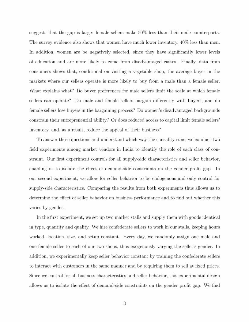
Table 9 presents the performance results for male and female sellers. Women make an

average of Rs. 175 in profits, against Rs 168 for men, a difference that is not statistically

significant (p=0.42). In terms of revenues, there are also no statistically significant differences

between men and women. On average, women earned Rs. 598, against Rs. 596 for men.

Although the difference is not statistically significant, it is striking that, on average, women

have higher profits and revenues. Since male- and female-owned businesses are equally

profitable in this experiment, we can conclude that seller behavior and buyer discrimination

24

are not first-order determinants of the gender profit gap in this context.


Next, we examine whether men and women price and bargain differently. Our data

collection protocols enabled us to assemble a rich dataset containing prices quoted and paid

for every single transaction. We test whether male and female sellers offered and charged

different prices on average. Our results show that sellers charged similar prices, regardless

of gender. Table 10 shows the prices quoted by sellers for each of the four vegetables that

we sold in our experiment. Prices are reported in Rupees per kg and correspond to the first

quote the seller gave to a prospective buyer. For all vegetables, we find no differences in prices

quotes between male and female sellers. Table 11 is analogous to Table 10, but reports final

purchase prices after any bargaining has occurred. Since our surveyors could only capture

the total transaction amounts, we restrict the sample to one-vegetable transactions. These

account for 80% of all transactions. Similarly, we find no gender differences in final prices.

Given that male and female perform equally well in this experiment, it is not surprising that

they employ similar pricing and bargaining strategies.



Finally, we turn to buyer behavior. We see a small but insignificant difference by gender

in the number of buyers who approach the seller to ask for a quote (Table 12). Women

receive 48 requests for a quote, against 44 for men, but the p-value is 0.15. Similarly, we see

a small but insignificant difference in the number of sales between men and women: women

completed 34.4 daily sales, against 31.8 for men (Table 12).


25

In Experiment 2, using a sample of real experienced sellers, we show that when exper-

imentally controlling for business characteristics, the gender of the seller does not affect

business performance. Combined with the results from Experiment 1, this rules out both

demand-side constraints and seller behavior as determinants of the gender profit gap. Even

when female and male sellers behave in a free, unscripted way, men and women perform the

same, if they are given the opportunity to run the same business.

5 Discussion

5.1 Accounting for selection in Experiment 2

In Experiment 2, we offered every seller in our baseline survey the opportunity to participate

in the experiment. Due to budget limitations, our experimental shops had to be small in

size, and therefore we did not expect all sellers to participate. Take-up was 54% for female

sellers and 48% for male sellers.

One might worry about selection into our experiment. As expected, our experiment did

not attract the top performers, since the male and female sellers we recruited are among those

who earn the least – but this was the case for both men and women. As a consequence, the

average performance in our experimental sample was slightly lower than for the representative

sample. We are able to document the extent of this selection, since among the participants

in our experiment, men report earning 35% more than women (p<0.001, Table 2). Among

our experimental pool, the gender gap in earnings is lower than in the whole population, but

still substantial. Selection only threatens the internal validity of our results if there is gender

differential selection into the experiment, that is, if male and female sellers who participate

differ along unobservable characteristics that also affect performance. Given our results, we

could be concerned that more low-performing men chose to participate.

To test the extent to which this might play a role, we first restrict our results to partici-

pants who made less than a certain threshold. Among the male sellers who participated in

26

our experiment, the highest-performing seller reported making Rs 801 per day. A natural

threshold is therefore Rs 801. After restricting our sample to male and female sellers who, in

our baseline survey, made less than Rs 801, our results are unchanged. Appendix Table 14

shows that women’s profits are on average Rs 6 higher than men’s, a very small difference

that is not statistically significant.

To further assess the role of selection, we re-estimate our results using inverse probability

weighting. We account for selection into the experiment using a logit model, and estimate

standard errors using the Generalized Method of Moments (GMM). While Table 13 shows

that being male leads to slightly higher profits, the magnitudes are very low and the co-

efficients are not statistically significant. After accounting for selection, we find no gender

profit gap, which again suggests that selection is not driving our results.


5.2 What explains the gender profit gap?

Having ruled out two potential constraints to the profitability of female-run businesses –

buyer discrimination and gender differences in bargaining and pricing – a natural question

arises: what drives the gender profit gap? In both of our experiments, women make as much

as men. What our experiments have in common is that we control for all supply-side inputs:

once women are given the same business as men, they perform equally well. Hence, one or a

combination of these supply-side inputs must explain the gap. The business characteristics

that we hold constant in both experiments are hours worked, input costs, location, inventory

composition, and inventory quantity. In what follows, we successively review each of these

business inputs and discuss which is likely to drive the observed gender disparities.

First, our survey data documents no statistically significant difference between the hours

worked by men and women (see Table 4). If anything, women report working 21 more

minutes on average (0.35 hours). Furthermore, our data captures opening and closing times

27

for each business owner’s shop, and we find no gender differences in either times. Thus, it

seems very unlikely that hours worked play a role in explaining the gender profit gap in this

context.

Second, female sellers might face higher costs, particularly at the wholesale market. This

could be due to discrimination from the vegetable traders who operate there, or because they

do not bargain as successfully as their male counterparts. We find no evidence that this is the

case. Our baseline survey elicits the price (in Rs/kg) at which vendors purchased vegetables

at the wholesale market. Across 38 of the 43 vegetables for which we have cost data for

men and women, we find no evidence that women pay a higher price. For the 5 vegetables

for which the differences in cost are statistically significant at the 10% level, the sample size

is small (ranging from 4 to 46 observations), so it is difficult to conclude that women are

at a disadvantage. Our claim is supported by anecdotal evidence and our observations at

the wholesale market. First, transactions between wholesale traders and vegetable vendors

are public and observable, which would allow all vendors to learn the day’s going rate and

compare prices across traders. Second, we observed such transactions ourselves and all

prices quoted by a given wholesale trader were the same. Third, our observations were

corroborated by the qualitative interviews we conducted with the wholesale traders. Thus,

it appears unlikely that women’s inventory costs are higher.

Third, it is possible that female sellers’ location is disadvantageous. While we cannot

completely rule this out, we think this is unlikely for two reasons. First, while walking

around the vegetable markets, we did not observe differences between the locations of male

and female shops. If location puts women at a disadvantage, it is not immediately obvious.

Second, our baseline survey documents that women’s shops receive more prospective clients

than men’s. If women’s shops are located in worse areas of the market, this constraint is not

so severe as to prevent them from attracting more prospective buyers than men.

Fourth, women may not be purchasing the right type of inventory. Since women sell on

average 7.6 different kinds of vegetables compared to men’s 6.1 (p<0.01), one would have to

28

argue that women buy too many different types of vegetables and would make more profit

by specializing in some vegetables. We find little evidence that men and women specialize

in different kinds of produce. One exception is that some men tend to specialize in onions

and sell these in very large quantities; however, women also sell onions, albeit in smaller

quantities. Excluding male sellers who specialize in onions does not change our baseline

results; the gender revenue gap is still large and significant (results not shown). Another

exception is that women tend to specialize more in chilies; however, excluding chili sellers

again yields similar results. Thus, it does not appear that inventory composition is driving

the gender gap.

Finally, we consider the quantity of inventory. There are significant gender differences in

the amount of vegetables purchased by sellers at the wholesale market; women’s inventory is

40% lower in value than men’s (Table 4). We argue that gender differences in access to capital

likely explain the gender profit gap. Indeed, women in our sample have fewer sources of credit:

among sellers who borrow money to purchase inventory, 89% of women report borrowing from

only once source (typically, family), whereas 77% of men report borrowing from two sources

(typically, family and moneylenders). Since women in this context disproportionately come

from disadvantaged backgrounds, the cost of capital is likely higher for them. Additionally,

recent research has shown that even when capital is provided to women for free, it is often

diverted to other uses, particularly towards their husbands’ businesses (Bernhardt et al.,

2019). Whether this is optimal remains an open question. By studying the productivity

of plots farmed by men and women in the same household, Udry (1996) finds evidence

of inefficient allocation of factors within the household, with women’s plots being farmed

much less intensely. Similarly, it is possible that the intra-household allocation of capital is

inefficient. More research into the capital constraints women face, with specific regard to

intra-household dynamics, is necessary to shed light on this.

While lower inventory seems to be the most likely driver of the gender profit gap, it is

possible that factors other than access to capital constrain women’s investment in inventory.

29

For example, women may not purchase as much inventory due to differences in ability, risk-

aversion, or ambition. While distinguishing these drivers is beyond the scope of this paper,

it is worth stressing that differences in access to capital would only exacerbate the effects

of such factors. If one believes that entrepreneurship is a skill that can be learned, at least

partly, lower access to capital would prevent women from ever managing larger inventory,

thus also preventing them from learning from such experiences. More research into these

factors is necessary to determine what drives women’s lower investment in inventory.

6 Conclusion

Overall, our findings show no difference in performance outcome when female and male

business owners face the same structural constraints, ruling out buyers’ discrimination and

differential seller behavior. By breaking the traditional connection between a seller’s gender

and business characteristics, our experimental design allows us to illuminate the importance

of differential business characteristics as a source of inequality for business performance.

Our two field experiments among small business owners in Jaipur mark an important

departure from prior work because they experimentally controlled for gendered differences

in business characteristics. Prior work on gender discrimination in the marketplace was not

able to distinguish whether buyers behave differently because of the seller’s gender or because

of differential business characteristics by gender. In other words, once structural constraints

are removed, buyers are indifferent to the seller’s gender.

In addition, our experimental approach enables us not only to address the role of buy-

ers’ discrimination on the gender profit gap, but also to observe the whole spectrum of

interactions between sellers and buyers–beyond looking simply at a sale or a callback. Our

methodology allows us to discern whether male and female sellers price and bargain dif-

ferently. Contrary to the results from the behavioral literature on gender differences in

negotiation, we find no difference between the way men and women bargain in this context.

30

Since we rule out demand-side constraints and seller behavior as potential determinants of

the gender profit gap, our results highlight the importance of supply-side constraints. Indeed,

in both experiments, when provided with the same business as men, women perform at least

as well, if not better. One policy implication is that policymakers and other practitioners

may want to renew efforts to provide female entrepreneurs with equal business inputs and

opportunities. While the seminal experimental studies by De Mel, McKenzie and Woodruff

(2008), De Mel, McKenzie and Woodruff (2009b) and Fafchamps et al. (2014) find zero

returns to capital for female-owned enterprises, new research by Bernhardt et al. (2019)

suggests that, in these experiments, the capital that women received was in fact re-invested

into their husbands’ businesses. This implies that the returns to capital for female-run

businesses are not necessarily zero, as previously estimated. Rather, this research highlights

the importance of family financing and intra-household allocation of resources – providing

women with access to inputs is not enough for them to use it. In light of this new study, our

experiments can be seen as a form of “extreme capital drop" intervention, since we provide

capital that is non-transferable in the form of a fully-formed business. Since we find no

gender profit gap in both experiments, our results are consistent with positive returns to

capital for both men and women. However, our shops are small in scale and our experiments

held many supply-side inputs constant, rendering it difficult to determine which of these

inputs is the driver of the gender profit gap. We see this as a promising avenue for future

research.

Finally, a distinguishing feature of our research is our precise measurement of profits

and revenues. While most of the literature on microenterprise profits relies on self-reported

measures, we measure revenue directly and precisely by counting cash. In our experiment, we

also set costs. Our measures are performance are therefore unique in their precision. Since

self-reported measures of profits are subject to considerable measurement error (De Mel,

McKenzie andWoodruff, 2009a), it is possible that the magnitude of the gap is over-estimated

due to gender differences in self-reports. This would be the case if, for instance, men tend

31

to over-report profits, while women under-report them. We acknowledge this as a limitation

in our current study, and examine this in subsequent work.

32

ReferencesBaird, Sarah, Francisco HG Ferreira, Berk Özler and Michael Woolcock. 2013. “Relative effectiveness of

conditional and unconditional cash transfers for schooling outcomes in developing countries: a systematicreview.” Campbell systematic reviews 9(8).

Becker, Gordon M, Morris H DeGroot and Jacob Marschak. 1964. “Measuring utility by a single-responsesequential method.” Systems Research and Behavioral Science 9(3):226–232.

Bernhardt, Arielle, Erica Field, Rohini Pande and Natalia Rigol. 2019. “Household matters: Revisiting thereturns to capital among female microentrepreneurs.” American Economic Review: Insights 1(2):141–60.

Bhalotra, Sonia and Tom Cochrane. 2010. “Where have all the young girls gone? Identification of sexselection in India.” IZA Discussion Papers, No. 5381, Institute for the Study of Labor (IZA), Bonn .

Bird, Sharon R and Stephen G Sapp. 2004. “Understanding the gender gap in small business success: Urbanand rural comparisons.” Gender & Society 18(1):5–28.

Blau, Francine D and Lawrence M Kahn. 2016. The gender wage gap: Extent, trends. Technical report andexplanations. Working Paper 21913, National Bureau of Economic Research.

Business Standard. 2015. “Why TV ads alone aren’t enough for India’s mobile- first consumers KernelDescription.”.

Cameron, A Colin, Jonah B Gelbach and Douglas L Miller. 2008. “Bootstrap-based improvements forinference with clustered errors.” The Review of Economics and Statistics 90(3):414–427.

Castillo, Marco, Ragan Petrie, Maximo Torero and Lise Vesterlund. 2013. “Gender differences in bargainingoutcomes: A field experiment on discrimination.” Journal of Public Economics 99:35–48.

Cirera, Xavier and Qurum Qasim. 2014. “Supporting Growth-Oriented Women Entrepreneurs: A Review ofthe Evidence and Key Challenges.” World Bank Group, Trade & Competitiveness. Innovation, Technologyand Entrepreneurshop. Policy Note. (5):1–20.

De Mel, Suresh, David J McKenzie and Christopher Woodruff. 2009a. “Measuring microenterprise profits:Must we ask how the sausage is made?” Journal of development Economics 88(1):19–31.

De Mel, Suresh, David McKenzie and Christopher Woodruff. 2008. “Returns to capital in microenterprises:evidence from a field experiment.” The quarterly journal of Economics 123(4):1329–1372.

De Mel, Suresh, David McKenzie and Christopher Woodruff. 2009b. “Are women more credit constrained?Experimental evidence on gender and microenterprise returns.” American Economic Journal: AppliedEconomics 1(3):1–32.

Doering, Laura and Sarah Thébaud. 2017. “The effects of gendered occupational roles on men’s and women’sworkplace authority: Evidence from microfinance.” American Sociological Review 82(3):542–567.

Duflo, Esther. 2012. “Women empowerment and economic development.” Journal of Economic Literature50(4):1051–1079.

Dyson, Tim and Mick Moore. 1983. “On kinship structure, female autonomy, and demographic behavior inIndia.” Population and development review pp. 35–60.

Exley, Christine, Muriel Niederle and Lise Vesterlund. 2018. Knowing When to Ask: The Cost of Leaning-in.Working Paper 6382 Department of Economics, University of Pittsburgh.URL: https://EconPapers.repec.org/RePEc:pit:wpaper:6382

33

Fafchamps, Marcel, David McKenzie, Simon Quinn and Christopher Woodruff. 2014. “Microenterprise growthand the flypaper effect: Evidence from a randomized experiment in Ghana.” Journal of developmentEconomics 106:211–226.

Fields, Gary S. 2019. “Self-employment and poverty in developing countries.” IZA World of Labor .

Fitzpatrick, Anne. 2017. “Shopping While Female: Who Pays Higher Prices and Why?” American EconomicReview 107(5):146–49.

Hardy, Morgan and Gisella Kagy. 2018. Mind The (Profit) Gap: Why Are Female Enterprise Owners EarningLess than Men? In AEA Papers and Proceedings. Vol. 108 pp. 252–55.

Hardy, Morgan and Gisella Kagy. 2019. “It’s Getting Crowded in Here: Experimental Evidence of DemandConstraints in The Gender Profit Gap.” Working Paper .

Jayachandran, Seema. 2015. “The roots of gender inequality in developing countries.” economics 7(1):63–88.

Kalleberg, Arne L and Kevin T Leicht. 1991. “Gender and organizational performance: Determinants ofsmall business survival and success.” Academy of management journal 34(1):136–161.

Kricheli-Katz, Tamar and Tali Regev. 2016. “How many cents on the dollar? Women and men in productmarkets.” Science advances 2(2):e1500599.

List, John A. 2004. “The nature and extent of discrimination in the marketplace: Evidence from the field.”The Quarterly Journal of Economics 119(1):49–89.

Petersen, Trond and Ishak Saporta. 2004. “The opportunity structure for discrimination.” American Journalof Sociology 109(4):852–901.

The Economist. 2014. “A long way from the supermarket.”.

Udry, Christopher. 1996. “Gender, Agricultural Production, and the Theory of the Household.” Journal ofPolitical Economy 104(5):1010–1046.URL: http://www.jstor.org/stable/2138950

UNDP. 2017. “United Nations Development Programme – Human Development Data (1990-2017) KernelDescription.”.URL: http://hdr.undp.org/en/data

US Bureau of Labor Statistics, U.S. Department of Labor. 2019. “Women had higher median earnings thanmen in relatively few occupations in 2018.” Economics Daily .

World Bank. 2014. Improving Access to Finance for Women-owned Businesses in India.

World Bank. 2018. World development indicators 2018. World Bank Publications.URL: https://data.worldbank.org/indicator/

34

Table 1: Female business owners disproportionately come from disadvantaged backgrounds.

Mean Female N(F) Mean Male N (M) Diff M-F p-val

Age 42.63 113 41.08 109 -1.55 0.34Number Children 3.48 128 2.63 120 -0.84 0.00Education (years) 1.16 128 7.23 120 6.07 0.00Experience (years) 17.88 128 17.55 120 -0.33 0.83Spouse Works 0.60 121 0.25 118 -0.36 0.00General Caste 0.02 128 0.25 120 0.23 0.00OBC Caste 0.34 128 0.38 120 0.05 0.44Scheduled Caste 0.45 128 0.27 120 -0.19 0.00Scheduled Tribe 0.18 128 0.07 120 -0.10 0.01Hindu 0.98 128 0.83 120 -0.14 0.00Muslim 0.02 128 0.16 120 0.13 0.00

Notes: Observational Data among a representative sample of sellers, prior to our experiment. Column 5presents the difference between columns 1 and 3. Column 6 presents the p-value from a t-test of differenceswith robust standard errors.

35

Table 2: Before our experiment: The gender gap in earning among existing sellers

Mean Female N(F) Mean Male N (M) Diff M-F p-valPanel ARepresentative sample

Daily revenue 2,396.61 192 3,590.41 193 1,193.80 0.00Weekly revenue 14,730.21 159 21,346.81 188 6,616.60 0.00Monthly revenue 50,843.33 150 77,225.00 184 26,381.67 0.00Cash-based revenue 1,199.00 95 1,730.87 69 531.87 0.01Panel BExperiment participants only

Daily revenue 2,237.22 133 3,044.92 128 807.70 0.00Weekly revenue 14,427.68 112 19,045.53 123 4,617.85 0.00Monthly revenue 54,009.43 106 72,396.67 120 18,387.23 0.06Cash-based revenue 1,005.48 52 1,507.35 34 501.87 0.02

Notes: This table presents descriptive statistics about the gender gap in earning among a representativesample of existing sellers (Panel A) and among participants in our experiment only (Panel B).Observational Data in Rupees. Column 5 presents the difference between columns 1 and 3. Column 6presents the p-value from a t-test of differences with robust standard errors. Our final experimental sampleof 282 sellers does not overlap exactly with the sellers in our representative sample of 272 sellers. The threefirst variables are measures of self-reported revenue from our observational survey. The fourth variable,“Cash estimate of revenue” is a cash estimate of revenue for a portion of the day, that we computed bytaking the difference between the cash estimate at the beginning and at the end of the survey, that wemeasured as follows. Before we started the survey, we asked the business owner how much cash s/he had atthat time. At the end, we again asked the owner how much cash she has. All these variables go in the samedirection, showing that female business owners report earning significantly less than men. We find thesame patterns whether we look at our representative sample of business owners, or at the participants inour experiment only.

36

Table 3: Before our experiment: The gender gap in earnings among a representative sampleof sellers

(1) (2) (3)Daily Revenue (Rs) Daily Revenue (Rs) Daily Revenue (Rs)

Male 1556.1∗∗∗ 1099.2∗∗∗ 911.1∗∗∗(329.2) (272.1) (330.4)

Value of Inventory (Rs) 0.343∗∗∗ 0.333∗∗∗(0.0881) (0.104)

Age -34.82∗∗(17.09)

Education (years) 18.57(43.27)

Experience 13.46(16.54)

Scheduled Caste -585.9(671.9)

Scheduled Tribe -299.1(837.7)

OBC Caste 261.1(710.0)

Hindu 284.3(714.3)

Constant 2531.4∗∗∗ 1401.6∗∗∗ 2576.7∗∗(165.5) (302.5) (1021.3)

Observations 237 237 197Mean of Dep. Var. (Male) 4087.5 4087.5 4087.5R squared 0.0884 0.328 0.373

Notes: The unit of analysis in this table is the seller. Male is an indicator variable for the business owner’sgender being male. Sample in above regressions include all business owners in our representative sample.Sample size varies slightly across columns due to missing values for some variables. All independentvariables are taken from the observational survey. Experience refers to years of experience as vegetablesellers. Robust standard errors in parentheses ∗ ∗ ∗ p < 0.01, ∗∗ p < 0.05, ∗ p < 0.1.

37

Table 4: Before our experiment: Female-owned businesses are much smaller than male-owned businesses, yet they work a similar number of hours.

Mean Female N(F) Mean Male N (M) Diff M-F p-valValue of inventory (Rs) 3,308.37 124 4,622.74 118 1,314.37 0.01Daily cost of all veg (Rs) 3,414.77 124 4,867.96 118 1,453.19 0.01Hours worked 9.11 88 8.76 56 -0.35 0.56

Notes: Observational Data prior to our experiment. The value of inventory the total amount of inventoryat the beginning of the day, valued at the price of purchase at the wholesale market. The daily cost of allveg (Rs) is the business owner’s answer when we asked them how much they have spent at the wholesalemarket that morning. We also asked the business owners to report the self-reported hours on that day.While men have 40% more inventory than women (p<0.01), men and women report working a similarnumber of hours (p=0.56).

Table 5: Before our experiment: Buyers are more likely to purchase from male sellers.

All N F Vendors N(F) M Vendors N (M) Diff M-F p-valAll Clients 0.78 436 0.72 124 0.81 312 0.09 0.04Female Clients 0.72 250 0.66 82 0.74 168 0.09 0.16Male Clients 0.87 186 0.83 42 0.88 144 0.05 0.41

Notes: Observational Data at the transaction-level prior to our experiment. Column 7 presents thedifference between columns 3 and 5. Column 8 presents the p-value from a t-test of differences with robuststandard errors. We followed buyers with their consent in the market, as they were making purchases. Thedependent variable is 1 if the buyer made a purchase from the stall, 0 otherwise. We successively considerall buyers, only female buyers, only male buyers. Conditional on visiting a stall, buyers are more likely tobuy from a male seller (p<0.05). We do not know however, whether this is due to the seller’s gender or togendered differences in business characteristics.

Table 6: Experimental Design

Experiment 1 Experiment 2Capital (type, quantity and quality of goods) Fixed FixedLocation Fixed FixedHours worked Fixed FixedSeller behavior: Bargaining and price setting Endogeneous FixedPerceived quality of goods Endogeneous FixedBuyers’ behavior Endogeneous Endogeneous

38

Table 7: Performance Results from Experiment 1

F Vendors N(F) M Vendors N(M) Diff M-F p-val

Revenue 97.50 60 63.33 57 -34.17 0.16Revenue(Trimmed) 96.73 55 67.36 53 -29.37 0.17Total Goods Sold 6.89 61 5.21 61 -1.67 0.30Total Goods Sold (Trimmed) 6.82 56 5.51 57 -1.31 0.35Total Clients 12.52 61 8.91 58 -3.61 0.09Total Purchases 5.41 61 4.66 58 -0.75 0.49% Purchased 0.43 61 0.54 58 0.11 0.00

Notes: Experimental Data. Column 5 presents the difference between columns 1 and 3. Column 6 presentsthe p-value from a t-test of differences with robust standard errors. Women performed better than men.Female sellers earn more than men on average, but this difference is mainly due to high-performing femaleoutliers, see Figure 6. Women also do more “entrepreneurial labor” since they respond to 41% more queriesof buyers. N = 122 seller-days.

Table 8: Women perform better than men, experimentally controlling for business charac-teristics and seller’s behavior

(1) (2) (3) (4)Revenue Revenue # Goods Sold # Goods Sold

Male -34.167 -32.864∗∗ -1.672 -1.678(-1.42) (-2.16) (-1.04) (-1.66)

Observations 117 117 122 119Mean of Dep. Var. (Women) 97.50 97.50 6.89 6.89R squared 0.05 0.29 0.03 0.29Controls N Y N YP-value for the testMale=0, Wild Bootstrap 0.27 0.01 0.39 0.08

Notes: Experimental Data. Above are regressions where the outcome variable is daily revenue in rupeesfrom Experiment 1, in which we experimentally controlled for seller’s behavior and all businesscharacteristics (type, quantity and quality of inventory, as well as hours worked and location). Column 1 isthe unconditional effect of being male. Column 2 includes controls for the number of days the participanttook part in the experiment, as well as for the type of confederate seller: we had both students andsurveyors acting as confederates. Standard errors clustered at the respondent level. We also report p-valuesfor standard errors computed using the wild bootstrap technique described in Cameron, Gelbach andMiller (2008). N = 122 seller-days.

39

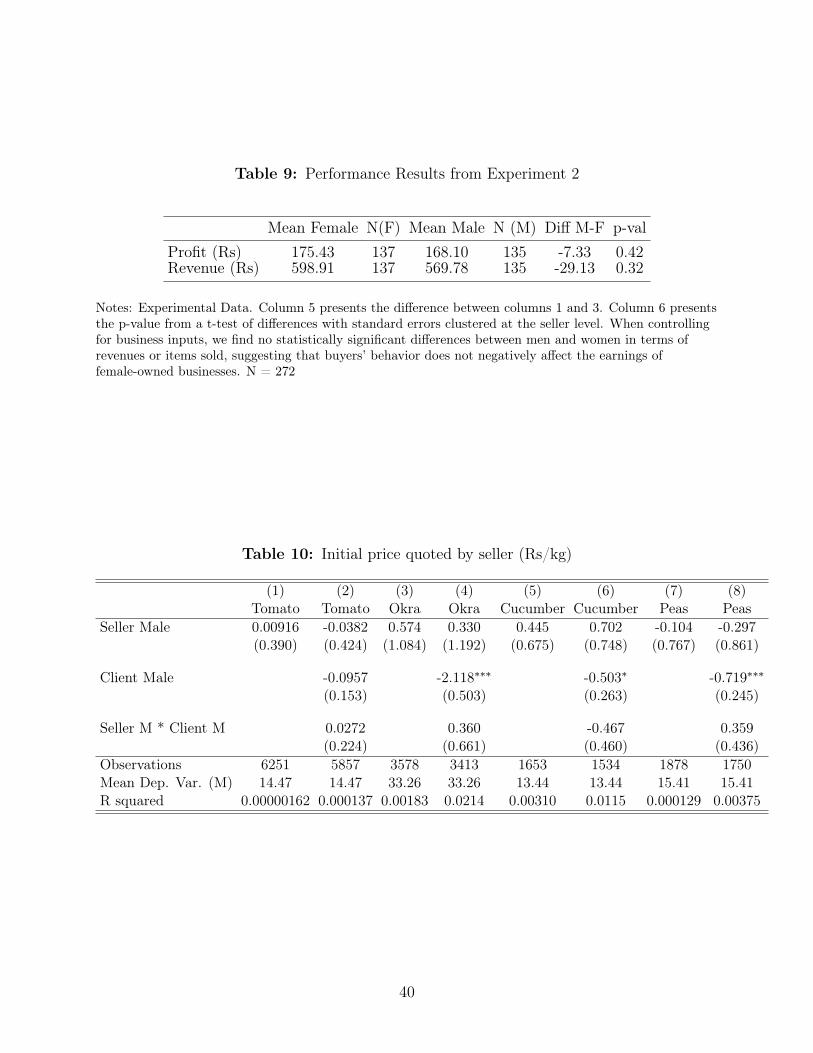
Table 9: Performance Results from Experiment 2

Mean Female N(F) Mean Male N (M) Diff M-F p-valProfit (Rs) 175.43 137 168.10 135 -7.33 0.42Revenue (Rs) 598.91 137 569.78 135 -29.13 0.32

Notes: Experimental Data. Column 5 presents the difference between columns 1 and 3. Column 6 presentsthe p-value from a t-test of differences with standard errors clustered at the seller level. When controllingfor business inputs, we find no statistically significant differences between men and women in terms ofrevenues or items sold, suggesting that buyers’ behavior does not negatively affect the earnings offemale-owned businesses. N = 272

Table 10: Initial price quoted by seller (Rs/kg)

(1) (2) (3) (4) (5) (6) (7) (8)Tomato Tomato Okra Okra Cucumber Cucumber Peas Peas

Seller Male 0.00916 -0.0382 0.574 0.330 0.445 0.702 -0.104 -0.297(0.390) (0.424) (1.084) (1.192) (0.675) (0.748) (0.767) (0.861)

Client Male -0.0957 -2.118∗∗∗ -0.503∗ -0.719∗∗∗

(0.153) (0.503) (0.263) (0.245)

Seller M * Client M 0.0272 0.360 -0.467 0.359(0.224) (0.661) (0.460) (0.436)

Observations 6251 5857 3578 3413 1653 1534 1878 1750Mean Dep. Var. (M) 14.47 14.47 33.26 33.26 13.44 13.44 15.41 15.41R squared 0.00000162 0.000137 0.00183 0.0214 0.00310 0.0115 0.000129 0.00375

40

Table 11: Final price paid by the client (Rs/kg)

(1) (2) (3) (4) (5) (6) (7) (8)Tomato Tomato Okra Okra Cucumber Cucumber Peas Peas

Seller Male 0.0196 -0.0507 0.382 1.058 -0.0328 -0.232 -0.463 -0.650(0.386) (0.430) (1.141) (1.364) (0.632) (0.726) (0.739) (0.898)

Client Male -0.0840 -1.613∗∗ -0.463 -0.462(0.203) (0.637) (0.329) (0.398)

Seller M * Client M 0.0703 -1.124 0.188 0.302(0.275) (0.976) (0.529) (0.604)

Observations 3487 3256 1497 1427 856 794 1050 986Mean Dep. Var. (M) 13.49 13.49 30.73 30.73 12.40 12.40 13.88 13.88R squared 0.00000745 0.0000676 0.000860 0.0261 0.0000182 0.00291 0.00286 0.00449

Table 12: Number of visits and sales (Experiment 2)

Mean Vendor F N(F) Mean Vendor M N (M) Diff M-F p-val

Total # visits 47.61 127 43.82 128 -3.79 0.15# female visits 19.91 127 17.14 128 -2.76 0.02# male visits 30.49 127 29.19 128 -1.30 0.56Total # sales 34.48 127 31.80 128 -2.68 0.13For F clients 11.97 127 10.31 128 -1.66 0.03For M clients 20.42 127 19.29 128 -1.13 0.39Ratio visits/sales 0.76 127 0.76 128 0.00 0.94For F clients 0.61 127 0.64 127 0.02 0.40For M clients 0.70 127 0.70 128 0.00 0.86

Notes: Experimental Data. Column 5 presents the difference between columns 1 and 3. Column 6 presentsthe p-value from a t-test of differences with robust standard errors. The unit of analysis is a seller. Numberof sales is the number of transactions for which a buyer came to the business and purchased products. Onesale is the purchase of one or more vegetables. We define a visit as any instance where a buyer asked theseller for the price of a product, whether they subsequently made a purchase or not. N = 255

41

Table 13: Results are robust to selection: Inverse probability weighting and propensityscore estimation

Selection Profit Selection Profit Selection Profit Selection ProfitMale 0.128 3.117 0.128 16.24 0.0312 7.070 0.0312 3.032

(0.68) (0.18) (0.68) (0.96) (0.17) (0.42) (0.17) (0.19)

Daily Revenue (Rs) -0.0000441 -0.0000441 -0.0111∗∗(-1.36) (-1.36) (-2.85)

Est. Profit (Survey) -0.000138 -0.000138 -0.0133(-0.77) (-0.77) (-0.70)

# Veg. for Sale -0.0136 -0.0136 -1.175 -0.0181 -0.0181 -1.958(-0.62) (-0.62) (-0.42) (-0.83) (-0.83) (-0.66)

OBC -0.228 -0.228 38.82 -0.250 -0.250 27.07(-0.78) (-0.78) (1.37) (-0.84) (-0.84) (0.91)

SC -0.0973 -0.0973 19.13 -0.0621 -0.0621 8.954(-0.32) (-0.32) (0.68) (-0.20) (-0.20) (0.30)

ST 0.00894 0.00894 10.89 0.0244 0.0244 10.95(0.02) (0.02) (0.31) (0.07) (0.07) (0.30)

Hindu 0.682 0.682 -49.50 0.742∗ 0.742∗ -37.26(1.88) (1.88) (-1.24) (1.98) (1.98) (-0.84)

Obs. (Selection) 233 233 231 231Obs. (Profit) 94 94 95 95Mean Profit (Male) 181.6 181.6 181.6 181.6t statistics in parentheses∗ p < 0.05, ∗∗ p < 0.01, ∗∗∗ p < 0.001

Notes: We use inverse probability weighting to account for selection into the experiment. Column“Selection” shows our propensity score estimation (probit). “ ‘Profit” presents the results using inverseprobability weighting. Models differ on the inclusion of controls and the use of self-reported daily revenue(“Daily Revenue”) as opposed to the estimated profit from the observational survey (“Est. Profit”) in thepropensity score equation. Overall, our results from the inverse probability weighting show that the equalperformance between men and women in Experiment 1 is not due to selection. N = 233

42

Figure 1: Our timeline for this research project.

Figure 2: A map of the 13 largest markets in Jaipur, India, that we visited for our listingsurvey

43

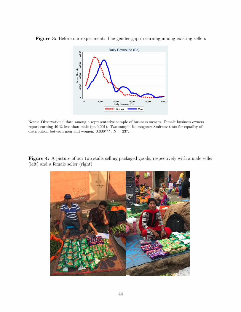
Figure 3: Before our experiment: The gender gap in earning among existing sellers

Notes: Observational data among a representative sample of business owners. Female business ownersreport earning 40 % less than male (p<0.001). Two-sample Kolmogorov-Smirnov tests for equality ofdistribution between men and women: 0.000***. N = 237.

Figure 4: A picture of our two stalls selling packaged goods, respectively with a male seller(left) and a female seller (right)

44

Figure 5: A picture of our two stalls selling vegetables, respectively with a male seller (left)and a female seller (right)

Figure 6: Results from Experiment 1: Female sellers outperformed male sellers

Notes: Experimental Data data with confederate sellers. Women perform as well, if not better. Femalesellers earn more than men on average, but this difference is mainly due to high-performing female outliers.Two-sample Kolmogorov-Smirnov tests for equality of distribution between men and women: 0.113. N =122 seller-days.

45

Figure 7: Experimental Data with confederate sellers, holding seller’s behavior constant:Women do more “entrepreneurial labor” than men

Notes: Female sellers receive more requests for information than male sellers that do not translate into apurchase. Two-sample Kolmogorov-Smirnov tests for equality of distribution between men and women:0.038**. N = 122 seller-days.

Figure 8: Results from Experiment 2: Controlling for business inputs, men and womenearn the same

Notes: When we experimentally control for business inputs, we find that women earned as much as men.Two-sample Kolmogorov-Smirnov tests for equality of distribution between men and women: 0.707. N =282

46

Appendix

A Experimentally determining the participation fee

Participants were offered a participation fee to take part in our experiment. In the first

phase of our study, we determined the amount of the participation fee for sellers through an

experimental game, to ensure that the amount was high enough to attract both men and

women. Drawing from the Becker-DeGroot-Marschak (BDM) method (Becker, DeGroot and

Marschak, 1964), our experimental game elicited the payment required by sellers to come

sell in a different market for a day, in a way that was incentive-compatible.

This procedure consisted of asking sellers how much they would be willing to receive to

sell in a different market for a day. We asked respondents in increments of Rs. 50, starting at

Rs. 200 and going up to Rs. 1000. After having elicited the minimum amount respondents

would be willing to receive as a compensation, we then drew a price at random from a

distribution of prices in increment of Rs. 50, starting from Rs. 200 and up to Rs. 1000.

If the price was above or equal to the minimum amount the respondent said they required

to sell in a different market, they were paid this amount and recruited to sell in one of our

stalls. If the price drawn was below the minimum amount they would require, they cannot

participate in our experiment.

After successful implementation of this procedure in August-September 2017, we were

confident that this game was well understood by our target population. The game was

administered to a representative subset of sellers, drawn at random within each market.

This procedure enabled us to measure a seller’s willingness to move to a different market,

which is in general not easily quantifiable. The results from this first phase showed us that

the participation fee required to take part in our experiment did not differ in a significant

manner between men and women (Figure 1). Moving forward, we decided to set the fee

at Rs 500, to ensure that enough participants, both men and women, would be willing to

come in our stalls. We therefore used this game exclusively in the first phase of our study,

48

to inform the participation fee to attract both men and women in later stages.

Figure 1: Experimentally determining that men and women require similar reservationprice to take part in our experiment

Results from our experimental game to determine the participation fee offered to sellers taking part in ourexperiment. We used the Becker-DeGroot-Marschak (BDM) method to elicit the payment required bysellers to come sell in a different market for a day, in a way that was incentive-compatible. We first askedsellers how much they would be willing to receive to sell in a different market for a day. We then drew anumber at random. Participants could only take part in our experiment if the number was below whatthey said was the minimum required to participate. This figure shows that men and women did notsignificantly differ in terms of their reservation price to take part in our experiment. N = 129

B Accounting for selection into Experiment 2

Take-up of Experiment 2 was 54% for women and 48% for men. As expected, our exper-

iment attracted the lower-performing business owners. Because of budget constraints, our

experimental stalls had to be relatively small in size; thus, expected profits could not be

high enough to attract the high-performing businesss owners. To check whether gender-

differential selection could be driving our results, we restrict our results to participants who

reported making less than Rs 801 in revenue per day in our baseline survey. This threshold

corresponds to the revenue made by the highest-performing male seller who participated in

our experiment. We refer the reader to section 5.1 for a complete discussion of selection into

the experiment.

49

Table 14: Results are robust to selection: Restricting the sample to lower performers

Mean Female N(F) Mean Male N(M) Diff M-F p-val

Daily Profit (Rs) 188.54 45 182.70 43 -5.84 0.74Daily Revenue (Rs) 921.04 45 880.86 43 -40.18 0.50

Notes: Results from Experiment 2, after restricting the sample to sellers who report revenues lower thanRs 801 in our baseline study. Our results are unchanged even among sellers who report similar levels ofbaseline earnings. This suggests a limited role for selection into the experiment.

50

does gender matter for small business performance

Documents