FACULTAD DE CIENCIAS ECONOMICAS Y EMPRESARIALES UNIVERSIDAD COMPLUTENSE DE MADRID VICEDECANATO Campus de Somosaguas, 28223 MADRID. ESPAÑA.

Documento de Trabajo 2009-007

TWO PROBLEMS OF THE TAYLOR RULE AND A PROPOSAL: THE TRACKING RULE

Alberto Alonso Jorge Uxó

FACULTAD DE CIENCIAS ECONOMICAS Y EMPRESARIALES UNIVERSIDAD COMPLUTENSE DE MADRID VICEDECANATO Campus de Somosaguas. 28223 MADRID. ESPAÑA

Esta publicación de Documentos de Trabajo pretende ser cauce de expresión y comunicación de los resultados de los proyectos de investigación que se llevan a cabo en la Facultad de Ciencias Económicas y Empresariales de la Universidad Complutense de Madrid. Los Documentos de Trabajo se distribuyen gratuitamente a las Universidades e Instituciones de Investigación que lo solicitan. No obstante, están disponibles en texto completo en el archivo institucional complutense e-prints y en el repositorio internacional de economía REPEC (http://repec.org/) con objeto de facilitar la difusión en Internet de las investigaciones producidas en este centro.

http://eprints.ucm.es/dt.html

TWO PROBLEMS OF THE TAYLOR RULE AND

A PROPOSAL: THE TRACKING RULE

Alberto Alonso

Jorge Uxó

TWO PROBLEMS OF THE TAYLOR RULE AND A PROPOSAL: THE

TRACKING RULE

Alberto Alonso and Jorge Uxó

(Universidad Complutense de Madrid)

Abstract:

This paper deals with some problems related to the application of monetary policy following

the Taylor Rule in the theoretical context of a “3-equation model”. The first problem arises if the

real interest rate does not affect the equilibrium income level itself –as in the IS curve- but its

rate of growth –as in the dynamic IS that we propose. Secondly, the Taylor Rule is incapable of

reaching the inflation target when the central bank does not correctly estimate its parameters

(the neutral interest rate and potential income) or these parameters vary. Our objective is to

propose an alternative to the Taylor Rule which overcomes both problems. This alternative has

been called the Tracking Rule, because instead of trying to estimate the neutral interest rate or

the potential output, the central bank “tracks” these values based on the economy’s evolution,

particularly on variations in the inflation and unemployment rates. After justifying the dynamic IS

and explaining the logic of this rule in detail, the paper compares the Tracking Rule with the

Taylor Rule, simulating both of them in the context of different types of shock in the modified

three equation model. The results, measured by a loss function, show that the Tracking Rule is

superior in every single case. It is particularly interesting to evaluate central bank reactions

derived from the two rules when the economy suffers a large contractive shock such as the

current crisis. The results show that, with the same shock, the economy is more likely to fall into

the liquidity trap when the Taylor Rule is applied.

Key words: Monetary Policy; Taylor Rule; Liquidity Trap; Simulations.

JEL codes: E52, E58

1. Introduction:

In the last few years, macroeconomic policies have primarily been analysed by a “three

equation model” comprising an IS equation, a Phillips curve with expectations and a monetary

policy rule, usually the Taylor Rule1.

In this theoretical context, this paper’s rationale is two-fold. Firstly, the usual IS curve is not

a satisfactory way of representing how an economy’s real sector operates in the appropriate

1 A classical presentation of this kind of models is Clarida, Galí and Gertler (1999). See also Carlin and Soskice (2006) and Galí (2008). On the other hand, Asso, Kahn and Lesson (2007) show the theoretical and applied impact of the Taylor Rule.

term for this macroeconomic policy analysis. As real economies grow at a certain rate with a

constant interest rate, it is evident that the real interest rate does not affect the equilibrium

income level itself, but its rate of growth. We have called this relationship between the

economy’s growth rate and the real interest rate the dynamic IS. Secondly, it is well known that

the Taylor Rule is incapable of reaching the inflation target when the central bank does not

correctly estimate its parameters (the neutral interest rate and potential income) or these

parameters vary2.

Considering these two problems, the Taylor Rule may well be an inappropriate guide for

central banks, so we have tried to look for and study an alternative rule. The result is the

proposed Tracking Rule, so called because instead of maintaining the estimations of the neutral

interest rate and the NAIRU constant, they are modified according to the variations registered in

the inflation rate and the level of employment.

After justifying the dynamic IS and explaining the logic of this rule in detail, the paper

compares the Tracking Rule with the Taylor Rule, simulating both of them in the context of

different types of shock in the modified three equation model. The results, measured by a loss

function, show that the Tracking Rule is superior in every single case.

It is particularly interesting to evaluate central bank reactions derived from the two rules

when the economy suffers a large contractive shock such as the current crisis. The results show

that, with the same shock, the economy is more likely to fall into the liquidity trap when the

Taylor Rule is applied. Other examples of use of the Taylor Rule for analysing both the origins

of the crisis and the appropriate monetary policy at this time, can be found in Taylor (2008,

2009). In a different theoretical context, Benhabib, Schmitt-Grohé and Uribe (2001) already

analysed the risks of falling into a liquidity trap associated to the Taylor Rule.

The paper is organised as follows. Section 2 briefly describes the model used and section 3

justifies dynamic IS in more detail. Section 4 explains the problems associated to the Taylor

Rule and presents the Tracking Rule proposed as an alternative. The paper then presents the

simulations used to compare the two rules: section 5 simulates shocks in which the economy

does not face the possibility of falling into a liquidity trap, and section 6 simulates a contractive

demand shock which could lead to such a situation, evaluating its likelihood with each rule. The

paper ends with our main conclusions.

2. Description of the model:

2.1. Equations:

In order to analyse how the two alternative monetary policy rules work, we use a simple

economic model which is similar to the “three equation model”, but adapted to a dynamic

context in which productivity, the population and the income are growing in the long term. The

model comprises the following four equations: dynamic IS, Phillips curve, the relation between

2 Taylor (1998, page 52), Woodford (2003, pages 286-288), Reis (2003).

the level of employment and the economic rate of growth, and monetary policy rule. There is

also a social welfare function to evaluate monetary policy.

The first equation, called dynamic IS, is an expression in which the income growth rate,

not its level, depends on the real interest rate, as follows:

D

ttt brDg ε+−= −1 (1)

Where g is the GDP growth rate, D and b are two positive constants, r is the real

interest rate and D

tε is an exogenous demand shock.

The second equation is the usual expression of the Phillips curve in which P& is the

inflation rate, n the percentage of employment relative to the active population and n that

percentage when the economy is at the NAIRU. Finally, a is a positive parameter and S

tε

represents possible exogenous supply shocks:

S

tt

ttn

nnaPP ε+

−+= −1

&& (2)

The third equation relates the level of employment to the income growth rate. This

equation is necessary because the interest rate affects the growth rate, but inflation depends on

the level of employment. Denoting the income level as Y , labour productivity as A and the

active population as L , we have:

tt

t

tLA

Yn =

If we assume that productivity and the active population grow, respectively, at rates γ

and l , we obtain the following equation in differences:

( )[ ]lgnn ttt +−+= − γ11

(3)

The fourth equation is one of the following two monetary policy rules:

� The first is the Taylor Rule which, in terms of the real interest rate, would be3:

3 The original Taylor Rule is expressed in terms of the output gap, but it is equivalent to the employment gap.

( )

−+−+=

n

nnPPrr tT

tt 5.05.0 && (4a)

where r is the reference interest rate used by the central bank and TP& is the inflation

target.

� The second is the Tracking Rule, and its primary characteristic is that the central bank

modifies the interest rate set in the previous period according to the changes occurring in

the level of employment, the inflation rate, and the difference between the latter and the

target rate:

( ) ( )132

1

1

11 −

−

−− −+−+

−+= tt

T

t

t

tttt PPPP

n

nnrr &&&& ααα (4b)

1α ,

2α and

3α are positive parameters.

The primary objective of this paper is to analyse the economy’s dynamic performance

under different shocks with each of these two rules.

2.2. Welfare function and shocks:

The welfare function is a quadratic loss function which depends on inflation deviations

from target and the output gap, where δ is the discount factor and P&

λ and OGλ represent the

weightings of the inflation and income targets:

( )[ ]∑=

+−=T

t

tOG

T

ttP

t OGPPPS0

22

λλδ &&& (5)

Possible economic shocks are divided according to two main criteria. Taking into

account the shock’s origin, we distinguish between shocks affecting the growth rate of

aggregate demand, inflationist shocks, a structural change affecting the NAIRU value and a

change in the productivity or active population growth rates.

Depending on the shock’s duration, a first group would comprise transitory shocks,

represented through an autoregressive process. For example, for a demand shock it would be:

D

t

D

t 1* −= ερε , where 10 << ρ . A second group would include permanent shocks, in which

the changes in one of the model’s exogenous variables are so long-lasting that 1=ρ .

2.3. Equilibrium position:

For the model to be at equilibrium, the four endogenous variables (the growth rate, the

inflation rate, the employment level and the interest rate) must remain stable. This only occurs

in the following conditions:

� When the employment level is as corresponds to the NAIRU; otherwise, the inflation rate

will vary.

� The growth rate must be equal to the sum of the productivity and active population growth

rates; otherwise, the level of employment will not remain constant. This sum is called

“potential growth rate” ( )g :

lg += γ (6)

� For the above condition to be met, the interest rate must be such that, according to the IS,

the growth rate is at its potential value. This equilibrium interest rate is called “neutral

interest rate” ( )r :

b

gDr

−= (7)

If these three conditions are met, the inflation will remain stable, albeit at any value. The

economy, therefore, can reach equilibrium even though inflation is not at the rate targetted by

the central bank.

3. Justification of dynamic IS:

The intuition underlying the idea of a dynamic IS is that the natural status of an economy in

which part of the income is saved is to growth at a certain rate, and that changes in the interest

rate affect that growth rate and not the equilibrium income level. We will try to express this idea

and to compare it with an alternative formulation.

1. The most simple way of writing the IS equation is:

tt braY −= (8)

Where Y is the equilibrium income value at the end of the multiplier process. We

call this equation the “static IS”.

For this formulation to show the growth undergone by real economies, there would

have to be continuous drops in the real interest rate. Then, in order to adapt this

formulation to a growing economy, we can suppose that potential GDP ( )POT

tY

grows at an exogenous trend ( )θ and that the interest rate affects –with a lag- the

output gap. We could write this “IS with trend” as:

1−−=−

= tPOT

t

POT

ttt bra

Y

YYOG (9)

Once we consider the trend, we obtain the potential income at period t, as follow:

( )tPOTPOT

t YY θ+= 10

(10)

And the final expression of the IS would be:

( )1

1 −−+= t

POT

tt braYY (11)

Or:

( ) ( )10

11 −−++= t

tPOT

t braYY θ (12)

This formulation, however, does not well resolve the problem of going from a static

idea of the economy to another with continuous growth. According to expression

(12), if the interest rate rises during a few periods, the GDP would be beneath its

potential level by a constant percentage. Moreover, the interest rate would only

have to return to that value for the output gap to be zero. The period of contraction

would have made no mark on the economy. In a dynamic economy, however, this

process would probably be more complex: for the output gap to close, the economy

would have to grow at more than its potential rate for a few periods (the trend, in

this formulation), which in turn would require a lower than neutral interest rate.

2. In the dynamic IS, all expenditure items must depend on income. More specifically,

for each interest rate, consumption and investment demand values are proportional

to the period’s income. In other words, in an economy in which income has doubled,

the number of cost-effective investment projects for a given interest rate will also

have doubled, and the same will have occurred to consumption demand. It has to

be assumed, therefore, that economic growth does not alter the consumption/saving

preference ratio or the viability of investment projects (in proportion to income) for

each interest rate.

For the formulation to be dynamic – in Hicks’ terminology, for the period’s

explanation not to be self-contained – there must be a lag in the mutual

dependence of income and expenditure. There are two ways in which this can be

formalised. Firstly, this lag could be because the investment and consumption

decisions in a period are made by individuals according to the previous period’s

income, known as the Robertson lag. Denoting total aggregate demand with DA , a

schematic formulation would be:

tt DAY = (13a)

ttt ICDA += (14a)

t

t

t rcCY

C−=

−1

(15a)

t

t

t redY

I−=

−1

(16a)

Alternatively, however, it could be assumed that the production of period t is

generated with a delay relative to the demand decided in t-1, which will depend on

the income obtained in t-1 – Lundberg lag-. This gives us:

1−= tt DAY (13b)

111 −−− += ttt ICDA (14b)

1

1

1

−

−

− −= t

t

t rcCY

C (15b)

1

1

1

−

−

− −= t

t

t redY

I (16b)

We prefer the second possibility, because it considers the delay between the real

interest rate and the economic growth rate which we find in real economies4.

Indeed, from equations (13b) to (16b), we obtain:

( )1

1

−

−

+−+= t

t

t recdCY

Y (17)

With 1−+= dCD and ( )ecb += , we obtain the expression of dynamic IS:

4 Ball (1997) uses a similar equation, also called dynamic IS, and he also mentions this lag.

1−−= tt brDg (1)

3. This expression is significantly different from the IS in (12). In this expression, we

can see that direct determination of the output gap according to the period’s interest

rate is “superimposed” on the long-term exogenous trend. However, in a dynamic

IS, the interest rate determines the rate of growth, and the output gap evolves

according to the difference between the real and potential growth rates. We can see

this in the following expression of a period’s income from (1):

( )11

1 −− −+= ttt brDYY (18)

If we assume that income is at its potential level in the initial period, from when

there is a constant interest rate, we have the following expression of income at

period t:

( )tPOT

t brDYY −+= 10

(19)

If the interest rate is neutral in the dynamic IS, the economy grows at its potential

rate and, with a zero output gap, income will also be at its potential value in all

periods. If the interest rate is higher than the neutral rate, however, the economy will

grow at less than its potential rate and there will be a growing negative output gap.

The difference lies in the fact that when the interest rate moves away from the

“neutral” rate in (12)5, there is also an output gap, but it remains constant over time.

Furthermore, in order to eliminate the output gap with the dynamic IS, the interest

rate would have to be below the neutral level for a time, while it would only have to

return to its neutral level with expression (12).

Another difference is found when comparing expressions (18) and (11). In the

proposed dynamic IS, the interest rate has an impact on the relationship between a

period’s income and the previous period’s effective income – which has an impact

on consumer and investment decisions (aggregate demand). In the usual IS,

however, Say’s Law appears to be applicable, as the reference is always to

potential income rather than the economy’s actual income.

In our opinion, this more complex description of the economy’s evolution when the

interest rate varies is also more realistic. Therefore, the use of dynamic IS is particularly

important because it enables us to explore the difficulties involved in regulating an economy in

5 The interest rate with which the output gap is zero. In this case: b

ar = .

which the interest rate affects the growth rate but inflation rate variations depend on the

difference between effective and potential income levels.

4. The problems of the Taylor Rule and a proposed solution:

4.1. Theoretical problems of the Taylor Rule:

The logic of the Taylor Rule is that the central bank uses a reference interest rate which

is established providing that the inflation rate is on target and the economy registers its potential

income level. It would be reasonable to believe, therefore, that this reference interest rate will be

such that this situation is maintained over time (neutral interest rate). When this condition is not

met, the authorities change the nominal interest rate in an attempt to obtain a real rate which is

higher or lower than the neutral rate, depending on the problem to be solved.

Is such a rule an appropriate guide for monetary policy? In our opinion, it is not,

because of two problems associated to the Taylor Rule.

The first problem arises if the model used by the authorities does not include a dynamic

IS, because the neutral interest rate they will attempt to estimate to be used as a reference for

monetary policy will not be appropriate. Indeed, the central bank will estimate an interest rate

such that the economy will register potential income in the medium term6, when it should – with

a dynamic IS – estimate the rate that will maintain the economy at potential growth.

Furthermore, the terms of the rule only include the income level, but not the growth rate.

This means that monetary policy will react the same to a given output gap, irrespective of the

economic growth rate. Assuming a negative output gap, the central bank should, however,

apply a more expansionary monetary policy if the economy is registering a low growth rate than

if the economy is growing at a high rate. In the first case, the economy’s cyclical status would be

worsening, whereas in the second it would be undergoing a correction process.

The second problem facing the authorities when attempting to apply a Taylor-like rule is

that they cannot observe the two reference values for the application of monetary policy – the

neutral interest rate and the equilibrium employment level – so they have to estimate their most

likely values. This estimation, however, is subject to some uncertainty7, so errors can lead to

unsatisfactory results.

Orphanides y Williams (2002) believe that the uncertainty regarding the estimation of

these two variables could be due to not knowing which is the true theoretical model, to the level

of information available in real-time (when interest rate decisions are made), and to the 6 This definition is the same as used by Greenspan (1993), Blinder (1998, page 32) and Woodford (2003, page 248). 7 The difficulty involved in estimating these two variables is empirically documented. For the monetary union, for instance, Crespo Cuaresma, Gnan and Ritzberger-Grünwald (2005) present a broad summary of the estimates of the neutral interest rate obtained by different procedures and the large differences found in the results obtained. Benati and Vitale (2007) estimate both the neutral interest rate and the NAIRU, showing that they are both subject to a high degree of variability over time and that their estimated value is affected by significant uncertainty. Similar conclusions are reached for the United States by Wu (2005).

existence of different estimation methods. The problem is actually greater: even if the central

bank has been able to correctly estimate these two variables in a given period, any economic

shock would alter at least one of the two values. As a result, the central bank would be

attempting to compensate for the effects of a shock with a rule based on a reference which the

same shock has changed.

Assume, for instance, a negative demand shock which moves the IS downwards. If the

central bank wishes to compensate for this drop in the aggregate demand growth rate, so that

the economy can continue to grow at its potential rate, it will have to establish a lower interest

rate. This is the only way to stimulate the growth rate enough while the unemployment rate

remains constant. The neutral interest rate will therefore have changed.

If this shock is transitory, for instance lasting for only one period, the neutral interest rate

will rapidly return to its initial value and the error associated to the Taylor Rule will not be very

significant, especially if we consider the delay with which monetary policy is effective. These

one-period shocks, however, are not the most important from a monetary policy perspective,

and changes in aggregate demand are more likely to disappear gradually, if they do so at all.

The variation in the neutral interest rate will last longer, then, and the costs derived from

incorrectly estimating the equilibrium interest rate will increase as shocks persist.

Likewise, any shock on the supply side will affect the equilibrium values that the central

bank is using as a reference for application of its monetary policy. Consider an inflationist

shock ( )0>S

tε . To maintain inflation constant will require a higher unemployment rate; the

NAIRU will therefore change and this is not considered by the Taylor Rule. As before, if the

shock lasts for a single period, the cost of this will be insignificant, but it will tend to grow as the

supply shock persists. Another example could be a structural change in how the labour or

goods markets operate. In this case, the NAIRU would be permanently changed.

The following section provides a detailed analysis of the problems derived from these

estimation errors.

4.2. Consequences of an error in the estimation of the neutral interest rate or the NAIRU:

An error when estimating these reference values creates two types of problem: the

inflation rate that characterises the economy’s equilibrium could be other than the target rate,

and the adjustment process towards this equilibrium could be too slow and costly or give rise to

an unstable dynamic process.

This can be seen by assuming first that there is a permanent shock and analysing the

economy’s equilibrium (if reached). We then consider the consequences of this error for the

dynamic adjustment process and the case of a transitory shock.

Using BCr to denote the “neutral” interest rate estimated by the central bank and BCn

to denote the employment level that the central bank believes is compatible with stable inflation,

the Taylor Rule would be as follows:

( )

−+−+=

BC

BC

tT

t

BC

tn

nnPPrr 5.05.0 && (20)

Earlier, we saw that equilibrium would be characterised by a constant interest rate and a

constant employment level, that is rr = and nn = ; if these two conditions are substituted in

the monetary policy rule:

( )

−+−+=

BC

BCTBC

n

nnPPrr 5.05.0 && (21)

This expression shows that, whenever there is an error in the estimation of the interest

rate or the employment level associated to the NAIRU by a central bank which applies its

monetary policy according to the Taylor Rule, the economy will stabilise at an inflation rate ( )P&

which differs from the target rate. This “inflationist bias” will be equal to:

( )

5.0

5.0

−−−

=−BC

BCBC

T n

nnrr

PP && (22)

So inflation will be higher than the target rate whenever the central bank estimates a too

low neutral interest rate or NAIRU.

The problem could be even greater, however, if the error is in an upwards direction and

the central bank has also established a low inflation target; in this case, the equilibrium inflation

rate could be negative or could even require a negative nominal interest rate to reach the real

neutral interest rate. The economy would then face the problem of the liquidity trap. Specifically,

the nominal interest rate that the central bank should establish at equilibrium ( )i would be:

( )

5.0

5.0

−−−

++=+=BC

BCBC

T n

nnrr

PrPri && (23)

Is there a high risk of this rate being negative? It can certainly not be ruled out. If the

estimated real neutral interest rate is 2% and the inflation target is also 2%, the real neutral

interest rate would only have to fall by 1.35 percentage points for the equilibrium nominal

interest rate to be negative, or it would only have to fall by one percentage point if the central

bank was overestimating the NAIRU by a bit more than one point.

We will be returning later to this possible economic instability problem. For the time

being, assume that the economy returns to a new equilibrium after the shock. It is important to

note that, besides this equilibrium being characterised by an inflation rate different than target,

the adjustment process will also be a slow one, as a result of using references which are no

longer valid.

This monetary policy maladjustment would certainly have a cost in terms of greater

inflation or employment rate deviations relative to the central bank’s targets, as shown by our

simulations.

This also shows that, although the difference between the actual and target inflation

rates would not be maintained at long-term equilibrium if the shock is not permanent (or if the

central bank corrects its reference values after a few periods), the problem could extend to any

shock which persists some time. They all affect the interest rate or equilibrium employment (or

both) for several periods, in which the Taylor Rule would be setting an interest rate that is not

the adequate for the economy’s circumstances.

4.3. An alternative monetary policy rule:

What type of rule could prevent these two problems? The alternative proposed here is a

modification of the Taylor Rule characterised by two principal ideas.

� First, the concept of neutral interest rate that the central bank uses as a reference for its

monetary policy is derived from a dynamic IS.

� Secondly, the central bank does not estimate this neutral interest rate or the NAIRU.

Instead of this, the rule “tracks” these values based on the economy’s evolution, particularly

on variations in the inflation and unemployment rates.

This Tracking Rule is formally derived from the original Taylor Rule:

( )

−+−+=

n

nnPPrr tT

tt 5.05.0 && (4a)

The two terms which are unknown to the central bank are the neutral interest rate and

the difference between the effective employment rate and that associated to the NAIRU. How

can they be identified with the information available?

If the interest rate applied in the previous period was the neutral rate, the growth rate

will be at its potential value and the employment rate will remain the same. On the other hand, a

discrepancy between the actual interest rate and the neutral rate will lead to a change in

employment, so this variation can be used to know the difference between the current and the

neutral interest rate.

Specifically, according to the IS, the period’s growth rate depends on the previous

period’s real interest rate:

1−−= tt brDg

Replacing the interest rate with the neutral rate, we obtain the potential growth rate:

rbDg −=

But if these two expressions are subtracted:

b

ggrr tt

−+= −1 (24)

Finally, according to (3), the difference between the actual and the potential growth rate

is equal to the percentage variation in the employment level. Then:

1

1

1

1

−

−−

−+=

t

tt

tn

nn

brr (24b)

A similar reasoning applies to the NAIRU. If the current employment rate is indeed the

economy’s NAIRU, inflation would remain stable. However, any difference between the current

unemployment rate and the NAIRU would be reflected in a change in the inflation rate. Based

on the Phillips curve:

( )1

1−−=

−tt

t PPan

nn&& (25)

Replacing (24b) and (25) in the Taylor Rule, we obtain the Tracking Rule:

( ) ( )132

1

1

11 −

−

−− −+−+

−+= tt

T

t

t

tttt PPPP

n

nnrr &&&& ααα (4b)

Where b

11

=α , 5.02

=α and a

5.03

=α . Giving parameter b a value of 0.8 and a

value of 0.4 to parameter a 8:

( ) ( )1

1

1

125.15.025.1 −

−

−− −+−+

−+= tt

T

t

t

tttt PPPP

n

nnrr &&&& (4c)

8 These values are taken from the calibration of a three-equation model by Aarle, Garretsen and Huart (2004, table 1, page 418) for the monetary union.

As we can see, the logic of the rule would be to start with the previous period’s interest

rate and change it whenever there are signs that the economy is not at the desired equilibrium.

Specifically, the central bank should alter the previous period’s interest rate :

1. When employment is varying, as this shows that the growth rate is not at its potential value,

so the current interest rate is not the neutral rate. For example, if the unemployment rate is

rising, this means that the interest rate is higher than the neutral rate, and it should be

reduced by the central bank. With this term, it “tracks” the neutral interest rate.

2. When the rate of inflation is varying, as this shows that the unemployment rate, however

constant, is not the equilibrium rate. For example, the central bank should increase the

interest rate whenever inflation accelerates, as this shows that the unemployment rate is

lower than the NAIRU, which the central bank is “tracking” with this term of the rule.

3. When inflation is at other than target level, to prevent the economy from stabilising with a

constant, but undesired, employment and inflation rate.

As this rule does not include an estimate of the neutral interest rate or NAIRU, it is not

affected by the problem of the long-term equilibrium of the economy being characterised by

other than target inflation. Indeed, we saw earlier that, at equilibrium, rrr tt == −1 ,

nnn tt == −1 and 1−= tt PP && , and substituting in (4b), we have that:

( ) ( )1

1

1

125.15.125.1 −

−

−− −+−+

−+= tt

T

t

t

tttt PPPP

n

nnrr &&&&

0=− TPP && (26)

For the Tracking Rule to be defined as better than the Taylor Rule, we also have to

compare its ability to take the economy to equilibrium without major fluctuations. The following

sections therefore simulate different shocks, comparing the economy’s trajectory when the

authorities apply the Taylor Rule or the Tracking Rule. We can anticipate that one important

conclusion is that this rule mitigates the excessively cautious monetary policy derived from the

Taylor Rule.

It is also important to note some similarities between this rule and the generalization of

the Taylor Rule proposed by Orphanides (2007) to tackle the problem of uncertainty concerning

the real values of neutral interest rate and potencial income. This rule is as follows:

( )( ) ( ) ( ) ( )ttYtY

T

tPti

T

it YYYYPPiPri ∆−∆+−+−+++−= ∆− φφφφφ &&&&1

1

Where iφ , P&

φ , Yφ and Y∆φ are positive parameters, Y is the income and Y is the

potential income. Taylor Rule would be a particular case of this general rule, where

0== ∆Yi φφ . According to Orphanides, however, when the uncertainty about estimations of

neutral interest rate and potential income is high, we should use the values 1=iφ and

0=Yφ , so

( ) ( )ttY

T

tPtt YYPPii ∆−∆+−+= ∆− φφ &&&1

This rule is similar to the Tracking Rule as it uses the interest rate of the previous period

and not the estimation of the “neutral” interest rate. Nevertheless some important differences

can be appreciated:

� The potencial growth rate still appears in this rule, although it cannot be observed. It

is for that reason that, in our rule, the difference between real growth and potential

growth is substituted by the variation in the employment level, which, in fact, can be

observed.

� Orphanides introduces this term as an approximation for the differences between

effective income and potential income, which is more difficult to calculate. However,

this term is included in the Tracking Rule to “track” the neutral interest rate based

on the dynamic IS.

� While Orphanides removes the term of the output gap, we “track” this gap by

including the changes in inflation. Our simulations show that the stabilizing

properties of the Rule are enhanced through the inclusion of the changes in inflation

above mentioned.

5. Comparison of the two rules when there is no liquidity trap risk:

This and the following section present the results of simulations made to show the

dynamic adjustment and equilibrium reached by the economy after different shocks. It is initially

considered that the shock is permanent, but we afterwards continue by considering that the

shock follows an auto-regressive process.

We study two main cases. The first, which is approached in this section, is one in which

the economy is stable with both rules, and we will want to know the inflation deviations from

target and income deviations from its potential, both at final equilibrium and during the

adjustment process. The second case, which is found in the following section, analyses the risk

of the economy finally falling into a liquidity trap with each of the rules, after a significant drop in

demand.

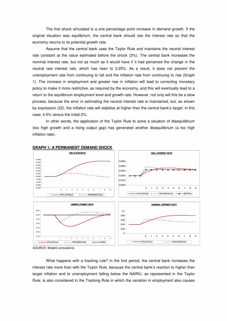
The first shock simulated is a one percentage point increase in demand growth. If the

original situation was equilibrium, the central bank should rise the interest rate so that the

economy returns to its potential growth rate.

Assume that the central bank uses the Taylor Rule and maintains the neutral interest

rate constant at the value estimated before the shock (2%). The central bank increases the

nominal interest rate, but not as much as it would have if it had perceived the change in the

neutral real interest rate, which has risen to 3.25%. As a result, it does not prevent the

unemployment rate from continuing to fall and the inflation rate from continuing to rise (Graph

1). The increase in employment and greater rise in inflation will lead to correcting monetary

policy to make it more restrictive, as required by the economy, and this will eventually lead to a

return to the equilibrium employment level and growth rate. However, not only will this be a slow

process, because the error in estimating the neutral interest rate is maintained, but, as shown

by expression (22), the inflation rate will stabilise at higher than the central bank’s target: in this

case, 4.5% versus the initial 2%.

In other words, the application of the Taylor Rule to solve a situation of disequilibrium

(too high growth and a rising output gap) has generated another disequilibrium (a too high

inflation rate).

GRAPH 1: A PERMANENT DEMAND SHOCK SOURCE: Model’s simulations.

What happens with a tracking rule? In the first period, the central bank increases the

interest rate more than with the Taylor Rule, because the central bank’s reaction to higher than

target inflation and to unemployment falling below the NAIRU, as represented in the Taylor

Rule, is also considered in the Tracking Rule in which the variation in employment also causes

INFLATION RATE

0,0000

0,0050

0,0100

0,0150

0,0200

0,0250

0,0300

0,0350

0,0400

0,0450

0,0500

0 1 2 3 4 5 6 7 8 9

TAYLOR RULE TRACKING RULE

UNEMPLOYMENT RATE

7,50%

8,00%

8,50%

9,00%

9,50%

10,00%

10,50%

0 1 2 3 4 5 6 7 8 9

TAYLOR RULE TRACKING RULE NAIRU

NOMINAL INTEREST RATE

0

0,02

0,04

0,06

0,08

0,1

0 1 2 3 4 5 6 7 8 9

TAYLOR RULE TRACKING RULE

REAL INTEREST RATE

0,0000

0,0100

0,0200

0,0300

0,0400

0,0500

0 1 2 3 4 5 6 7 8 9

TAYLOR RULE TRACKING RULE NEUTRAL

the interest rate to rise further, so the central bank is anticipating the increase in the neutral

interest rate.

This reduction is sufficient for the growth rate to fall beneath its potential value, so the

unemployment rate starts to rise. Monetary policy also adapts faster to the restrictive tone

required in the following periods, because its reference is not a fixed interest rate, but the

previous period’s interest rate, which is rising. As we see in Graph 1, this does not only prevent

inflation from rising earlier, but also ensures that the economy returns to its original equilibrium.

Finally, the question is how these two monetary policy rules compare if the shock is not

permanent. As is to be expected, the cost of using the Taylor Rule is smaller when the

persistence of shocks is smaller, for two reasons. First, because the inflationist bias created at

equilibrium (expression (22)) disappears. Secondly, because the shorter the shock, the shorter

is the duration of the central bank’s error in the references used for its monetary policy.

However, as shown on Graph 2 and Table 1, this cost does not vanish completely, as the rise in

the growth rate (above the potential level) and inflation (above target) and the reduction in the

unemployment rate (beneath equilibrium) is greater than with the Tracking Rule.

GRAPH 2: TRANSITORY DEMAND SHOCK (ρ=0,75) SOURCE: Model’s simulations.

TABLE 1: SOCIAL WELFARE LOSS AFTER A DEMAND SHOCK (+1p.p.)*

Persistence (ρ) Taylor Rule Tracking Rule1 0.502** 0.014

0.75 0.07 0.0120.5 0.0329 0.010 0.132 0.009

* Value of the social loss function (5) assuming that 5.0== OGPλλ &

.

** When the shock is permanent (ρ=1) the social loss is always rising with the Taylor Rule, because the equilibrium inflation rate is not the central bank’s target. The figure in the table is for the period in which the equilibrium is reached. SOURCE: Model’s simulations.

INFLATION RATE

0,0000

0,0050

0,0100

0,0150

0,0200

0,0250

0,0300

0,0350

0,0400

0 1 2 3 4 5 6 7 8 9

TAYLOR RULE TRACKING RULE

UNEMPLOYMENT RATE

8,00%

8,50%

9,00%

9,50%

10,00%

10,50%

11,00%

0 1 2 3 4 5 6 7 8 9

TAYLOR RULE TRACKING RULE NAIRU

NOMINAL INTEREST RATE

0

0,01

0,02

0,03

0,04

0,05

0,06

0,07

0 1 2 3 4 5 6 7 8 9

TAYLOR RULE TRACKING RULE

REAL INTEREST RATE

0,0000

0,0100

0,0200

0,0300

0,0400

0,0500

0 1 2 3 4 5 6 7 8 9

TAYLOR RULE TRACKING RULE NEUTRAL

We have also studied what would happen if shocks originate on the supply side. We

specifically simulated a 2-percentage point increase in the NAIRU which was not anticipated by

the central bank. As a result of the shock, the initial effect will be an increase in inflation to

2.8%, and if the central bank applies the Taylor Rule, both the nominal and real interest rates

will increase. Specifically, the nominal interest rate would go from 4% to 5.2% and the real

interest rate would be 2.4%.

This central bank reaction is a move in the right direction and will cause an increase in

the employment rate, which is required in order to stabilise inflation. Inflation, however, will

continue to grow, because this new unemployment rate is still below the economy’s new

NAIRU, although it is above the NAIRU estimated by the central bank. This is very important,

because even though monetary policy should continue to be restrictive, by calculating the

Taylor Rule with the wrong NAIRU (too low), the nominal interest rate will rise less than it

should. Inflation will continue to accelerate and, when the economy returns to the neutral

interest rate, it will stabilise at higher than the initial rate of inflation (4.3%), as shown on Graph

3, because the unemployment rate is lower than the NAIRU during nearly the entire adjustment

process.

If the Tracking Rule is applied, the same differences occur as in the case of demand

shocks: the nominal interest rate will grow faster, as the central bank will immediately react to

the fall in the NAIRU through accelerating inflation. Thanks to this more active monetary policy

reaction, inflation will start to fall earlier, so both the nominal and real interest rates would

increase more rapidly. Eventually, the economy would stabilise again at the target inflation rate.

Table 2 shows the differences in the value of the Welfare Function derived from

application of the Taylor Rule or the Tracking Rule when the supply shock has different degrees

of persistence.

GRAPH 3: A RISE IN THE NAIRU

SOURCE: Model’s simulations.

INFLATION RATE

0,0000

0,0050

0,0100

0,0150

0,0200

0,0250

0,0300

0,0350

0,0400

0,0450

0,0500

0 1 2 3 4 5 6 7 8 9

TAYLOR RULE TRACKING RULE

UNEMPLOYMENT RATE

0,00%

2,00%

4,00%

6,00%

8,00%

10,00%

12,00%

14,00%

0 1 2 3 4 5 6 7 8 9

TAYLOR RULE TRACKING RULE NAIRU

NOMINAL INTEREST RATE

00,010,020,030,040,050,060,070,08

0 1 2 3 4 5 6 7 8 9

TAYLOR RULE TRACKING RULE

REAL INTEREST RATE

0,0000

0,00500,0100

0,0150

0,0200

0,02500,0300

0,0350

0,0400

0 1 2 3 4 5 6 7 8 9

TAYLOR RULE TRACKING RULE NEUTRAL

TABLE 2: SOCIAL WELFARE LOSS AFTER A RISE IN THE NAIRU (+2p.p.)*

Persistence (ρ) Taylor Rule Tracking Rule1 0.477** 0.074

0.75 0.0935 0.0630.5 0.0572 0.0520 0.0376 0.044

* Value of the social loss function (5) assuming that 5.0== OGPλλ & .

** When the shock is permanent (ρ=1) the social loss is always rising with the Taylor Rule, because the equilibrium inflation rate is not the central bank’s target. The figure in the table is for the period in which the equilibrium is reached. SOURCE: Model’s simulations.

6. Monetary policy and the present crisis. The liquidity trap risk with both rules:

One of the characteristics of the present crisis is that economies are suffering a large

and persistent drop in aggregate demand. In the model, this could be seen as a permanent

contractive demand shock. We would like to see the results of the application of each of the two

rules in these circumstances and, in particular, the likelihood in each case of the economy

falling into a liquidity trap.

This analysis is performed in two complementary manners. We first simulate a fall in the

demand growth rate, to analyse the differences occurring in the economy’s dynamics depending

on the rule that is applied. This will show us why the liquidity trap risk is greater with the Taylor

Rule. We then attempt to evaluate the minimum size of demand shock required for the economy

to fall into a liquidity trap with each rule, finding that, with the Tracking Rule, this situation occurs

with shocks twice the size as with the Taylor Rule.

We therefore start by assuming that the economy is at equilibrium and that the

aggregate demand growth rate falls by one percentage point, also reducing the neutral interest

rate to 0.75%.

How would the central bank reaction in one case or the other? The nominal interest rate

will fall with both rules, but we have seen here that this reaction will be more cautious with the

Taylor Rule in the first few periods. As a result, the unemployment rate will continue to grow and

inflation will continue to fall, although it would already be recovering with the Tracking Rule.

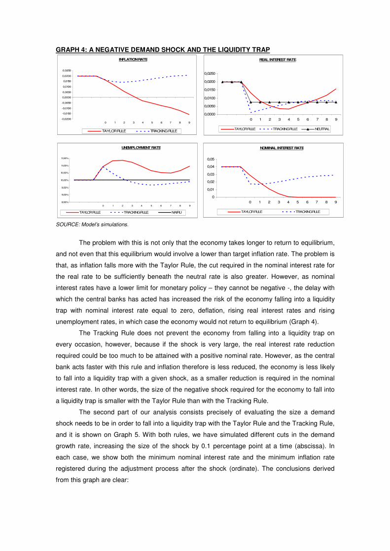
GRAPH 4: A NEGATIVE DEMAND SHOCK AND THE LIQUIDITY TRAP

SOURCE: Model’s simulations.

The problem with this is not only that the economy takes longer to return to equilibrium,

and not even that this equilibrium would involve a lower than target inflation rate. The problem is

that, as inflation falls more with the Taylor Rule, the cut required in the nominal interest rate for

the real rate to be sufficiently beneath the neutral rate is also greater. However, as nominal

interest rates have a lower limit for monetary policy – they cannot be negative -, the delay with

which the central banks has acted has increased the risk of the economy falling into a liquidity

trap with nominal interest rate equal to zero, deflation, rising real interest rates and rising

unemployment rates, in which case the economy would not return to equilibrium (Graph 4).

The Tracking Rule does not prevent the economy from falling into a liquidity trap on

every occasion, however, because if the shock is very large, the real interest rate reduction

required could be too much to be attained with a positive nominal rate. However, as the central

bank acts faster with this rule and inflation therefore is less reduced, the economy is less likely

to fall into a liquidity trap with a given shock, as a smaller reduction is required in the nominal

interest rate. In other words, the size of the negative shock required for the economy to fall into

a liquidity trap is smaller with the Taylor Rule than with the Tracking Rule.

The second part of our analysis consists precisely of evaluating the size a demand

shock needs to be in order to fall into a liquidity trap with the Taylor Rule and the Tracking Rule,

and it is shown on Graph 5. With both rules, we have simulated different cuts in the demand

growth rate, increasing the size of the shock by 0.1 percentage point at a time (abscissa). In

each case, we show both the minimum nominal interest rate and the minimum inflation rate

registered during the adjustment process after the shock (ordinate). The conclusions derived

from this graph are clear:

INFLATION RATE

-0,0200

-0,0150

-0,0100

-0,0050

0,0000

0,0050

0,0100

0,0150

0,0200

0,0250

0 1 2 3 4 5 6 7 8 9

TAYLOR RULE TRACKING RULE

UNEMPLOYMENT RATE

8,50%

9,00%

9,50%

10,00%

10,50%

11,00%

11,50%

0 1 2 3 4 5 6 7 8 9

TAYLOR RULE TRACKING RULE NAIRU

NOMINAL INTEREST RATE

0

0,01

0,02

0,03

0,04

0,05

0 1 2 3 4 5 6 7 8 9

TAYLOR RULE TRACKING RULE

REAL INTEREST RATE

0,0000

0,0050

0,0100

0,0150

0,0200

0,0250

0 1 2 3 4 5 6 7 8 9

TAYLOR RULE TRACKING RULE NEUTRAL

� For any shock size, both inflation and the nominal rate fall more in any period with the

Taylor Rule than with the Tracking Rule.

� A 1-point shock would be sufficient for the economy to fall into a liquidity trap with the Taylor

Rule. Indeed, inflation would be negative in some periods with a drop of less than one

percentage point.

� The threshold for the economy to fall into a liquidity trap with the Tracking Rule is

significantly higher, up to 1.9 percentage points.

GRAPH 5: MINIMUM NOMINAL INTEREST RATE AND INFLATION RATE AFTER A NEGATIVE DEMAND SHOCK

SOURCE: Model’s simulations.

7. Conclusions:

The objective of this paper was to propose an alternative to the Taylor Rule which

overcomes the monetary policy application problems derived from the fact that the NAIRU and

neutral interest rate values used in the rule are not the real figures, and from the use of a

neutral interest rate concept derived from static rather than dynamic IS. This alternative has

been called the Tracking Rule.

Our analysis of how the model works with the two rules and the results of the

simulations shows that the use of the Tracking Rule has clear advantages over the Taylor Rule:

1. When shocks are permanent, the Taylor Rule stabilises the economy with an other than

target inflation rate. This difference is proportional to the error when estimating the

neutral interest rate and the NAIRU. As they are not estimated with the Tracking Rule,

this error does not occur and the inflation rate at which the economy stabilises is always

the target rate.

2. As a result of using fixed references, the interest rate variations required after a shock

occur more slowly with the Taylor Rule than with the Tracking Rule. This means that the

economy takes longer to return to equilibrium, with greater deviations from target

inflation and the potential income level. Social losses in the form of the welfare function,

Minimum nominal interest rate

-1

0

1

2

3

4

5

0

-0,1

-0,2

-0,3

-0,4

-0,5

-0,6

-0,7

-0,8

-0,9 -1

-1,1

-1,2

-1,3

-1,4

-1,5

-1,6

-1,7

-1,8

Size of the shock (p.p.)

TAYLOR RULE TRACKING RULE

Minimum inflation rate

-1

-0,5

0

0,5

1

1,5

2

2,5

0

-0,1

-0,2

-0,3

-0,4

-0,5

-0,6

-0,7

-0,8

-0,9 -1

-1,1

-1,2

-1,3

-1,4

-1,5

-1,6

-1,7

-1,8

Size of the shock (p.p.)

TAYLOR RULE TRACKING RULE

therefore, are greater with the Taylor Rule than with the Tracking Rule, with permanent

or transitory shocks.

3. If this slower monetary policy reaction takes place during a permanent and persistent

drop in the demand growth rate, the likelihood of a negative inflation rate is greater with

the Taylor Rule.

4. The size of the negative shock that would cause the economy to fall into a liquidity trap

is significantly smaller with the Taylor Rule than with the Tracking Rule.

8. Bibliographic references:

AARLE, B. VAN, H. GARRETSEN, F. HUART (2004): “Monetary and Fiscal Policy Rules in the

EMU”, German Economic Review, 5 (4). ASSO, P.F., G.A. KAHN, R. LESSON (2007): “The Taylor Rule and the Transformation of

Monetary Policy”, Research Working Paper, Federal Reserve Bank of Kansas City, nº 07-11. BALL, L. (1997): “Efficient Rules for Monetary Policy”, International Finance 2 (1). BENATI, L., G. VITALE (2007): “Joint estimation of the natural rate of interest, the natural rate

of unemployment, expected inflation and potential output”, ECB Working Papers, nº 797. BENHABIB, J., S. SCHMITT-GROHÉ, M. URIBE (2001): “The perils of Taylor Rules”, Journal of

Economic Theory, 96. BLINDER, A. (1998): Central Banking in Theory and Practice, Cambridge (Mass.), MIT Press. CLARIDA, R., J. GALÍ and M. GERTLER (1999): “The Science of Monetary Policy: a New-

Keynesian Perspective”, Journal of Economic Literature, XXXVII, december. CARLIN, W., SOSKICE, D. (2006): Macroeconomics. Imperfections, Institutions and Policies,

Oxford, Oxford University Press. CRESPO CUARESMA, J., E. GNAN, D. RITZBERGER-GRÜNWALD (2005): “The natural rate

of interest- Concepts and appraisal for the euro area”, Monetary Policy and the Economy, Q4/05, Oesterreichische Nationalbank.

GALÍ, J. (2008): Monetary Policy, Inflation, and the Business Cycle: An Introduction to the New Keynesian Framework, Princeton, Princeton University Press.

GREENSPAN, A. (1993): Testimony of Alan Greenspan before the Committee on Banking, Finance and Urban Affairs, US House of Representatives, July 20, US Government Printing Office.

ORPHANIDES, A. (2007): “Taylor rules”, FEDS Working Paper, No. 2007-18. ORPHANIDES, A., J.C. WILLIAMS (2003): “Robust Monetary Policy Rules with Unknown

Natural Rates”, FRBSF Working Papers, nº 2003-01. REIS, R. (2003): “Where Is the Natural Rate? Rational Policy Mistakes and Persistent

Deviations of Inflation from Target”, The B.E. Journal of Macroeconomics, 3 (1). TAYLOR, J. (1998): “Monetary Policy Guidelines for Employment and Inflation Stability”, in R.

SOLOW, J. TAYLOR, eds: Inflation, Unemployment and Monetary Policy, Cambridge (Mass.), MIT Press.

TAYLOR, J. (2008): The Financial Crisis and the Policy Responses: An Empirical Analysis of What Went Wrong, Bank of Canada.

TAYLOR, J. (2009): “Systemic Risk and the Role of Government”, Conference on Financial Innovation and Crises, Federal Reserve Bank of Atlanta.

WOODFORD, M. (2003): Interest and prices. Foundations of a theory of monetary policy, Princeton, Princeton University Press.

WU, T. (2005): “Estimating the ‘Neutral’ Real Interest Rate in Real Time”, FRBSF Economic Letter, nº 2005-27, octubre.