zernike expansion of pupil filters: optimization of the signal concentration factor

Zernike expansion of pupil filters: optimizationof the signal concentration factorC. J. R. SHEPPARD

Istituto Italiano di Tecnologia, via Morego 30, 16163 Genova, Italy ([email protected])

Received 11 February 2015; revised 21 March 2015; accepted 21 March 2015; posted 23 March 2015 (Doc. ID 234472); published 27 April 2015

Amplitude pupil filters for optimizing the signal concentration factor for a point spread function of given trans-verse and/or axial widths are derived. The pupil is expanded in a basis of Zernike polynomials. It is shown that thepupil that maximizes the signal concentration factor for a given transverse gain has a quadratically varyingamplitude profile, as was shown in a previous paper, while the pupil that maximizes the signal concentrationfactor for a given axial gain has a quartic amplitude profile. © 2015 Optical Society of America

OCIS codes: (260.1960) Diffraction theory; (110.1220) Apertures; (050.1220) Apertures; (050.1960) Diffraction theory; (070.2580)Paraxial wave optics.

http://dx.doi.org/10.1364/JOSAA.32.000928

1. INTRODUCTIONPupil filters continue to be an active area of optical research. Acomprehensive review has been presented by Martinez-Corraland Saavedra [1]. In a recent paper, we proved using Schwartz’sinequality that the optimum pupil filter for maximizing the sig-nal concentration factor F for a given transverse gain GT has aparabolic variation in amplitude transmittance [2]. We calledthe filter a Sonine filter, following Osterberg and Wilkins [3],named after the Sonine integral theorem. In this paper weprove this another way, based on the expansion of a generalpupil function into a basis of Zernike polynomials, whichfor circular symmetry reduce to Legendre polynomials. Thisapproach leads to some generalizations that are explored in thispaper. In particular, we investigate filters for optimizing axialimaging properties and for combinations of transverse and axialbehavior. Also, the previous approach required knowledge ofthe form of the pupil before it could be proved to be the opti-mum, which is avoided using the new method.

2. ZERNIKE PUPIL FUNCTION

We define the pupil function to be an arbitrary sum of circu-larly symmetric Zernike polynomials, which are a complete setof orthogonal functions over the unit circle, to give

P!!" # A0 $1!!!2

pX!

s#1

AsR02s!!";

# A0 $1!!!2

pX!

s#1

AsPs!2!2 ! 1": (1)

Here, R02n is a Zernike radial polynomial, Pn is a Legendre

polynomial of order n, and ! is the radial coordinate normalized

by the radius of the pupil, i.e., at the outer edge of the pupil! # 1. We use the form of the coefficients as described by Bornand Wolf [4]. Zernike polynomials are, of course, usually usedto expand the phase of a wavefront aberration, but we note thatJanssen [5], and several later papers with coworkers Braat andDirksen, used them to expand a complex pupil function, whichincludes the real pupil function considered here. We now in-troduce the variable t # !2 so that the pupil can be written as

Q!t" # A0 $1!!!2

pX!

s#1

AsPs!2t ! 1": (2)

At the outer edge of the pupil, t # 1, as Ps!1" # 1 we havethe condition

Q!1" # A0 $1!!!2

pX!

s#1

As: (3)

At the center of the pupil, t # 0, as Ps!!1" # !!1"s [6],

Q!0" # A0 $1!!!2

pX!

s#1

!!1"sAs: (4)

Expressing the pupil in terms of Zernike polynomials allowsthe amplitude in the focal plane to be calculated simply usingthe formula

Z1

0Pn!2t ! 1"J0

"v

!!t

p #dt # !!1"n

2J2n$1!v"v

; (5)

which can be derived from the analogous result for Zernikepolynomials [4], or directly from the Sonine integral formula[7]. The amplitude in the focal plane is

928 Vol. 32, No. 5 / May 2015 / Journal of the Optical Society of America A Research Article

1084-7529/15/050928-06$15/0$15.00 © 2015 Optical Society of America

http://dx.doi.org/10.1364/JOSAA.32.000928

U !v" #Z

1

0Q!t"J0!t"dt

# A0

"2J1!v"

v

#$

1!!!2

pX!

s#1

!!1"sAs

"2J2s$1!v"

v

#: (6)

Only the lowest-order term contributes to the amplitude atthe focal point. This makes normalization of the point spreadfunction easy. It is also straightforward to determine the coef-ficients for specified zeros of the point spread function.

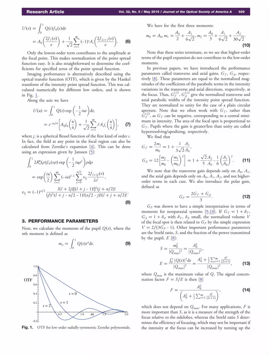
Imaging performance is alternatively described using theoptical transfer function (OTF), which is given by the Hankeltransform of the intensity point spread function. This was cal-culated numerically for different low orders, and is shownin Fig. 1.

Along the axis we have

U !u" #Z

1

0Q!t" exp

"!1

2iut

#dt;

# e!iu!4$A0j0

"u4

#$

1!!!2

pX!

s#1

isAsjs

"u4

#%; (7)

where js is a spherical Bessel function of the first kind of order s.In fact, the field at any point in the focal region can also becalculated from Zernike’s expansion [4]. This can be doneusing an expression given by Janssen [5]:

Z1

02R0

n!!"J0!v!" exp"!1

2iu!2

#!d!

# exp

"iu2

#X!

l#1

!!iu"l!1Xn!2

j#0

vlj2J l$2j!v"

l vl;

vl j # !!1"n!2l!l $ 2j"%!l $ j ! 1"!&2!j$ n!2"!

!j!"2!l $ j ! n!2 ! 1"!!n!2 ! j"!!l $ j$ n!2"!:

(8)

3. PERFORMANCE PARAMETERSNext, we calculate the moments of the pupil Q!t", where thenth moment is defined as

mn #Z

1

0Q!t"tndt : (9)

We have for the first three moments:

m0 # A0; m1 #A0

2$

A1

6!!!2

p ; m2 #A0

3$

A1

6!!!2

p $A2

30!!!2

p :

(10)Note that these series terminate, so we see that higher-order

terms of the pupil expansion do not contribute to the low-ordermoments.

In previous papers, we have introduced the performanceparameters called transverse and axial gains, GT , GA, respec-tively [8]. These parameters are equal to the normalized mag-nitudes of the coefficients of the parabolic terms in the intensityvariations in the transverse and axial directions, respectively, atthe focus. Thus, G1!2

T , G1!2A give the normalized transverse and

axial parabolic widths of the intensity point spread function.They are normalized to unity for the case of a plain circularaperture. Note that we often work with GT , rather thanG1!2

T , as GT can be negative, corresponding to a central mini-mum in intensity. The area of the focal spot is proportional toGT . Pupils where the gain is greater/less than unity are calledhyperresolving/apodizing, respectively.

We find that

GT #2m1

m0# 1$

1

3!!!2

pA1

A0;

GA # 12

$m2

m0!"m1

m0

#2%# 1$

!!!2

p

5

A2

A0!1

6

"A1

A0

#2

: (11)

We note that the transverse gain depends only on A0, A1,and the axial gain depends only on A0, A1, A2, and not higher-order terms in each case. We also introduce the polar gain,defined as

GP #2GT $ GA

3: (12)

GP was shown to have a simple interpretation in terms ofmoments for nonparaxial systems [9,10]. If GT # 1$ "T ,GA # 1$ "A with "T , "A small, the normalized volume Vof the focal spot is then related to GP by the simple expressionV # 2!!3GP ! 1". Other important performance parametersare the Strehl ratio, S, and the fraction of the power transmittedby the pupil, E [8]:

S #m2

0

jQmaxj2#

A20

jQmaxj2;

E #R10 jQ!t"j2dtjQmaxj2

#A20 $ 1

2

P!s#1

A2s

!2s$1"

jQmaxj2; (13)

where Qmax is the maximum value of Q . The signal concen-tration factor F # S!E is then [8]

F #A20"

A20 $ 1

2

P!s#1

A2s

!2s$1"

# ; (14)

which does not depend on Qmax. For many applications, F ismore important than S, as it is a measure of the strength of thefocus relative to the sidelobes, whereas the Strehl ratio S deter-mines the efficiency of focusing, which may not be important ifthe intensity at the focus can be increased by turning up the

0.5 1.0 1.5 2.0

–0.2

0.2

0.4

0.6

0.8

1.0

OTF

m

s = 0

s = 1s = 2

Fig. 1. OTF for low order radially-symmetric Zernike polynomials.

Research Article Vol. 32, No. 5 / May 2015 / Journal of the Optical Society of America A 929

incident power. In this paper we are mainly concerned withoptimization of F rather than S. We can now make a fewobservations. S and F both depend on the coefficients of allorders. GT is unaffected by the coefficients s > 1, but F is de-creased by increasing the magnitude of any coefficient s " 1.Thus, the optimum pupil for maximizing F for a given GThas As # 0, s > 1, i.e., the amplitude transmittance exhibitsa quadratic variation with radius, as we proved previously usingSchwartz’s inequality [2]. Then we find that GA decreases asGT increases. Defining the pupil as

Q!t" # !1 ! 2b" $ 2bt; 0 # b # 1; (15)

so that

A0 # 1 ! b; A1 #!!!2

pb; (16)

we find that, for 0 # b # 1,

S # !1 ! b"2; F #3!1 ! b"2

!3 ! 6b$ 4b2";

GT #!3 ! 2b"3!1 ! b"

; GA #!3 ! 6b$ 2b2"

3!1 ! b"2;

GP #!9 ! 16b$ 6b2"

9!1 ! b"2; (17)

agreeing with our previous results [2]. Then we also have therelationships between the parameters

F #1

1$ 3!GT ! 1"2;

S #1

%1$ 3!GT ! 1"&2; !1 ! GA" # 3!GT ! 1"2:

(18)

If, instead of maximizing F , we choose to maximize S, ifQmax occurs at the edge of the pupil, we have

S #A20"

A0 $ 1!!2

pPn

s#1 As

#2; (19)

which will increase if some coefficients are set to be negative. Sowe conclude that taking As # 0, s > 1 does not give the opti-mum condition. In fact, it has been shown many years ago thatthe optimum for maximizing S for a given transverse gain factoris a two-zone binary phase filter [11].

4. PUPIL OPTIMIZED FOR AXIAL RESOLUTIONNext we consider pupils that optimize the axial focusingperformance. We observe that GA is decreased for A1 $ 0, ir-respective of whether it is positive or negative. F is decreased byincreasing the magnitude of any coefficient s " 1, and we thenfind that the optimum pupil for maximizing F for a givenGA > 1 is when all coefficients except A0 and A2 are zero,in which case Q!t" is symmetrical about t # 1!2 and we have

GT # 1; GA # 1$!!!2

p

5

A2

A0; GP # 1$

!!!2

p

15

A2

A0;

F #1"

1$ 110

A22

A20

# ; S #1"

1$ 1!!2

p A2

A0

#2: (20)

If we define the pupil as

Q!t" # 1 ! 6bt $ 6bt2; (21)

where

A2

A0#

!!!2

pb

1 ! b; (22)

the performance parameters are

S # !1 ! b"2; 0 # b # 1; F #5!1 ! b"2

5 ! 10b$ 6b2;

GT # 1; GA #5 ! 3b5!1 ! b"

; GP #15 ! 13b15!1 ! b"

: (23)

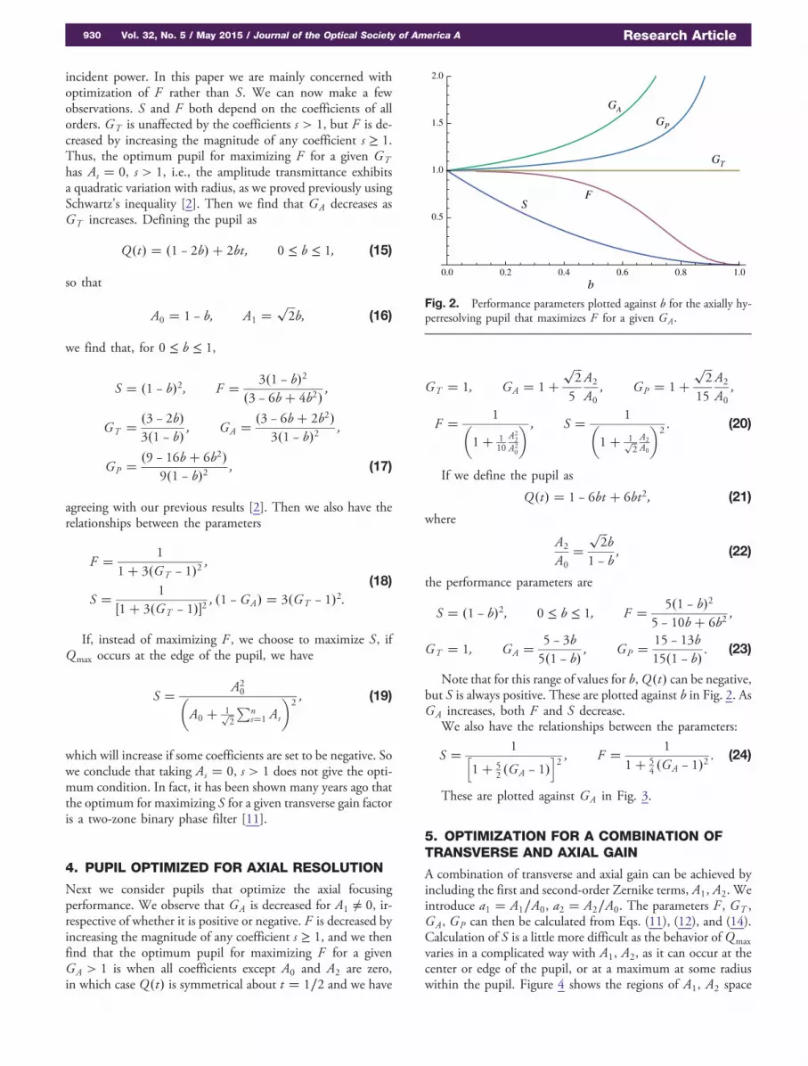
Note that for this range of values for b,Q!t" can be negative,but S is always positive. These are plotted against b in Fig. 2. AsGA increases, both F and S decrease.

We also have the relationships between the parameters:

S #1h

1$ 52 !GA ! 1"

i2; F #

1

1$ 54 !GA ! 1"2

: (24)

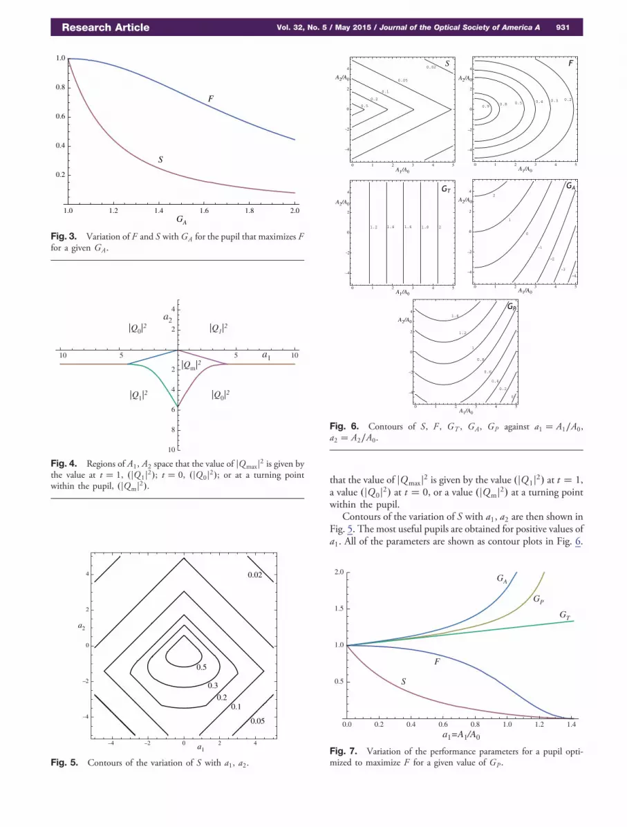
These are plotted against GA in Fig. 3.

5. OPTIMIZATION FOR A COMBINATION OFTRANSVERSE AND AXIAL GAINA combination of transverse and axial gain can be achieved byincluding the first and second-order Zernike terms, A1, A2. Weintroduce a1 # A1!A0, a2 # A2!A0. The parameters F , GT ,GA, GP can then be calculated from Eqs. (11), (12), and (14).Calculation of S is a little more difficult as the behavior of Qmax

varies in a complicated way with A1, A2, as it can occur at thecenter or edge of the pupil, or at a maximum at some radiuswithin the pupil. Figure 4 shows the regions of A1, A2 space

0.0 0.2 0.4 0.6 0.8 1.0

0.5

1.0

1.5

2.0

b

GT

GA

GP

SF

Fig. 2. Performance parameters plotted against b for the axially hy-perresolving pupil that maximizes F for a given GA.


that the value of jQmaxj2 is given by the value !jQ1j2" at t # 1,a value !jQ0j2" at t # 0, or a value !jQmj2" at a turning pointwithin the pupil.

Contours of the variation of S with a1, a2 are then shown inFig. 5. The most useful pupils are obtained for positive values ofa1. All of the parameters are shown as contour plots in Fig. 6.

1.0 1.2 1.4 1.6 1.8 2.0

0.2

0.4

0.6

0.8

1.0

GA

S

F

Fig. 3. Variation of F and S withGA for the pupil that maximizes Ffor a given GA.

10 5 5 10

10

8

6

4

2

2

4

|Qm|2

|Q1|2

|Q0|2|Q1|

2

|Q0|2

a2

a1

Fig. 4. Regions of A1, A2 space that the value of jQmaxj2 is given bythe value at t # 1, !jQ1j2"; t # 0, !jQ0j2"; or at a turning pointwithin the pupil, !jQmj2".

–4 –2 0 2 4

–4

–2

0

2

4

0.5

0.30.2

0.1

0.05

0.02

a1

a2

Fig. 5. Contours of the variation of S with a1, a2.

0 1 2 3 4 5

–4

–2

0

2

4

0 1 2 3 4 5

0

2

4

0 1 2 3 4 5

0

2

4

0 1 2 3 4 5

0

2

4

0 1 2 3 4 5

0

2

4

–4

–2

–4

–2

–4

–2

–4

–2

A1/A0

A1/A0

A1/A0

A1/A0 A1/A0

A2/A0A2/A0

A2/A0A2/A0

A2/A0

Fig. 6. Contours of S, F , GT , GA, GP against a1 # A1!A0,a2 # A2!A0.

0.0 0.2 0.4 0.6 0.8 1.0 1.2 1.4

0.5

1.0

1.5

2.0

a1=A1/A0

GT

GA

GP

S

F

Fig. 7. Variation of the performance parameters for a pupil opti-mized to maximize F for a given value of GP .


Appropriate choice of a1, a2 can result in a pupil that in-creases both GT and GA. As an example, we can maximize Ffor a given value of the polar gain GP . This optimization occurswhen the contours of F and GP are parallel, i.e., when!%F!%a1"!%GP!%a2" # !%F!%a2"!%GP!%a1" [12], giving thecondition

a2 #!!!2

pa1!!!

2p

! a1: (25)

The resulting variation of the different parameters with a1 isthen as shown in Fig. 7, and the amplitude transmittance of thepupil is shown in Fig. 8. The amplitude goes negative fora1 > 0.931, indicating a phase change of #. Obviously sucha pupil filter is more difficult to fabricate than one that is alwayspositive, but the value of F has already dropped almost to a halfif this is the case. At the values a1 # 0.931, a2 # 2.72, we haveF # 0.531, S # 0.078, GT # 1.22, GA # 1.63, GP # 1.36.

The variations in the normalized intensity in the focal planeand along the optical axis for three derived pupils are shown inFig. 9. Pupil (a) is a transverse hyperresolving pupil designed togive a flat axial behavior, i.e., to have a large depth of focus. Theperformance parameters are GT # 1.577, GA # 0, F # 0.5,S # 0.134. It can be considered to be an approximation to aBessel beam. Pupil (b) is an axially hyperresolving pupil withGA # 1.5. Other parameters for this case are GT # 1,F # 0.762, S # 0.198. Pupil (c) is the 3D hyperresolvingpupil with GP # 1.36 mentioned earlier.

6. DISCUSSION

Expanding the pupil function into Zernike components is aflexible approach for designing filters for different applications.In general, both the modulus and phase of the pupil functioncan be specified in this way. Here we have found the optimumradially symmetric pupil for giving the greatest signal concen-tration factor for a given width of the transverse point spreadfunction (defined by the second moment width). The opti-mum is an amplitude filter. The signal concentration factoris higher than for a pure phase filter, as the amplitude maskabsorbs some light that would otherwise contribute to the outerrings. We have also found the optimum pupil for giving thegreatest signal concentration factor for a given width of the axialpoint spread function. Finally, we considered more compli-cated pupil functions that can control both the transverseand axial behavior, and found the pupil that optimizes the sig-nal concentration factor for a given polar gain. We anticipatethat the expansion can be used for investigating a wide range ofdifferent pupil filter designs.

REFERENCES

1. M. Martinez-Corral and G. Saavedra, “The resolution challenge in 3Doptical microscopy,” Prog. Opt. 53, 1–67, (2009).

2. C. J. R. Sheppard, “Optimization of pupil filters for maximal signalconcentration factor,” Opt. Lett. 40, 550–553 (2015).

3. H. Osterberg and E. W. Wilkins, Jr., “The resolving power of a coatedobjective,” J. Opt. Soc. Am. 39, 553–557 (1949).

4. M. Born and E. Wolf, Principles of Optics, 5th ed. (Pergamon,1975).

5. J. E. M. Janssen, “Extended Nijboer–Zernike approach for thecomputation of optical point-spread functions,” J. Opt. Soc. Am. A19, 849–857 (2002).

6. C. J. R. Sheppard, S. Campbell, and M. D. Hirschhorn, “Zernikeexpansion of separable function of Cartesian coordinates,” Appl.Opt. 43, 3963–3966 (2004).

7. M. Abramowitz and I. A. Stegun, Handbook of MathematicalFunctions (Dover, 1965).

8. C. J. R. Sheppard and Z. S. Hegedus, “Axial behavior of pupil planefilters,” J. Opt. Soc. Am. A 5, 643–647 (1988).

0.0 0.2 0.4 0.6 0.8 1.0

0.2

0.4

0.6

0.8

1.0

P(!)

!

a1=0.931

0.4

0.8

0

Fig. 8. Pupil optimized to maximize F for a given value of GP , fordifferent values of the parameter a1. The pupil goes negative fora1 > 0.931.

2 4 6 8 10

0.2

0.4

0.6

0.8

1.0

v

I/I0

(a)

abc

5 10 15 20

0.2

0.4

0.6

0.8

1.0

u(b)

I/I0

a

b

c

Fig. 9. (a) Transverse and (b) axial intensity point spread functionsfor different pupils. The case of a plain aperture is shown in the dashedblack line. The other three cases are: a, axially hyperresolving; b, 3Dhyperresolving; and c, transverse hyperresolving and axially flat.


9. C. J. R. Sheppard, “Filter performance parameters for high-aperturefocusing,” Opt. Lett. 32, 1653–1655 (2007).

10. C. J. R. Sheppard, M. A. Alonso, and N. J. Moore, “Localizationmeasures for high-aperture wavefields based on pupil moments,”J. Opt. A Pure Appl. Opt. 10, 033001 (2008).

11. J. E. Wilkins, Jr., “The resolving power of a coated objective II,”J. Opt. Soc. Am. 40, 222–224 (1950).

12. C. J. R. Sheppard, J. Campos, J. C. Escalera, and S.Ledesma, “Two-zone pupil filters,” Opt. Commun. 281, 913–922(2008).


zernike expansion of pupil filters: optimization of the signal concentration factor

Documents