1

Worst-Case Jamming on MIMO Gaussian ChannelsJie Gao, Sergiy A. Vorobyov, Senior Member, IEEE,

Hai Jiang, Senior Member, IEEE and H. Vincent Poor, Fellow, IEEE

Abstract—Worst-case jamming of legitimate communicationsover multiple-input multiple-output Gaussian channels is studiedin this paper. A worst-case scenario with a ‘smart’ jammer thatknows all channels and the transmitter’s strategy and is onlypower limited is considered. It is shown that the simplificationof the system model by neglecting the properties of the jammingchannel leads to a loss of important insights regarding the effectsof the jamming power and jamming channel on optimal jam-ming strategies of the jammer. Without neglecting the jammingchannel, a lower-bound on the rate of legitimate communicationsubject to jamming is derived, and conditions for this boundto be positive are given. The lower-bound rate can be achievedregardless of the quality of the jamming channel, the powerlimit of the jammer, and the transmit strategy of the jammer.Moreover, general forms of an optimal jamming strategy, onthe basis of which insights into the effect of jamming powerand jamming channel are exposed, are given. It is shown thatthe general forms can lead to closed-form optimal jammingsolutions when the power limit of the jammer is larger thana threshold. Subsequently, the scenario in which the effect ofjamming dominates the effect of noise (the case of practicalinterest) is considered, and an optimal jamming strategy isderived in closed-form. Simulation examples demonstrate lower-bound rates, performance of the derived jamming strategy, andan effect of inaccurate channel information on the jammingstrategy.

Index Terms—Closed-form solution, lower-bound rate,multiple-input multiple-output Gaussian channel, optimization,worst-case jamming.

I. INTRODUCTION

Reliability and security are major concerns in modern wire-

less communications [1]- [6]. Due to the rapid development

of wireless communications, threats to reliable and secure

communications are becoming more prevalent as wireless

communication networks of different scales containing devices

for different purposes become more common and widespread.

One of major threats to wireless communications is jam-

ming. Jamming aims at degrading the quality of communica-

Manuscript submitted November 24, 2014; revised May 28, 2015; acceptedJuly 5, 2015. The associate editor coordinating the review of this manuscriptand approving it for publication was Dr. Gesualdo Scutari.

Copyright (c) 2015 IEEE. Personal use of this material is permitted. How-ever, permission to use this material for any other purposes must be obtainedfrom the IEEE by sending a request to pubs-permissions@ieee.org.

J. Gao and H. Jiang are with the Department of Electrical and ComputerEngineering, University of Alberta, Edmonton, AB T6G 2V4, Canada (e-mail:jgao3@ualberta.ca, hai1@ualberta.ca).

S. A. Vorobyov is with the Department of Signal Processing and Acoustics,School of Electrical Engineering, Aalto University, PO Box 13000 FI-00076AALTO, Finland (e-mail: sergiy.vorobyov@aalto.fi).

H. V. Poor is with the Department of Electrical Engineering, PrincetonUniversity, Princeton, NJ, USA (e-mail: poor@princeton.edu).

Some preliminary results of this paper have been presented atICASSP 2014, Florence, Italy.

This research was supported in part by the Natural Sciences and Engineer-ing Research Council of Canada and by the U.S. National Science Foundationunder Grant CMMI-1435778.

tion or disrupting the information transmission in a commu-

nication system by directing energy toward the target receiver

in a destructive manner [7]. A jamming attack is particularly

effective because it is easy to launch using low-cost and small-

sized devices while causing very significant disruption [8]. The

threat of jamming has been studied in many works [9]- [15],

and one of the relevant research interests in this area is to

investigate optimal jamming strategies from the perspective of

a jammer [8], [12]–[16]. Such a perspective helps to reveal the

worst-case effects of jamming on legitimate communications.

In the sequel, the terms of “worst-case jamming” and “optimal

jamming” are used interchangeably where “worst-case jam-

ming” is from the perspective of the legitimate communication

and “optimal jamming” is from the perspective of the jammer.

The study of worst-case jamming is more complicated

when the jammer has multiple antennas. In such cases, the

jammer is able to use more subtle jamming strategies by

adjusting the jamming signal across its antennas and conse-

quently enhancing the effectiveness of jamming on the target

communication. As a result, it is of interest to investigate

worst-case jamming in the scenario in which the jammer and

the legitimate transceivers all employ multiple antennas and

to establish the limits of the jammer in terms of degrading the

quality of the legitimate communication in such situations.

Related problems have been investigated in the literature

[17]- [20]. It is shown in [17] that without knowledge of

the target signal or its covariance, the jammer can only use

basic strategies of allocating power uniformly or maximizing

the total power of the interference at the target receiver. In

[18], the transmit strategies of a legitimate transmitter and a

jammer on a Gaussian multiple-input multiple-output (MIMO)

channel are investigated under a game-theoretic model with a

general utility function. It is assumed that the jammer and

the legitimate transmitter have the same level of channel state

information (CSI), i.e., both uninformed, both with statistical

CSI, or both with exact instantaneous CSI. Optimal transmis-

sion strategies of the legitimate transmitter and the jammer

are represented as solutions to different optimization problems

for different types of CSI. The optimal jamming of a jammer

on MIMO multiple access and broadcast channels with the

covariance of the target signal and all channel information

available at the jammer is studied in [19] based on game

theory. Some properties of the optimal jamming strategies are

characterized through the analysis of the Nash equilibrium

of the game. A necessary condition for optimal jamming on

MIMO channels with arbitrary inputs when the covariance of

the target signal and all channel information are available at

the jammer is derived in [20]. For the case of a Gaussian

target signal, the solution of optimal jamming is given in

closed-form. However, it is derived without considering the

2

jamming channel, i.e., the jamming channel is assumed to be

equal to an identity matrix. As a result, the system model

is oversimplified by implicitly assuming that the received

jamming signal at the target receiver is exactly the same as

the transmitted jamming signal at the jammer. With a similar

assumption, a game between a MIMO radar and a jammer

is investigated in [21] and the strategies of both sides are

analyzed. The worst-case noise, comprised of both multi-user

interference and Gaussian noise, in a multi-user cellular system

is investigated in [22]. The authors of [22] study the worst-case

noise under constraints on its trace, eigenvalues, or diagonal

elements, and the capacity of the considered system is derived

by solving corresponding minimax problems on the noise and

transmit covariance matrices.

With the objective of providing a general solution without

oversimplification of the system model, this work addresses

the problem of characterizing the worst-case effect of jamming

on MIMO Gaussian channels and finds an optimal jamming

strategy of the jammer in the jammer-dominant regime, i.e.,

where jamming dominates noise at the target receiver. Without

the assumption of the jamming channel being equal to an

identity matrix, it can be shown that finding the optimal jam-

ming strategy does not reduce to a power allocation problem

anymore. Moreover, unlike the case in which the optimal so-

lution can be found in closed-form with the assumption on the

jamming channel being equal to an identity matrix, the optimal

jamming solution without this assumption may not exist in

closed-form for non-diagonal jamming channels depending on

the jamming power limit. The main contributions of this work

are as follows.1

First, we show that there is a lower-bound on the rate that

the legitimate communication can achieve regardless of the

quality of the jamming channel, the power limit of the jammer,

and the transmit strategy of the jammer. We give an expression

for the lower-bound rate as well as a condition that assures

the lower-bound rate is positive. Moreover, it is shown that

a non-zero lower-bound rate is not necessarily a result of the

jamming channel having lower rank than (or spanning a subset

of) the legitimate channel. It also depends on how the jamming

power is directed toward the target signal at the receiver via

the jamming channel. This result was not obtained in previous

works in which the jamming channel is assumed to be equal

to an identity matrix.

Second, we characterize general forms of the optimal jam-

ming strategy. Based on the general forms, it is shown that

neglecting the jamming channel leads to a loss of important

insight into the jamming strategy, i.e., the jammer should

generally allocate more power on weak subchannels in the

optimal strategy. Moreover, we show that when the power

limit of the jammer is larger than a threshold, the optimal

jamming strategy can be obtained in closed-form from the

general forms. It includes the scalar solutions in [20] and [21]

as special cases in which the jamming channel is equal to an

identity matrix. When a closed-form solution is not available,

insights into the jamming strategy can still be provided based

on the characteristics of the general forms.

1Some very preliminary results have been presented in [23].

Third, we focus on the practical scenario in which the

effect of jamming dominates the effect of noise and find a

closed-form optimal jamming strategy in the jammer-dominant

regime. It is shown that there is a unified closed-form solution

for the optimal jamming strategy in this regime. Moreover, it is

shown that the proposed closed-form solution in the jammer-

dominant regime leads to performance very close to optimal

even for the scenarios in which the effect of jamming is not

dominant.

The rest of the paper is organized as follows. Section II

explains the system model considered in this work. The

problem of finding a lower-bound rate for the legitimate

transceiver and general forms of the optimal jamming strategy

is investigated in Section III where closed-form solutions

are derived when the power limit of the jammer exceeds a

threshold. The scenario in which the effect of jamming is

dominant over the effect of noise, i.e., in the so-called jammer-

dominant regime, is studied in Section IV and a closed-form

solution for the optimal jamming strategy is found. Section V

discusses simulation examples confirming the results obtained

in the previous sections, and Section VI concludes the paper.

Section VII “Appendix” provides proofs for the lemmas and

theorems.

II. SYSTEM MODEL

A legitimate transmitter with nt antennas sends a signal s to

a receiver with nr antennas. The elements of s are independent

and identically distributed Gaussian random variables with

zero means and covariance Qs. A jammer with nz antennas

attempts to jam the legitimate communication by transmitting

a jamming signal z to the receiver. Denote the channel from the

legitimate transmitter to the receiver as Hr (of size nr × nt)

and the jamming channel from the jammer to the receiver

as Hz (of size nr × nz). The case of block fading channels

is considered here. Therefore, the channels remain constant

during a fading block. In the presence of the jamming signal,

the received signal at the receiver can be expressed as

y = Hrs+Hzz+ n, (1)

where n is Gaussian noise with zero mean and covariance σ2I.

Here I denotes the identity matrix of an appropriate size. Note

that given the Gaussian channel and Gaussian target signal,

the worst-case jamming signal should also be Gaussian [24].

Denote the covariance of z as Qz. Then the information rate

of the legitimate communication in the presence of jamming

is expressed as

RJ = log |I+HrQsHH

r (HzQzHH

z + σ2I)−1|, (2)

where | · | and (·)H denote the determinant and the Hermitian

transpose, respectively. The jammer aims at decreasing the

above rate as much as possible given its power limit Pz.

If the jamming channel Hz is unknown, the jammer has

no better strategy than uniformly allocating its transmission

power, i.e., Qz = Pz/nz · I. If the jammer knows Hz but

not Qs and/or Hr, it can maximize the jamming power at

the receiver, i.e., maximize TrHzQzHHz [17], where Tr·

denotes the trace. In both of the above two cases, the optimal

3

TABLE I: Table of Notations

X matrix

TrX the trace of X

|X| the determinant of X

X ≻ 0 X is positive definite

X 0 X is positive semidefinite

XH the Hermitian transpose of X

Ur,Uz the unitary matrix consisting of left-singular vectors of Hr,Hz

Vr,Vz the unitary matrix consisting of right-singular vectors of Hr,Hz

Ωr,Ωz the diagonal matrix consisting of singular values of Hr,Hz

Ωr, Ωz the block of Ωr,Ωz consisting of only positive singular values

UX the unitary matrix consisting of eigenvectors of X

ΛX the diagonal matrix consisting of eigenvalues of X

ΛX the block of ΛX consisting of only positive eigenvalues

UX1 the columns of UX corresponding to ΛX

UX2 the columns of UX corresponding to zero eigenvalues

strategy of the jammer is well-known. In this paper, similar

to [19], [20], and [21], the jammer is assumed to have the

knowledge of Hr, Hz, and Qs but not s. For example, the

jammer may obtain information on Hr and Hz when it is

also capable of eavesdropping and the channels are reciprocal.

The jammer is not able to perform correlated jamming [25].

However, the jammer can use the available knowledge to find

the optimal Qz such that the rate (2) is minimized. It should

be noted that the worst-case perspective of the study aims at

understanding a limit on what can be achieved by jamming and

the resulting jamming strategy. Therefore, the practicality of

the results lies in the fact that, given a specific problem setup,

the obtained results can be used to understand what would be

the effect of jamming in the worst-case. It should be noted

that the assumption on the availability of Hz is weaker than

the assumption imposed by neglecting the jamming channel

as considered in [20] and [21]. In the latter case, the jamming

channel has been assumed not only to be known but also to

be equal to an identity matrix.

Given the above system model, we are especially interested

in the case in which the effect of jamming on the received

legitimate signal dominates the effect of the noise. It is worth

noting, however, that the noise term in (2) cannot be simply

neglected in general due to the fact that the term HzQzHHz can

be rank-deficient, e.g., when Hz does not have full row rank.

It will also be shown later that the optimal form of HzQzHHz

is rank-deficient when HrQsHHr is rank-deficient. There was

no need to address these cases in [20] and [21] where the

jamming channel Hz was assumed to be I. As a result, while

we focus on the case in which jamming dominates noise, we

do not neglect the noise term σ2I. Instead, we define a jammer-

dominant regime which will be explained in detail later and

find an optimal jamming strategy in this regime.

The symbols and notations used in this paper are summa-

rized in Table I for clarity of presentation.

III. LOWER-BOUND RATE AND GENERAL FORMS OF

OPTIMAL JAMMING STRATEGY

In this section, we first investigate the effect of jamming on

the legitimate communication with the objective of finding a

part of the information rate of the legitimate communication

which is unaffected by jamming. This unaffected part of the

information rate is of interest because it leads to results on the

lower-bound rate of the legitimate communication. Then, we

study general forms of the optimal jamming strategy, which are

fundamental for finding closed-form solutions of the optimal

jamming strategy.

A. Lower-bound rate for legitimate communication

Given the system model, an optimal jamming strategy can

be found by solving the following problem2:

minQz

RJ (3a)

s.t. TrQz ≤ Pz. (3b)

With only one pair of transceivers, the above problem is a

basic jamming problem on a MIMO channel. While the above

problem is convex, our objective is to gain insights into the

optimal jamming strategy and the corresponding effect on

the legitimate communication, which cannot be provided by

a numerical solution. We also aim at finding a closed-form

solution for the optimal jamming strategy when possible.

Note that problem (3) can be extended to a maxmin

problem in which, given the optimal jamming strategy, the

legitimate transmitter aims at maximizing its information rate

under jamming. Such extension is straightforward since the

optimal strategy of the legitimate transmitter is to consider

the jamming signal as noise and use waterfilling to obtain

its optimal transmit covariance. Therefore, our focus in the

sequel will be on deriving the optimal jamming strategy of

the jammer.

Denote the singular value decomposition (SVD) of Hz as

Hz = UzΩzVHz and the rank of Hz as rz. The matrices

Uz, Ωz, and Vz are of sizes nr × nr, nr × nz, and nz × nz,

respectively. Denote the SVD of Hr as Hr = UrΩrVHr . The

matrices Ur, Ωr, and Vr are of sizes nr × nr, nr × nt, and

nt × nt, respectively. Define

B , UH

z HrQsHH

r Uz. (4)

Note that B has the same rank as HrQsHHr . Using the

definition of B and the SVD of Hz, the objective function

in (2) can be rewritten as

RJ = log |I+B(ΩzQzΩH

z + σ2I)−1|, (5)

where

Qz , VH

z QzVz. (6)

Lemma 1: If we denote B using blocks such that

B =

[

rz nr−rz

rz B11 B12

nr−rz B21 B22

]

, (7)

and define

B , B11 −B12(σ2I+B22)

−1B21, (8)

2The positive semi-definite constraint Qz 0 is assumed by default andit is omitted for brevity throughout this paper.

4

then B is positive definite (PD) if B is PD.

Proof: See Subsection VII-A in the Appendix.

Before solving the optimization problem (3), it is essential

to express the objective function of problem (3) in a different

form so as to reveal the optimal structure of Qz. Denote the

diagonal matrix Ωz using blocks as

Ωz ,

[

rz nz−rz

rz Ωz 0

nr−rz 0 0

]

, (9)

where Ωz is an rz × rz diagonal matrix made up of the

positive diagonal elements of Ωz, and 0 denotes an all-

zero matrix of an appropriate size. It can be seen that the

allocation of jamming power should be limited to at most rzdimensions corresponding to the rz non-zero singular values

of Ωz. Indeed, allocating jamming power anywhere else has no

effect on the received signal and only leads to jamming power

waste. As a result, Qz should adopt the following form:

Qz =

[

rz nz−rz

rz Q′

z Γz

nz−rz ΓHz 0

]

, (10)

where Q′

z and Γz are to be determined. The matrix Γz does

not affect the rate of RJ in (5). Therefore, Γz is set to be 0

for simplicity and consequently

Qz =

[

rz nz−rz

rz Q′

z 0

nz−rz 0 0

]

. (11)

Let us define a new matrix Ωz given as

Ωz ,

[

rz nr−rz

rz Ωz 0

nr−rz 0 I

]

. (12)

The channel matrix Ωz has size nr × nr, which is larger than

the size of Ωz if nr > nz, smaller than the size of Ωz if

nr < nz, and has the same size as Ωz if nr = nz. Also define

the following new jamming covariance matrix Qz:

Qz ,

[

rz nr−rz

rz Q′

z 0

nr−rz 0 0

]

, (13)

where Q′

z is the same as in (10).

With the above definitions of Ωz and Qz, it can be seen that

ΩzQzΩHz in (5) is equal to ΩzQzΩz (note that ΩH

z = Ωz).

As a result, the rate in (5) can be equivalently rewritten as

RJ = log |I+B(ΩzQzΩz + σ2I)−1|. (14)

Therefore, we consider Ωz and Qz as the equivalent channel

matrix and the equivalent jamming covariance matrix to Ωz

and Qz, respectively. The advantage of solving the optimiza-

tion problem (3) using the above equivalent form of the

objective function is that Ωz in (14) is always PD and therefore

can be extracted from the inverse term, which simplifies the

solution finding procedure.

Using the above observations and equations (6) and (11) it

can be seen that the optimal form of Qz is

Qz = Vz

[

Q′

z 0

0 0

]

VH

z , (15)

where the two diagonal blocks in the block diagonal matrix

have sizes rz × rz and (nz − rz)× (nz − rz), respectively.

Lemma 2: A lower-bound rate that can be achieved given

the transmit strategy of the legitimate transceiver Qs and the

legitimate channel Hr is

R0 = log

∣

∣

∣

∣

I+1

σ2B22

∣

∣

∣

∣

, (16)

while the minimization of RJ with respect to Qz is equivalent

to the minimization of

RJ = log |I+ Ω−1

z BΩ−1

z (Q′

z +D)−1|, (17)

where D , σ2Ω−2z .

Proof: See Subsection VII-B in the Appendix.

Since B22 0 (which follows from (7) and the fact that

B 0), it can be seen from Lemma 2 that R0 = 0 only when

(1) nr = rz or (2) nr > rz and B22 = 0.

In the first case, the jammer has at least the same number of

antennas as the receiver and the jamming channel has full rank.

Therefore, the column space of Hz includes the column space

of Hr as a subset. Thus, the jammer can spread its jamming

power on all the data streams (on the eigenchannels of Hr)

of the legitimate communication. As a result, the legitimate

communication does not have a positive lower-bound data rate.

In the second case, B22 = 0 implies two things. First,

the received legitimate signal has a rank no greater than rz.

Second, using (4) and (7), it can be seen that B22 = 0 leads

to a requirement on how the jamming channel directs the

jamming signal to the receiver. Specifically, for R0 to be 0, the

columns of Uz corresponding to the zero eigenvalues of Hz

must belong to the null space of the received signal covariance

HrQsHHr . Consequently, the jamming power must be directed

so that all data streams of the legitimate communication are

subject to jamming.

The above two cases can be summarized as a sufficient

and necessary condition for R0 to be 0. Specifically, the

lower-bound rate is zero if and only if the span of the

jamming channel includes the span of HrQsHHr as a subspace.

Otherwise, the jammer cannot jam all the data streams of the

legitimate communication and the legitimate transceiver can

achieve a positive minimum rate through the data streams

which are not jammed. Note that even if the rank of the

jamming channel is higher than that of the legitimate channel

(and thereby the jammer has more spatial degrees of freedom),

the legitimate communication may still achieve a positive

lower-bound rate depending on how the jamming signal is

directed.

Following the above discussion, conditions for the lower-

bound rate R0 to be positive depending on the rank of B can

be given.

Lemma 3: Denote rB as the rank of B. The following

results regarding R0 > 0 and rB hold:

1) R0 must be positive if rB > rz.

5

2) R0 can be positive as long as rB > 0.

Proof: See Subsection VII-C in the Appendix.

As can be seen from (4) and (16), the lower-bound rate R0

does not depend on the jamming signal Q′

z, or either of Ωz

and Vz in the jamming channel. The only factors related to

jamming that the lower-bound rate depends on are the rank rzand the matrix Uz. As a result, given rz, the rate R0 does

not depend on the specific jamming signal or the channel

gain of the jamming channel but rather on how the jamming

signal is directed towards the receiver, i.e., the alignment of the

jamming signal towards the received legitimate signal. Given

the above fact, it is of interest to find the Uz that leads to the

smallest R0 given HrQsHHr .

Lemma 4: Given HrQsHHr , R0 is minimized when the

last3 nr − rz columns of Uz consist of the eigenvectors

corresponding to the smallest nr−rz eigenvalues of HrQsHHr .

If the legitimate transmitter uses waterfilling, R0 is minimized

when the last nr−rz columns of Uz consist of the last nr−rzcolumns of Ur.

Proof: See Subsection VII-D in the Appendix.

It should be noted that minimizing R0 is only minimizing

the lower-bound rate. It is different from minimizing the infor-

mation rate of the legitimate communication under jamming,

which we will study next.

B. General forms of optimal jamming strategies

Given the above lemmas, we next solve the problem (3) by

finding the optimal Q′

z in (15). Denote

A , Ω−1

z BΩ−1

z . (18)

The following theorem investigates the optimal form of Q′

z

when A is PD .

Theorem 1: In the case in which A ≻ 0, the general form

of the optimal Q′

z for the jamming problem (3) is given by

Q′

z = A1

2

(

A−1

2 (λI+ Z)−1A−1

2 +1

4I

)1

2

A1

2 −1

2A−D,

(19)

where λ is chosen so that TrQ′

z = Pz and Z is a positive

semi-definite (PSD) matrix that satisfies TrZQ′

z = 0.

Proof: See Subsection VII-E in the Appendix.

The parameters λ and Z in (19) are in fact the Lagrange

multipliers associated with the constraints TrQ′

z ≤ Pz and

Q′

z 0, respectively. As mentioned earlier, a special case

of the problem (3) that assumes the jamming channel Hz to

be the identity matrix I has been investigated in [20] as well

as in the game theoretic setup for MIMO radar application

[21]. Under this special assumption, Uz, Ωz, and VHz are

all equal to I. Consequently, A and Ωz simplify to B and

I, respectively. With the above simplifications, the problem

of finding an optimal jamming strategy reduces to finding an

optimal jamming power allocation, and the solution is given

in a scalar form.

It should be noted that neglecting the jamming channel leads

to a loss of insight into the effect of the jamming channel

3By ‘last n columns’ in an eigenvector matrix, we refer to the n columnsof eigenvectors corresponding to the n smallest eigenvalues.

on the jammer’s strategy. Before showing the effect of the

jamming channel, we briefly explain the difference in finding

the solution with and without considering the jamming channel

as follows. Without considering the jamming channel, the

problem becomes minimizing the following objective function:

RJ = log |I+ Ω−1

z BΩ−1

z (Q′

z + I)−1| (20)

subject to the jammer’s power limit. If we create a new variable

X such that X = Q′

z+ I, it is not difficult to obtain a closed-

form solution for X subject to the power constraint TrX ≤TrQ′

z + I. The optimal solution for Q′

z is then X − I if

the result is PSD. When the result is indefinite, we can still

obtain a closed-form solution for Q′

z from the solution for X

based on projection, i.e., projecting the negative eigenvalues of

Q′

z to zero and reducing the positive eigenvalues accordingly.

This is possible because the eigenvalues of Q′

z are equal to

the eigenvalues of X minus 1 while the eigenvectors remain

the same. However, when the jamming channel is considered

and I in the brackets in (20) is replaced by D, the above-

mentioned method is not applicable anymore. Indeed, although

D is a diagonal matrix, it is in general impossible to know

the eigenvalues of X−D based on a non-diagonal matrix X.

Therefore, it may be impossible to find a closed-form solution

in general. However, the obtained general form of the optimal

jamming strategy in (19) can lead to the optimal closed-form

solution in special cases. The following remark provides an

example.

Remark 1: In the case in which A ≻ 0, there is a threshold

value for Pz, denoted by P ∗

z , such that when Pz > P ∗

z the

optimal Q′

z is a PD matrix given by

Q′

z = A1

2

(

1

λA−1 +

1

4I

)1

2

A1

2 −1

2A−D. (21)

The justification for the expression (21) when Q′

z is PD is

straightforward. Given the constraints TrZQ′

z = 0 and

Z 0 in Theorem 1, it holds true that Z = 0 if Q′

z is

PD. Substituting Z = 0 in (19) leads to (21). The threshold

P ∗

z is the trace of Q′

z when the minimum eigenvalue of Q′

z

in (21) approaches zero. The threshold P ∗

z can be determined

numerically given a specific problem although it cannot be

simply expressed as a function of other parameters. If we

search for λ0 such that the minimum eigenvalue of Q′

z in

(21) is 0 when λ is equal to λ0, and becomes positive when

λ becomes larger than λ0, the trace of Q′

z with λ substituted

by λ0 is equal to P ∗

z .

It should be noted that the solution (21) includes the scalar

solutions in [20] and [21] as special cases in which the

jamming channel is equal to an identity matrix.

The solution (21) can be used to demonstrate the effect

of the jamming channel on the optimal jamming strategy. In

order to isolate and reveal this effect of the jamming channel,

consider the case in which Hr, Qs, and correspondingly B

are equal to I. As a result, the target signal HrQsHHr at the

receiver is an identity matrix, and the effects of the variance of

the target signal and of the legitimate communication channel

on the jamming strategy are eliminated. In this case, using the

6

0.1

0.2

0.3

0.4

0.5 0

10

20

30

40

0

2

4

6

8

10

ω2/σ2 (dB)λ

f(ω

,λ,σ

2)

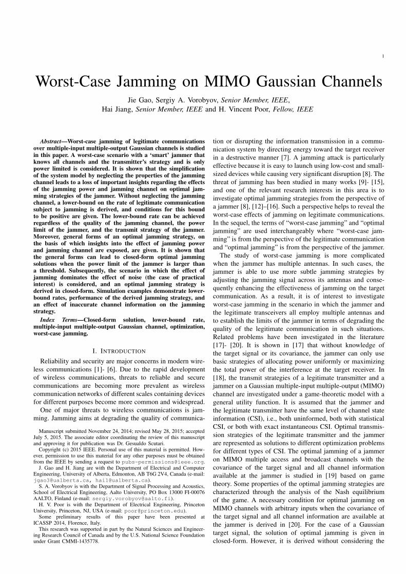
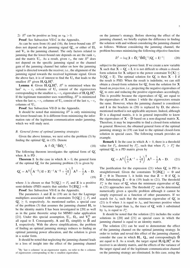
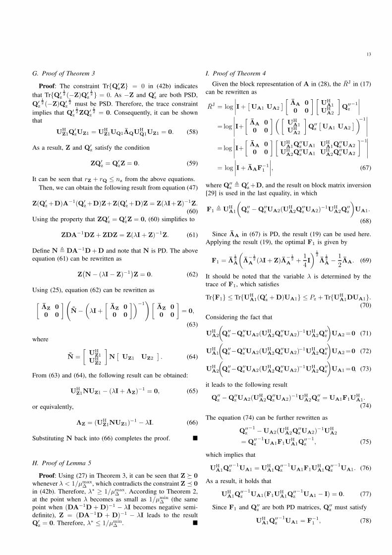
Fig. 1: Illustration of the effect of the jamming channel on the

optimal jamming strategy.

definition of A and D, Q′

z in (19) becomes

Q′

z =

(

1

λΩ−2

z +1

4Ω−4

z

)1

2

−1

2Ω−2

z − σ2Ω−2

z . (22)

In the above expression, Q′

z becomes a power allocation

matrix. The power allocation across the diagonal elements of

Q′

z depends on Ωz and is of interest. Following the form of

(22), a function f(ω, λ, σ2) can be defined as follows:

f(ω, λ, σ2) =

(

1

λω−2 +

1

4ω−4

)1

2

−1

2ω−2 − σ2ω−2. (23)

The plot of f(ω, λ, σ2) versus ω2 (σ2 is fixed at 0.01) and λ is

shown in Fig. 1, which explicitly demonstrates the following

effects of jamming channel on the optimal jamming strategy.

First, for a given power budget (fixing λ), the jammer allo-

cates more jamming power on the weak jamming subchannels

(corresponding to the small elements of Ωz) as compared

to its power allocated on the strong jamming subchannels

(corresponding to the large elements of Ωz). This can be

seen from Fig. 1 because a smaller ω generally leads to a

larger f(ω, λ, σ2) for a given λ. Although it seems counter-

intuitive that it is optimal for the jammer to use most of its

power on weak jamming subchannels, it should be noted that

the target is a signal transmitted through a MIMO channel

that has multiple data streams. While some streams might

be significantly reduced if the jammer allocates most of its

power on the strong jamming subchannels, the effect of such

a jamming strategy on other streams can be very limited

due to the combination of limited remaining jamming power

and weak jamming subchannels. Therefore, the jammer takes

advantage of the stronger jamming subchannels by achieving

a decent jamming effect with limited jamming power, and

achieves the overall optimality by allocating the remaining

power on the weaker subchannels.

Second, although in general more jamming power is al-

located on weak jamming subchannels, the jammer reduces

its power allocation on a subchannel when it becomes too

weak, reaching a certain threshold. This is intuitive since if the

most jamming power is allocated to the worst subchannel, a

subchannel with zero gain would be allocated with the largest

portion of the jammer’s power. This is clearly not optimal.

Therefore, as can be seen from Fig. 1, f(ω, λ, σ2) decreases

when ω2/σ2 becomes too small for a given power budget, or

equivalently, for a given λ.

Third, when the power limit of the jammer increases (or

equivalently, λ decreases), the majority of the extra power is

allocated on weak subchannels. This can also be seen from

Fig. 1 by comparing two curves with different values of λ.

The above insights in the optimal jamming strategy obtained

from exploring the general form (19), which leads to the

solution (21) and consequently (22) and (23), cannot be seen

if the jamming channel is neglected.

C. Characterization of Z and λ

In order to obtain more insights from the general form of the

optimal Q′

z in (19), the properties of Z and λ are investigated

in this subsection.

Theorem 2: Q′

z in (19) is PSD when

Z (DA−1D+D)−1 − λI. (24)

Moreover, Q′

z = 0 when the equality holds.

Proof: See Subsection VII-F in the Appendix.

Using Theorem 2 and Remark 1, Z can be easily found

for two special cases. The first special case is when Pz is

sufficiently large such that Q′

z is PD, and in such case Z = 0.

The second special case is when Pz approaches zero and as a

result Q′

z approaches 0. In this case, Z = (DA−1D+D)−1−λI. However, for all other possible Pz in between, Z and λare yet to be characterized.

Denote the ranks of Z and Q′

z by rZ and rQ, respectively,

and the eigenvalue decomposition (EVD) of Z as

Z =[

rZ rz−rZ

UZ1 UZ2

]

[

ΛZ 0

0 0

][

UHZ1

UHZ2

]

, (25)

and the EVD of Q′

z in (19) as

Q′

z =[

rQ rz−rQ

UQ1 UQ2

]

[

ΛQ 0

0 0

][

UHQ1

UHQ2

]

. (26)

The following theorem is in order.

Theorem 3: For all choices of Pz, rZ + rQ ≤ nz and the

Z in (19) must satisfy the following condition:

ΛZ = (UH

Z1(DA−1D+D)UZ1)−1 − λI. (27)

Proof: See Subsection VII-G in the Appendix.

Theorem 3 leads to several results that characterizes Z and

λ. An immediate result based on Theorem 3 is given in the

following remark.

Remark 2: Z in (19) always satisfies the condition that

UHZ1(DA−1D+D)UZ1 is diagonal.

Combining Theorems 2 and 3, a further characterization of

λ can also be obtained.

Lemma 5: Define λ∗ such that Q′

z in (21) is PD for all

λ < λ∗ and indefinite for all λ > λ∗. Denote the maximum

7

and minimum eigenvalues of DA−1D+D as µmax∆

and µmin∆

,

respectively. When Z 6= 0, it holds that 1/µmax∆

≤ λ∗ ≤1/µmin

∆.

Proof: See Subsection VII-H in the Appendix.

Summarizing the above results, the corresponding change

in Z and λ versus the jamming power Pz is identified. When

Pz is sufficiently large such that Q′

z is PD, then 0 < λ < λ∗

and Z = 0. As Pz decreases, λ increases. Meanwhile, ΛZ in

(27) gradually grows larger in size, and as a result the rank of

Z increases while the rank of Q′

z decreases. Ultimately, when

Pz approaches zero, λ approaches 1/µmin∆

and Z approaches

(DA−1D+D)−1 − λI while Q′

z approaches 0.

It should be noted that λ is different if the jamming

channel Hz is assumed to be I. In that case, Z is always

0 while λ varies from 0 (when the jamming power Pz is

infinite) to positive infinity (when the jamming power Pz is

0). Without considering the jamming channel, the parameter λis enough for adjusting the jamming strategy, which reduces

to a jamming power allocation strategy given a target signal.

However, when Hz is not equal to I, the jamming strategy

has to be adjusted according to not only the power limit

but also the jamming channel. The matrix Z can be seen

as the parameter to adjust the jamming strategy according

to the jamming channel, which explains why Z must always

satisfy (27) (in which D is a characterization of the jamming

channel).

The results in Theorem 2 and 3 can also be used for

obtaining an efficient suboptimal jamming solution which

requires a search over λ instead of solving semi-definite

programming problems. The main idea lies in the choice of

UZ1 in (27) among those which diagonalize DA−1D + D.

The details, however, are beyond the scope of this study.

D. The case when A 0

In the case in which A is PSD but not PD, assume that the

rank of A is rA. Denote the EVD of A as UAΛAUHA and

the block expression of A as

A =[

rA rz−rA

UA1 UA2

]

[

ΛA 0

0 0

][

UHA1

UHA2

]

. (28)

When A is PSD but not PD, the problem of minimizing

RJ subject to the jammer’s power constraint is not a strictly

convex problem. Therefore, the optimal solution is not neces-

sarily unique and the result in Theorem 1 cannot be directly

extended. The following theorem gives a general form of one

optimal Q′

z that minimizes RJ when A is a PSD matrix but

not PD.

Theorem 4: When A is PSD but not PD, a general form of

one optimal solution Q′

z to the jamming problem (3) is given

by

Q′

z =UA1

(

Λ1

2

A

(

Λ−

1

2

A (λI+ Z)−1Λ−

1

2

A +1

4I

)1

2

Λ1

2

A

−1

2ΛA

)

UH

A1 +UA2UH

A2DUA2UH

A2 −D, (29)

where λ is chosen so that TrQ′

z = Pz and Z is a PSD matrix

that satisfies ZQ′

z = 0.

Proof: See Subsection VII-I in the Appendix.

Note that although the expressions of the general forms (19)

and (29) are similar, the expression (29) cannot be directly

obtained from the results when A is a PD matrix. In fact,

finding the general form of the solution is more challenging

when A does not have full rank and, as a result, the solution is

not unique. Intuitively, the general form given in (29) suggests

that the jammer focuses all its jamming power onto the positive

eigenchannels corresponding to the positive eigenvalues of A

while avoiding ‘spilling’ jamming power into the null space of

A. The implementation of the above idea in the solution (29)

can be verified by observing the fact that UHA2

Q′

zUA2 = 0

with Q′

z given by (29), and the fact that the expressions for

UHA1

Q′

zUA1 using Q′

z given by (29) and (19) are the same.

The latter fact implies that the allocation of jamming power

on the positive eigenvalues of A in (29) is optimal. In fact,

it can be seen that the jamming strategy (29) approaches that

given by (19) as the rank of A increases. Indeed, substituting

UA1 = UA and UA2 = 0 into (29) leads to (19).

Remark 3: In the case in which A is PSD but not PD,

there is a threshold value for Pz such that when Pz exceeds

the threshold the optimal Q′

z is a PD matrix given by

Q′

z =UA1

(

Λ1

2

A

(

1

λΛ−1

A +1

4I

)1

2

Λ1

2

A −1

2ΛA

)

UH

A1

+UA2UH

A2DUA2UH

A2 −D. (30)

The justification is similar to the one used for Remark 1 and

the threshold value of the power limit can also be found using

similar approach to that used before, and thus we omit the

details for the sake of brevity.

IV. OPTIMAL JAMMING STRATEGY IN THE

JAMMER-DOMINANT REGIME

The results on the general forms of the optimal jamming

strategy obtained in Section III lead to closed-form solutions

in some special cases, i.e., when the power limit of the jammer

is larger than a threshold. Nevertheless, the optimal jamming

strategy in general has not been covered yet. This section aims

at finding the optimal jamming strategy in closed-form in the

general case. The general optimal jamming strategy will be

investigated in the scenario in which the effect of jamming

on the legitimate communication dominates that of the noise.

In order to characterize this scenario and find the optimal

jamming strategy, we define a jammer-dominant regime as

follows.

Definition 1: The jammer-dominant regime is the collection

of all possible combinations (Q′

z, D) such that

Q′

z 0, D = σ2Ω−2

z ≻ 0 (31)

UH

Q1(Q′

z −D)UQ1 ≻ 0 (32)

TrD ≤ ηTrQ′

z, (33)

where η is a small positive number which characterizes the

threshold beyond which jamming dominates noise.

With the above defined jammer-dominant regime, when a

given combination of Q′

z and D lies in the regime, the effect

8

of noise is considered to be negligible as compared to that

of jamming. Accordingly, we consider UHQ1

DUQ1 negligible

as compared to UHQ1

Q′

zUQ1 in the jammer-dominant regime.

Note that the above assumption is not equivalent to neglecting

D as compared to Q′

z since the rank of Q′

z matters in the

definition (31) - (33).

Remark 4: The following properties hold for any Q′

z in the

jammer-dominant regime defined by (31) - (33)4:

• When Qz ≻ 0, UHa DUa is negligible as compared

to UHaQ

′

zUa for an arbitrary unitary matrix Ua (with

an appropriate size). The reason is that UQ1 becomes

UQ, when Qz ≻ 0. As UHQDUQ is negligible as

compared to UHQQ′

zUQ, so is UHaUQ(UH

QDUQ)UHQUa

as compared to UHa UQ(UH

QQ′

zUQ)UHQUa.

• When Qz 0, UH

b UHQ1

DUHQ1

Ub is negligible as

compared to UH

b UHQ1

Q′

zUHQ1

Ub for an arbitrary unitary

matrix Ub (with an appropriate size).

• For any PSD matrix C such that C ≺ D given that (Q′

z,

D) lies in the jammer-dominant regime, UHQ1

CUQ1 is

also negligible as compared to UHQ1

Q′

zUQ1, i.e., (Q′

z,

C) also lies in the jammer-dominant regime.

• Given Q′

z, if (Q′

z,D1) and (Q′

z,D2) are both in the

jammer-dominant regime, then (Q′

z, αD1 + (1 − α)D2)

also lies in the jammer-dominant regime for any α ∈[0, 1]. Therefore, the jammer-dominant regime is convex

for any given Q′

z.

The conditions (31)-(33) in Definition 1 specify a region that

does not depend on a specific problem or system configuration.

However, our focus is to investigate the optimal jamming

strategy for any given specific problem in which the effect

of jamming on the legitimate communication dominates the

effect of noise. The following characterizes the problems in

which we are interested.

Definition 2: A jammer-dominant problem is a problem in

the form of (3) that has an optimal solution in the jammer-

dominant regime.5

Now the focus is clear, the optimal jamming strategy can be

investigated. For a jammer-dominant problem, which has an

optimal solution in the jammer-dominant regime, the following

theorem gives the optimal solution of the jamming strategy

represented by Q′

z.

Theorem 5: In the jammer-dominant regime, an optimal Q′

z

to the jamming problem (3) is given by

Q′

z = UA1

((

1

λΛA +

1

4Λ2

A

)1

2

−1

2ΛA

)

UH

A1, (34)

where λ is chosen so that TrQ′

z = Pz.

Proof: See Subsection VII-J in the Appendix.

Unlike the general forms for the optimal jamming strategy

in (19) and (29), the Q′

z given in (34) gives the specific optimal

solution in the jammer-dominant regime. Moreover, unlike the

optimal solutions (21) and (30) for the special cases when

the jammer has a sufficiently large power budget, the optimal

4Hereafter we use for brevity the expression ‘Q′

z is in the jammer-dominantregime’ to express that ‘the pair (Q′

z, D) is in the jammer-dominant regime’.5The term ‘an optimal solution’ is used here because the optimal solution

can be non-unique.

solution Q′

z in (34) applies without extra conditions in the

jammer-dominant regime. It also unifies the cases A ≻ 0 and

A 0.

Given the solution (34), the condition in (32) becomes

(

1

λΛA +

1

4Λ2

A

)1

2

UH

A1DUA1 +1

2ΛA. (35)

Note that while a sufficient condition on λ to satisfy (35) can

be obtained, an explicit condition in terms of a closed-form

threshold of λ cannot be given.

Now the constraints (32)-(33) in Definition 1 can be rewrit-

ten as(

1

λΛA +

1

4Λ2

A

)1

2

UH

A1DUA1 +1

2ΛA (36)

TrD ≤ ηPz. (37)

Given a specific problem, (37) should be checked first. If

(37) is satisfied, the parameter λ in (34) can be found by a

bisection search so that the trace of Q′

z in (34) is equal to Pz.

Then, the resulting λ can be used to determine whether (36)

is satisfied.

It is worth noting that it is possible to extend the results on

optimal jamming strategies including (34) to multi-user MIMO

jamming. Examples include jamming MIMO multiple access

channels and jamming time division multiplexing (TDM)

or frequency division multiplexing (FDM) based multi-user

MIMO systems. While the extension is straightforward math-

ematically, it should be noted that the jammer needs the related

CSI and the transmit strategy of all target communications for

optimizing its strategy for optimal jamming.

It is also possible to extend the results considering multiple

jammers. If the jammers are not coordinated with information

of their channels and jamming power limits shared, then the

best strategy for each of them is to determine its jamming

strategy as if it is the only jammer. In the case in which

the jammers are coordinated with each other and share their

channel and power limit information, they may achieve a

jointly optimal jamming strategy. Specifically, the jammers can

form a virtual jammer which has a number of antennas equal

to the sum of the antennas of all jammers. Then, the jammers

can jointly optimize a single jamming covariance matrix for

the virtual jammer with power constraints for the diagonal

blocks of the jamming matrix. Further details, however, are

beyond the scope of this study.

V. SIMULATIONS

Example 1: The jammer-dominant regime. In this simulation

example, the number of antennas at the legitimate transmitter,

the receiver, and the jammer are set as nt = 4, nr = 3, and

nz = 3, respectively. The transmission power of the legitimate

transmitter, denoted as Pt, and the noise power are set such

that Pt/Trσ2I = 10 dB. The legitimate transmitter allocates

its power based on the waterfilling process. As the nature of

jamming is to destructively focus energy towards the target, the

jamming power is assumed to be at least of the same level as

the legitimate transmission power [9]. Therefore, we vary the

power limit of the jammer Pz such that Pz/Pt ranges from

9

−10

−5

0

5

10

05

1015

20

0

0.2

0.4

0.6

0.8

1

Pz/Pt (dB)vz/vr (dB)

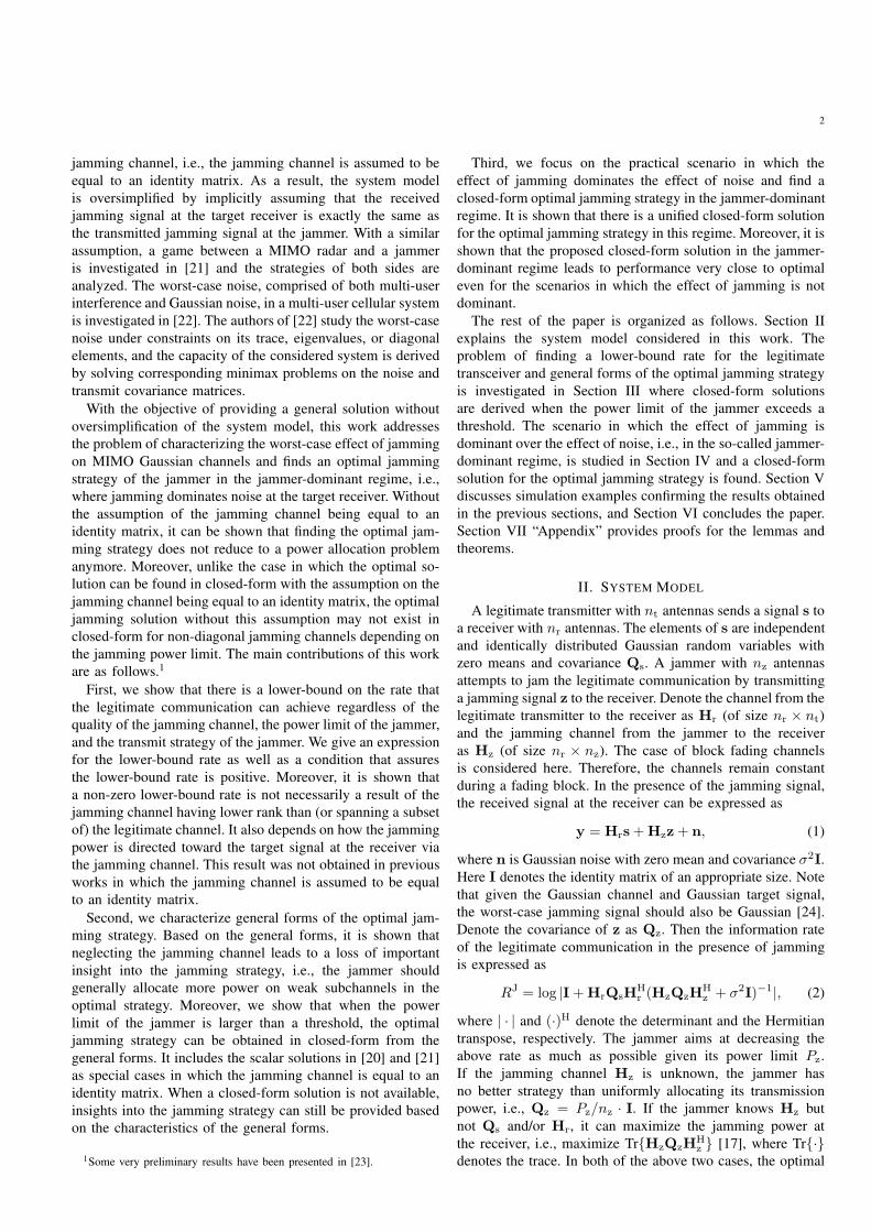
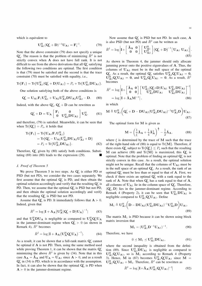
PJD

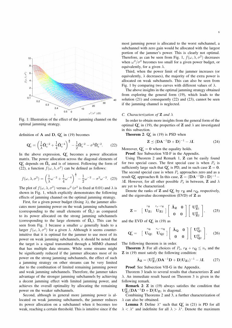
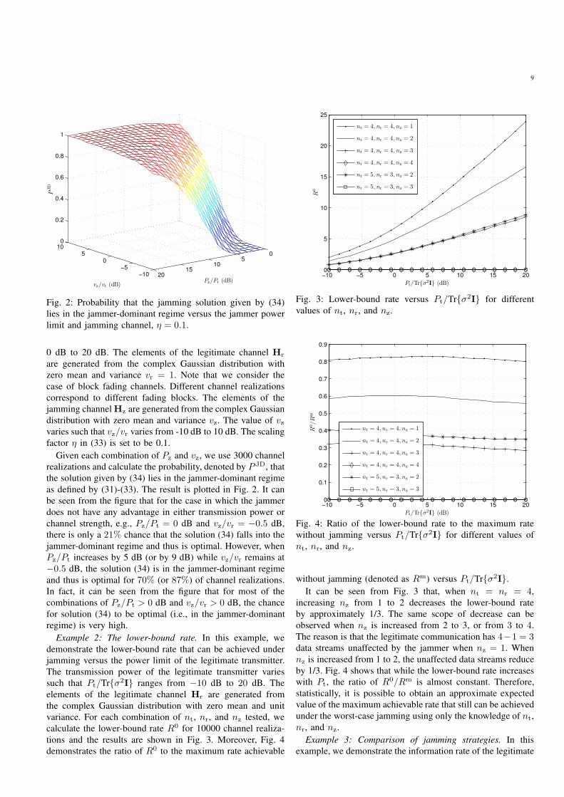
Fig. 2: Probability that the jamming solution given by (34)

lies in the jammer-dominant regime versus the jammer power

limit and jamming channel, η = 0.1.

0 dB to 20 dB. The elements of the legitimate channel Hr

are generated from the complex Gaussian distribution with

zero mean and variance vr = 1. Note that we consider the

case of block fading channels. Different channel realizations

correspond to different fading blocks. The elements of the

jamming channel Hz are generated from the complex Gaussian

distribution with zero mean and variance vz. The value of vzvaries such that vz/vr varies from -10 dB to 10 dB. The scaling

factor η in (33) is set to be 0.1.

Given each combination of Pz and vz, we use 3000 channel

realizations and calculate the probability, denoted by P JD, that

the solution given by (34) lies in the jammer-dominant regime

as defined by (31)-(33). The result is plotted in Fig. 2. It can

be seen from the figure that for the case in which the jammer

does not have any advantage in either transmission power or

channel strength, e.g., Pz/Pt = 0 dB and vz/vr = −0.5 dB,

there is only a 21% chance that the solution (34) falls into the

jammer-dominant regime and thus is optimal. However, when

Pz/Pt increases by 5 dB (or by 9 dB) while vz/vr remains at

−0.5 dB, the solution (34) is in the jammer-dominant regime

and thus is optimal for 70% (or 87%) of channel realizations.

In fact, it can be seen from the figure that for most of the

combinations of Pz/Pt > 0 dB and vz/vr > 0 dB, the chance

for solution (34) to be optimal (i.e., in the jammer-dominant

regime) is very high.

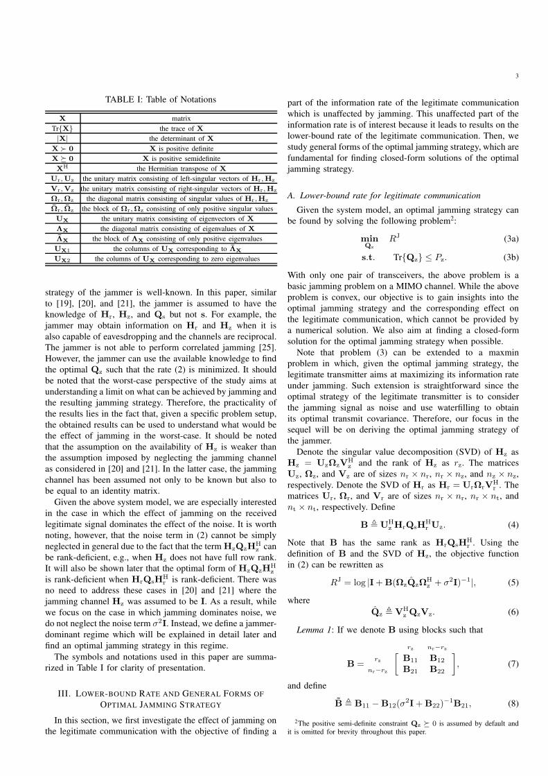
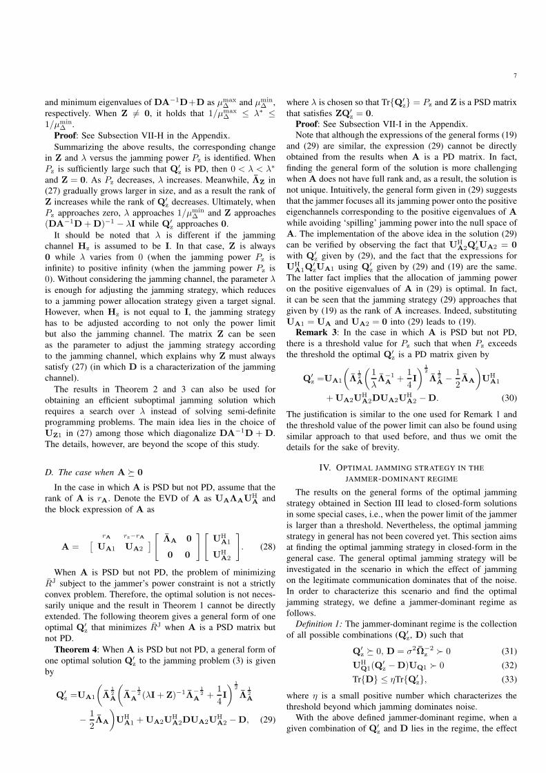
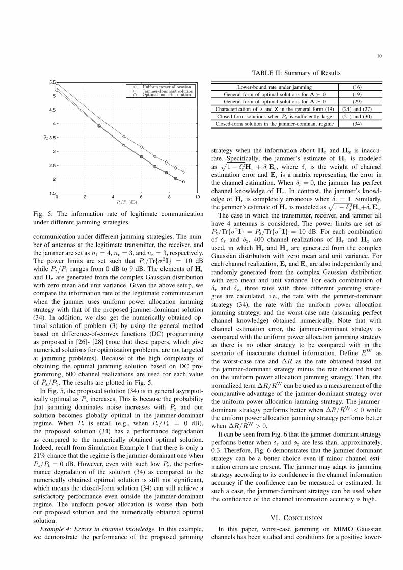
Example 2: The lower-bound rate. In this example, we

demonstrate the lower-bound rate that can be achieved under

jamming versus the power limit of the legitimate transmitter.

The transmission power of the legitimate transmitter varies

such that Pt/Trσ2I ranges from −10 dB to 20 dB. The

elements of the legitimate channel Hr are generated from

the complex Gaussian distribution with zero mean and unit

variance. For each combination of nt, nr, and nz tested, we

calculate the lower-bound rate R0 for 10000 channel realiza-

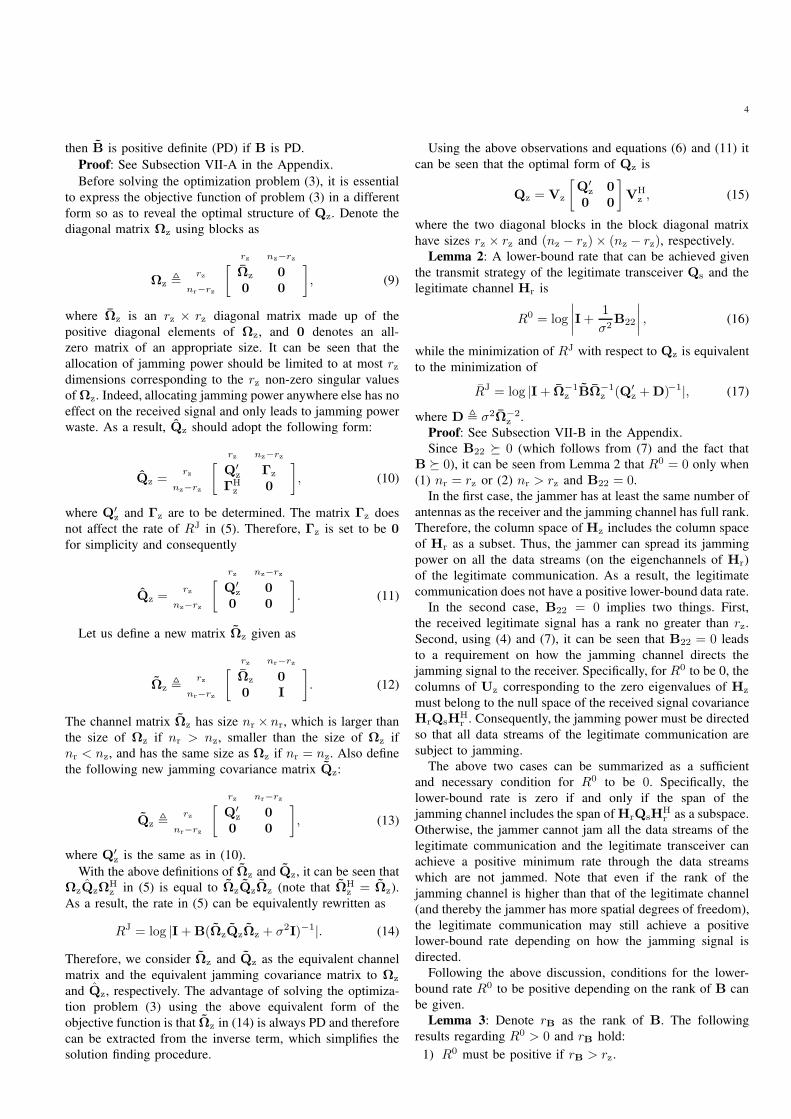
tions and the results are shown in Fig. 3. Moreover, Fig. 4

demonstrates the ratio of R0 to the maximum rate achievable

−10 −5 0 5 10 15 200

5

10

15

20

25

Pt/Trσ2I (dB)

R0

nt = 4, nr = 4, nz = 1

nt = 4, nr = 4, nz = 2

nt = 4, nr = 4, nz = 3

nt = 4, nr = 4, nz = 4

nt = 5, nr = 3, nz = 2

nt = 5, nr = 3, nz = 3

Fig. 3: Lower-bound rate versus Pt/Trσ2I for different

values of nt, nr, and nz.

−10 −5 0 5 10 15 200

0.1

0.2

0.3

0.4

0.5

0.6

0.7

0.8

0.9

Pt/Trσ2I (dB)

R0/R

m

nt = 4, nr = 4, nz = 1

nt = 4, nr = 4, nz = 2

nt = 4, nr = 4, nz = 3

nt = 4, nr = 4, nz = 4

nt = 5, nr = 3, nz = 2

nt = 5, nr = 3, nz = 3

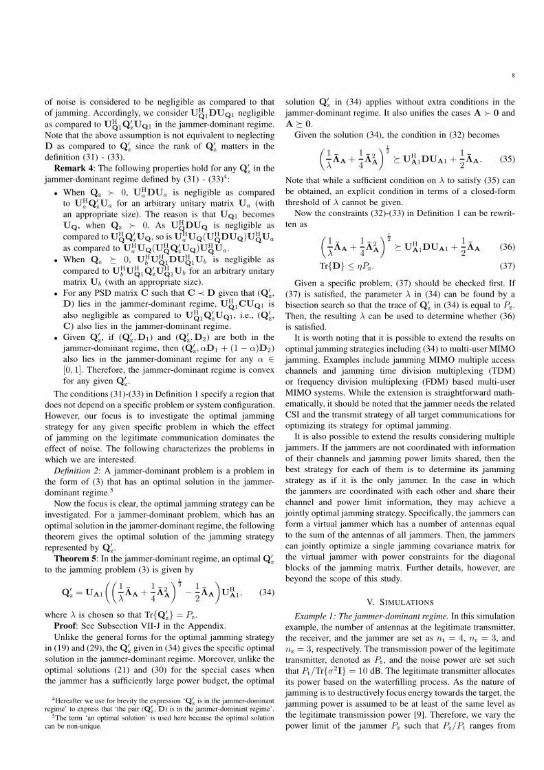
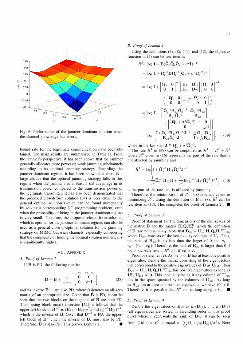
Fig. 4: Ratio of the lower-bound rate to the maximum rate

without jamming versus Pt/Trσ2I for different values of

nt, nr, and nz.

without jamming (denoted as Rm) versus Pt/Trσ2I.

It can be seen from Fig. 3 that, when nt = nr = 4,

increasing nz from 1 to 2 decreases the lower-bound rate

by approximately 1/3. The same scope of decrease can be

observed when nz is increased from 2 to 3, or from 3 to 4.

The reason is that the legitimate communication has 4−1 = 3data streams unaffected by the jammer when nz = 1. When

nz is increased from 1 to 2, the unaffected data streams reduce

by 1/3. Fig. 4 shows that while the lower-bound rate increases

with Pt, the ratio of R0/Rm is almost constant. Therefore,

statistically, it is possible to obtain an approximate expected

value of the maximum achievable rate that still can be achieved

under the worst-case jamming using only the knowledge of nt,

nr, and nz.

Example 3: Comparison of jamming strategies. In this

example, we demonstrate the information rate of the legitimate

10

0 2 4 6 8 101.5

2

2.5

3

3.5

4

4.5

5

5.5

Pz/Pt (dB)

RJ

Uniform power allocationJammer-dominant solutionOptimal numeric solution

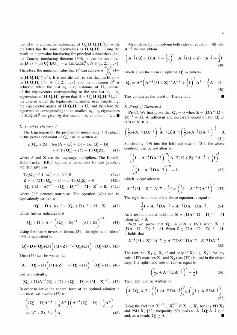
Fig. 5: The information rate of legitimate communication

under different jamming strategies.

communication under different jamming strategies. The num-

ber of antennas at the legitimate transmitter, the receiver, and

the jammer are set as nt = 4, nr = 3, and nz = 3, respectively.

The power limits are set such that Pt/Trσ2I = 10 dB

while Pz/Pt ranges from 0 dB to 9 dB. The elements of Hr

and Hz are generated from the complex Gaussian distribution

with zero mean and unit variance. Given the above setup, we

compare the information rate of the legitimate communication

when the jammer uses uniform power allocation jamming

strategy with that of the proposed jammer-dominant solution

(34). In addition, we also get the numerically obtained op-

timal solution of problem (3) by using the general method

based on difference-of-convex functions (DC) programming

as proposed in [26]- [28] (note that these papers, which give

numerical solutions for optimization problems, are not targeted

at jamming problems). Because of the high complexity of

obtaining the optimal jamming solution based on DC pro-

gramming, 600 channel realizations are used for each value

of Pz/Pt. The results are plotted in Fig. 5.

In Fig. 5, the proposed solution (34) is in general asymptot-

ically optimal as Pz increases. This is because the probability

that jamming dominates noise increases with Pz and our

solution becomes globally optimal in the jammer-dominant

regime. When Pz is small (e.g., when Pz/Pt = 0 dB),

the proposed solution (34) has a performance degradation

as compared to the numerically obtained optimal solution.

Indeed, recall from Simulation Example 1 that there is only a

21% chance that the regime is the jammer-dominant one when

Pz/Pt = 0 dB. However, even with such low Pz, the perfor-

mance degradation of the solution (34) as compared to the

numerically obtained optimal solution is still not significant,

which means the closed-form solution (34) can still achieve a

satisfactory performance even outside the jammer-dominant

regime. The uniform power allocation is worse than both

our proposed solution and the numerically obtained optimal

solution.

Example 4: Errors in channel knowledge. In this example,

we demonstrate the performance of the proposed jamming

TABLE II: Summary of Results

Lower-bound rate under jamming (16)

General form of optimal solutions for A ≻ 0 (19)

General form of optimal solutions for A 0 (29)

Characterization of λ and Z in the general form (19) (24) and (27)

Closed-form solutions when Pz is sufficiently large (21) and (30)

Closed-form solution in the jammer-dominant regime (34)

strategy when the information about Hr and Hz is inaccu-

rate. Specifically, the jammer’s estimate of Hr is modeled

as√

1− δ2rHr + δrEr, where δr is the weight of channel

estimation error and Er is a matrix representing the error in

the channel estimation. When δr = 0, the jammer has perfect

channel knowledge of Hr. In contrast, the jammer’s knowl-

edge of Hr is completely erroneous when δr = 1. Similarly,

the jammer’s estimate of Hz is modeled as√

1− δ2zHz+δzEz.

The case in which the transmitter, receiver, and jammer all

have 4 antennas is considered. The power limits are set as

Pt/Trσ2I = Pz/Trσ2I = 10 dB. For each combination

of δr and δz, 400 channel realizations of Hr and Hz are

used, in which Hr and Hz are generated from the complex

Gaussian distribution with zero mean and unit variance. For

each channel realization, Er and Ez are also independently and

randomly generated from the complex Gaussian distribution

with zero mean and unit variance. For each combination of

δr and δz, three rates with three different jamming strate-

gies are calculated, i.e., the rate with the jammer-dominant

strategy (34), the rate with the uniform power allocation

jamming strategy, and the worst-case rate (assuming perfect

channel knowledge) obtained numerically. Note that with

channel estimation error, the jammer-dominant strategy is

compared with the uniform power allocation jamming strategy

as there is no other strategy to be compared with in the

scenario of inaccurate channel information. Define RW as

the worst-case rate and ∆R as the rate obtained based on

the jammer-dominant strategy minus the rate obtained based

on the uniform power allocation jamming strategy. Then, the

normalized term ∆R/RW can be used as a measurement of the

comparative advantage of the jammer-dominant strategy over

the uniform power allocation jamming strategy. The jammer-

dominant strategy performs better when ∆R/RW < 0 while

the uniform power allocation jamming strategy performs better

when ∆R/RW > 0.

It can be seen from Fig. 6 that the jammer-dominant strategy

performs better when δr and δz are less than, approximately,

0.3. Therefore, Fig. 6 demonstrates that the jammer-dominant

strategy can be a better choice even if minor channel esti-

mation errors are present. The jammer may adapt its jamming

strategy according to its confidence in the channel information

accuracy if the confidence can be measured or estimated. In

such a case, the jammer-dominant strategy can be used when

the confidence of the channel information accuracy is high.

VI. CONCLUSION

In this paper, worst-case jamming on MIMO Gaussian

channels has been studied and conditions for a positive lower-

11

0

0.5

1

00.2

0.40.6

0.81

−0.1

−0.05

0

0.05

0.1

0.15

0.2

0.25

δrδz

∆R

/R

W

Fig. 6: Performance of the jammer-dominant solution when

the channel knowledge has errors.

bound rate for the legitimate communication have been ob-

tained. The main results are summarized in Table II. From

the jammer’s perspective, it has been shown that the jammer

generally allocates more power on weak jamming subchannels

according to its optimal jamming strategy. Regarding the

jammer-dominant regime, it has been shown that there is a

large chance that the optimal jamming strategy falls in this

regime when the jammer has at least 5 dB advantage in its

transmission power compared to the transmission power of

the legitimate transmitter. It has also been demonstrated that

the proposed closed-form solution (34) is very close to the

general optimal solution (which can be found numerically

by solving a corresponding DC programming problem) even

when the probability of being in the jammer-dominant regime

is very small. Therefore, the proposed closed-form solution,

which is optimal for the jammer-dominant regime, can also be

used as a general close-to-optimal solution for the jamming

strategy on MIMO Gaussian channels, especially considering

that the complexity of finding the optimal solution numerically

is significantly higher.

VII. APPENDIX

A. Proof of Lemma 1

If B is PD, the following matrix:

B = B+

[

rz nr−rz

rz 0 0

nr−rz 0 σ2I

]

(38)

and its inverse B−1 are also PD, where 0 denotes an all-zero

matrix of an appropriate size. Given that B is PD, it can be

seen that the two blocks on the diagonal of B are both PD.

Then, using block matrix inversion [29], it follows that the

upper-left block of B−1 is (B11−B12(σ2I+B22)

−1B21)−1,

which is the inverse of B. Given that B−1 is PD, the upper-

left block of B−1, i.e., the inverse of B, must also be PD.

Therefore, B is also PD. This proves Lemma 1.

B. Proof of Lemma 2

Using the definitions (7), (8), (11), and (12), the objective

function in (5) can be rewritten as

RJ= log |I+B(ΩzQzΩz + σ2I)−1|

= log

∣

∣

∣

∣

∣

I+ Ω−1

z BΩ−1

z (Qz + σ2Ω−2

z )−1

∣

∣

∣

∣

∣

= log

∣

∣

∣

∣

∣

I+

[

Ωz 0

0 I

]

−1[

B11 B12

B21 B22

][

Ωz 0

0 I

]

−1

·

([

Q′

z 0

0 0

]

+ σ2

[

Ω−2z 0

0 I

])

−1∣

∣

∣

∣

∣

= log

∣

∣

∣

∣

I+

[

Ω−1z B11Ωz

−1Ω−1

z B12

B21Ω−1z B22

]

·

[

(Q′

z + σ2Ω−2z )−1 0

0 1

σ2 I

]∣

∣

∣

∣

= log

∣

∣

∣

∣

[

I+Ω−1z B11Ω

−1z J−1 1

σ2 Ω−1z B12

B21Ω−1z J−1 I+ 1

σ2B22

]∣

∣

∣

∣

, (39)

where in the last step J , Q′

z + σ2Ω−2z .

The rate RJ in (39) can be simplified as RJ = R0 + RJ

where R0 given in (16) represents the part of the rate that is

not affected by jamming and

RJ = log

∣

∣

∣

∣

I+ Ω−1

z B11Ω−1

z J−1

−1

σ2Ω−1

z B12(I+1

σ2B22)

−1B21Ω−1

z J−1

∣

∣

∣

∣

(40)

is the part of the rate that is affected by jamming.

Therefore, the minimization of RJ in (3a) is equivalent to

minimizing RJ. Using the definition of B in (8), RJ can be

rewritten as (17). This completes the proof of Lemma 2.

C. Proof of Lemma 3

Proof of statement 1): The dimensions of the null spaces of

the matrix B and the matrix HrQsHHr , given the definition

of B, are both nr − rB. Note that B22 = UHzmHrQsH

Hr Uzm

where Uzm consists of the last nr − rz columns of Uz. Thus,

the rank of B22 is no less than the larger of 0 and nr −rz − (nr − rB). Therefore, the rank of B22 is larger than 0 if

rB > rz. As a result, R0 > 0 if rB > rz.

Proof of statement 2): As rB > 0, B has at least one positive

eigenvalue. Denote the matrix consisting of the eigenvectors

that correspond to the positive eigenvalues of B as UB1. Then

B22 = UHzmHrQsH

Hr Uzm has positive eigenvalues as long as

UHzmUB1 6= 0. This inequality holds if any column of Uzm

lies in the space spanned by the columns of UB1. As long

as B22 has at least one positive eigenvalue, we have R0 > 0.

Therefore, it is possible that R0 > 0 as long as rB > 0.

D. Proof of Lemma 4

Denote the eigenvalues of B22 as µ1(B22), . . . , µr(B22)(all eigenvalues are sorted in ascending order in this proof

only) where r represents the rank of B22. It can be seen

from (16) that R0 is equal tor∑

i=1

(1 + µi(B22)/σ2). Note

12

that B22 is a principal submatrix of UHz HrQsH

Hr Uz while

the latter has the same eigenvalues as HrQsHHr . Using the

result on eigenvalue interlacing for principal submatrices (i.e.,

the Cauchy interlacing theorem [30]), it can be seen that

µi(B22) ≥ µi(UHz BUz) = µi(HrQsH

Hr ), ∀i ∈ 1, 2, . . . , r.

Therefore, the minimum value that R0 can achieve isnr−rz∑

i=1

(1+

µi(HrQsHHr )/σ

2). It is not difficult to see that µi(B22) =µi(HrQsH

Hr ), ∀i ∈ 1, 2, . . . , r and the minimum R0 is

achieved when the last nr − rz columns of Uz consist

of the eigenvectors corresponding to the smallest nr − rzeigenvalues of HrQsH

Hr given that B = UH

z HrQsHHr Uz. In

the case in which the legitimate transmitter uses waterfilling,

the eigenvector matrix of HrQsHHr is Ur and therefore the

eigenvectors corresponding to the smallest nr−rz eigenvalues

of HrQsHHr are given by the last nr − rz columns of Ur.

E. Proof of Theorem 1

The Lagrangian for the problem of minimizing (17) subject

to the power constraint of Q′

z can be written as

L(Q′

z, λ,Z) = log |A+Q′

z +D| − log |Q′

z +D|

+ λ(TrQ′

z − Pz) + TrQ′

zZ, (41)

where λ and Z are the Lagrange multipliers. The Karush-

Kuhn-Tucker (KKT) optimality conditions for this problem

are then given as

TrQ′

z ≤ 1, Q′

z 0, λ ≥ 0 (42a)

Z 0, λ(TrQ′

z − 1) = 0, TrQ′

zZ = 0 (42b)

(Q′

z +D+A)−T − (Q′

z +D)−T + λI+ ZT = 0, (42c)

where (·)T denotes transpose. The equation (42c) can be

equivalently written as

(Q′

z +D+A)−1 = (Q′

z +D)−1 − λI− Z, (43)

which further indicates that

Q′

z +D+A =

(

(Q′

z +D)−1 − (λI + Z)

)

−1

. (44)

Using the matrix inversion lemma [31], the right-hand side of

(44) is equivalent to

Q′

z+D+(Q′

z+D)

(

(λI+Z)−1−(Q′

z+D)

)

−1

(Q′

z+D). (45)

Then (44) can be written as

A = (Q′

z+D)

(

(λI+Z)−1− (Q′

z+D)

)

−1

(Q′

z+D), (46)

and equivalently,

(Q′

z +D)A−1(Q′

z +D) + (Q′

z +D) = (λI+ Z)−1. (47)

In order to derive the general form of the optimal solution in

our case, we rewrite (47) as(

(Q′

z +D)A−1

2 +1

2A

1

2

)(

A−1

2 (Q′

z +D) +1

2A

1

2

)

= (λI+ Z)−1 +1

4A. (48)

Meanwhile, by multiplying both sides of equation (48) with

A−1

2 we can obtain(

A−1

2 (Q′

z +D)A−1

2 +1

2I

)2

= A−1

2 (λI + Z)−1A−1

2 +1

4I,

(49)

which gives the form of optimal Q′

z as follows

Q′

z = A1

2

(

A−1

2 (λI+ Z)−1A−1

2 +1

4I

)1

2

A1

2 −1

2A−D.

(50)

This completes the proof of Theorem 1.

F. Proof of Theorem 2

Proof: We first prove that Q′

z = 0 when Z = (DA−1D+D)−1 − λI. A sufficient and necessary condition for Q′

z in

(19) to be 0 is

(

1

2I+A−

1

2DA−1

2

)

−1

2

A−1

2Q′

zA−

1

2

(

1

2I+A−

1

2DA−1

2

)

−1

2

= 0.

(51)

Substituting (19) into the left-hand side of (51), the above

condition can be rewritten as(

1

2I+A−

1

2DA−1

2

)

−1

2

(

A−1

2 (λI+ Z)−1A−1

2 +1

4I

)1

2

·

(

1

2I+A−

1

2DA−1

2

)

−1

2

= I, (52)

which is equivalent to

A−1

2 (λI + Z)−1A−1

2 +1

4I =

(

1

2I+A−

1

2DA−1

2

)2

. (53)

The right-hand side of the above equation is equal to

1

4I+A−

1

2DA−1

2 +A−1

2DA−1DA−1

2 . (54)

As a result, it must hold that Z = (DA−1D + D)−1 − λIwhen Q′

z = 0.

Next we prove that Q′

z in (19) is PSD when Z (DA−1D+D)−1 − λI. When Z (DA−1D+D)−1 − λI,it holds that

A−1

2 (λI+ Z)−1A−1

2 A−1

2DA−1DA−1

2 +A−1

2DA−1

2 .(55)

The fact that X1 X2 if and only if X−1

2 X−1

1for any

pair of PD matrices X1 and X2 (see [32]) is used in the above

step. The right-hand side of (55) is equal to(

1

2I+A−

1

2DA−1

2

)2

−1

4I. (56)

Then, (55) can be written as(

A−1

2Q′

zA−

1

2 +

(

1

2I+A−

1

2DA−1

2

))2

(

1

2I+A−

1

2DA−1

2

)2

.

(57)

Using the fact that X1/21

X1/22

if X1 X2 for any PD X1

and PSD X2 [32], inequality (57) leads to A−1

2Q′

zA−

1

2 0and, as a result, Q′

z 0.

13

G. Proof of Theorem 3

Proof: The constraint TrQ′

zZ = 0 in (42b) indicates

that TrQ′

z

1

2 (−Z)Q′

z

1

2 = 0. As −Z and Q′

z are both PSD,

Q′

z

1

2 (−Z)Q′

z

1

2 must be PSD. Therefore, the trace constraint

implies that Q′

z

1

2ZQ′

z

1

2 = 0. Consequently, it can be shown

that

UH

Z1Q′

zUZ1 = UH

Z1UQ1ΛQUH

Q1UZ1 = 0. (58)

As a result, Z and Q′

z satisfy the condition

ZQ′

z = Q′

zZ = 0. (59)

It can be seen that rZ + rQ ≤ nz from the above equations.

Then, we can obtain the following result from equation (47)

Z(Q′

z+D)A−1(Q′

z+D)Z+Z(Q′

z+D)Z = Z(λI+Z)−1Z.(60)

Using the property that ZQ′

z = Q′

zZ = 0, (60) simplifies to

ZDA−1DZ+ ZDZ = Z(λI + Z)−1Z. (61)

Define N , DA−1D+D and note that N is PD. The above

equation (61) can be rewritten as

Z(

N− (λI − Z)−1)

Z = 0. (62)

Using (25), equation (62) can be rewritten as

[

ΛZ 0

0 0

]

(

N−

(

λI+

[

ΛZ 0

0 0

])

−1)

[

ΛZ 0

0 0

]

= 0,

(63)

where

N =

[

UHZ1

UHZ2

]

N[

UZ1 UZ2

]

. (64)

From (63) and (64), the following result can be obtained:

UH

Z1NUZ1 − (λI+ΛZ)−1 = 0, (65)

or equivalently,

ΛZ = (UH

Z1NUZ1)−1 − λI. (66)

Substituting N back into (66) completes the proof.

H. Proof of Lemma 5

Proof: Using (27) in Theorem 3, it can be seen that Z 0

whenever λ < 1/µmax∆

, which contradicts the constraint Z 0

in (42b). Therefore, λ∗ ≥ 1/µmax∆

. According to Theorem 2,

at the point when λ becomes as small as 1/µmin∆

(the same

point when (DA−1D + D)−1 − λI becomes negative semi-

definite), Z = (DA−1D + D)−1 − λI leads to the result

Q′

z = 0. Therefore, λ∗ ≤ 1/µmin∆

.

I. Proof of Theorem 4

Given the block representation of A in (28), the RJ in (17)

can be rewritten as

RJ = log

∣

∣

∣

∣

I+[

UA1 UA2

]

[

ΛA 0

0 0

] [

UHA1

UHA2

]

Q′′

z

−1

∣

∣

∣

∣

= log

∣

∣

∣

∣

∣

I+

[

ΛA 0

0 0

]([

UHA1

UHA2

]

Q′′

z

[

UA1 UA2

]

)

−1∣

∣

∣

∣

∣

= log

∣

∣

∣

∣

∣

I+

[

ΛA 0

0 0

] [

UHA1

Q′′

zUA1 UHA1

Q′′

zUA2

UHA2

Q′′

zUA1 UHA2

Q′′

zUA2

]

−1∣

∣

∣

∣

∣

= log

∣

∣

∣

∣

I+ ΛAF−1

1

∣

∣

∣

∣

, (67)

where Q′′

z , Q′

z+D, and the result on block matrix inversion

[29] is used in the last equality, in which

F1 , UH

A1

(

Q′′

z −Q′′

zUA2(UH

A2Q′′

zUA2)−1UH

A2Q′′

z

)

UA1.

(68)

Since ΛA in (67) is PD, the result (19) can be used here.

Applying the result (19), the optimal F1 is given by

F1 = Λ1

2

A

(

Λ−

1

2

A (λI+ Z)Λ−

1

2

A +1

4I

)1

2

Λ1

2

A −1

2ΛA. (69)

It should be noted that the variable λ is determined by the

trace of F1, which satisfies

TrF1 ≤ TrUH

A1(Q′

z +D)UA1 ≤ Pz + TrUH

A1DUA1.(70)

Considering the fact that

UH

A2

(

Q′′

z−Q′′

zUA2(UH

A2Q′′

zUA2)−1UH

A2Q′′

z

)

UA2=0 (71)

UH

A1

(

Q′′

z−Q′′

zUA2(UH

A2Q′′

zUA2)−1UH

A2Q′′

z

)

UA2=0 (72)

UH

A2

(

Q′′

z−Q′′

zUA2(UH

A2Q′′

zUA2)−1UH

A2Q′′

z

)

UA1=0, (73)

it leads to the following result

Q′′

z −Q′′

zUA2(UH

A2Q′′

zUA2)−1UH

A2Q′′

z = UA1F1UH

A1.(74)

The equation (74) can be further rewritten as

Q′′

z

−1−UA2(U

H

A2Q′′

zUA2)−1UH

A2

= Q′′

z

−1UA1F1U

H

A1Q′′

z

−1, (75)

which implies that

UH

A1Q′′

z

−1UA1 = UH

A1Q′′

z

−1UA1F1U

H

A1Q′′

z

−1UA1. (76)

As a result, it holds that

UH

A1Q′′

z

−1UA1(F1U

H

A1Q′′

z

−1UA1 − I) = 0. (77)

Since F1 and Q′′

z are both PD matrices, Q′′

z must satisfy

UH

A1Q′′

z

−1UA1 = F−1

1, (78)

14

which is equivalent to

UH

A1(Q′

z +D)−1UA1 = F−1

1. (79)

Note that the above constraint (79) does not specify a unique

Q′

z. The reason is that the problem of minimizing RJ is not

strictly convex when A does not have full rank. It is not

difficult to see from the above derivations that all Q′

z satisfying

the following two conditions are optimal. The first condition

is that (79) must be satisfied and the second is that the trace

constraint (70) must be satisfied with equality, i.e.,

TrF1 = TrUH

A1(Q′

z +D)UA1 = Pz + TrUH

A1DUA1.

One solution satisfying both of the above conditions is

Q′

z = UA1F1UH

A1 +UA2UH

A2DUA2UH

A2 −D. (80)

Indeed, with the above Q′

z, Q′

z +D can be rewritten as

Q′

z +D = UA

[

F1 0

0 UH

A2DUA2

]

UH

A, (81)

and therefore, (79) is satisfied. Meanwhile, it can be seen that

when TrQ′

z = Pz, it holds that

TrF1 = TrUA1F1UH

A1

= TrQ′

z −UA2UH

A2DUA2UH

A2 +D

= Pz + TrUH

A1DUA1. (82)

Therefore, Q′

z given by (80) satisfy both conditions. Substi-

tuting (69) into (80) leads to the expression (29).

J. Proof of Theorem 5

We prove Theorem 5 in two steps. As Q′

z is either PD or

PSD (but not PD), we consider the two cases separately. We

first assume that the optimal Q′

z is PD, and then obtain the

optimal solution accordingly and verify that the resulting Q′

z is

PD. Then, we assume that the optimal Q′

z is PSD but not PD,

and then obtain the optimal solution accordingly and verify

that the resulting Q′

z is PSD but not PD.

Assume that Q′

z is PD. It immediately follows that A ≻ 0.

Indeed, given that

RJ = log |I+ΛA

(

UH

A(Q′

z +D)UA

)

−1| (83)

and that UH

ADUA is negligible as compared to UH

AQ′

zUA

in the jammer-dominant regime when Q′

z ≻ 0 (as shown in

Remark 4), RJ becomes

RJ = log |I+ΛA

(

UH

AQ′

zUA

)

−1|. (84)

As a result, it can be shown that a full-rank matrix Q′

z cannot

be optimal if A is not PD. Then, using the same method used

while proving Theorem 1, it can be shown that the matrix Q′

z

minimizing the above RJ is given by (34). Note that in this

case ΛA = ΛA and UA = UA1 since A ≻ 0, and as a result

Q′

z in (34) is PD, which is in accordance with the assumption.

In fact, it can also be shown that the optimal Q′

z is PD when

A ≻ 0 in the jammer-dominant regime.

Now assume that Q′

z is PSD but not PD. In such case, A

is also PSD (but not PD) and RJ can be written as

RJ = log

∣

∣

∣

∣

I+

[

ΛA 0

0 0

] [

UHA1

UHA2

]

(

Q′

z +D)

−1[

UA1 UA2

]

∣

∣

∣

∣

.

(85)

As shown in Theorem 4, the jammer should only allocate

jamming power onto the positive eigenvalues of A. Thus, the

columns of UA2 must be in the null space of the optimal

Q′

z. As a result, the optimal Q′

z satisfies UHA2

Q′

zUA2 = 0,

UHA1

Q′

zUA2 = 0, and UHA2

Q′

zUA1 = 0. As a result, RJ

becomes

RJ = log

∣

∣

∣

∣

∣

I+

[

ΛA 0

0 0

] [

UHA1

(Q′

z+D)UA1 UHA1

DUA2

UHA2

DUA1 UHA2

DUA1

]

−1∣

∣

∣

∣

∣

= log∣

∣I+ ΛAM−1∣

∣ , (86)

in which

M , UH

A1

(

Q′

z +D−DUA2(UH

A2DUA2)−1UH

A2D

)

UA1.

(87)

The optimal form for M is given as

M =

(

1

ξΛA +

1

4Λ2

A

)1

2

−1

2ΛA, (88)

where ξ is determined by the trace of M such that the trace

of the right-hand side of (88) is equal to TrM. Therefore, if

there exists Q′

z subject to TrQ′

z ≤ Pz such that the resulting

M can achieve (88) and TrM is maximized, this Q′

z is

optimal. Note that the problem of finding an optimal Q′

z is not

strictly convex in this case. As a result, the optimal solution

might not be unique. Recall that the columns of UA2 must be

in the null space of an optimal Q′

z. As a result, the rank of an

optimal Q′

z must be less than or equal to that of A. First, we

check if there exists an optimal Q′

z with a rank equal to the

rank of A. Note that when Q′

z has a rank equal to that of A,

all columns of UA1 lie in the column space of Q′

z. Therefore,

(Q′

z,D) lies in the jammer-dominant regime. According to

Remark 4 (Property 2), it can be seen that UHA1

DUA1 is

negligible compared to UHA1

Q′

zUA1. Define

M1 , UH

A1

(

D−DUA2(UH

A2DUA2)−1UH

A2D

)

UA1.

(89)

The matrix M1 is PSD because it can be shown using block

matrix inversion that

M1 = (UH

A1D−1UA1)

−1. (90)

Therefore, we have

0 M1 UH

A1DUA1, (91)

where the second inequality is obtained from the defini-

tion (89). Since UHA1

DUA1 is negligible as compared to

UHA1

Q′

zUA1, so is M1 according to Remark 4 (Property

3). Hence, M in (87) becomes UHA1

Q′

zUA1 since M =UH

A1Q′

zUA1 +M1. Therefore, RJ can be rewritten as

RJ = log∣

∣I+ΛA(UH

A1Q′

zUA1)−1∣

∣ (92)

15

and the solution is (34). It can be seen that the solution of

Q′

z in (34) leads to M in (88) as M becomes UHA1

Q′

zUA1 in

the jammer-dominant regime. Q′

z in (34) also maximizes the

trace of M in (87). Moreover, Q′

z in (34) has the same rank

as A as we assumed. Therefore, (34) is an optimal solution

when Q′

z is PSD but not PD.

Combining the above two parts completes the proof of

Theorem 5.

ACKNOWLEDGEMENT

The authors would like to thank the editor Prof. Gesualdo

Scutari and the anonymous reviewers for their valuable com-

ments which helped to improve the quality and clarity of this

manuscript.

REFERENCES

[1] X. Lin, R. Lu, C. Zhang, H. Zhu, P.-H. Ho, and X. Shen, “Securityin vehicular ad hoc networks,” IEEE Commun. Mag., vol. 46, no. 4,pp. 88-95, Apr. 2008.

[2] C. Popper, M. Strasser, and S. Capkun, “Anti-jamming broadcast com-munication using uncoordinated spread spectrum techniques,” IEEE J.

Sel. Areas Commun., vol. 28, no. 5, pp. 703-715, June 2010.[3] A. Chorti, S. M. Perlaza, Z. Han, and H. V. Poor, “On the resilience of

wireless multiuser networks to passive and active eavesdroppers,” IEEE

J. Sel. Areas Commun., vol. 31, no. 9, pp. 1850-1863, Sept. 2013.[4] E. Bou-Harb, C. Fachkha, M. Pourzandi, M. Debbabi, and C. Assi,

“Communication security for smart grid distribution networks,” IEEE

Commun. Mag., vol. 51, no. 1, pp. 42-49, Jan. 2013.[5] Y.-S. Shiu, S. Y. Chang, H.-C. Wu, S. C.-H. Huang, and H.-H. Chen,

“Physical layer security in wireless networks: A tutorial,” IEEE WirelessCommun., vol. 18, no. 2, pp. 66-74, Apr. 2011.

[6] W. Xu, W. Trappe, Y. Zhang, and T. Wood, “The feasibility of launchingand detecting jamming attacks in wireless networks,” in Proc. ACM

Int. Symp. Mobile Ad Hoc Netw. and Comput. (MobiHoc), Urbana-Champaign, IL, USA, May 2005, pp. 46-57.

[7] R. A. Poisel, Modern Communications Jamming: Principles and Tech-

niques, Artech House, 2nd Ed., 2011.[8] M. Li, I. Koutsopoulos, and R. Poovendran, “Optimal jamming attack

strategies and network defense policies in wireless sensor networks,”IEEE Trans. Mobile Comput., vol. 9, no. 8, pp. 1119-1133, Aug. 2010.

[9] Q. Peng, P. C. Cosman, and L. B. Milstein, “Spoofing or jamming:Performance analysis of a tactical cognitive radio adversary,” IEEE J.

Sel. Areas Commun., vol. 29, no. 4, pp. 903-911, Apr. 2011.[10] S. Sodagari and T. C. Clancy, “Efficient jamming attacks on MIMO

channels,” in Proc. IEEE Int. Conf. Commun., Ottawa, Canada, June2012, pp. 852-856.

[11] S. Wei and R. Kannan, “Jamming and counter-measure strategies inparallel Gaussian fading channels with channel state information,” inProc. IEEE Military Commun. Conf., San Diego, USA, Nov. 2008, pp. 1-7.

[12] D. J. Torrieri, “Fundamental limitations on repeater jamming offrequency-hopping communications,” IEEE J. Sel. Areas Commun.,vol. 7, no. 4, pp. 569-575, May 1989.

[13] S. Prasad and D. J. Thuente, “Jamming attacks in 802.11g: A cognitiveradio based approach,” in Proc. IEEE Military Commun. Conf., Balti-more, USA, Nov. 2011, pp. 1219-1224.

[14] A. A. Ali, “Worst-case partial-band noise jamming of Rician fadingchannels,” IEEE Trans. Commun., vol. 44, no. 6, pp. 660-662, June1996.

[15] M. Soysa, P. C. Cosman, and L. B. Milstein, “Optimized spoofing andjamming a cognitive radio,” IEEE Trans. Commun., vol. 62, no. 8,pp. 2681-2695, Aug. 2014.

[16] H. M. Kwon and P. Lee, “Combined tone and noise jamming againstcoded FH/MFSK ECCM radios,” IEEE J. Sel. Area Commun., vol. 8,no. 5, pp. 871-883, June 1990.

[17] A. Bayesteh, M. Ansari, and A. K. Khandani, “Effect of jamming on thecapacity of MIMO channels”, in Proc. Allerton Conf. Commun. Control

and Comput., Sept.-Oct. 2004, Monticello, USA, pp. 401-410.[18] E. A. Jorswieck, H. Boche, and M. Weckerle, “Optimal transmitter and

jamming strategies in Gaussian MIMO channels,” in Proc. IEEE Veh.

Tech. Conf., Stockholm, Sweden, May-June 2005, pp. 978-982.

[19] M. H. Brady, M. Mohseni, and J. M. Cioffi, “Spatially-correlatedjamming in Gaussian multiple access and broadcast channels,” in Proc.

40th Annu. Conf. Info. Sci. and Syst., Princeton, NJ, USA, Mar. 2006,pp. 1635-1639.

[20] M. R. D. Rodrigues and G. Ramos, “On multiple-input multiple-outputGaussian channels with arbitrary inputs subject to jamming,” in Proc.

IEEE Int. Symp. Info. Theory, Seoul, Korea, June-July 2009, pp. 2512-2516.

[21] X. Song, P. Willett, S. Zhou, and P. B. Luh, “The MIMO radar andjammer games,” IEEE Trans. Signal Processing, vol. 60, no. 2, pp. 687-699, Feb. 2012.

[22] E. A. Jorswieck and H. Boche, “Performance analysis of capacity ofMIMO systems under multiuser interference based on worst-case noisebehavior,” EURASIP J. on Wireless Commun. and Networking, vol. 2,pp. 273-285, 2004.

[23] J. Gao, S. A. Vorobyov, and H. Jiang, “Efficient jamming strategies on aMIMO Gaussian channel with known target signal covariance,” in Proc.

IEEE Int. Conf. Acoustics, Speech, and Signal Processing, Florence,Italy, May 2014, pp. 5700-5704.

[24] S. N. Diggavi, and T. M. Cover, “The worst additive noise undera covariance constraint,” IEEE Trans. Info. Theory, vol. 47, no. 7,pp. 3072-3081, Nov. 2001.

[25] A. Kashyap, T. Basar, and R. Srikant, “Correlated jamming on MIMOGaussian fading channels,” IEEE Trans. Information Theory, vol. 50,no. 9, pp. 2119-2123, Sept. 2004.

[26] K. T. Phan, S. A. Vorobyov, C. Tellambura, and T. Le-Ngoc, “Powercontrol for wireless cellular systems via D.C. programming,” in Proc.

IEEE Workshop Stat. Signal Process., Madison, USA, Aug. 2007,pp. 507-511.

[27] A. Beck, A. Ben-Tal, and L. Tetruashvili, “A sequential parametricconvex approximation method with applications to nonconvex trusstopology design problems,” J. Global Optimization, vol. 47, no. 1,pp. 29-51, May 2010.

[28] A. Khabbazibasmenj, F. Roemer, S. A. Vorobyov, and M. Haardt, “Sum-rate maximization in two-way AF MIMO relaying: Polynomial timesolutions to a class of DC programming problems,” IEEE Trans. SignalProcess., vol. 60, no. 10, pp. 5478-5493, Oct. 2012.

[29] H. Lutkepohl, Handbook of Matrices. John Wiley & Sons, 1997.[30] F. Zhang, Matrix Theory: Basic Results and Techniques. Springer

Science & Business Media, 2011.[31] F. A. Dietrich, Robust Signal Processing for Wireless Communications.

Springer, 2008.[32] R. A. Horn and C. R. Johnson, Matrix Analysis. 2nd Edition. Cambridge

University Press, 2012.

Jie Gao received the B.Eng. degree in electronicsand information engineering from Huazhong Uni-versity of Science and Technology, Wuhan, China,in 2007, and the M.Sc. and Ph.D. degrees in elec-trical engineering from the University of Alberta,Edmonton, Alberta, Canada, in 2009 and 2014,respectively. He is currently a postdoctoral fellowwith the Advanced Wireless Communications andSignal Processing Lab, Department of Electrical &Computer Engineering, and the Centre for SmartTransportation, Department of Civil and Environ-

mental Engineering, at the University of Alberta. His research interests includesignal processing for MIMO communications and cooperative multiusercommunications.

16

Sergiy A. Vorobyov (M’02-SM’05) received theM.Sc. and Ph.D. degrees in systems and control fromKharkiv National University of Radio Electronics,Ukraine, in 1994 and 1997, respectively.

He is a Professor with the Department of SignalProcessing and Acoustics, Aalto University, Finland.He has been previously with the University of Al-berta, Alberta, Canada as an Assistant Professorfrom 2006 to 2010, Associate Professor from 2010to 2012, and became Full Professor there in 2012.Since his graduation, he also held various research

and faculty positions at Kharkiv National University of Radio Electronics,Ukraine; the Institute of Physical and Chemical Research (RIKEN), Japan;McMaster University, Canada; Duisburg-Essen University and DarmstadtUniversity of Technology, Germany; and the Joint Research Institute betweenHeriot-Watt University and Edinburgh University, U.K. He has also held short-term visiting positions at Technion, Haifa, Israel and Ilmenau University ofTechnology, Ilmenau, Germany. His research interests include statistical andarray signal processing; optimization and liner algebra methods in signalprocessing, communications, and machine learning; sparse signal processing;estimation and detection theory; sampling theory; and multi-antenna, cooper-ative, and cognitive systems.

Dr. Vorobyov is a recipient of the 2004 IEEE Signal Processing Society BestPaper Award, the 2007 Alberta Ingenuity New Faculty Award, the 2011 CarlZeiss Award (Germany), the 2012 NSERC Discovery Accelerator Award, andother awards. He served as an Associate Editor for the IEEE Transactionson Signal Processing from 2006 to 2010 and for the IEEE Transactionson Signal Processing Letters from 2007 to 2009. He was a member of theSensor Array and Multi-Channel Signal Processing Committee of the IEEESignal Processing Society from 2007 to 2012. He is a member of the SignalProcessing for Communications and Networking Committee since 2010. Hehas served as the Track Chair for Asilomar 2011, Pacific Grove, CA, theTechnical Co-Chair for IEEE CAMSAP 2011, Puerto Rico, and the TutorialChair for ISWCS 2013, Ilmenau, Germany.

Hai Jiang (SM’15) received the B.Sc. and M.Sc.degrees in electronics engineering from Peking Uni-versity, Beijing, China, in 1995 and 1998, respec-tively, and the Ph.D. degree (with an OutstandingAchievement in Graduate Studies Award) in elec-trical engineering from the University of Waterloo,Waterloo, Ontario, Canada, in 2006.

Since July 2007, he has been a faculty memberwith the University of Alberta, Edmonton, Alberta,Canada, where he is currently a Professor at theDepartment of Electrical & Computer Engineering.

His research interests include radio resource management, cognitive radionetworking, and cooperative communications.

Dr. Jiang is an Editor for the IEEE TRANSACTIONS ON VEHICULARTECHNOLOGY and IEEE WIRELESS COMMUNICATIONS LETTERS.

H. Vincent Poor (S’72, M’77, SM’82, F’87) re-ceived the Ph.D. degree in EECS from PrincetonUniversity in 1977. From 1977 until 1990, he wason the faculty of the University of Illinois at Urbana-Champaign. Since 1990 he has been on the facultyat Princeton, where he is the Michael Henry StraterUniversity Professor of Electrical Engineering andDean of the School of Engineering and AppliedScience. Dr. Poor’s research interests are in the areasof stochastic analysis, statistical signal processing,and information theory, and their applications in

wireless networks and related fields such as social networks and smart grid.Among his publications in these areas is the recent book Mechanisms andGames for Dynamic Spectrum Allocation (Cambridge University Press, 2014).

Dr. Poor is a member of the National Academy of Engineering and theNational Academy of Sciences, and a foreign member of Academia Europaeaand the Royal Society. He is also a fellow of the American Academy ofArts and Sciences, the Royal Academy of Engineering (U. K.), and theRoyal Society of Edinburgh. He received the Technical Achievement andSociety Awards of the IEEE Signal Processing Society in 2007 and 2011,respectively. Recent recognition of his work includes the 2014 URSI BookerGold Medal, and honorary doctorates from several universities in Europe andAsia, including an honorary D.Sc. from Aalto University in 2014.