NBER WORKING PAPER SERIES

WORKER SORTING, COMPENSATING DIFFERENTIALS AND HEALTH INSURANCE:EVIDENCE FROM DISPLACED WORKERS

Steven F. LehrerNuno Sousa Pereira

Working Paper 12951http://www.nber.org/papers/w12951

NATIONAL BUREAU OF ECONOMIC RESEARCH1050 Massachusetts Avenue

Cambridge, MA 02138March 2007

We are grateful to one anonymous referee, Daniel Parent and seminar participants at the 2003 iHEAConference and Fudan University for helpful comments and suggestions that have substantially improvedthe paper. We would also like to thank Kosali Simon for providing code that helped to generate a portionof the dataset used in this study. Lehrer wishes to thank SSHRC for research support. Pereira gratefullyacknowledges support from CETE. CETE, Research Center on Industrial, Labour and ManagerialEconomics, is supported by the Fundacao para a Ciencia e a Tecnologia, Programa de FinanciamentoPlurianual, through the Programa Operacional Ciencia, Tecnologia e Inovacao (POCTI) of the QuadroComunitario de Apoio III, which is financed by FEDER and Portuguese funds. The usual caveat applies.The views expressed herein are those of the author(s) and do not necessarily reflect the views of theNational Bureau of Economic Research.

© 2007 by Steven F. Lehrer and Nuno Sousa Pereira. All rights reserved. Short sections of text, notto exceed two paragraphs, may be quoted without explicit permission provided that full credit, including© notice, is given to the source.

Worker Sorting, Compensating Differentials and Health Insurance: Evidence from DisplacedWorkersSteven F. Lehrer and Nuno Sousa PereiraNBER Working Paper No. 12951March 2007JEL No. I11,J30

ABSTRACT

This article introduces an empirical strategy to the compensating differentials literature that i) allowsboth individual observed and unobserved characteristics to be rewarded differently in firms basedon health insurance provision, and ii) selection to jobs that provide benefits to operate on both sidesof the labor market. Estimates of this model are used to directly test empirical assumptions that aremade with popular econometric strategies in the health economics literature. Our estimates reject theassumptions underlying numerous cross sectional and longitudinal estimators. We find that the provisionof health insurance has influenced wage inequality. Finally, our results suggest there have been substantialchanges in how displaced workers sort to firms that offer health insurance benefits over the past twodecades. We discuss the implications of our findings for the compensating differentials literature.

Steven F. LehrerSchool of Policy Studiesand Department of EconomicsQueen's UniversityKingston, OntarioK7L, 3N6 CANADAand NBERlehrers@post.queensu.ca

Nuno Sousa PereiraDepartment of Economics, University of PortoRua Dr. Roberto Frias4200-464 Porto, Portugalnpereira@fep.up.pt

1 Introduction

Without a national health insurance system most Americans receive health benefits from

their employers. As recent years have been characterized by rapid inflation in health care

costs and health insurance premiums,1 there are increasing reports that employers have

either reduced or even stopped offering coverage, increasing the ranks of the uninsured.2

In aggregate, the percentage of workers with employment-based health insurance has

dropped from 70.0% in 1987 to 59.8% in 2004.

Economists generally argue that profit maximizing employers would respond to the

costs associated with the provision of health insurance by reducing wages, thus maintain-

ing the total reward paid to the employees. Whether employers truly adjust wages for

the provision of health insurance is a long-standing question in health economics. Evi-

dence of a wage / fringe benefit tradeoff has been difficult to establish empirically, in part

because jobs that offer health insurance may differ substantially from those where this

benefit is not provided.3 Empirical researchers have traditionally attempted to answer

this question using wage regressions. Researchers arrive at conclusions by examining the

sign and significance of the estimated coefficient on the health insurance receipt variable.

Studies generally differ in the source of variation used to identify health insurance receipt

in these regressions. The early literature on this topic typically did not explicitly contain

a discussion of the source of variation in the health insurance variable and researchers

implicitly assume that employees have implicitly made these choices when accepting a job

offer. Using cross-sectional data researchers typically recover wrong signed estimates of

the compensating wage differential particularly if they ignore the inherent endogeneity of

health insurance receipt. Longitudinal data that explicitly account for individual specific

permanent unobserved heterogeneity have also been used, yet results from these studies

also do not support the theoretical prediction of a significant negative compensating dif-

ferential.4 To identify the tradeoff, many of these studies must overcome the endogeneity

of job switching. In particular, if job lock is an important factor in the labor market, then

3

the sample used in the analysis for identification will disproportionately contain those in-

dividuals who do not feel locked into their job, possibly attributable to a lower valuation

of health insurance. To overcome this empirical challenge, Simon (2001) uses panel data

on displaced workers who switch jobs for exogenous reasons, but also fails to find evidence

of compensating wage differentials, which she attributes to difficulty in empirically dealing

with the heterogeneity of job-skill matching.

In contrast, a recent literature attempts to use a credible source of variation in the

costs of health insurance, which is arguably exogenous to workers employment decisions, to

identify whether these additional costs are borne by workers. These studies generally find

evidence consistent with the theory. For example, Gruber (1994), exploiting changes in

state legislation that made coverage for childbirth a mandatory part of all health insurance

policies, finds that the wages of workers expected to benefit from this policy were shifted

down by 59-90%. Sheiner (1999) uses variation in health care costs across cities and finds

that older workers in cities with higher health costs earn lower wages. While these studies

are unable to disentangle whether the shifting of health insurance costs is on the group at

the workplace or on the individual, Pauly and Herring (1999) find a flatter wage-tenure

profile among job-insured workers presenting evidence consistent with an individual wage

adjustment for health insurance.

In his review of the compensating differentials literature, Pauly (2001) sustains the ex-

isting studies do not provide compelling evidence, either in favor, or against the existence

of this trade-off. The interest in achieving a more solid answer to whether this trade-off

truly exists is unquestionable, given the numerous implications for public policy. To shed

light on this issue as well as provide an explanation for the diversity of the findings in this

literature, we introduce a new panel data estimator to the health economics literature

and reexamine the experience of displaced workers who change jobs for arguably exoge-

nous reasons over a eighteen year period. The estimation strategy originally developed in

Lemieux (1998) allows observed and unobserved characteristics to be rewarded differently

4

in firms that provide and do not provide health insurance, and it generates estimates

robust to both employer and employee selection on unobservables. Estimates from our

model are used to first, evaluate the existence and robustness of any potential wage and

health insurance trade-off and second, to decompose the wage gap between firms that offer

and do not offer health insurance. Our approach additionally allows us to test implicit

assumptions underlying conventional empirical approaches used in the health economics

literature.

Examining the wage decomposition provides an opportunity to understand how dis-

placed workers sort into new positions in the labor market. The equalizing differences lit-

erature that underlies the wage health insurance trade-off implicitly assumes that workers

should sort into jobs with different attributes based on their preferences for those at-

tributes.5 In contrast, comparative advantage would suggest that workers sort into firms

or sectors in which they would perform relatively better than other potential employees in

the labor market. Understanding the sorting process potentially could yield insights into

how the labor market functions and how inequality develops.6 For example, if the under-

lying distribution of skills among displaced workers were stable over time, any changes in

the manner in which these workers sort to new jobs would lead to a potentially different

allocation of these skills across firms over time.7

While it is well known that displaced workers experience large and persistent earnings

loss,8 this group is becoming a topic of increased policy relevance. Since many Americans

are a pink slip away from losing their health insurance coverage,9 numerous policies have

been introduced in the last five years to promote the continuation of health insurance

coverage for displaced workers. For example, the Health Coverage Tax Credit introduced

federally in 2002 covers 65 percent of the premium amount paid by eligible displaced

individuals for health insurance coverage, where eligibility is primarily based on prior

industry. By reducing the costs of health insurance while unemployed, these polices

may alter the search behavior for newly displaced workers by increasing the take-up

5

of unemployment benefits and the length of unemployment spells. In addition, several

individual states have introduced health plans for displaced workers and new policies are

being continually debated at both the federal and state level. To provide some guidance

for policymakers regarding the impacts of such programs, we use our data and estimates

from the wage decomposition to ascertain whether there have been any changes in how

displaced workers search for and sort into a new job following displacement (based on the

provision of employer provided health insurance) over the last two decades.

Our analysis yields three major findings for the health economic literature on the

impacts of employer based health insurance provision.

1) We find that the diversity of results in the health economics literature on the

existence of a compensating wage differential may be more a consequence of imposing

too stringent assumptions on the empirical model rather than a failure of the underlying

theory. Our empirical estimates reject assumptions that underlie single index control func-

tion, OLS, matching, fixed effects and first difference strategies. Specifically, we clearly

reject the assumptions that permanent individual specific unobserved (to the analyst)

heterogeneity is constant and that selection of jobs by displaced workers can be explained

by variables observed to the analyst. Further, since selection of this new job is based in

part on factors unobserved to the analyst, our results suggest that this does not operate

exclusively on the workers’ side of the labor market but also affects hiring decisions by

firms. Researchers in this area must account for both employee and employer decisions

regarding employer provision of health insurance.

2) Our empirical results indicate substantial changes have occurred over the past two

decades both in how displaced workers sort across firms when seeking reemployment

and how firms select workers for employment. We observe that, if on one hand, the

importance of selection bias in explaining the unadjusted wage gap has diminished by

over 40%, on the other hand, the portion of this bias due only to unobserved (to the

analyst) characteristics, such as ability or innate health status has more than doubled.

6

Finally, we find that recently displaced workers are searching nearly three weeks longer

for jobs that provide health benefits, suggesting that those who need health insurance

shop for it.

3) We find that the provision of health insurance has substantially influenced wage

inequality. Similar to the large established literature that has explored the determinants

of wage structure in the U.S. labor market,10 we estimate that, in the past decade, firms

that provide health insurance are offering increasingly larger returns to observed individual

characteristics. In particular, we find that there is nearly a 30% increase in the returns

to a college education in firms that provide health benefits. Residual wage dispersion

has also increased over the past two decades as our results indicate that the return to

unobservable skills, such as motivation, innate health status or cognitive ability has risen.

While we do not find any evidence of a health insurance compensating wage differential,

we find that the effect of health insurance on wage of workers in firms providing health

insurance has increased by 50% between decades. In addition, we present evidence that the

role of unobserved characteristics is increasingly affecting the dispersion of wages between

sectors. Our results suggest that a larger fraction of the displaced work force is seeking jobs

with health insurance benefits and, faced with a more heterogeneous pool of applicants,

employers in the health insurance sector are increasingly rewarding observed skills. We

hypothesize that the inability to identify the impact of health insurance on wage levels

is likely a consequence of omitting firm characteristics that arise from aggregate worker

sorting rather than the heterogeneity of individual job-skill matching.

The rest of the paper is organized as follows. In the next section, we introduce the

economic model and empirical method that we employ to estimate the parameters of the

model. Section 3 describes the data used in our analysis. Estimates of our model and

other empirical results are presented and discussed in section 4. A concluding section

discusses what our findings on worker sorting imply for the compensating differentials

literature and suggests avenues for further research.

7

2 Economic Model

We consider a two sector model of the economy with differences in the provision of health

insurance. The expected log wage of worker i at time t in the sector that does not offer

health insurance is given by

lnwNit = αN + x

0itβ

N + εNit (1)

where xit is a vector of observed (to the market and the econometrician) characteristics.

The corresponding log wage for someone in the health insurance sector is

lnwHit = αH + x

0itβ

H + εHit (2)

where αH = αN + HI0itβ

HI , and HIit is an indicator variable that equals one when the

individual is employed in the sector of firms that offers health insurance. We explicitly

permit the returns to observed and unobserved characteristics to vary across sectors. The

residuals in each sector follow a one way error component structure

εNit = θNi + ηit, ηit˜IID(0, σ2) (3)

εHit = θHi + ηit, ηit˜IID(0, σ2)

where θNi and θHi are the return of the individual time invariant unobserved (to the econo-

metrician) characteristics in the respective sectors.11 We do not impose any restrictions on

the joint distribution of (θNi , xit) or (θHi , xit), allowing for arbitrary correlations. This for-

mulation allows for both absolute advantage and comparative advantage since individual

heterogeneity can respectively affect both the intercept and slope of the wage function.12

As in the program evaluation literature, an individual’s actual wage can be expressed

as a function of two potential wages via the following equation

lnWit = HIit lnwHit + (1−HIit) lnw

Nit + νit (4)

8

where vit is an idiosyncratic error term that captures differences between the observed

wage and the wage expected on the basis of skills and sector choice. Substituting equations

(1) - (3) into equation (4) yields

lnWit = αN + x0itβ

N + θNi +HI 0it[HI0itβ

HI + x0it(β

H − βN) + θHi − θNi ] + ξit (5)

where ξit = ηit + vit. Lemieux (1998) demonstrates that the wage differential between

sectors can be decomposed into two main terms, given by

WG =hβHI + x

0H

¡βH − βN

¢+ (ψ − 1) θH

i+h³

x0H − x

0N

´βN +

¡θH − θN

¢i(6)

where βHI is the direct compensating wage differential. The first term in square brackets of

equation (6) reflects the mechanism by which workers pay for receiving health insurance,

while the second term in square brackets reflects average skill differences between the

workers that select jobs that offer health insurance and the workers that prefer jobs

without health insurance as part of the compensation package. Similarly, the variance of

the wage gap can be decomposed into three components, given by

V G =h¡βH0ΣXHβ

H − βN 0ΣXNβN¢+¡ψ2 − 1

¢σ2θH + 2

¡ψβH − βN

¢0ΣXθH

i+ (7)£

βH0 (ΣXH − ΣXN)βH +

¡σ2θH − σ2θN

¢+ 2βH0 (ΣXθH − ΣXθN )

¤+£σ2H − σ2N

¤.

The components in square brackets respectively reflect, the impact of health insurance on

the dispersion of wages in that sector, the differential heterogeneity in workers between

sectors, and the difference in residual variance.

Unlike control function or selection correction estimation strategies, this model permits

selection of workers to a job to be on both sides of the market. Employers in the health

insurance sector may prefer to select individuals who have higher values of θHi , which

could represent among other factors ability, motivation and health status. This creates a

wedge in the labor market as individuals with low values of θHi may seek jobs with health

insurance provision, but employers prefer healthier individuals and / or individuals with

higher ability who can respectively help reduce the cost of providing health insurance and

/ or potentially increase output.13

9

2.1 Empirical Method

To estimate the structural parameters in equation (5), Lemieux (1998) proposes the fol-

lowing GMM procedure. A common unobserved attribute θi that is a function of θHi and

θNi is defined and included in equation (5), so it can be reexpressed as14

lnWit = αN + x0itβ

N + θi +HI 0it[HI0itβ

HI + x0it(β

H − βN) + (Ψ− 1)θi] + ξit (8)

where Ψ is a coefficient vector that captures differentials rewards to unobserved skills

across sectors. Similarly, the wage equation in period t−1 can be rearranged as a functionof θi, yielding

θi =lnWit−1 − αN + x

0it−1β

N −HI 0it−1[HI0itβ

HI ] +HI 0it−1x0it−1(β

H − βN)− ξit−11 +HIit−1(Ψ− 1)

(9)

Direct substitution of equation (9) into equation (8), quasi differences and removes θi

from the wage equation at time t. This yields

lnWit = g(zit) + ξit1 +HIit(Ψ− 1)1 +HIit−1(Ψ− 1)

{lnWit−1 − g(zit−1)− ξit−1} (10)

where g(zis) = αNs +x

0isβ

N+HI 0is[HI0itβ

HI+x0is(β

H−βN)]. Direct non linear least squaresestimation of equation (10) will yield biased and inconsistent parameter estimates of

Ψ, which stems from the correlation of the lagged dependent variable (Wit−1) with the

transformed residual (ξit +1+HIit(Ψ−1)1+HIit−1(Ψ−1)ξit−1).

15

Consistent estimates of equation (10) can be obtained by GMM provided one has

access to an instrumental variable for Wit−1. While instruments could be chosen using

the strict exogeneity identification assumption for estimation of traditional panel data

equations, we use annual state level information on the previous job’s union coverage rate

at the industry level. We hypothesize that industries with higher union coverage rates

should be associated with higher wages in the jobs prior to displacement. At the firm

level, Buchmueller et al. (2002) suggest that reduction in union density accounts for 20-

35% of the reduction in health insurance coverage. Further, it is unlikely that these state

10

level aggregate measures are related to the individual specific time varying unobservables

in equation (10).16

To identify the structural parameters, the unobserved time invariant individual specific

component of the residual must be normalized to zero. Formally, this demands imposing

the restriction1

T ∗NXi

Xt

θit = 0 (11)

as a constraint on the optimization of equation (10), and ensure θit satisfies equation (9).

With estimates of the structural parameters, the wage gap (as expressed in equation (6))

can be decomposed into the true effect of health insurance on wages and differences in

the characteristics of workers between sectors.17

3 Data

The data used in this study comes from the Displaced Worker Supplement (DWS) of

the Current Population Survey (CPS). The CPS is a comprehensive, cross-sectional sur-

vey of approximately 50,000 households in the United States. The DWS is a biennial

supplement to the CPS presenting a nationally representative cross-sectional survey of

displaced workers (those who have lost jobs because of plant closings, business failures,

and layoffs) and includes retrospective data several years prior to the administration of

the survey. Among these workers, their job loss resulted from exogenous decisions that

were unrelated to both their particular performance and preferences over the structure of

the compensation package.18 Most important for this study, the DWS contains informa-

tion on wage rates and health insurance status, both on their job prior to and following

displacement.19 The DWS also includes detailed information on demographic character-

istics and individual labor market variables pre and post displacement for a large sample

of displaced workers.

We use data from DWS supplements collected from 1984 to 2002 and largely follow the

11

sampling criteria used in Simon (2001), deleting observations where workers were either

employed part-time, self-employed or held seasonal jobs.20 Relative to the nationally

representative CPS, displaced workers are disproportionately male, previously employed

in semi-skilled blue collar labor and are less likely to be a college graduate (particularly

in the 1980s). The data was supplemented with information from both the January and

March CPS to obtain additional controls in our analysis. For instance, tenure information

comes from the January Basic dataset, and is calculated as the number of years the

individual have been employed in the current job.

Despite the many advantages of using the DWS data for estimating wage/health in-

surance trade-offs, there are a number of limitations that should be noted. First, the

DWS treats health insurance as a homogeneous good and there are many dimensions

across which plans vary such as annual deductible, and co-payments. We cannot accu-

rately measure the cost of health insurance or the part paid by the employee.21 Second,

the data set lacks information on other fringe benefits such as employer provided pen-

sion plans, employer provided retirement health insurance that are likely correlated with

health insurance benefits. Third, data on pre-displacement firm characteristics such as

firm size and profitability are not collected. As we will discuss, this limitation is likely

the most severe. Fourth, the data lacks information on skill transferability. Fifth, the

survey only asks whether a person has private health insurance coverage but does not

ask the source that provides these benefits which could lead to biases, particularly for

individuals that have spouses with family health benefits. To mitigate these biases we use

the March CPS supplement as it contains more detailed information on whether employer

insurance is in their own name allowing us to verify whether this insurance is really from

their own primary employer. Unfortunately, due to the rotational structure of the CPS

we lose approximately 43% of our sample when we match respondents.22

An additional potential concern with the DWS is whether the responses subjects made

are valid or subject to recall error, since it relies heavily on retroactive questions. Oyer

12

(2004) conducts a fascinating examination of the presence of recall error in the DWS

and finds that, while displaced workers report the reason for job loss quite accurately,

respondents may overstate only their pre-layoff wages. Overall, he concludes that DWS

recall error is not dramatic and that it has little, if any, relationship with other variables

in the survey. In our analysis, we use an instrumental variables procedure to correct for

the endogeneity of pre-displacement wages, which should further reduce concerns of biases

attributable to measurement error.

Another important feature of the DWS worth noting is that there was a change in

the recall period for which information on job loss was collected. Until 1994 workers were

asked if they had lost a job in the last five years, while, after 1994, the time frame was

limited to three years only. This change, together with a shift in the political and health

sector environment, will permit us to use the samples pre and post 1994 separately in our

analysis.23

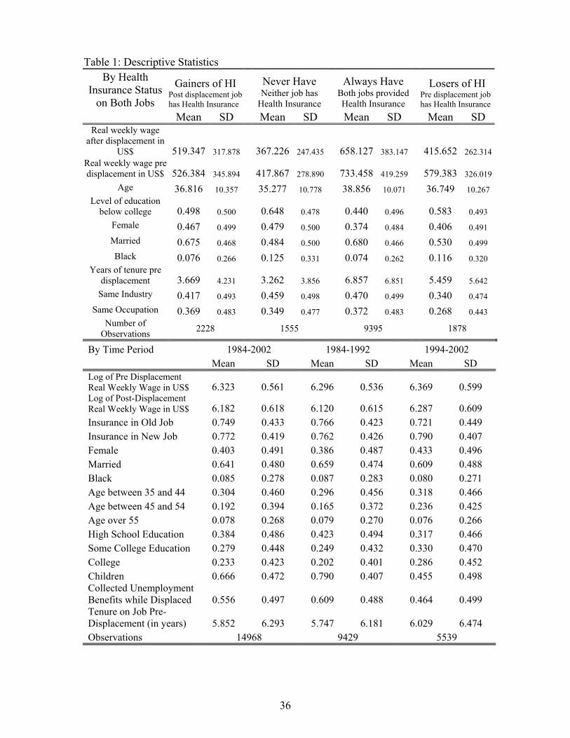
Table 1 presents summary statistics for portions of the sample used in this study. In

the top panel, the full sample is divided into four groups, based on their health insurance

provision pre and post displacement. The majority of the sample (64%) corresponds to

workers that received health insurance on both jobs and are called "Always". Workers

gaining health insurance following displacement constitute 14% of the sample, similarly

12% of the sample lost health insurance benefits with displacement and the remaining

10% did not receive health insurance at either job.

There are substantial differences between these groups in terms of their level of ed-

ucation, earnings, race and probability of switching industry and occupation following

displacement. The two groups of the sample that did not receive health insurance prior

to displacement have, on average, a lower level of education, a lower pre-displacement wage

and are more likely to be African American than groups which received health insurance

in both periods. Further, losing health insurance following displacement is associated with

both large wage losses and a higher likelihood of switching industry or occupation. Notice

13

that jobs pre and post displacement that offer health insurance provide higher wages.24

The usual explanation for this finding is that those employed in good jobs are likely to

differ from those in worse jobs on both observable and unobservable characteristics.25

In the second part of Table 1, we examine how the characteristics of the sample

differ between 1984-92 and 1994 onwards. Notice that, after 1994, the displaced workers

are more educated, slightly older and contain more females. Further, displaced workers

after 1994 are less likely to have children or receive unemployment benefits following

displacement. While age and education would suggest an increase in the propensity

to receive health benefits, not having children could serve to reduce the benefits from

receiving health coverage from an employer. Interestingly, more workers in our sample over

the last decade received health insurance following displacement, which is the opposite of

the pattern in the general labor market.

4 Results

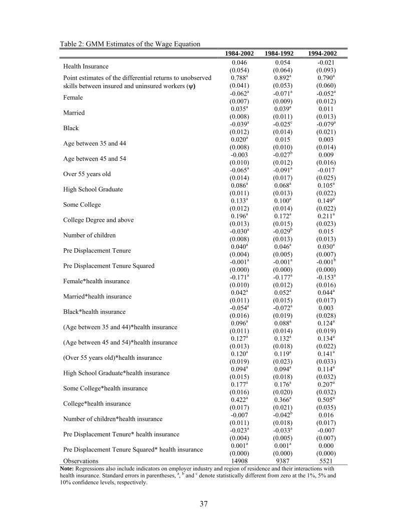
GMM estimates of equation (10) are displayed in Table 2. The full sample is presented

in column one, while columns two and three respectively present the subsamples for the

periods 1984-92 and 1994-2002. Health insurance is not significantly related to workers

wage in any of the samples. Only in the most recent decade is the sign of the coefficient

estimate consistent with the compensating wage differential theory. While this result

does not differ from most estimates found in the compensating differential literature, our

empirical strategy allows us to test some implicit assumptions within that literature.

The assumption that unobserved heterogeneity has a constant impact across sectors

underlies fixed effects, first difference and difference in difference propensity score match-

ing estimators. Our model treats the returns to this unobserved term in a more flexible

manner and parameter estimates of Ψ are presented in the second row of Table 2. For the

full pooled sample (presented in column one), Ψ is statistically different from one at the

1% confidence level, suggesting that we can directly reject the assumption that θNi = θHi ,

14

implying that unobserved skills are rewarded differently in the two sectors of the economy.

However, the constraint that Ψ is statistically different from one cannot be rejected at

the 1% confidence level for the 1984-1992 sample in the second column. The presence of

this omitted selection effect may be biasing the impacts reported in several longitudinal

studies. This suggests that, conditional on characteristics, some workers may have a com-

parative advantage in the health insurance sector, which, based on the differences in the

magnitude of the coefficient between columns two and three, appears to be of increasing

importance in recent years.

Further, consistent with earlier studies on the incidence of health insurance costs

on worker wages, there are substantial differences in how characteristics are rewarded

across the two sectors.26 There are lower returns to pre-displacement tenure and being

African American in firms that provide health insurance benefits. On the other hand,

being married, being older and being more educated yield higher returns in firms that

offer these benefits. While the positive return to marriage decreased slightly between

the sample periods, there was an approximate 27% increase in the returns to a college

education relative to 12 years of education or less in firms that provide benefits. In total,

the gap in the health insurance sector between college degree holders and individuals who

have fewer than 12 years of education rose over 30%, from 0.538 to 0.716. The wage gap

between males and females became smaller in both sectors following 1994. It is interesting

to note that while older workers received significant wage decreases in the sector that

does not provide health insurance prior to 1994, the relationship becomes statistically

insignificant for the period between 1994 and 2002. Finally, while the differential to being

African American increased after 1994, there is no additional wage offset in the health

insurance sector.

The estimates from Table 2 are used to decompose the unadjusted health insurance

wage gap into a true effect of health insurance on wages and a selection bias component

following equation (6). The first column of Table 3 presents the decomposition for the

15

entire sample period. Health insurance has substantial impacts on workers in the health

insurance sector that primarily operate through differential returns to observed charac-

teristics. For the full sample, over 80% of the effect of health insurance on workers in the

health insurance sector operates through this channel. Further, the role of unobserved

factors is limited.

The change in the components of the wage decomposition between 1984-1992 and 1994-

2002 in columns two and three of Table 3 presents several interesting findings. Between

these periods, the unadjusted wage gap has grown, which is, in part, (and consistent with

Farber and Levy (2000)) due to firms which stopped offering benefits over this time period

tended to be clustered in low-paying industries. The prime component that explains the

growth in the unadjusted wage gap between sectors is the substantial increase in the

returns to observed skills. The returns to these skills have more than doubled between

periods. Examining the second and third columns of Table 2, it is clear that these rewards

are being driven by the increased returns to a college education as well as returns to age,

which may proxy for total labor market experience.

Not only did the returns to observed skills rise across periods, but there was also a large

decrease in the amount of the gap that is attributable to selection bias. Overall selection

bias dropped by nearly 30%, from 0.179 to 0.127 driven by the differences in observed skills

across sectors. Information on the portion of selection bias attributable to observables and

unobservables is presented in rows six and seven of Table 3, respectively. Selection bias

due to unobservables measures the similarity in average unobserved attributes between

workers in the two sectors (i.e. θH and θN). The fifth row of Table 4 indicates that the gap

in these attributes has become smaller between the two sub-sample periods. On average,

workers employed in firms that offer health insurance have larger values associated with

unobserved attributes related to productivity¡θH¢than those employed in firms that do

not offer these benefits¡θN¢. Yet, the portion of selection bias due to unobserved skills

that cannot be accounted for by estimators such as OLS and matching rose by nearly 15%

16

between decades. Since θH > θN , and the health insurance wage gap is slightly higher for

individuals with higher unobserved skills, we would predict that the OLS estimates of the

compensating wage differential would be biased upwards.27

Our estimates are also used to decompose the unadjusted gap in variance of wages

between sectors. The results are presented in Table 4. The unadjusted gap appears small

and indicates that health insurance reduces the dispersion of wages between sectors.28

While the overall size of the difference between the variance of wages between sectors

becomes smaller after 1994, the role of the two major components of the decomposition,

the effect of health insurance on health insurance workers and selection bias, increases

markedly. In particular, the portion of selection bias due to differences in unobserved

skills and the direct effect of both observed and unobserved skills on the variance of

wages increase by over 50% between the periods. While workers appeared on average

to be increasingly more homogeneous across sectors in Table 3, the results in the fifth

row suggest that there is substantially more heterogeneity in the unobserved skills of

individuals working in the health insurance sector (relative to the other sector) after

1994.

In Table 3, we found that employers in the health insurance sector did not pay workers

differently on the basis of these unobserved skills and increasingly rewarded observed skills.

If employers assume that observed productivity skills are highly positively correlated with

unobserved skills it may be the case that this heterogeneity has led employers to increase

the reward to observed characteristics. While this should suggest that the variance in

the wages between the sectors would increase across the two sample periods, there is,

as reported in the second row of Table 4, a large offset since unobserved skills have

significantly reduced the variance of wages for health insurance workers in the health

insurance sector.

The findings in Table 4 are also consistent with selection operating on both sides

of the labor market, which rules out traditional selection correction or control function

17

estimators. The negative covariance in the sixth row indicates that observed and unob-

served skills are positively correlated in the sector that does not provide health insurance,

but negatively correlated in the health insurance sector. This is consistent with positive

selection among workers with low unobserved skills in the health insurance sector and

negative selection among workers with high observed skills. This selection becomes more

important over time as the size of the covariance terms increases by over 50% between

the sample periods. This positive selection may be a result of increased worker shopping

for positions that offer health insurance benefits and may have partially contributed to

the recent health insurance cost spiral for employers.

In our estimation, we used the average unionization rate in the industry the worker

was employed in pre-displacement to instrument for previous period wage. To assess

the suitability of our instrument we consider a simple OLS regression of the first stage

regression and run an F-test for the joint significance of the instrument. The results

are presented in Table 5 for the case with information on unionization coverage rates.

We ignore the specifications with interaction terms included in the instrument set since

overidentification tests occasionally reject the hypothesis that the instruments are valid.29

Coefficients on the instrument and exogenous regressors in both columns are reasonable

in sign and magnitude. The instruments are statistically significant predictors of pre-

displacement wages and the F-statistics on its significance is respectively above current

cutoffs (i.e. Staiger and Stock (1997)) for weak instruments for both the full sample and

pre-1994 sample.

Since the reliability of our estimates depends directly on the validity of our instrument,

the low F-statistic over post 1994 period is a concern, since it may indicate weak identifi-

cation. Weak identification could result in i) the GMM estimates being inconsistent and

biased towards the NLLS estimates,30 and ii) the test statistics for inference are inaccu-

rate. Regarding the first problem, not only is the coefficient on the instrument reported in

Table 5 significant at the 1% level but also a Hausman test rejects the consistency of the

18

NLLS estimates. Further, we attempted to correct the statistical inference problem using

Moreira (2003) conditional approach to construct tests of coefficients based on the con-

ditional distributions of nonpivotal statistics. If the instruments have low strength then

the confidence intervals should increase relative to those based on standard asymptotic

theory. We find that the length of the 95% confidence interval increased by only 16.8%,

a small margin which increases our confidence in the validity of the instrument. Taken

together, these diagnostics suggest that it is unlikely that the second period estimates are

due to a poor instrument.

An additional concern is that the average unionization rate in the industry the worker

was employed in pre-displacement may not be a suitable instrument, since it is related to

an individual’s own union status, which is implicitly contained in the residual. To examine

the robustness of our results, we replicated the full analysis accounting for individual union

status both pre and post displacement for the portion of the sample that provided this

information and our results did not change neither qualitatively, nor quantitatively.31

4.1 Worker Sorting and Health Insurance

4.1.1 Are Search Patterns in the DWS Consistent with Increased Worker

Sorting?

Testing directly for worker sorting is difficult without more detailed information on firms.

To present additional evidence that is consistent with the hypothesis of an increase in

worker sorting we contrast job search patterns between post displacement health insur-

ance receipt conditional on pre displacement health insurance receipt over time. We

hypothesize that if worker shopping has increased then individuals who gain health in-

surance following displacement should have longer searches. Due to the sampling criteria

change after 1994, it is hard to compare these past histories between the two sampling

periods and the results should be biased against our hypothesis, since longer job searches

are possible in the earlier data collections.

19

To draw comparisons we consider a difference in difference strategy. First, we con-

trast the length of job search between new health insurance recipients with individuals

who never receive health insurance. Second, we compare individuals who receive health

insurance pre and post displacement to individuals who lose health insurance after dis-

placement. The implicit assumption underlying this strategy is common trend, that is

that any changes in outcomes between these groups must be the result of health insurance

status post displacement. Essentially we estimate a regression model of the form

Yit = γ1 + x0itγ2 +HI 0itγ3 + (HIit ∗ t2)0γ4 + t2 + vit (12)

where Yit is weeks of job search and t2 is a dummy for the period after 1994. If γ4 > 0,

this would support the hypothesis that individuals who receive health insurance following

displacement post 1994 are associated with an increase in job search. We estimate equa-

tion (12) separately for individuals who had health insurance prior to displacement and

for those who did not have these benefits.

Column one of Table 6 presents differences in the experiences between jobs for in-

dividuals who lost health insurance following displacement versus those who had health

insurance in both jobs. Consistent with a story of increased job search, workers who found

employment in firms that offered health insurance search for approximately three more

weeks. Since the average job search in this period is 10.586 weeks, this is an increase of

approximately 30% from the mean. However, the results presented in column two that

compare new health insurance recipients to individuals who never received health insur-

ance, do not find any significant differences in length of job search after 1994 for new

recipients. As shown in Table 1, on average, the workers who gain health insurance post

displacement have the shortest searches. Not surprisingly, older workers search longer in

both subsamples as do workers with more tenure on the earlier job and less education, as

they may have been most scarred from the displacement.

20

4.1.2 Is the link between unobserved productivity attributes and health in-

surance coverage homogenous?

Understanding if individuals with lower unobserved productivity attributes are increas-

ingly sorting to jobs that provide health insurance benefits is clearly a question of policy

interest. While our data cannot directly address whether these individuals truly have lower

health status to determine if sorting may have contributed to the recent rise in health

insurance costs, we can examine whether the unobserved productivity characteristics of

workers are increasingly correlated with post-displacement jobs that provide benefits. We

consider estimation of

bθi = γ1 +HI 0itγ2 + (HIit ∗ t2)0γ3 + t02γ4 + vit (13)

where t2 is a dummy for the period after 1994 and bθi is the predicted individual timeinvariant characteristics obtained from OLS estimation of the following equation

θit = δ1 + θit−1δ2 + it (14)

where it is a random unobservable, θit is calculated using equation (9) and GMM es-

timates from the first column of Table 2.32 Table 7 present estimates of equation (13)

based on samples defined by pre-displacement health insurance status and age.

For the full sample in column one, we notice that, while health insurance is associated

with higher unobserved attributes (γ2 > 0), the recipients in the second time period

actually have lower values of θi (γ4 < 0). This indicates that individuals who have health

insurance in the second period have on average values of θi that are 0.043 lower then

the earlier time period. This effect is large and approximately equal to a 5% of the

standard deviation of θi. Columns four and seven present evidence that the magnitude

of this negative impact is not heterogeneous with respect to whether or not an individual

had health insurance pre-displacement. When we examine subsamples that are defined

by age several interesting patterns emerge. The estimates of γ3 in the third, sixth and

21

ninth columns demonstrate that there is a large decrease in θi associated with receiving

health insurance after 1994 for workers above 45. In contrast workers under the age of

45 either have γ3 estimates that are statistically insignificant (column eight) or of limited

economic significance (columns two and five). The results in Table 7 suggest that while on

average unobserved productivity attributes are greater in the period following 1994, there

is a significant negative association between these unobserved productivity attributes and

receiving employer provided health insurance after 1994. This effect is driven by workers

that are at least 45 years of age.33

Taken together, the results in this section suggest that, among individuals who have

health insurance in the period post 1994, they have i) lower values of θi, unobserved

productivity attributes that may include health status, and ii) the search for another

position that provides these benefits lasted an additional two weeks. We hypothesize that

these individuals are most likely familiar with health insurance benefits and increasingly

seek out jobs that offer this amenity. As we discuss in the concluding section, such non-

random sorting is likely the primary reason why we cannot find evidence of a compensating

differential in Table 4.

5 Conclusions

Surveys of workers consistently rank health insurance as far and away the most important

among all benefits offered in the workplace (Salisbury, 2001). Intuitively, health insurance

has the potential to influence numerous labor market decisions and many individuals may

be reluctant to consider working for companies that do not provide health benefits.34 At

the same time, employers are increasingly facing large increases in the costs of providing

these benefits. Hence, understanding how the provision of these benefits affects the labor

market has substantial policy and human resource implications.

In this paper, we extended the health economics literature on compensating differen-

tials by introducing an empirical approach that allows 1) both individual observed and

22

unobserved (to the econometrician) characteristics to be rewarded differently in different

sectors of the economy, and 2) selection to operate on both sides of the labor market. An

important feature of this model is that the estimates enable us to test several assump-

tions that are made with existing empirical strategies. We find that the assumption that

unobserved attributes are rewarded equally in both sectors which underlies fixed effects

and traditional differencing strategies is rejected. In addition, we find evidence that there

is substantial selection on unobserved characteristics, which rules out matching and OLS

strategies. Finally, we find that selection operates on both sides of the labor market, a

feature that cannot be accounted for by traditional control function estimators.

While we do not find any evidence of a health insurance compensating wage differential,

we observe that health insurance has increasingly influenced wage inequality. We present

evidence that the provision of health insurance is increasingly affecting the dispersion of

wages across sectors, which is consistent with the findings in the compensating differentials

literature that have explored the incidence question from the perspective of employers.

Estimates from our model are also used to decompose the wage gap between the sectors

and we find there are substantial changes in the selection of workers to firms that provide

health insurance benefits. Specifically, we observe that there has been increasing sorting

based on comparative advantage. Finally, we find that recently displaced workers are

searching nearly three weeks longer for jobs that provide health benefits and that these

workers on average have lower unobserved productivity attributes.

An important limitation of this study is that the impacts we estimate are applicable to

displaced workers only. The composition of displaced workers not only differs from other

workers in the labor market, but has also changed over time.35 Yet, it should be noted

that our finding of an increasing role of health insurance on wages is consistent with the

recent health economics literature that indicates that the recent rise in health insurance

premiums affects a variety of labor market outcomes.36 Consequently, it is likely our

findings have some limited external validity.

23

We do not view our failure to find evidence of a compensating differential despite

using a more general estimation approach as a rejection of the underlying theory. The

simple compensating differentials theory remains inconsistent with two empirical features

of the U.S. labor market. First, there is large variability in costs of health insurance

across similar firms. Understanding the sources of this variability may suggest additional

variables that may need to be accounted for in wage regressions. In this study, we find

strong evidence that the sorting of workers to jobs is consistent with comparative advan-

tage.37 While, sorting in the labor market is likely to lead to strong correlations between

observed and unobserved attributes of the individual with the corresponding variables of

their co-workers, our evidence also indicates that in recent years the distribution of these

unobserved attributes is more heterogeneous in the health insurance sector. Thus, sorting

to firms on the basis of preferences for health insurance is not perfect and there still may

remain heterogeneity at the firm level that is not a function of these individual specific

heterogeneities, suggesting that frictions exist in the labor market. Accounting for such

heterogeneity in addition to individual heterogeneity as well as the identification of the

impacts of endogenous group formation at firms has typically been ignored (in part due

to data limitations) in the health insurance compensating differentials literature.38

Second, employers cannot set employee specific compensation packages. An increasing

body of evidence suggests that there is likely substantial heterogeneity regarding prefer-

ences for health insurance benefits among workers within firms. For example, Gruber

and Lettau (2004) find that within firms, the median worker and workers in the highest

quantiles of salary exhibit a disproportionate amount of influence on decisions related to

health insurance coverage. These workers may also be willing to bear a disproportionate

amount of the costs through lower wages, and if these tastes can indeed be proxied by

observables such as salary, it may be useful to examine whether the tradeoff exists by

examining those most likely affected. For example, with longitudinal matched employee

and employer data it is possible to examine within firms how the estimated trade-off varies

24

across the salary distribution and how the distribution of residual wage dispersion varies

across firms that differ in both benefit provision and the cost of benefits.39 In conclusion,

future research needs to consider general empirical models with richer data sources to

determine whether the compensating differential truly exists as well as shed more light

on how health insurance provision affects the labor market.

25

Notes

1Between 2001 and 2004, premiums for family coverage shot up by 59 percent, com-

pared to a 9.7 percent gain in inflation and a 12.3 percent wage growth rate. See Kaiser

Family Foundation and Health Research and Educational Trust (2004) for details.2The Kaiser Family Foundation (2005) reports that only 60% of companies offered

health insurance to their employees in 2005, down from 69% in 2000. Gruber and McK-

night (2003) report that, in 1982, 44% of those who were covered by their employer-

provided health insurance had their costs fully financed by their employer, but by 1998

this had fallen to 28%. Cutler (2002) finds that the increasing employee costs for health

insurance resulted in employees declining coverage in the 1990s. Increased anecdotal

evidence suggests that this trade-off exists, and there are reports in the popular press

that firms have even made termination decisions based strictly on an individual’s health

behavior, such as smoking, in an effort to reduce health insurance costs (Armour (2005)).3Bundorf (2002) shows that higher wage workers are more likely to receive health in-

surance benefits. Gruber and Lettau (2004) find that the decision to offer health insurance

at the firm level depends on the prices faced by both the median worker and highly com-

pensated workers. Wiatrowski (1995) reports that medium and large establishments were

20% more likely to offer health insurance to full time employees relative to small establish-

ments. Dranove, Spier and Baker (2000) show that spousal coverage affects employment

decisions.4Currie and Madrian (1999) present a survey of the early cross sectional and longitu-

dinal compensating differential studies in the health economics literature. They conclude

that many of these studies did not have the appropriate data to estimate the magnitude

of the compensating differential.5Pauly (1986) suggests that the sorting of workers based on these tastes across sectors

is imperfect. Changes in the sorting process over time could partially explain the more

rapid increases in health insurance costs that may simultaneously affect the levels and

26

dispersion of salaries within firms that provide health insurance benefits. We discuss the

implications of imperfect sorting for the compensating differentials literature in the final

section.6The implications of absolute and comparative advantage as sorting mechanisms are

outlined in Willis (1986) and Sattinger (1993).7More generally, worker sorting could have profound impacts on the macroeconomy if

non market interactions exist, such as peer effects (e. g. Benabou (1996) and Kremer

(1993)).8See Jacobson, LaLonde and Sullivan (1993) for a careful analysis of earnings loss

following displacement and Farber (2003) for a survey of research on the experiences of

displaced workers.9Blue Cross and Blue Shield of Louisiana estimated that 200,000 residents who had

health insurance through the workplace lost their benefits due to Hurricane Katrina.10See Katz and Autor (1999) for an extensive overview of recent changes in the U.S.

wage structure.11An explicit characterization that would generate equations (1)-(4) in the context of

unions is provided in Robinson (1989). The model considered in this paper is based on

and discussed in further detail in Lemieux (1998). As noted by Lemieux (1998), the model

rules out individuals who change work voluntarily and focuses on involuntarily job loss.12Most econometric approaches assume constant slope coefficients which rules out com-

parative advantage.13Cutler (1995) reports that there exists huge variation in health insurance premiums

among otherwise identical firms that is partially the result of heterogeneity in the work-

force along health dimensions.14Let θi = θNi −ζ and θi =

θHi−ζϕwhere ζ is an orthogonal error component as in Lemieux

(1998).15Note that if one sets the Ψ = 1, this is equivalent to a first differenced estimation

27

procedure and imposes the assumption that unobserved attributes are rewarded in exactly

the same manner in both sectors. This assumption of constant rewards to unobserved

attributes also underlies fixed effects strategies. Note NLLS estimates of Ψ would be

biased even if the residuals are not serially correlated16Note as we discuss in the subsequent section our results do not change if we include

individual’s own union status pre and post displacement in the estimating equation. The

state level aggregates are also likely to be correlated with any firm level residual.17The estimates of βHI , βH , βN and ψ are obtained from equation (10) and summary sta-

tistics provide information on xH = E[xit|HIit = 1] and xN = E[xit|HIit = 0]. Similarly,

θH = E[θi|HIit = 1] and θN = E[θi|HIit = 0] where θi is calculated using the pre-

dicted regressors via equation (9). The gap in the variance of wages can also be de-

composed using the same information, and considering that ΣXH = V ar[xit|HIit =

1], ΣXN = V ar[xit|HIit = 0], σ2θH = V ar[θi|HIit = 1], σ2θN = V ar[θi|HIit = 0],

ΣXθH = Cov[xit, θi|HIit = 1], ΣXθN = Cov[xit, θi|HIit = 0], σ2H = V ar[ it|HIit = 1],

and σ2N = V ar[ it|HIit = 0].

18Hammermesh (1987) presents evidence from early DWS surveys that these displace-

ments indeed come as a surprise to the worker and firm.19The DWS does not contain hourly wage rates and we had to calculate this variable.

We assumed that health insurance is obtained from an individual’s primary position

and calculated the hourly wage rate for this position using information in the DWS.

Specifically, we took the difference between total wages and earnings from other jobs and

divided that by the average hours worked per week *weeks worked in a year.20Simon (2001) used data from 1984 to 2000 in her analysis. The CPS 2004 data

differ in their industry and occupation codes, which makes their addition to the analysis

impossible, since we use the average unionization rate in the industry as instrument.

Besides from the fact that we include an additional wave, the CPS 2002, our final sample

differs slightly from that in Simon (2001) as we apply a stricter definition of full time

28

work at the previous job. Note that the differences in the sample do not affect any of the

conclusions in Simon (2001).21In all waves of the survey, the health insurance information about the old job refers to

health insurance from the worker’s own employer. From 1984 to 1992, the new job health

insurance variable asked for whether any group health insurance was held, and from 1994

onwards asked whether any private health insurance was held at the present time.22Approximately 6% of matched individuals privately purchased insurance and nearly

31% received health insurance from a spouse. This subsample was removed from the

analysis. Note, our qualitative and quantitative results were robust if this subsample were

included in the estimation sample. This should reduce concerns regarding our implicit

assumption that for those individuals who could not be matched with the March CPS,

health insurance reported in the DWS was obtained from the primary employer.23Health care reform was a major component of Bill Clinton’s campaign in 1992. This

year also saw a marked slowdown in medical spending and the end to a period of rapid

growth in enrollment in managed care plan. While 5% of the privately insured were in

managed care in 1980 it had risen to approximately 75% in 1992 and that percentage has

been fairly stable since 1992.24More generally, there is substantial heterogeneity in unemployment spans and post

displacement job outcomes for displaced workers. Seitchik (1991) reports that while ap-

proximately 13of all displaced workers were reemployed within 5 weeks, about 1

3were not

reemployed until after more than 6 months. He also reports that 43% of workers displaced

between 1981 and 1986 had higher earnings on reemployed jobs in 1986 whereas over 30%

of workers were earning less than 34of their former wages.

25The difference in the tax treatment of wage and non-wage compensation also means

that highly compensated workers will equally be those who most value non-wage compen-

sation.26For example, Pauly and Herring (1999) report lower returns to experience in firms

29

that provide health insurance benefits, whereas Olson (2002) reports that being married

reduced wages for women working full time with health insurance.27In fact, the OLS estimate of the impact of health insurance in a simple wage equation

does exceed the true effect of health insurance on wages presented in Table 3. Note, the

OLS estimate may also suffer from bias if there are correlations between observed and

unobserved attributes.28Recall this is the gap in the variance of log hourly wages. This gap is small relative

to the gap in average log hourly wages.29As a robustness check we explored four alternative instrument sets. These sets were

chosen based on a suggestion in Lemieux (1998) to exploit the strict exogeneity condition

on the regressors of the model and use higher order terms and interaction terms of the

explanatory variables as instruments. While some of the instrument sets had slightly

better first stage properties the general pattern of our results (available from the authors)

were robust to the different instrument sets. Note, the selection of these instrument sets

relies on the plausibility of the strict exogeneity condition for identification.30The inconsistency of the GMM estimates depends on the relevance of the instrumental

variable. Hahn and Hausman (2003) show that the finite sample bias of these estimates

is inversely related to the first stage F-statistic.31Note that the inclusion of individual union status reduces efficiency as we use a smaller

sample and may also lead to additional concerns regarding endogeneity. Also note that

our underlying model has individuals choosing between sectors that differ only in their

health insurance provision and not union status.32Note that θis is measured with error since ξis is included on the right hand side

of equation (9). Since the model assumes that ηis in equation (3) is distributed iid

over time, this regression intuitively corresponds to regressing two variables with classical

measurement error on each other and obtaining the true signal by calculating the predicted

outcome (bθi).30

33We investigated the sensitivity of our results to the definition of t2.We found that for

workers above 45 the estimates of γ3 increase in absolute value as t2 indicates later time

periods (i.e. 1998 onwards).34Madrian (1994) finds that among married men with pregnant wives, those without

health insurance are twice as likely to switch jobs.35Farber (2001) describes how the characteristics of displaced workers have changed

over time.36For example, Cutler andMadrian (1998) and Baicker and Chandra (2006) find impacts

on hours worked and employment rates whereas Gruber and Krueger (1991) using similar

identification strategies with data from earlier time periods find no impacts.37There is, indeed, some evidence of worker sorting in the context of health insur-

ance within the health economics literature. Several studies (Marquis and Long (1995),

Monheit and Vistnes (1999) and Levy (1998)) show that workers with low preferences

for health insurance are disproportionately employed in firms that do not offer coverage.

Similarly evidence of employees sorting to firms based on health insurance benefits is

shown in Scott, Berger and Black (1989), Dranove, Spier and Baker (2000), and Levy

(1998). Yet, the evidence also indicates that sorting of workers to firms on the basis of

preferences for the compensation package is imperfect.38Since the individual unobserved attributes of wokers that sort into a firm are likely to

be similar, a negative within group correlation between observed and unobserved charac-

teristics of individuals will arise, even if these variables are uncorrelated in the population.

Using a general model to estimate hedonic equations, Epple (1987) demonstrates that

simply using group fixed effects is unlikely to be sufficient to overcome potential biases.39Alternatively one could examine the tradeoff over the age or tenure distribution within

firms. For example, one could hypothesize that consistent with the findings in Pauly and

Herring (1999), workers with high tenure may have lower labor market mobility and be

more willing to accept increased shares of health insurance costs over time.

31

References

[1] Armour, S., 2005. Trend, You smoke? You’re fired!. USA Today.http,//www.usatoday.com/money/companies/management/2005-05-11-smoke-usat_x.htm.

[2] Baicker, K. and Chandra A. 2006. The Labor Market Effects of Rising Health Insur-ance Premiums. Journal of Labor Economics 24, 609—634.

[3] Benabou, R., 1996. Heterogeneity, Stratification, and Growth, Macroeconomic Im-plications of Community Structure and School Finance. American Economic Review86, 584—609.

[4] Buchmueller, T. C., DiNardo, J., Valletta, R. G., 2002. Union Effects on Health In-surance Provision and Coverage in the United States. Industrial and Labor RelationsReview 55, 610—627.

[5] Bundorf, K. M., 2002. Employee Demand for Health Insurance and Employer HealthPlan Choices. Journal of Health Economics 21, 65—88.

[6] Currie, J., Madrian, B., 1999. "Health, Health Insurance and the Labor Market inD. Card and O. Ashenfelter (eds), Handbook of Labor Economics 3C, 3309-3407.

[7] Cutler, D. M., 2002. Employee Costs and the Decline in Health Care Coverage.NBER Working Paper No. 9036.

[8] Cutler, D. M. and Madrian, B. 1998. Labor Market Responses to Rising HealthInsurance Costs: Evidence on Hours Worked. RAND Journal of Economics 29, 509—30.

[9] Cutler, D. M., 1995. The Incidence of Adverse Medical Outcomes Under ProspectivePayment. Econometrica 63, 29—50.

[10] Dranove, D., Spier, K. E., Baker, L., 2000. Competition Among Employers OfferingHealth Insurance. Journal of Health Economics 19, 121—140.

[11] Employee Benefit Research Institute, 2002. Databook on Employee Benefits. 4th ed.http,//www.ebri.org/publications/books/index.cfm?fa=databook

[12] Epple, D. 1987. Hedonic Prices and Implicit Markets: Estimating Demand and Sup-ply Functions for Differentiated Products. Journal of Political Economy 95, 59-80.

[13] Farber, H. S., 2003. Job Loss in the United States, 1981-2001. NBER Working PaperNo. 9707.

32

[14] Farber, H. S., Levy, H., 2000. Recent Trends in Employer-Sponsored Health Insur-ance, Are Bad Jobs Getting Worse?. Journal of Health Economics 19, 93—119.

[15] Gruber, J., Lettau, M., 2004. How Elastic is the Firm’s Demand for Health Insurance.Journal of Public Economics 88, 1273—1293.

[16] Gruber, J., McKnight, R., 2003. Why Did Employee Health Insurance ContributionsRise?. Journal of Health Economics 22, 1085—1104.

[17] Gruber, J., 1994. The Incidence of MandatedMaternity Benefits.American EconomicReview 84, 622-641.

[18] Gruber, J., and Krueger, A. B., 1991. The incidence of mandated employer-providedinsurance: Lessons from workers’ compensation insurance. Tax Policy and the Econ-omy 5:111—43.

[19] Hahn, J., Hausman, J. 2003. Instrumental Variable Estimation with Valid and InvalidInstruments., MIT Department of Economics Working Paper No. 03-26.

[20] Hamermesh, D. S. 1987. The Costs of Worker Displacement. Quarterly Journal ofEconomics 102, 51-75.

[21] Jacobson, L., LaLonde, R., Sullivan, D., 1993. Earnings Losses of Displaced Workers.American Economic Review 83, 685—709.

[22] Kaiser Family Foundation and Health Research and Educational Trust, 2005. Em-ployer Health Benefits Survey. www.kff.org.

[23] Kaiser Family Foundation and Health Research and Educational Trust, 2004. Em-ployer Health Benefits Survey. www.kff.org.

[24] Katz L. F., Autor, D. H. 1999. Changes in the Wage Structure and Earnings In-equality, in O. Ashenfelter and D. Card, eds., Handbook of Labor Economics 3A,1463-1555.

[25] Kremer, M., 1993. The O-Ring Theory of Economic Development. Quarterly Journalof Economics 108, 551—576.

[26] Lemieux, T., 1998. Estimating the Effects of Unions on Wage Inequality in a PanelData Model with Comparative Advantage and Nonrandom Selection. Journal of La-bor Economics 16, 261—291.

[27] Levy, H., 1998. Who Pays for Health Insurance? Employee Contributions to HealthInsurance Premiums. Princeton University Industrial Relations Section Working Pa-per 398.

33

[28] Madrian, B. C., 1994. Employment-Based Health Insurance and Job Mobility: IsThere Evidence of Job-Lock? Quarterly Journal of Economics 109, 27-54.

[29] Marquis, M. S., Long, S. H., 1995. Worker Demand for Health Insurance in theNon-Group Market. Journal of Health Economics 14, 47—63.

[30] Monheit, A. C., Vistnes, J.C., 1999. Health Insurance Availability at the Workplace,How Important are Workers Preferences. Journal of Human Resources 34, 770—785.

[31] Moreira, Marcelo. 2003. A conditional likelihood ratio test for structural models.Econometrica 71, no. 4:1027—48.

[32] Olson, C. A., 2002. DoWorkers Accept LowerWages in Exchange for Health Benefits.Journal of Labor Economics 20, S91—S114.

[33] Oyer, P., 2004. Recall Bias Among Displaced Workers. Economics Letters 82, 392—397.

[34] Pauly, M. V., 2001. Making Sense of a Complex System, Empirical Studies ofEmployment-Based Health Insurance. International Journal of Health Care Financeand Economics 1, 333—339.

[35] Pauly, M., Herring, B., 1999. Pooling Health Insurance Risks. American EnterpriseInstitute Press, Washington, DC.

[36] Pauly, M. V. 1986. Taxation, Health Insurance, and Market Failure in the MedicalEconomy. Journal of Economic Literature 24, 629-675.

[37] Robinson, C., 1989. The Joint Determination of Union Status and Union Wage Ef-fects, Some Tests of Alternative Models. Journal of Political Economy 97, 639—67.

[38] Salisbury, D. L. 2001. EBRI Research Highlights: Retirement and Health Data Em-ployee Benefit Research Institute (EBRI) EBRI Special Report SR-36, and EBRIIssue Brief No. 229.

[39] Sattinger, M, 1993. Assignment Models of the Distribution of Earnings. Journal ofEconomic Literature 31 831-880.

[40] Scott, F., Berger, M. C., Black, D., 1989. Effects of the Tax Treatment of FringeBenefits on Labor Market Segmentation. Industrial and Labor Relations Review 42,216—229.

[41] Seitchik, A. 1991. Who Are Displaced Workers? in J. T. Addison, ed., Job 51 Dis-placement: Consequences and Implications for Policy. Detroit: Wayne State Univer-sity Press.

34

[42] Sheiner L. (1999), “Health Care Costs, Wages and Aging,” Federal Reserve Board ofGovernors #99-19, Washington D. C.

[43] Simon, K., 2001. Involuntary Job Change and Employer Provided Health Insurance;Evidence of a Wage/Fringe Benefit Tradeoff?. International Journal of Health CareFinance and Economics 1, 249—271.

[44] Staiger, D., Stock, J.H., 1997. Instrumental Variables Regression with Weak Instru-ments. Econometrica 65, 557—586.

[45] Wiatrowski, W. J., 1995. Who Really Has Access to Employer-Provided Health Ben-efits?. Monthly Labor Review 118, 36—44.

[46] Willis, R. J. 1986. Wage Determinants: A Survey and Reinterpretation of HumanCapital Earnings Functions. in O Ashenfelter and R Layard (eds), Handbook of LaborEconomics 1, 525-602.

35

36

Table 1: Descriptive Statistics By Health

Insurance Status on Both Jobs

Gainers of HI Post displacement job has Health Insurance

Never Have Neither job has

Health Insurance

Always Have Both jobs provided Health Insurance

Losers of HI Pre displacement job has Health Insurance

Mean SD Mean SD Mean SD Mean SD Real weekly wage

after displacement in US$ 519.347 317.878 367.226 247.435 658.127 383.147

415.652 262.314

Real weekly wage pre displacement in US$ 526.384 345.894 417.867 278.890 733.458 419.259 579.383 326.019

Age 36.816 10.357 35.277 10.778 38.856 10.071 36.749 10.267 Level of education

below college 0.498 0.500 0.648 0.478 0.440 0.496 0.583 0.493 Female 0.467 0.499 0.479 0.500 0.374 0.484 0.406 0.491 Married 0.675 0.468 0.484 0.500 0.680 0.466 0.530 0.499 Black 0.076 0.266 0.125 0.331 0.074 0.262 0.116 0.320

Years of tenure pre displacement 3.669 4.231 3.262 3.856 6.857 6.851 5.459 5.642

Same Industry 0.417 0.493 0.459 0.498 0.470 0.499 0.340 0.474 Same Occupation 0.369 0.483 0.349 0.477 0.372 0.483 0.268 0.443

Number of Observations 2228 1555 9395 1878

By Time Period 1984-2002 1984-1992 1994-2002 Mean SD Mean SD Mean SD Log of Pre Displacement Real Weekly Wage in US$ 6.323 0.561 6.296 0.536 6.369 0.599 Log of Post-Displacement Real Weekly Wage in US$ 6.182 0.618 6.120 0.615 6.287 0.609 Insurance in Old Job 0.749 0.433 0.766 0.423 0.721 0.449 Insurance in New Job 0.772 0.419 0.762 0.426 0.790 0.407 Female 0.403 0.491 0.386 0.487 0.433 0.496 Married 0.641 0.480 0.659 0.474 0.609 0.488 Black 0.085 0.278 0.087 0.283 0.080 0.271 Age between 35 and 44 0.304 0.460 0.296 0.456 0.318 0.466 Age between 45 and 54 0.192 0.394 0.165 0.372 0.236 0.425 Age over 55 0.078 0.268 0.079 0.270 0.076 0.266 High School Education 0.384 0.486 0.423 0.494 0.317 0.466 Some College Education 0.279 0.448 0.249 0.432 0.330 0.470 College 0.233 0.423 0.202 0.401 0.286 0.452 Children 0.666 0.472 0.790 0.407 0.455 0.498 Collected Unemployment Benefits while Displaced 0.556 0.497 0.609 0.488 0.464 0.499 Tenure on Job Pre-Displacement (in years) 5.852 6.293 5.747 6.181 6.029 6.474 Observations 14968 9429 5539

37

Table 2: GMM Estimates of the Wage Equation 1984-2002 1984-1992 1994-2002

Health Insurance 0.046 (0.054)

0.054 (0.064)

-0.021 (0.093)

Point estimates of the differential returns to unobserved skills between insured and uninsured workers (ψ)

0.788a (0.041)

0.892a (0.053)

0.790a (0.060)

Female -0.062a (0.007)

-0.071a (0.009)

-0.052a (0.012)

Married 0.035a (0.008)

0.039a (0.011)

0.011 (0.013)

Black -0.039a (0.012)

-0.025c (0.014)

-0.079a (0.021)

Age between 35 and 44 0.020a (0.008)

0.015 (0.010)

0.003 (0.014)

Age between 45 and 54 -0.003 (0.010)

-0.027b (0.012)

0.009 (0.016)

Over 55 years old -0.065a (0.014)

-0.091a (0.017)

-0.017 (0.025)

High School Graduate 0.086a (0.011)

0.068a (0.013)

0.105a (0.022)

Some College 0.133a (0.012)

0.100a (0.014)

0.149a (0.022)

College Degree and above 0.196a (0.013)

0.172a (0.015)

0.211a (0.023)

Number of children -0.030a (0.008)

-0.029b (0.013)

0.015 (0.013)

Pre Displacement Tenure 0.040a (0.004)

0.046a (0.005)

0.030a (0.007)

Pre Displacement Tenure Squared -0.001a (0.000)

-0.001a (0.000)

-0.001b (0.000)

Female*health insurance -0.171a (0.010)

-0.177a (0.012)

-0.153a (0.016)

Married*health insurance 0.042a (0.011)

0.052a (0.015)

0.044a (0.017)

Black*health insurance -0.054a (0.016)

-0.072a (0.019)

0.003 (0.028)

(Age between 35 and 44)*health insurance 0.096a (0.011)

0.088a (0.014)

0.124a (0.019)

(Age between 45 and 54)*health insurance 0.127a (0.013)

0.132a (0.018)

0.134a (0.022)

(Over 55 years old)*health insurance 0.120a (0.019)

0.119a (0.023)

0.141a (0.033)

High School Graduate*health insurance 0.094a (0.015)

0.094a (0.018)

0.114a (0.032)

Some College*health insurance 0.177a (0.016)

0.176a (0.020)

0.207a (0.032)

College*health insurance 0.422a (0.017)

0.366a (0.021)

0.505a (0.035)

Number of children*health insurance -0.007 (0.011)

-0.042b (0.018)

0.016 (0.017)

Pre Displacement Tenure* health insurance -0.023a (0.004)

-0.033a (0.005)

-0.007 (0.007)

Pre Displacement Tenure Squared* health insurance 0.001a (0.000)

0.001a (0.000)

0.000 (0.000)

Observations 14908 9387 5521 Note: Regressions also include indicators on employer industry and region of residence and their interactions with health insurance. Standard errors in parentheses, a, b and c denote statistically different from zero at the 1%, 5% and 10% confidence levels, respectively.

38

Table 3: Decomposition of the Unadjusted Weekly Wage Gap 1984-2002 1984-1992 1994-2002 Effect of health insurance on workers in health insurance sector:

1. Compensating Wage Differential, HIβ 0.046 0.054 -0.021

2. Effect of observed skills, ( )NHHx ββ −' 0.203 0.156 0.318

3. Effect of unobserved skills, ( ) Hθψ 1− 0.008 0.000 0.015 Total effect 0.257 0.210 0.312 Selection bias: 4. Differences in observed skills, ( ) N

NH xx β'' − 0.112 0.132 0.089

5. Differences in unobserved skills, ( )NH θθ − 0.035 0.047 0.038 Total bias 0.147 0.179 0.127 Unadjusted wage gap (WG) 0.404 0.389 0.439 Note: The decomposition is based on equation (6) and we use the estimates presented in Table 2 to construct each component.

39

Table 4: Decomposition of the Unadjusted Variance of Weekly Wages Gap 1984-2002 1984-1992 1994-2002 Effect of health insurance on workers in health insurance sector:

1. Effect of observed skills, N

XNNH

XHH ββββ Σ−Σ ''

0.058 0.043 0.074

2. Effect of unobserved skills, ( ) 22 1Hθ

σ−ψ -0.119 -0.047 -0.129

3. Covariance term, ( ) HXNH

θβψβ Σ− '2 0.004 0.005 0.006 Total effect -0.056 0.002 -0.049 Selection bias: 4. Differences in observed skills,

( ) NXNXH

N ββ Σ−Σ' 0.001 0.002 0.000

5. Differences in unobserved skills, 22NH θθ σσ − 0.065 0.000 0.064

6. Covariance term, ( )NXHXN

θθβ Σ−Σ'2 -0.022 -0.015 -0.024 Total bias 0.044 -0.014 0.039 Difference in residual variance, 22

NH σσ − -0.001 -0.002 0.000 Unadjusted variance gap (WG) -0.013 -0.014 -0.009 Note: The decomposition is based on equation (7) and we use the estimates presented in Table 2 to construct each component.

40

Table 5: First Stage Regressions of Pre Displacement Wage Assuming 1=ψ

Time Period 1984-2002 1984-1992 1994-2002 Unionization Rate in Pre-Displacement Industry

1.27*10E-3a (3.0*10E-4)

2.32*10E-3a (3.5*10E-4)

-1.62*10E-3a (6.6*10E-4)

Health Insurance Pre Displacement 0.236a (0.035)

0.230a (0.044)

0.160a (0.062)

Married 0.061a (0.022)

0.088a (0.028)

0.054 (0.037)

Black -0.037 (0.027)

-0.087a (0.033)

0.069 (0.049)

Age between 35 and 44 0.067a (0.022)

0.072a (0.028)

0.066c (0.039)

Age between 45 and 54 0.105a (0.031)

0.113a (0.038)

0.122b (0.053)

Over 55 years old 0.045 (0.045)

0.028 (0.053)

0.080 (0.079)

High School Graduate 0.134a (0.023)

0.118a (0.029)

0.154a (0.043)

Some College 0.252a (0.027)

0.241a (0.035)

0.281a (0.041)

College Degree and above 0.447a (0.035)

0.387a (0.045)

0.537a (0.056)

Pre Displacement Tenure 0.028a (0.005)

0.030a (0.006)

0.022b (0.009)

Pre Displacement Tenure Squared -7.4*10E-4a (2.0*10E-4)

-8.8*10E-4a (2.2*10E-4)

-4.2*10E-4 (4.3*10E-4)

Married* health insurance 0.030 (0.021)

0.017 (0.029)

0.024 (0.035)

Black* health insurance -0.011 (0.029)

-0.018 (0.035)

0.042 (0.052)

(Age between 35 and 44)* health insurance 0.018 (0.022)

-0.006 (0.027)

0.062c (0.038)

(Age between 45 and 54)* health insurance 0.018 (0.028)

-0.041 (0.036)

0.102b (0.044)

(Over 55 years old)* health insurance -0.019 (0.040)

-0.037 (0.049)

0.053 (0.068)

High School Graduate* health insurance 0.003 (0.026)

0.003 (0.031)

0.045 (0.051)

Some College* health insurance -0.026 (0.029)

-0.043 (0.037)

0.020 (0.051)

College degree* health insurance 0.048 (0.033)

0.051 (0.042)

0.095c (0.058)

Pre Displacement Tenure* health insurance -0.006 (0.005)

-0.011c (0.006)

2.1*10E-3 (0.010)

Pre Displacement Tenure Squared* health insurance

2.6*10E-4 (2.1*10E-4)

4.6*10E-4b (2.3*10E-4)

-1.32*10E-4 (4.5*10E-4)

Constant 5.678a (0.045)

5.816a (0.060)

5.755a (0.072)

Observations R-Squared First Stage F- statistic on the Instrument

14908 0.378 16.06

9387 0.374 39.84

5521 0.400 6.09

Note: Regressions include information on gender, Hispanic, family composition, employer industry, unemployment insurance use, region of residence indicators and their interactions with health insurance. Robust standard errors in parentheses and . a, b and c denote statistically different from zero at the 1%, 5% and 10% confidence levels, respectively.

41

Table 6: Linear Difference in Difference Estimates of the Impact of Health Insurance Receipt Post 1994 on Job Search Activity Following Displacement

Sample

Health Insurance Pre Displacement

No Health Insurance Pre Displacement

Health Insurance (γ2) -5.480a (0.803)

0.393 (0.925)

Post 1994 (γ3) -9.346a (1.216)

-5.284a (1.045)

Health Insurance * Post 1994 (γ4) 2.761b (1.282)

-1.981 (1.347)

Married -0.112 (0.450)

1.362b (0.689)

Black -0.071 (0.565)

0.024 (0.820)

Age between 35 and 44 4.589a (0.907)

4.291a (1.466)

Age between 45 and 54 1.050b (0.515)

1.490c (0.827)

Over 55 years old 2.520a (0.644)

2.037b (1.000)

High School Graduate 4.734a (0.963)

2.219 (1.494)

Some College -6.068a (0.958)

-2.019c (1.150)

College Degree and Above -7.233a (0.957)

-2.189c (1.256)

Pre Displacement Tenure 0.480a (0.095)

0.735a (0.206)

Pre Displacement Tenure Squared -0.012a (0.003)

-0.025a (0.008)

Constant 23.112a (1.242)

11.683a (1.408)

Observations Adjusted R-Squared

10037 0.065

3242 0.045

Note: Regressions include information on gender, Hispanic, family composition, employer industry, unemployment insurance use and region of residence indicators. Robust standard errors in parentheses, a, b and c denote statistically different from zero at the 1%, 5% and 10% confidence levels, respectively.

42

Table 7: Nonparametric difference in difference estimates of the impact of health insurance receipt after 1994 on individual specific time invariant unobserved productivity attributes θi Sample

Full Sample Health Insurance Pre Displacement

No Health Insurance Pre Displacement

All Ages Aged 20-44

Aged 45-64

All Ages Aged 20-44

Aged 45-64

All Ages Aged 20-44

Aged 45-64

Health Insurance post displacement (γ2)

0.031a (0.568)

0.030a (0.625)

0.038a (1.323)

0.029a (0.732)

0.029a (0.816)

0.034b (1.630)

-0.010 (0.976)

-0.013 (1.060)

0.001 (2.414)

Health Insurance post displacement after 1994 (γ3)

-0.042a (0.887)

-0.023a (0.995)

-0.100a (1.921)

-0.045a (1.190)

-0.035b (1.352)

-0.077a (2.479)

-0.044a (1.433)

-0.012 (1.579)

-0.138a (3.274)

Indicator variable for Period Following 1994 (γ4)

0.063a (0.763)

0.043a (0.846)

0.127a (1.704)

0.071a (1.074)

0.057a (1.214)

0.115a (2.273)

0.061a (1.079)

0.036a (1.165)

0.147a (2.608)

Number of Observations 14968 10930 4038 11216 8064 3152 3752 2866 886 Adjusted R-squared 0.0063 0.0053 0.0140 0.0064 0.0053 0.0118 0.0117 0.0062 0.0454 Note: Robust standard errors *10E-3 are in parentheses. a, b and c denote statistically different from zero at the 1%, 5% and 10% confidence levels, respectively.