This article appeared in a journal published by Elsevier. The attachedcopy is furnished to the author for internal non-commercial researchand education use, including for instruction at the authors institution

and sharing with colleagues.

Other uses, including reproduction and distribution, or selling orlicensing copies, or posting to personal, institutional or third party

websites are prohibited.

In most cases authors are permitted to post their version of thearticle (e.g. in Word or Tex form) to their personal website orinstitutional repository. Authors requiring further information

regarding Elsevier’s archiving and manuscript policies areencouraged to visit:

http://www.elsevier.com/copyright

Author's personal copy

Electric Power Systems Research 79 (2009) 531–538

Contents lists available at ScienceDirect

Electric Power Systems Research

journa l homepage: www.e lsev ier .com/ locate /epsr

Wind energy conversion system regulation via LMI fuzzy pole cluster approach

Ahmad Hussien Besheera,∗, Hassan M. Emarab, Mamdouh Mohamed Abdel Azizb

a Environmental Studies and Research Institute, Mounoufia University, Sadat City, Sixth Zone, Egyptb Faculty of Engineering, Cairo University, 12613 P.O. Box, Giza, Egypt

a r t i c l e i n f o

Article history:Received 2 February 2006Received in revised form 20 April 2008Accepted 7 August 2008Available online 18 October 2008

Keywords:Fuzzy systemPole clusterWECST–S modelState feedback

a b s t r a c t

This paper addresses the design of fuzzy state feedback controller that has not only the ability to stabilizethe fuzzy model/system but also to control the transient behavior and closed loop poles location for windenergy conversion system (WECS) that presents interesting control demands and exhibits intrinsic non-linear characteristics. The proposed fuzzy controller is employed to regulate indirectly the power flowin the grid connected WECS by regulating the DC current flows in the interconnected DC link. First, aTakagi–Sugeno fuzzy model is employed to represent the non-linear WECS. Then a model-based fuzzycontroller design utilizing the concept of parallel-distributed compensation is developed. Satisfactorytime response and closed loop damping over wide operating range are achieved by forcing the closedloop poles into a suitable sub-region of the complex frequency plane. Sufficient stability conditions areexpressed in terms of linear matrix inequalities (LMI’s) which can be solved very efficiently using convexoptimization techniques. The design procedures are applied to a dynamic model of a typical wind energyconversion system to illustrate the feasibility and the effectiveness of the proposed control techniques viasimulation example.

© 2008 Elsevier B.V. All rights reserved.

1. Introduction

In the world of today there is a need for alternatives to the largecoal and oil fired power plants. Renewable energy is one way togo, and in particular wind turbines have proven to be a solution[1]. The arrival of the new power devices technologies, new circuittopologies and novel control strategies are contributing to the suc-cess of the wind generation technology. The control of wind energyconversion system is considered an interesting application area forcontrol theory and engineering because the wind energy conver-sion system consists of many dynamics integrated or combinedtogether (such as structural dynamics, drive train dynamics, gener-ator dynamics and the dynamics of the control system hardware).These dynamics are lightly damped, they are mainly dependenton wind speed. These dynamics have also high non-linear nature.The objectives for the control system are unusual in that it is notthe dynamics induced by transient loads that are required to beminimized but the fatigue damage induced by them. Finally, con-trol must be achieved at minimum expense and hence both controlmeasurement and control actuator hardware are severely restricted[2].

∗ Corresponding author.E-mail addresses: ahtawfeek@yahoo.com (A.H. Besheer),

hmrashad@ieee.org (H.M. Emara).

The control objectives of WECS can be classified according to thefollowing criteria:

(1) Fixed speed operation or variable speed operation of the windturbine.

(2) Operation of wind turbine is below or above rated wind speed.(3) Type of WECS topology (stand alone, hybrid or grid connected).

Fixed speed wind energy conversion system (FSWECS) is widelyused for power rating up to 2 MW. This concept is relatively simple,robust and cheap. It has the advantage of low maintenance cost.However, there are some drawbacks; the wind turbine has to oper-ate at constant speed; it requires a stiff power grid to enable stableoperation and implies more expensive mechanical construction inorder to be capable to absorb high mechanical stress. Furthermore,with constant speed there is only one wind velocity that results inan optimum tip speed ratio. Therefore, the wind turbine is oftenoperated off its optimum performance [3].

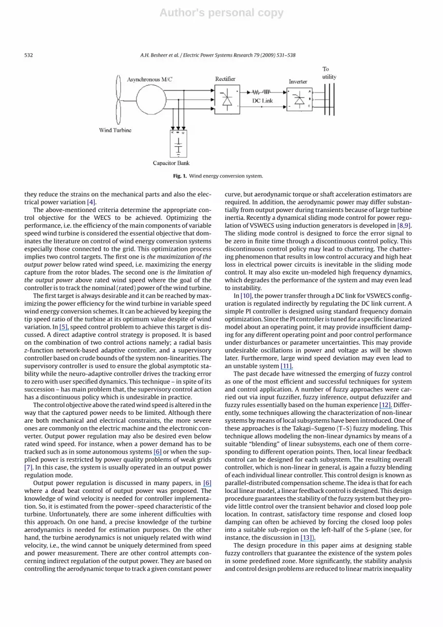
Variable speed wind energy conversion system (VSWECS) isbasically composed of wind turbine coupled to electric generator.The electrical generator output can be connected to the grid bymeans of modern converter system. This configuration is shown inFig. 1. Systems with synchronous or asynchronous generator, a rec-tifier, a DC interconnected circuit and a grid commutated inverterallow the turbine rotating speed to be decoupled from the gridfrequency. These are becoming more and more important because

0378-7796/$ – see front matter © 2008 Elsevier B.V. All rights reserved.doi:10.1016/j.epsr.2008.08.008

Author's personal copy

532 A.H. Besheer et al. / Electric Power Systems Research 79 (2009) 531–538

Fig. 1. Wind energy conversion system.

they reduce the strains on the mechanical parts and also the elec-trical power variation [4].

The above-mentioned criteria determine the appropriate con-trol objective for the WECS to be achieved. Optimizing theperformance, i.e. the efficiency of the main components of variablespeed wind turbine is considered the essential objective that dom-inates the literature on control of wind energy conversion systemsespecially those connected to the grid. This optimization processimplies two control targets. The first one is the maximization of theoutput power below rated wind speed, i.e. maximizing the energycapture from the rotor blades. The second one is the limitation ofthe output power above rated wind speed where the goal of thecontroller is to track the nominal (rated) power of the wind turbine.

The first target is always desirable and it can be reached by max-imizing the power efficiency for the wind turbine in variable speedwind energy conversion schemes. It can be achieved by keeping thetip speed ratio of the turbine at its optimum value despite of windvariation. In [5], speed control problem to achieve this target is dis-cussed. A direct adaptive control strategy is proposed. It is basedon the combination of two control actions namely; a radial basisz-function network-based adaptive controller, and a supervisorycontroller based on crude bounds of the system non-linearities. Thesupervisory controller is used to ensure the global asymptotic sta-bility while the neuro-adaptive controller drives the tracking errorto zero with user specified dynamics. This technique – in spite of itssuccession – has main problem that, the supervisory control actionhas a discontinuous policy which is undesirable in practice.

The control objective above the rated wind speed is altered in theway that the captured power needs to be limited. Although thereare both mechanical and electrical constraints, the more severeones are commonly on the electric machine and the electronic con-verter. Output power regulation may also be desired even belowrated wind speed. For instance, when a power demand has to betracked such as in some autonomous systems [6] or when the sup-plied power is restricted by power quality problems of weak grids[7]. In this case, the system is usually operated in an output powerregulation mode.

Output power regulation is discussed in many papers, in [6]where a dead beat control of output power was proposed. Theknowledge of wind velocity is needed for controller implementa-tion. So, it is estimated from the power–speed characteristic of theturbine. Unfortunately, there are some inherent difficulties withthis approach. On one hand, a precise knowledge of the turbineaerodynamics is needed for estimation purposes. On the otherhand, the turbine aerodynamics is not uniquely related with windvelocity, i.e., the wind cannot be uniquely determined from speedand power measurement. There are other control attempts con-cerning indirect regulation of the output power. They are based oncontrolling the aerodynamic torque to track a given constant power

curve, but aerodynamic torque or shaft acceleration estimators arerequired. In addition, the aerodynamic power may differ substan-tially from output power during transients because of large turbineinertia. Recently a dynamical sliding mode control for power regu-lation of VSWECS using induction generators is developed in [8,9].The sliding mode control is designed to force the error signal tobe zero in finite time through a discontinuous control policy. Thisdiscontinuous control policy may lead to chattering. The chatter-ing phenomenon that results in low control accuracy and high heatloss in electrical power circuits is inevitable in the sliding modecontrol. It may also excite un-modeled high frequency dynamics,which degrades the performance of the system and may even leadto instability.

In [10], the power transfer through a DC link for VSWECS config-uration is regulated indirectly by regulating the DC link current. Asimple PI controller is designed using standard frequency domainoptimization. Since the PI controller is tuned for a specific linearizedmodel about an operating point, it may provide insufficient damp-ing for any different operating point and poor control performanceunder disturbances or parameter uncertainties. This may provideundesirable oscillations in power and voltage as will be shownlater. Furthermore, large wind speed deviation may even lead toan unstable system [11].

The past decade have witnessed the emerging of fuzzy controlas one of the most efficient and successful techniques for systemand control application. A number of fuzzy approaches were car-ried out via input fuzzifier, fuzzy inference, output defuzzifer andfuzzy rules essentially based on the human experience [12]. Differ-ently, some techniques allowing the characterization of non-linearsystems by means of local subsystems have been introduced. One ofthese approaches is the Takagi–Sugeno (T–S) fuzzy modeling. Thistechnique allows modeling the non-linear dynamics by means of asuitable “blending” of linear subsystems, each one of them corre-sponding to different operation points. Then, local linear feedbackcontrol can be designed for each subsystem. The resulting overallcontroller, which is non-linear in general, is again a fuzzy blendingof each individual linear controller. This control design is known asparallel-distributed compensation scheme. The idea is that for eachlocal linear model, a linear feedback control is designed. This designprocedure guarantees the stability of the fuzzy system but they pro-vide little control over the transient behavior and closed loop polelocation. In contrast, satisfactory time response and closed loopdamping can often be achieved by forcing the closed loop polesinto a suitable sub-region on the left-half of the S-plane (see, forinstance, the discussion in [13]).

The design procedure in this paper aims at designing stablefuzzy controllers that guarantee the existence of the system polesin some predefined zone. More significantly, the stability analysisand control design problems are reduced to linear matrix inequality

Author's personal copy

A.H. Besheer et al. / Electric Power Systems Research 79 (2009) 531–538 533

(LMI) problems [14]. Numerically, the LMI problems can be solvedvery efficiently by means of powerful tools available to date inthe mathematical programming literature. Since LMI’s intrinsicallyreflect constraints rather than optimality it offers more flexibil-ity for combining several constraints on the closed loop system.Therefore, by solving the stability LMI’s and pole cluster con-straint LMI’s simultaneously, the feedback gains which guaranteeglobal asymptotic stability and satisfy the desired performance aredetermined.

2. Dynamic modeling of WECS

This section presents briefly the dynamic modeling of each sub-system for the proposed WECS. The WECS adopted in this work isshown in Fig. 1. It consists of three blades horizontal axis wind tur-bine that drives a self-excited induction generator connected to thegrid via AC–DC–AC link scheme.

The torque at the turbine shaft neglecting losses in the drivetrain is given by [15]:

Tm = 0.5��CtR3V2

w (1)

where Tm is the turbine mechanical torque, � is the air density, R isthe turbine radius, Ct is the turbine torque coefficient and Vw is thewind velocity.

The non-linear dynamical model of the induction machine inthe d–q reference frame for the proposed WECS when generatingcan be stated as follows:

piqs = −k1rsiqs − (ωe + k2Lmωr)ids + k2rriqr − k1Lmωridr (2)

pids = (ωe + k2Lmωr)iqs − k1rsids + k1Lmωriqr + k2rridr − k1vds (3)

piqr = k2rsiqs+Lsk2ωrids −[

rr + Lmk2rr

Lr

]iqr+(Lsk1ωr − ωe)idr (4)

piqr = −Lsk2ωriqs + k2rsids − (Lsk1ωr − ωe)iqr

− rr + Lmk2rr

Lridr + k2vds (5)

pωr = −B

jωr + 3N2Lm

8j(iqsidr − idsiqr) + N

2jTm (6)

where k1 = Lr/(LsLr − L2m) and k2 = Lm/(LsLr − L2

m).The above equations are derived assuming that the initial ori-

entation of the q–d synchronously rotating reference frame issuch that the d-axis is aligned with stator terminal voltage pha-sor (i.e. vqs = 0). The AC–DC–AC link scheme used in this paperconsists of a controlled rectifier, a DC link reactor and a con-trolled line commutated inverter. The dynamical equations ofself-excitation capacitance and the DC link can be described asfollows:

pvds = idc

C(7)

LDCpiDC + RDCiDC = vR − vI (8)

The detailed of these above equation and its parameters canbe found in [10] and [16]. The entire symbols for WECS usedin this paper are given in Appendix. Based on Eqs. (2)–(8),the order of the non-linear model that describes the proposedWECS is 7th order. The Local linear models of the WECS can bederived by applying Taylor linearization technique. A fuzzy con-troller based on these local models is derived in the followingsection.

3. Proposed control strategy

For non-linear systems, a good approximation is provided byso called Takagi–Sugeno fuzzy model [17]. This fuzzy modeling issimple and natural. It is based on the suitable choice of a set of lin-ear subsystems according to rules associated with some physicalknowledge and some linguistic characterization of the propertiesof the system. These linear subsystems properly describe at leastlocally the behavior of the non-linear system for a predefined regionof the state space (i.e. the system dynamics is captured by a set offuzzy implications which characterize local relations in the statespace). The overall fuzzy model of the system is achieved by fuzzy“blending” of the linear system models. The general T–S fuzzy sys-tem is of the following form:

Plant rule i:

IF x1(t) is Fi1 and . . . and xn(t) is FinTHEN x(t) = Aix(t) + Biu(t) for i = 1, 2, . . . r

where x(t) = [x1(t), x2(t), . . ., xn(t)]T ∈ Rn denotes the state vector,u(t) = [u1(t), u2(t), . . ., um(t)]T ∈ Rm denotes the control input, Fij isa fuzzy set, Ai ∈ Rn×n, Bi ∈ Rn×m, Ci ∈ Rp×n and r is the number ofIF–THEN rules.

Given a pair of (x(t), u(t)), the final output of the fuzzy system isinferred as follows [17,18]:

x(t) =∑r

i=1�i(x(t))(Aix(t) + Biu(t))∑ri=1�i(x(t))

x(t) =r∑

i=1

hi(x(t))(Aix(t) + Biu(t))(9)

Where

�i(x(t)) =n∏

j=1

Fij(xj(t))

hi(x(t)) = �i(x(t))∑ri=1�i(x(t))

(10)

Fij(xj(t)) is the grade of membership of xj(t) in Fij.In this paper, we assume

�i(x(t)) = 0, for i = 1, 2, . . . , r

and∑r

i=1�i(x(t)) > 0 for all t. Therefore, we get

hi(x(t)) = 0 for i = 1, 2, . . . , r (11)

andr∑

i=1

hi(x(t)) = 1 (12)

3.1. Parallel-distributed compensation technique

The concept of parallel-distributed compensation (PDC) in [18]and [19] is utilized to design fuzzy controllers to stabilize fuzzysystem (9). The idea is to design a compensator for each rule of thefuzzy model. For each rule, we can use linear control design tech-niques. The resulting overall fuzzy controller, which is non-linear ingeneral, is a fuzzy blending of each individual linear controller. Thefuzzy controller shares the same fuzzy sets with the fuzzy system(9).

Control rule j:

IF x1(t) is Fi1 and . . . and xn(t) is FisThen u(t) = −Kjx(t) for j = 1, 2, . . . r

(13)

Author's personal copy

534 A.H. Besheer et al. / Electric Power Systems Research 79 (2009) 531–538

Hence, the fuzzy control decision is given by:

u(t) = −∑r

j=1�j(x(t))Kjx(t)∑rj=1�j(x(t))

or simply,

u(t) = −r∑

j=1

hj(x(t))Kjx(t) (14)

where Kj (for j = 1, 2, . . ., r) are the controller gain. Note that thecontroller (14) is non-linear in general.

3.2. Stability analysis via Lyapunov approach

A sufficient stability condition derived by Wang et al. [20] forensuring stability of (9) is given as follows:

Theorem 1. The equilibrium of a fuzzy control system (9) isasymptotically stable in the large if there exists a common positivedefinite matrix P such that for i, j = 1, 2, . . ., r.

(Ai − BiKj)TP + P(Ai − BiKj)〈0 (15)

The proof can be found in [20]. Its basic idea is the use of a quadraticLyapunov function V(x(t)) = xT(t)Px(t). Theorem 1 thus presents asufficient condition for quadratic stability of the system (9) usingthe control law (14).

3.3. Lyapunov condition for pole clustering

It is known that the transient response of a linear system isrelated to the location of its poles [21]. By constraining the eigenvalues of the closed loop system to lie in a prescribed region, asatisfactory transient response can be ensured.

Regions that can be handled by LMI include ˛-stability regionsRe(s) ≤ −˛, vertical strips, disks, conic sectors, etc. An interestingregion for control purposes is the set S (˛, r, �) of complex numbers“x + j y” such that x〈−˛〈0,

∣∣x + jy∣∣ 〈r, tan �〈− |y| as shown in Fig. 2.

Confining the closed loop poles to this region ensures a minimumdecay rate ˛, a minimum damping ratio � = cos �, and a maximumun-damped natural frequency ωd = r sin �. This in turn bounds themaximum overshoot, the frequency of oscillatory modes, the delaytime, the rise time, and the settling time [21].

Fig. 2. Region S(˛, r, �).

The concept of LMI region [22] is useful to formulate pole clusterobjectives in LMI terms. LMI region are convex subsets D of thecomplex plane characterized by

D ={

z ∈ C : fD〈0}

(16)

with

fD = ˛ + zˇ + zˇT = [˛kl + ˇklz + ˇlkz]1≤k,l≤m (17)

where ˛ = [˛kl] ∈ Rm×m and a matrix ˇ = [ˇkl] ∈ Rm×m. The matrix val-ued function fD is called the characteristic function of the regionD.

Let D be a sub-region of the complex left-half plane. A dynamicalunforced system x = Ax is called D-stable if all its poles lie in D (thatis, all eigen values of the matrix A lie in D). By extension, A is thencalled D-stable. In [22], it is stated that the pole cluster constraintis satisfied if and only if there exists:

[˛klX + ˇklAclX + ˇlkXAT

cl

]1≤k,l≤m

〈0 (18)

where Acl = Ai − BiKj in our fuzzy case and X positive definite sym-metric matrix.

By this LMI formulation, a necessary and sufficient stability con-dition constrained by pole cluster condition is formulated. The mainpoint of the proposed fuzzy control problem is how to solve thecommon solution X = XT > 0 for i, j = 1, . . . n. The common X prob-lem can be solved efficiently via convex optimization techniquesfor linear matrix inequality (LMI’s).

The condition in (18) is not yet convex because of the productsKjX arising in terms like AclX. However, convexity is readily restoredby using Yj = KjX [14]. This simple change of variable leads to thefollowing suboptimal LMI stability condition with pole assignmentin arbitrary LMI regions.

[˛klX + ˇkl(AiX + BiYj) + ˇlk(AiX + BiYj)

T]1≤k,l≤m

〈0 for i = 1, . . . , r X〉0. (19)

The inequality in (19) is linear matrix inequality feasibility problem(LMIP) in X and Yj which can be solved very efficiently by the con-vex optimization technique such as interior point algorithm [23].Software packages such as LMI optimization toolbox in Matlab [24]have been developed for this purpose and can be employed to easilysolve the LMIP.

4. WECS simulation example

The proposed fuzzy pole cluster control approach is applied tothe WECS shown in Fig. 1 is considered. The overall fuzzy con-trol strategy, in this example, targets to regulate the output powerfor WECS indirectly by regulating the DC link current. The openloop poles distribution of linearized WECS at 4—different operatingpoints are shown in Figs. 3 and 4. The linearized WECS was stablefor all operating points, the stability margin reflected by the polesdecreases as more power was drawn. This result motivates us to useboth of a model-based fuzzy and fuzzy pole cluster controllers sub-jected to some LMI constraints. In this example, 3-simulation cases(3-different controller) are developed; a simple PI control designusing standard frequency domain optimization (Wiener-Hopf) pro-cedures on the small signal linearized models, a model based fuzzycontroller and a model based fuzzy pole cluster controller. All ofthese controllers are applied under disturbance perturbation of 10%of the initial operating DC link current at the proposed operatingpoints.

Author's personal copy

A.H. Besheer et al. / Electric Power Systems Research 79 (2009) 531–538 535

Fig. 3. Open loop pole distribution of the linearized WECS operating points (4-rules).

For this example, after manipulation, the state equations of theWECS (2)–(8) can be stated as follows:

x1= − k1rsx1 − ωex2 − k2Lmωrx2 + k2x3rr − k1Lmωrx4x2=ωex1 + k2Lmωrx1 − k1rsx2 + k1Lmωrx3 + k2x4rr − k1x6

x3=k2rsx1 + k2Lsωrx2 − rr + Lmk2rr

Lrx3 + k1Lsωrx4 − ωex4

x4=k2Lsωrx1+k2rsx2−k1Lsωrx3+ωex3 − rr + Lmk2rr

Lrx4 + k2x6

x5=3N2Lm

8jx1x4 − 3N2Lm

8jx2x3 − B

jωr + N

2jTm

x6=x2

C+ 2

√3/�x7 cos u1

C

x7= − RDC

LDCx7 + 3

√3/�x7 cos u1

LDC+ VIM

LDCcos u2

(20)

where ωe = (x1 + 2√

3/�x7 sin u1)/Cx6, x1, x2, x3, x4, x5, x6 and x7denotes iqs, ids, iqr, idr, ωr, vds and iDC. The control action is u1 andu2 denoting ˛R and ˛1. To minimize the design effort and com-plexity, the number of fuzzy rules should be small. Hence, theTakagi–Sugeno fuzzy model that approximates the dynamics of thenon-linear plant (1–8) is represented by the following four rules

Fig. 4. Zoom on area 1.

fuzzy model:

Rule i : IF x7 is about IDCiATHEN x = Aix + Biu

(21)

where i = 1:4, IDCi is selected to be 1,2,3, and 4 A for i = 1–4, respec-tively, Ai and Bi can be obtained by linearizing the non-linear systemin (1–8) around the selected operating points. A least square basedsolver (Matlab function Fsolve) is used to calculate the initial con-ditions corresponding to x = 0 for the WECS model.

4.1. Model-based fuzzy control design using LMI

Model-based fuzzy control design is based on Theorem 1 andEq. (15). The LMIs are solved using the LMI optimization toolbox inMatlab [24]. The LMIs are found feasible and the resulting controllergain is as follows:

The controller parameters are found to be

K1 = 1.0e + 006*−0.0004 0.0002 0.0001 −0.0201 0.0002 −0.0212 −0.0036−0.0526 0.0515 0.0304 −5.0976 0.0262 −5.3967 −0.8761

K2 = 1.0e + 007*−0.0000 0.0000 0.0000 −0.0020 0.0000 −0.0021 −0.0004−0.0102 0.0100 0.0059 −0.9930 0.0050 −1.0511 −0.1700

K3 = 1.0e + 007*−0.0000 0.0000 0.0000 −0.0020 0.0000 −0.0021 −0.0004−0.0149 0.0145 0.0085 −1.4472 0.0072 −1.5318 −0.2467

K4 = 1.0e + 007*−0.0000 0.0000 0.0000 −0.0020 0.0000 −0.0021 −0.0004−0.0193 0.0187 0.0110 −1.8725 0.0093 −1.9817 −0.3179

Fig. 5 presents the pole distributions of the T–S fuzzy models ofWECS using the developed fuzzy controller at the proposed operat-ing points. The controller forces some poles to have faster dynamics(the real part of some poles in the S-plane is in the range of −4800),however this is achieved by forcing these poles to have very smalldamping (imaginary part reaches 2 × 107). Fig. 5 shows a zoom onthe dominant poles of the system. The poles are stable but poorlydamped. Fig. 6 shows the simulated response of the normalized DClink current. Despite the feasibility of LMI conditions (15) and thestability of the linearized models poles, Fig. 6 shows that the WECSis unstable under the proposed fuzzy control system. This instabil-ity is due to the high gain values obtained from the LMI optimization

Fig. 5. Poles distribution under fuzzy stability conditions without pole cluster.

Author's personal copy

536 A.H. Besheer et al. / Electric Power Systems Research 79 (2009) 531–538

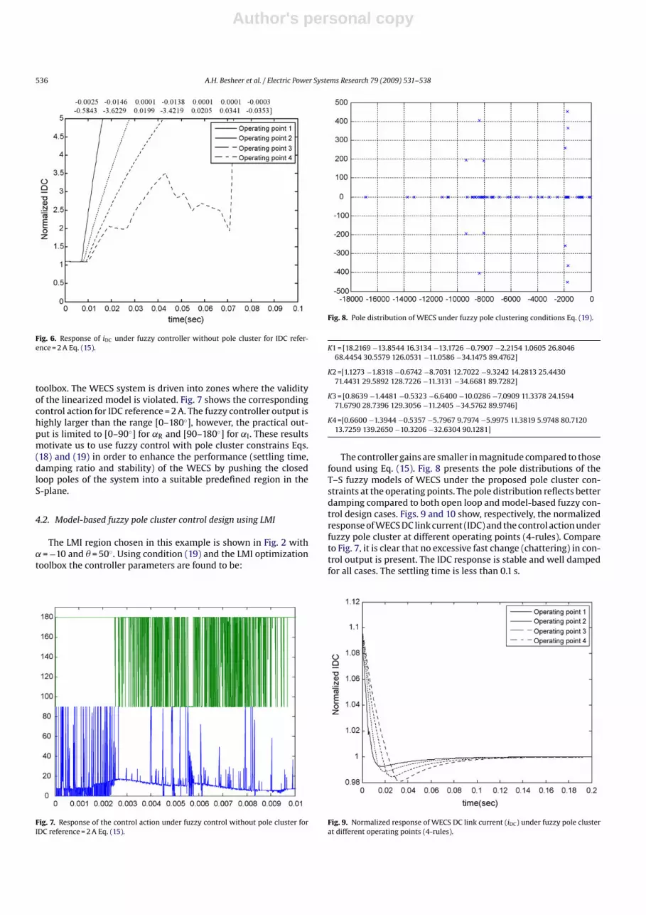
Fig. 6. Response of iDC under fuzzy controller without pole cluster for IDC refer-ence = 2 A Eq. (15).

toolbox. The WECS system is driven into zones where the validityof the linearized model is violated. Fig. 7 shows the correspondingcontrol action for IDC reference = 2 A. The fuzzy controller output ishighly larger than the range [0–180◦], however, the practical out-put is limited to [0–90◦] for ˛R and [90–180◦] for ˛I. These resultsmotivate us to use fuzzy control with pole cluster constrains Eqs.(18) and (19) in order to enhance the performance (settling time,damping ratio and stability) of the WECS by pushing the closedloop poles of the system into a suitable predefined region in theS-plane.

4.2. Model-based fuzzy pole cluster control design using LMI

The LMI region chosen in this example is shown in Fig. 2 with˛ = −10 and � = 50◦. Using condition (19) and the LMI optimizationtoolbox the controller parameters are found to be:

Fig. 7. Response of the control action under fuzzy control without pole cluster forIDC reference = 2 A Eq. (15).

Fig. 8. Pole distribution of WECS under fuzzy pole clustering conditions Eq. (19).

K1 = [18.2169 −13.8544 16.3134 −13.1726 −0.7907 −2.2154 1.0605 26.804668.4454 30.5579 126.0531 −11.0586 −34.1475 89.4762]

K2 =[1.1273 −1.8318 −0.6742 −8.7031 12.7022 −9.3242 14.2813 25.443071.4431 29.5892 128.7226 −11.3131 −34.6681 89.7282]

K3 = [0.8639 −1.4481 −0.5323 −6.6400 −10.0286 −7.0909 11.3378 24.159471.6790 28.7396 129.3056 −11.2405 −34.5762 89.9746]

K4 =[0.6600 −1.3944 −0.5357 −5.7967 9.7974 −5.9975 11.3819 5.9748 80.712013.7259 139.2650 −10.3206 −32.6304 90.1281]

The controller gains are smaller in magnitude compared to thosefound using Eq. (15). Fig. 8 presents the pole distributions of theT–S fuzzy models of WECS under the proposed pole cluster con-straints at the operating points. The pole distribution reflects betterdamping compared to both open loop and model-based fuzzy con-trol design cases. Figs. 9 and 10 show, respectively, the normalizedresponse of WECS DC link current (IDC) and the control action underfuzzy pole cluster at different operating points (4-rules). Compareto Fig. 7, it is clear that no excessive fast change (chattering) in con-trol output is present. The IDC response is stable and well dampedfor all cases. The settling time is less than 0.1 s.

Fig. 9. Normalized response of WECS DC link current (iDC) under fuzzy pole clusterat different operating points (4-rules).

Author's personal copy

A.H. Besheer et al. / Electric Power Systems Research 79 (2009) 531–538 537

Fig. 10. Response of the control action with fuzzy PDC pole cluster constrains forIDC reference = 2 A.

Fig. 11. The control system configuration.

4.3. PI control

In this section a simple PI controller is designed using frequencydomain optimization (Wiener-Hopf) procedures on the small signallinearized models as proposed by [16]. The PI gains Kp and Ki areso chosen as to minimize a performance index:

˝ = 12j�

j∞∫

−j∞

{E(s)˚1(s)E(−s) + U(s)˚2(s)U(−s)

}ds

Fig. 12. Dynamic response of WECS with PI controller to 10% disturbance in initialconditions.

where ˚1 and ˚2 are frequency-dependent weighting functions.Fig. 11 depicts the control system configuration considered for theoptimization procedures. Fig. 12 shows the dynamic response ofWECS under this controller. The PI controller is unable to achieve asettling time better than 0.3 s, which is triple the value achieved byfuzzy pole cluster controller. The IDC response in case of PI controlis more oscillatory compared to fuzzy pole cluster case. Comparingthe PI response (Figs. 11 and 12) with the fuzzy pole cluster response(Figs. 9 and 12), it is noticed that the response of closed loop sys-tem under fuzzy pole cluster approach exhibited a good dampingand fast recovery under initial condition perturbation over a wideoperating range. The control performance of the fuzzy pole clustersystem outperforms the PI control system.

5. Conclusion

In this paper, a model-based fuzzy control scheme is pro-posed to cope with the intrinsic non-linear behavior of WECS. TheTakagi–Sugeno fuzzy model is employed to approximate the non-linear model of WECS. Based on the fuzzy model, a fuzzy controlleris developed to guarantee not only the stability of fuzzy modeland fuzzy control system for the WECS but also control the tran-sient behavior of the system. Satisfactory time response and closedloop damping are achieved by forcing the closed loop poles into asuitable sub-region on the left half of the S-plane. The design pro-cedure is conceptually simple and natural. Moreover, the stabilityanalysis and control design problems are reduced to LMI problems.Therefore, they can be solved very efficiently in practice by convexprogramming techniques for LMI’s. Simulation results show thatthe proposed control approach exhibits a superior performance tothat of established traditional control methods.

Appendix A. List of symbols

B, J net friction and inertia of the rotating parts of the systemC self-excitation capacitanceidc, iqc peak d and q axes capacitor currentsiDC DC link currentidr, iqr peak rotor d and q axes currentsids, iqs peak stator d and q axes currentsis Rms stator currentLDC, RDC DC link inductance and resistanceLm magnetizing inductanceLr, Ls rotor and stator self inductancesN number of polesrr, rs rotor and stator resistancesvds, vqs peak stator d and q axes voltages

Greek symbols˛I INVERTER firing angle (90 ≤ ˛i ≤ 180◦)˛R converter firing angle (0 ≤ ˛R ≤ 90◦)ωe electrical frequency (rad/s)ωr shaft speed (rad/s)

References

[1] J.F. Manwell, J.G. McGowan, A.L. Rogers, Wind Energy Explained Theory, Designand Application, John Wiley & sons LTD, England, 2002.

[2] S.A. Delasaalle, D. Reardon, W.E. lLethead, M.J. Grimble, Review of wind turbinecontrol, Int. J. Control 52 (6) (1990) 1295–1310.

[3] A.H. Besheer, A linear Matrix Inequality Approach for Model Based Fuzzy Con-trol of Wind Energy Conversion System, Ph.D. dissertation, Electrical Power &Machines Department, Faculty of Engineering, Cairo University, Egypt, 2006.

[4] M.A. Mayosky, G.I.E. Cancelo, Direct adaptive control of wind energy conversionsystems using Gaussian network, IEEE Trans. Neural Netw. 10 (July (4)) (1999)898–906.

Author's personal copy

538 A.H. Besheer et al. / Electric Power Systems Research 79 (2009) 531–538

[5] T. Thiringer, J. Linders, Control by variable rotor speed of fixed pitch wind tur-bine operating in speed range, IEEE Trans. Energy Conversion 8 (September)(1993) 520–526.

[6] J. Tande, Exploitation of wind energy resources in proximity to weak electricgrids, in: Proceedings of the ENERGEX, Manama, 1998.

[7] H. De Battista, R. Mantz, C. Christiansen, Dynamical sliding mode power con-trol of wind driven induction generators, IEEE Trans. Energy Conversion 15(December) (2000) 451–457.

[8] H. De Battista, R.J. Mantz, Dynamical variable structure controller for powerregulation of wind energy conversion systems, IEEE Trans. Energy Conversion19 (December) (2004) 756–7563.

[9] S. Heier, W. Kleinkauf, Grid connection of wind energy converters, in: EuropeanCommunity Wind Energy Conference, Germany, March, 1993.

[10] K. Natarajan, A.M. Sharaf, S. Sivakumar, S. Naganathan, Modelling and con-trol design for wind energy conversion scheme using self-excited inductiongenerator, IEEE Trans. Energy Conversion September EC-2 (3) (1987) 506–512.

[11] R. Chedid, F. Mrad, M. Basma, Intelligent control of a class of wind energyconversion systems, IEEE Trans. Energy Conversion 14 (December (4)) (1999)1597–1604.

[12] H. Nakanishi, I.B. Turksen, M. Sugeno, A review and comparison of six reasoningmethods, Fuzzy Sets Syst. 57 (1993) 257–294.

[13] J. Ackermann, Robust Control: Systems with Uncertain Physical Parameters,Springer-Verlag, London, 1993.

[14] S. Boyd, L. El Ghaoui, E. Feron, V. Balakrishnan, Linear Matrix Inequalities inSystems and Control Theory, SIAM, PA, Philadelphia, 1994.

[15] G.L. Johnson, Wind Energy Systems, Prentice Hall Inc., Englewood Cliffs, NewJercy, 1985.

[16] R.M. Hilloowala, A.M. Sharaf, A utility interactive wind energy conversionscheme with an synchoronous DC link using a supplementary control loop,IEEE Trans. Energy Conversion 9 (September (3)) (1994) 558–563.

[17] T. Takagi, M. Sugeno, Fuzzy identification of systems and its applications tomodeling and control, IEEE Trans. Syst. Man Cybern. SMC-15 (January/February)(1985) 116–132.

[18] H.O. Wang, K. Tanaka, M.F. Griffin, An approach to fuzzy control of nonlinearsystems: Stability and design issues, IEEE Trans. Fuzzy Syst. 4 (February) (1996)14–23.

[19] H.O. Wang, K. Tanaka, M.F. Griffin, Parallel distributed compensation of non-linear systems by Takagi–Sugeno fuzzy model, in: Proceedings of the FuzzIEEELFES, vol. 95, 1995, pp. 531–538.

[20] H.O. Wang, K. Tanaka, M.F. Griffin, An analytical framework of fuzzy mod-eling and control of nonlinear systems: stability and design issues, WA, in:Proceedings of the Amer. Contr. Conf., Seattle, 1995, pp. 2272–2276.

[21] B.C. Kuo, Automatic Control Systems, Prentice-Hall, Englewood Cliffs, NJ,1982.

[22] M. Chilali, P. Gahinet, H∞ design with pole placement constraints: an LMIapproach, IEEE Trans. Automatic control 14 (March) (1996) 358–367.

[23] Yu. Nesterov, A. Nemirovsky, Interior Point Polynomial Methods in Convex Pro-gramming, SIMA, PA: Philadelphia, 1994.

[24] P. Gahinet, A. Nemirovski, A.J. Laub, M. Chilali, LMI Control Toolbox, The MathWorks, Natick, MA, 1995.