what types of neighbourhoods are redlined

Abstract This paper presents a case study of lending behaviour in the city ofRotterdam, the Netherlands. It shows what types of neighbourhoods areredlined by analyzing redlining data of the two largest suppliers of mortgageloans and comparing it to social-demographic and housing market data atthe neighbourhood level. Although this approach cannot explain redlining, itcan show which factors are related to lending behaviour. Low income,unemployment and ethnicity are strongly positively correlated to redlining.A discriminant analysis shows that the interaction between low income,unemployment or ethnicity on the one hand, and the average value of soldunits on the other hand can best approximate redlining. Lastly, this paper alsohighlights the importance of scale.

Keywords Credit Æ Discriminant analysis Æ Ethnic minorities ÆHomeownership Æ Housing market discrimination Æ Mortgage loans ÆNeighbourhood Æ Redlining Æ Rotterdam Æ The Netherlands

1 Introduction

In the mortgage finance market, the supply side (i.e. banks and other financialinstitutions) has the power to exclude part of the demand side (i.e. customers);

Manuel B. Aalbers formerly at: Amsterdam institute for Metropolitan and InternationalDevelopment Studies (AMIDSt), University of Amsterdam, Nieuwe Prinsengracht 130, 1018 VZAmsterdam, The Netherlands

M. B. Aalbers (&)Graduate School of Architecture, Planning and Preservation, Columbia University,New York City, NY, USAe-mail: [email protected]

123

J Housing Built Environ (2007) 22:177–198DOI 10.1007/s10901-007-9074-9

ART ICLE PO L IC Y AN D P R A CT I CE

What types of neighbourhoods are redlined?

Manuel B. Aalbers

Published online: 3 July 2007� Springer Science+Business Media B.V. 2007

one way of doing this is by redlining an area. Redlining is the process of notgranting mortgage loan applications from specific neighbourhoods. Manyauthors include uneven conditions such as higher transaction costs and higherinterest rates in their definition of redlining (e.g. Bradford and Marino 1977).The reason that financial institutions deny mortgage applications for certainneighbourhoods is that they have no trust in the financial feasibility of itscustomers or in the (future) value of the houses they inhabit (e.g. Jones andMaclennan 1987; Schill and Wachter 1994). They expect real estate prices tobe falling (Kantor and Nystuen 1982; Lang and Nakamura 1993). The risk thata homeowner can only sell a house for a lower price than s/he bought it for,and as a result cannot pay off the mortgage, is considered too big. Banksassume that members of certain social-economic or ethnic groups are, onaverage, less able to fulfil their financial commitments (Aalbers 2005c; Rossand Yinger 2002). Redlining in the mortgage market strikes low-incomeneighbourhoods and ethnic-minority neighbourhoods in particular. Yet,redlining not only strikes low-income families and ethnic minorities, but alsoeveryone else applying for a mortgage in a redlined neighbourhood. Redliningis not a form of individual-based exclusion, but a form of place-based socialexclusion (Aalbers 2005b; Gregory 1998).

This paper will first discuss the literature on redlining. The subsequentsections will discuss the current study which answers the question: what typesof neighbourhoods are redlined? This study makes use of an earlier study onthe city of Rotterdam that demonstrates the existence of redlining (Aalbers2003, 2005a, b). Rather than presenting evidence of redlining, this paper willshow what the social-economic and housing market characteristics of redlinedneighbourhoods are. It demonstrates the relevance of some of the assump-tions of the literature and disaffirms the relevance of others.

2 Previous research on redlining

Most research on redlining comes from the United States, although some of ithas also been carried out in South Africa (e.g. Kotze and Huyssteen 1990),Canada (e.g. Murdie 1986; Harris and Forrester 2003), Australia (e.g. Engels1994), and the United Kingdom (e.g. Boddy 1976; Williams 1978; Jones andMaclennan 1987). The earliest examples date from the 1930s, but in the US itwas only perceived as a national urban problem in the 1970s when community-based organizations all over the country exposed redlining practices (for anoverview, see Squires 1992). The US government responded by implementingthe Home Mortgage Disclosure Act (HMDA) in 1975, and the CommunityReinvestment Act (CRA) in 1977. The first requires lenders to report grantedloans by census tract; the second requires lenders to provide credit to the localcommunities within the states in which they are active. Since 1990, the HMDAalso requires banks to report the race and income of all mortgage loanapplicants.

178 M. B. Aalbers

123

The question is, why do banks consider certain neighbourhoods as ‘badrisks’? Or, in other words, what constitutes ‘bad risk neighbourhoods’? Whichtypes of neighbourhoods are redlined? The literature on redlining has oftenfocused on redlined neighbourhoods as ethnic-minority neighbourhoods(King 1980; Schafer and Ladd 1981; Kotze and Huyssteen 1990; Schill andWachter 1994; Tootell 1996; Phillips-Patrick and Rossi 1996; Reibel 2000;Ross and Yinger 2002: 39), but alternative explanations see redlining as aresult of low demand and related uncertainty (Jones and Maclennan 1987;Lang and Nakamura 1993), low housing prices (Kantor and Nystuen 1982;Lang and Nakamura 1993), or bad experiences of banks such as high defaultrates or other types of risk (Jones and Maclennan 1987; Berkovec et al. 1994;Schill and Wachter 1994; Hunter and Walker 1996; Tootell 1996). Others haveclaimed banks redline neighbourhoods because banks consider poverty toohigh or the average income of the current residents too low (Dymski andVeitch 1994; Schill and Wachter 1994; Tootell 1996; Margulis 1998; Ross andTootell 2004; Reibel 2000), because dwellings are too old and maintenancelimited (Margulis 1998), or because the share of owner-occupied homes isconsidered too low and the share of rented housing too large (Kantor andNystuen 1982). Low demand is often directly related to a low share of owner-occupied units; as Lang and Nakamura (1993) argue, the probability of loandenial for applications to finance home purchases in a particular neighbour-hood should decline as the number of house sales in that neighbourhood goesup. This is because it may be hypothesized that redlining occurs due to a lackof comparable properties in the neighbourhood, and that consequentlyinvestment may be considered too risky.

Some of the earliest studies found evidence of redlining (Ahlbrandt 1977;Hutchinson et al. 1977; Schafer 1978), but have been criticized for omittingimportant variables and for the use of aggregate level data (see Murdie 1986;Dymski 2006). Bradbury et al. (1989) and Shlay (1989) have showed thatminority and inner-city neighbourhoods receive less credit, but Dymski (2006)suggests that the problem of this approach is that it is susceptible to thecriticism of pre-selection bias. King (1980) and Phillips-Patrick and Rossi(1996) find that the probability of loan denial is higher in ethnic minority areasthan in majority white areas, but cannot show the existence of redlining.Schafer and Ladd (1981) do show the existence of redlining, but they alsoshow that it is not a widespread phenomenon. Kotze and Huyssteen (1990)apply discriminant analysis to show the existence of redlining practices inCape Town, South Africa. Also, the US studies of Kantor and Nystuen (1982),Dedman in his Pulitzer Price winning series of articles (1988), Dymski andVeitch (1994) and Reibel (2000) as well as the UK studies of Boddy (1976)and Williams (1978) and the Australian study of Engels (1994), show theevidence or likeliness of redlining, but Kantor and Nystuen (1982) andDymski and Veitch (1994) admit that their results leave room for alternative,yet less plausible, conclusions. Recent US studies by Schill and Wachter(1994), Tootell (1996), Hunter and Walker (1996), and Margulis (1998) find noevidence of redlining. A default rates study by Berkovec et al. (1994) does not

What types of neighbourhoods are redlined? 179

123

find evidence of redlining, but this approach has been heavily criticized bymany authors, including prominent housing discrimination researchers such asRoss et al. (1996; Ross and Yinger 2002) who argue that the default approachis not only full of bias and based on the wrong assumptions (see also Bradfordand Shlay 1996), but also that it cannot isolate the impact of prejudice-basedor any other type of discrimination on loan performance. Finally, Ross andTootell (2004) do find evidence of redlining, but the probability of denial isnot higher in ethnic-minority neighbourhoods, suggesting that there otherfactors are more important such as a high concentration of low-incomehouseholds.

In conclusion, it is fair to say that while few would deny the existence ofhistoric redlining in the US, recent evidence of redlining is scarce. Today,redlining in the US is less likely to take place because it is prohibited andbanks have to make their lending data available for research. In addition,changes in financial markets have made it more likely that lenders will chargehigher interest rates and closing fees in high-risk areas rather than that red-lining will occur in these areas. Yet, we cannot simply conclude that redliningno longer exists in the US. Indeed, researchers who demonstrate the existenceof redlining practices can be easily accused of omitting variables. At the sametime, researchers who demonstrate the non-existence of redlining can becriticized on the same grounds but also for not taking most of the lendingprocess into account—for instance by ignoring pre-application denials (e.g.Ross and Yinger 2002). Moreover, a great deal of research has left out the‘geographically contingent nature of discrimination’ (Holloway 1998) and hasoverlooked the fact that lenders can easily adjust their spatial lending policies.Since redlining is measured on the district level, they can engage in cherry-picking behaviour by redlining part of a district as long as they grant mort-gages in other parts. In addition, most models used to demonstrate the (non-)existence of redlining do not provide an explanation of de facto or actualredlining (cf. Nesiba 1996). Indeed, recent redlining research in the US hasmostly focused on abstract models and on prediction of redlining, not on thediscovery and explanation of redlining (Aalbers 2005a; Hillier 2003; but seeImmergluck 2004 and Squires, 1992 for studies that have focused on the socialand legal battles fought on redlining).

3 Research design

The current study focuses on actual or de facto redlining (cf. Kantor andNystuen 1982) in the Netherlands. It has been established in preceding studiesthat redlining took place in the late 1990s in the city of Rotterdam (Aalbers2003, 2005a, b). This paper uses the lending data gathered in these earlierstudies and shows which types of neighbourhoods are redlined by comparingthat lending data to other data on the city of Rotterdam. Both the primarydata on lending and the secondary data from the Rotterdam Centre forResearch and Statistics (COS) are neighbourhood-level data. The first makes

180 M. B. Aalbers

123

use of postcodes, the second of ‘neighbourhood combinations’. There is al-most a perfect fit between these two types of neighbourhood data becauseneighbourhood combinations are usually the same as postcode data on thefour-position level (comparable to the US 5-digit numeric ZIP codes). Withsome minor alterations these two types of data can easily be analyzed withinthe same framework. In addition, this study also makes use of interviews withreal estate agents and mortgage intermediaries.

In the literature, it is argued that redlining can have several causes andtherefore be related to different variables. Some argue that redlining is a signof racial discrimination; therefore data on ethnicity have been included.Others have argued that redlining takes place because lenders avoid low-income areas, areas with predominantly rental dwellings or low housing valueareas because of the low rate of return; therefore, data on income, unem-ployment, tenure and housing value have been included. Often it is also ar-gued that lenders exclude areas because of lack of knowledge; this is anotherreason for including tenure, but it is also a reason for including the number ofunits sold by NVM real estate agents. Given the small number of sold unitsper neighbourhood (in absolute terms), lenders may be faced with a lack ofmarket knowledge, which may induce them to redline such areas: for lenders,a lack of information is just as bad as negative information. Yet others look atthe state of the housing stock and argue that areas may be redlined because ofthe predominance of old dwellings (a variable on building period has beenincluded) or of high turnover rates, vacancy rates and crime, all of which maysignify downgrading (variables on length of residence, vacancy, safety andcrime have been included). Mortgage loan default rates by neighbourhoodwere not available. For some variables, averages per neighbourhood havebeen used (e.g. income); for other variables we have used the differentstatistical groups as provided by COS (e.g. building period). All thesevariables refer to either 1999 or 2000. In this particular step of the researchdesign we do not take the problem of within-neighbourhood differences intoaccount because the redlining evidence this study builds on clearly shows thatbanks have also ignored these differences. Since we are trying to relate pat-terns of lending behaviour to other neighbourhood characteristics, thesedifferences have to be ignored.

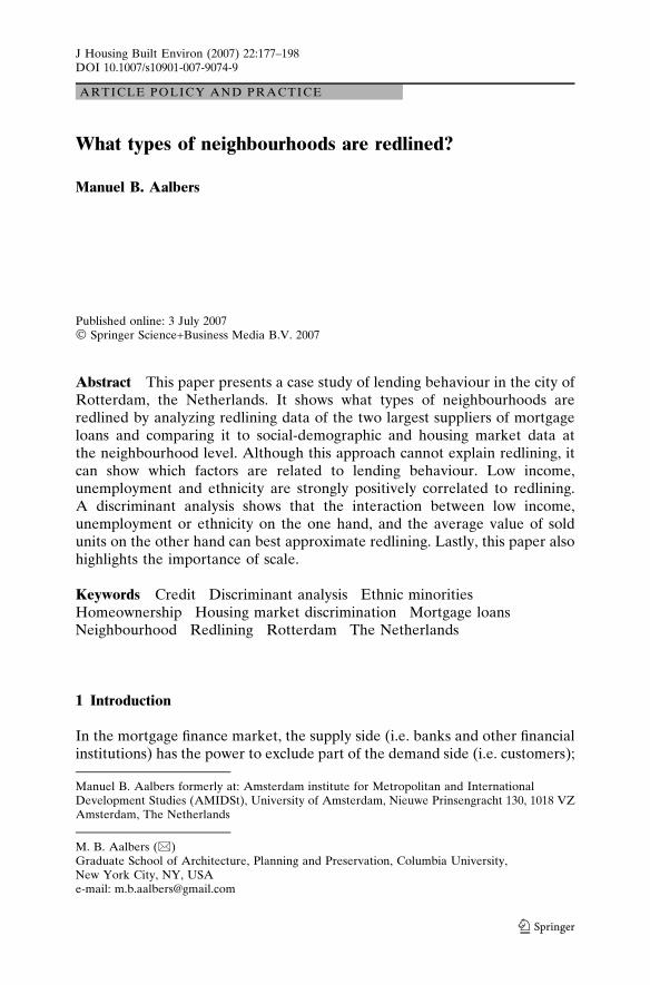
The lending data on the postcode level were collected in earlier studiescarried out between 1999 and 2003 (Aalbers 2003, 2005a, b; see Fig. 1). Thesestudies report the situation in the second half of 1999 and are based on thelending behaviour data of the two largest suppliers of mortgage loans inRotterdam (two large Dutch general banks). Even though these banks havechanged their redlining policies several times, they had almost identicalredlining policies at the end of 1999. We here use the actual fourfold divisionused by these two banks at the end of 1999. The first reads ‘‘mortgages grantedup to 125 per cent of estimated execution value’’ and is called ‘greenlining’.The second reads ‘‘mortgages granted up to 70 or 80 per cent of estimatedexecution value’’ (first bank) or ‘‘mortgages granted on a case-by-case basis’’(second bank); we have dubbed this ‘yellowlining’ (yellowlining has often


123

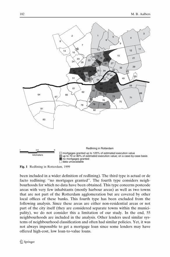
been included in a wider definition of redlining). The third type is actual or defacto redlining: ‘‘no mortgages granted’’. The fourth type considers neigh-bourhoods for which no data have been obtained. This type concerns postcodeareas with very few inhabitants (mostly harbour areas) as well as two townsthat are not part of the Rotterdam agglomeration but are covered by otherlocal offices of these banks. This fourth type has been excluded from thefollowing analysis. Since these areas are either non-residential areas or notpart of the city itself (they are considered separate towns within the munici-pality), we do not consider this a limitation of our study. In the end, 55neighbourhoods are included in the analysis. Other lenders used similar sys-tems of neighbourhood classification and often had similar policies. Yet, it wasnot always impossible to get a mortgage loan since some lenders may haveoffered high-cost, low loan-to-value loans.

0 2.5 5

kilometers

50

57

10

76

123

456

7

89

11121314

15

16

17

181920 21

2223

2425

26 2728

29

30 31

3233

34353637 38394041 42

43 4445 4647

484951 5253

54 5556

5859

60

61

62

63

64

65

6667

68

69 70

71

7273

74

7577

78 79 80

8182

83

Redlining in Rotterdam

mortgages granted up to 125% of estimated execution valueup to 70 or 80% of estimated execution value; on a case-by-case basisno mortgages granteddata unvavailable

Fig. 1 Redlining in Rotterdam, 1999

182 M. B. Aalbers

123

For these neighbourhoods, we first calculated a Spearman correlation be-tween lending behaviour on the one hand, and all other individual variableson the other hand. In the next step—following Press and Wilson’s (1978)‘guide to discriminant analysis’—we did not include all variables. We onlyincluded those with highest correlations and, of those, a maximum of twovariables per indicator; all of these variables are two-tailed significant at the0.01 level. This yields a list of four group-related variables (on income andrace) and four housing-related variables (on tenure, information and value).Subsequently, the correlations between all these four-plus-four individualvariables were computed. For the next round of analysis, all correlations over0.75 were excluded. This was necessary because correlations between twovariables over 0.75 (high, or near perfect, multicollinearity) do not properlyenable a higher percentage of cases accurately predicted in the next round ofanalysis; they are too correlated to include their interaction. (Multicollinearityoccurs when two or more ‘predictor variables’ are themselves highly corre-lated. Removing one of these variables, or their interaction in the model, mayreduce or eliminate multicollinearity.)

Next, a series of discriminant analyses were undertaken between, eachtime, one of the group-related variables (‘predictor variable 1’), one of thehousing-related variables (‘predictor variable 2’), and lending behaviour as the‘dependent variable’. With the help of Wilks’ lambda test of significance, acanonical correlation analysis and a factor structure matrix, we account for thepercentage of cases of lending behaviour accurately predicted through theinteraction of two predictor variables. Since this resulted in a very high per-centage of cases accurately predicted, it was decided not to compute a modelwith three or more independent variables. Moreover, this would be almostimpossible because of the resulting high degree of multicollinearity.

Discriminant analysis was selected because it can be used to determinewhich continuous variables discriminate between a number of empiricallyobserved groups, but also because it has been applied in the redlining study byKotze and Huyssteen (1990). Discriminant function analysis, also known asmultiple discriminant analysis, was preferred over multivariate analysis ofvariance because the latter models the groups as independent variables or‘predictors’. Although logistic regression is often considered superior to dis-criminant analysis, the latter is to be preferred when the assumptions ofmultivariate normality are met (or are irrelevant because no sample is used),and when the dependent variable is ordinal (Press and Wilson 1978). Commonproblems with discriminant analysis are related to sample size and outliers,but since this study does not use a sample, these problems were irrelevant.Considering the high percentage of cases accurately predicted, outliers wererelatively close to the cases.

The next and final step in the analysis considers outliers. Rather thanexcluding outliers to get a clearer picture of a correlation or equation, wedecided to focus on these outliers because the study of outliers can teach usmore about what types of neighbourhoods are redlined. The basic idea is thatwe look at which neighbourhoods have the qualities of a redlined neigh-


123

bourhood but are not redlined, or which neighbourhoods have the qualities ofa greenlined neighbourhood but are not greenlined. We have done this withthe help of hierarchical and k-means cluster analyses. In a number of roundswe have selected (1) all variables, (2) the four-plus-four variables, (3) twovariables (‘ethnic minorities’ and ‘average value of sold dwellings’ since theseshowed the highest percentage of cases accurately predicted in the discrimi-nant analysis) for both types of cluster analyses and for different sizes ofclusters. Subsequently, we have compared these clusters to the lendingbehaviour data per postcode area. For example, a neighbourhood that scoreshigh on variables such as ethnic minorities and unemployment, and low onincome and value of dwellings, can be expected to be a redlined neighbour-hood because most redlined neighbourhoods have these qualities. If, however,a neighbourhood showing the qualities of a redlined neighbourhood is notredlined, it is an outlier.

4 Results

4.1 Correlations

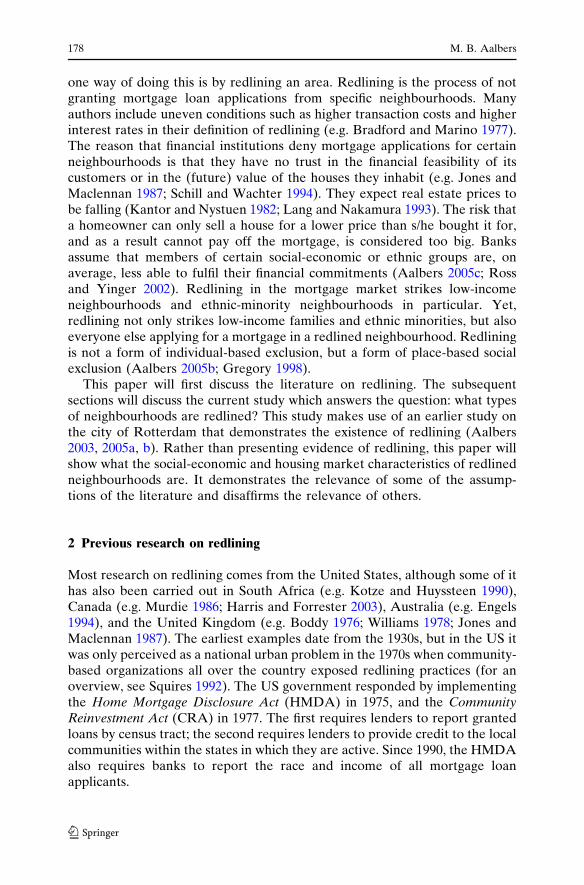
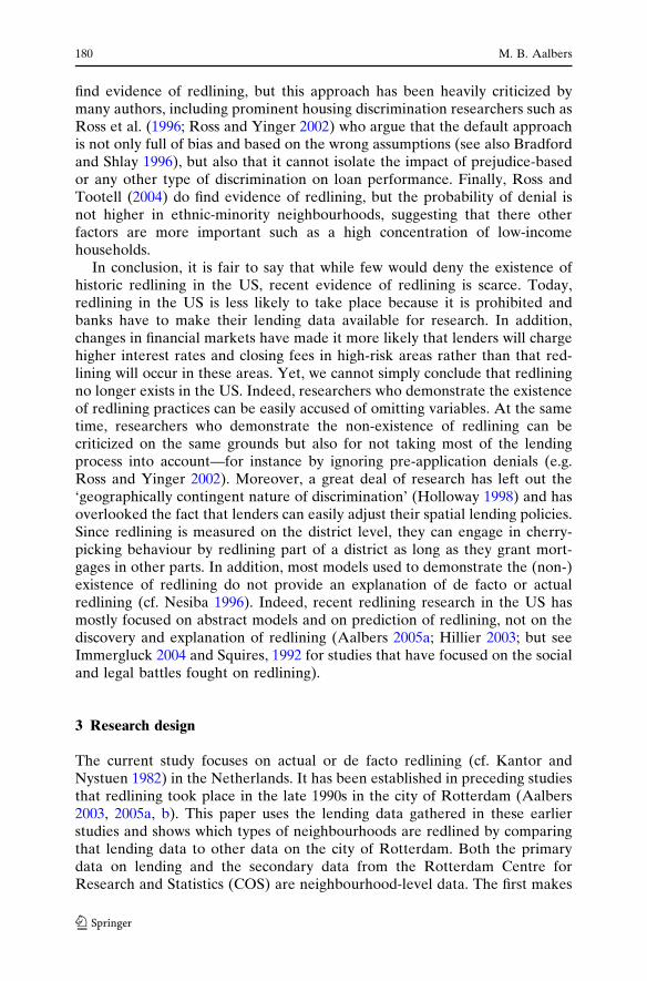
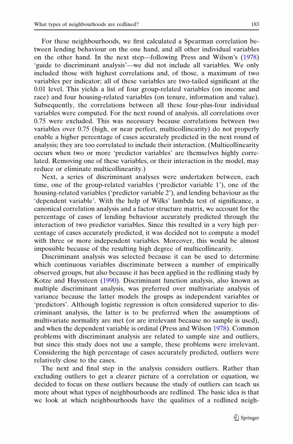
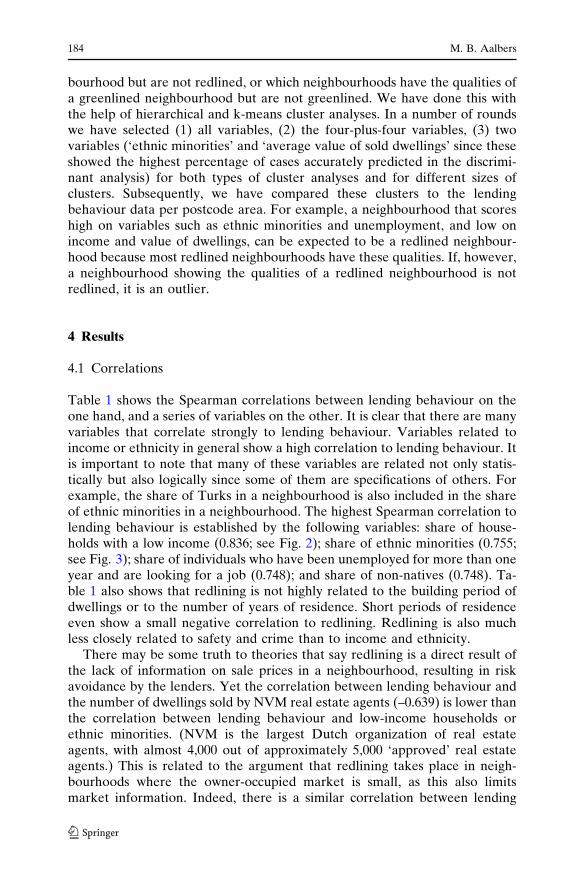
Table 1 shows the Spearman correlations between lending behaviour on theone hand, and a series of variables on the other. It is clear that there are manyvariables that correlate strongly to lending behaviour. Variables related toincome or ethnicity in general show a high correlation to lending behaviour. Itis important to note that many of these variables are related not only statis-tically but also logically since some of them are specifications of others. Forexample, the share of Turks in a neighbourhood is also included in the shareof ethnic minorities in a neighbourhood. The highest Spearman correlation tolending behaviour is established by the following variables: share of house-holds with a low income (0.836; see Fig. 2); share of ethnic minorities (0.755;see Fig. 3); share of individuals who have been unemployed for more than oneyear and are looking for a job (0.748); and share of non-natives (0.748). Ta-ble 1 also shows that redlining is not highly related to the building period ofdwellings or to the number of years of residence. Short periods of residenceeven show a small negative correlation to redlining. Redlining is also muchless closely related to safety and crime than to income and ethnicity.

There may be some truth to theories that say redlining is a direct result ofthe lack of information on sale prices in a neighbourhood, resulting in riskavoidance by the lenders. Yet the correlation between lending behaviour andthe number of dwellings sold by NVM real estate agents (–0.639) is lower thanthe correlation between lending behaviour and low-income households orethnic minorities. (NVM is the largest Dutch organization of real estateagents, with almost 4,000 out of approximately 5,000 ‘approved’ real estateagents.) This is related to the argument that redlining takes place in neigh-bourhoods where the owner-occupied market is small, as this also limitsmarket information. Indeed, there is a similar correlation between lending

184 M. B. Aalbers

123

behaviour and the share of owner-occupied dwellings in a neighbourhood(–0.636). Along the same lines, one could argue that redlining is related to theaverage value of owner-occupied dwellings, as lenders may find lower-priceddwellings less profitable. Again, there is a negative correlation betweenlending behaviour on the one hand, and both the average value of sold units

Table 1 Spearman correlations between ‘independent variables’ and lending behaviour, orderedfrom highest to lowest correlation

Variable Lending behaviour

Income: % households with a low income 0.836**Race: % ethnic minorities 0.755**Income: % persons more than 1 year not working

and looking for work compared to potential labour force0.748**

Race: % non-natives 0.748**Income: % persons more than 3 years on social

security compared to potential labour force0.746**

Race: % Turks 0.744**Value: average value owner-occupied dwellings –0.738**Race: Moroccans 0.713**Income: standardized household income (NL = 100) –0.704**Income: % households with a high income –0.660**Race: % Surinamese 0.644**Information: number of dwellings sold by NVM real estate agents –0.639**Value: average value of sold units –0.636**Tenure: % owner-occupied dwellings –0.636**Value: % value owner-occupied dwellings lower than 50,000 guilders 0.635**Safety: safety index (per neighbourhood) –0.509**Value: % value owner-occupied dwellings 100,000–150,000 guilders –0.507**Value: % value owner-occupied dwellings more than 150,000 guilders –0.502**Turnover: % residence at address 5–9 years 0.501**Value: % value owner-occupied dwellings 75,000–100,000 guilders –0.498**Tenure: % social rented dwellings 0.484**Turnover: % residence at address more than 15 years –0.468**Building period: % dwellings built 1960–1969 –0.458**Safety: intimidation and violence (% victims) 0.445**Building period: % dwellings built 1906–1930 0.424**Turnover: % residence at address 10–14 years 0.307*Building period: % dwellings built 1970–1979 –0.274*Building period: % dwellings built after 1990 0.272*Vacancy: administrative vacancies (number of dwellings) 0.231Safety: pickpockets (% victims) 0.198Safety: (attempted) burglary (% victims) 0.196Tenure: % private rented dwellings –0.181Building period: % dwellings built before 1906 0.153Turnover: % residence at address 2–4 years 0.127Building period: % dwellings built 1945–1959 –0.116Turnover: % residence at address less than 1 year –0.110Building period: % dwellings built 1980–1989 –0.110Value: % value owner-occupied dwellings

50,000–75,000 guilders–0.105

Building period: % dwellings built 1931–1944 –0.051Turnover: % residence at address 1 year –0.022

*Significant at the 0.05 level

**Significant at the 0.01 level


123

per neighbourhood (–0.636) and the average value of owner-occupied dwell-ings in the neighbourhood (–0.738) on the other hand. In other words, thesehousing-related variables (on information, value and tenure) are significantlycorrelated to lending behaviour, but less so than group-related variables(income, race).

4.2 Discriminant analysis

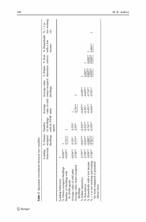
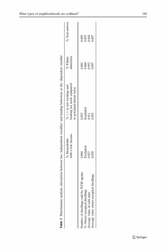
As explained in Sect. 3, eight variables have been selected for discriminantanalysis. In Table 2 one can see the Spearman correlations between all ninevariables (including redlining). Correlations between variables over 0.75 havebeen excluded from two-variable-interaction discriminant analysis for reasonsof multicollinearity; in Table 2, these correlations are underlined. Table 3shows the results of the variables included in the discriminant analysis as well

0 2.5 5

kilometers

68

82

55

48

13

50

33

10

16

76

123

456

7

89

111214

1517

181920

212223

2425

26 2728

29

30 31

32343536

37 38394041 4243 4445 46

47

4951 52535456

5758

5960

61

62

63

64

65

6667

69 70

71

7273

74

7577

78 79 80

81

83

Households with a low income

7 - 20%21 - 29%32 - 40%data unavailable

Fig. 2 Households with a low income in Rotterdam, 1999

186 M. B. Aalbers

123

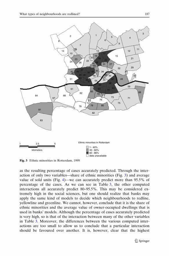
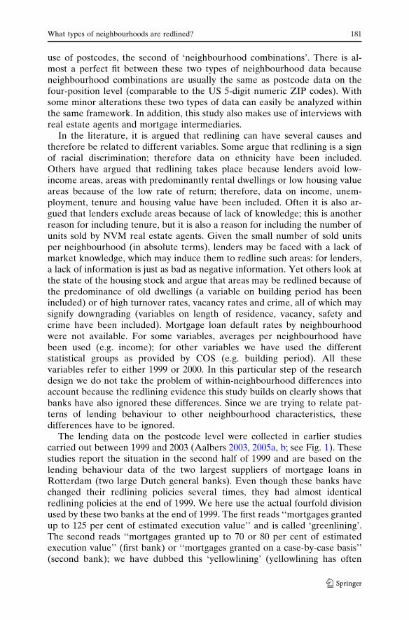
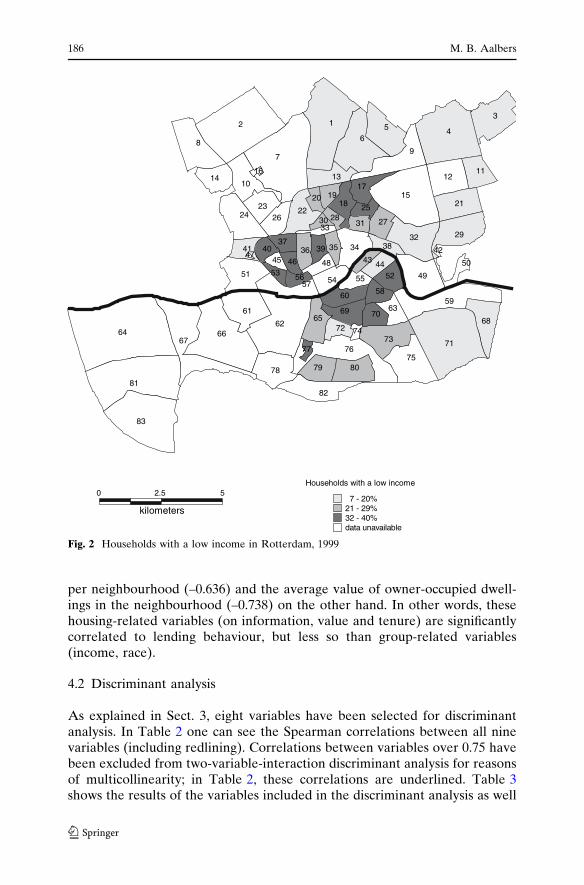
as the resulting percentage of cases accurately predicted. Through the inter-action of only two variables—share of ethnic minorities (Fig. 3) and averagevalue of sold units (Fig. 4)—we can accurately predict more than 95.5% ofpercentage of the cases. As we can see in Table 3, the other computedinteractions all accurately predict 80–95.5%. This may be considered ex-tremely high in the social sciences, but one should realize that banks mayapply the same kind of models to decide which neighbourhoods to redline,yellowline and greenline. We cannot, however, conclude that it is the share ofethnic minorities and the average value of owner-occupied dwellings that isused in banks’ models. Although the percentage of cases accurately predictedis very high, so is that of the interaction between many of the other variablesin Table 3. Moreover, the differences between the various computed inter-actions are too small to allow us to conclude that a particular interactionshould be favoured over another. It is, however, clear that the highest

0 2.5 5

kilometers

68

82

55

48

13

50

33

10

16

76

123

456

7

89

111214

1517

1819

20 2122

2324

2526

2728

29

30 31

323435

3637 38394041 42

43 4445 4647

4951 52535456

5758

5960

61

62

63

64

65

6667

69 70

71

7273

74

7577

78 79 80

81

83

Ethnic minorities in Rotterdam

1 - 40%40 - 60%60 - 86%data unavailable

Fig. 3 Ethnic minorities in Rotterdam, 1999


123

Ta

ble

2S

pe

arm

an

corr

ela

tio

ns

be

twee

ntw

ov

ari

ab

les

Len

din

gb

eh

av

iou

r%

Ow

ner

-o

ccu

pie

dd

we

llin

gs

Nu

mb

er

of

dw

ell

ing

sso

ldb

yN

VM

ag

en

ts

Av

era

ge

va

lue

of

sold

un

its

Av

era

ge

va

lue

ow

ne

r-o

ccu

pie

dd

we

llin

gs

%E

thn

icm

ino

riti

es

%N

on

-n

ati

ve

s%

Ho

use

ho

lds

wit

ha

low

inco

me

%>

1y

rn

ot

wo

rkin

ge

tc.

Le

nd

ing

be

ha

vio

ur

1%

Ow

ner

-occ

up

ied

dw

ell

ing

s–

0.6

36

**

1N

um

be

ro

fd

we

llin

gs

sold

by

NV

Ma

ge

nts

–0

.63

9*

*0

.75

2*

*1

Av

era

ge

va

lue

of

sold

un

its

–0

.63

6*

*0

.35

5*

0.3

25*

1A

ve

rag

ev

alu

eo

wn

er-

occ

up

ied

dw

ell

ing

s0

.738

**

0.5

75

**

0.5

57*

0.7

76

**

1

%E

thn

icm

ino

riti

es0

.755

**

–0

.61

7*

*–

0.5

18

**

–0

.40

7*

*–

0.6

28

**

1%

No

n-n

ati

ve

s0

.748

**

–0

.61

4*

*–

0.5

32

**

–0

.38

1*

–0

.62

9*

*0

.965

**

1%

Ho

use

ho

lds

wit

ha

low

inco

me

0.8

36*

*–0

.89

8*

*–

0.7

41

**

–0

.45

1*

*–

0.7

18

**

0.8

63*

*0

.85

8*

*1

%>

1y

rn

ot

wo

rkin

ga

nd

loo

kin

gfo

rw

ork

com

pa

red

top

ote

nti

al

lab

ou

rfo

rce

0.7

48*

*–0

.76

1*

*–

0.5

59

**

–0

.43

4*

*–

0.7

01

**

0.8

59*

*0

.82

0*

*0

.964

**

1

188 M. B. Aalbers

123

Ta

ble

3D

iscr

imin

an

ta

na

lysi

s,in

tera

ctio

nb

etw

een

two

‘in

de

pe

nd

en

tv

ari

ab

les’

an

dle

nd

ing

be

ha

vio

ur

as

the

‘de

pe

nd

en

tv

ari

ab

le’

%H

ou

seh

old

sw

ith

alo

win

com

e%

>1

yr

no

tw

ork

ing

an

dlo

ok

ing

for

wo

rkco

mp

are

dto

po

ten

tia

lla

bo

ur

forc

e

%E

thn

icm

ino

riti

es

%N

on

-na

tiv

es

Nu

mb

er

of

dw

ell

ing

sso

ldb

yN

VM

ag

en

ts0

.804

0.8

53

0.8

610

.849

%O

wn

er-

occ

up

ied

dw

ell

ing

sE

xcl

ud

ed

Ex

clu

de

d0

.864

0.8

55A

ve

rag

ev

alu

eo

fso

ldu

nit

s0

.927

0.9

11

0.9

520

.944

Av

era

ge

va

lue

ow

ne

r-o

ccu

pie

dd

we

llin

gs

0.8

280

.85

50

.897

0.8

97


123

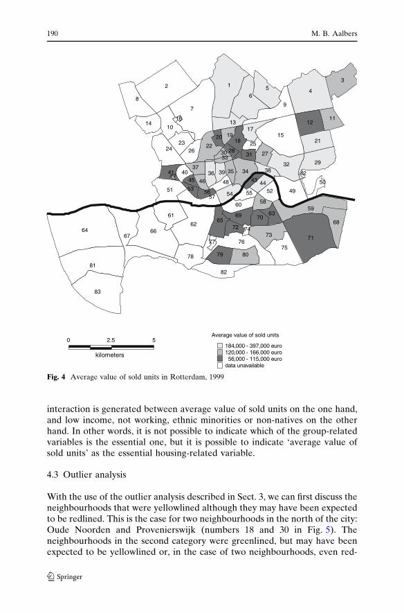
interaction is generated between average value of sold units on the one hand,and low income, not working, ethnic minorities or non-natives on the otherhand. In other words, it is not possible to indicate which of the group-relatedvariables is the essential one, but it is possible to indicate ‘average value ofsold units’ as the essential housing-related variable.

4.3 Outlier analysis

With the use of the outlier analysis described in Sect. 3, we can first discuss theneighbourhoods that were yellowlined although they may have been expectedto be redlined. This is the case for two neighbourhoods in the north of the city:Oude Noorden and Provenierswijk (numbers 18 and 30 in Fig. 5). Theneighbourhoods in the second category were greenlined, but may have beenexpected to be yellowlined or, in the case of two neighbourhoods, even red-

0 2.5 5

kilometers

68

82

55

48

13

50

33

10

16

76

123

456

7

89

111214

1517

181920

212223

2425

26 2728

29

30 31

32343536

37 38394041 4243 4445 46

47

4951 52535456

5758

5960

61

62

63

64

65

6667

69 70

71

7273

74

7577

78 79 80

81

83

Average value of sold units

184,000 - 397,000 euro120,000 - 166,000 euro56,000 - 115,000 euro

data unavailable

Fig. 4 Average value of sold units in Rotterdam, 1999

190 M. B. Aalbers

123

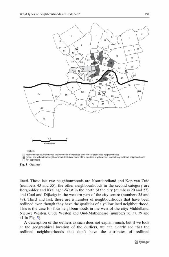
lined. These last two neighbourhoods are Noordereiland and Kop van Zuid(numbers 43 and 55); the other neighbourhoods in the second category areBergpolder and Kralingen-West in the north of the city (numbers 20 and 27),and Cool and Dijkzigt in the western part of the city centre (numbers 35 and48). Third and last, there are a number of neighbourhoods that have beenredlined even though they have the qualities of a yellowlined neighbourhood.This is the case for four neighbourhoods in the west of the city: Middelland,Nieuwe Westen, Oude Westen and Oud-Mathenesse (numbers 36, 37, 39 and41 in Fig. 5).

A description of the outliers as such does not explain much, but if we lookat the geographical location of the outliers, we can clearly see that theredlined neighbourhoods that don’t have the attributes of redlined

0 2.5 5

kilometers

68

82

55

48

13

50

33

10

16

76

123

456

7

89

111214

1517

181920 21

2223

2425

26 2728

29

30 31

32343536

37 38394041 4243 4445 46

47

4951 52535456

5758

5960

61

62

63

64

65

6667

69 70

71

7273

74

7577

78 79 80

81

83

Outliers

not applicable

redlined neighbourhoods that show some of the qualities of yellow- or greenlined neighbourhoodsgreen- and yellowlined neighbourhoods that show some of the qualities of yellowlined, respectively redlined, neighbourhoods

Fig. 5 Outliers


123

neighbourhoods are all located in the western part of the city and are situatedadjacent to other redlined neighbourhoods. We can also see that green-lined and yellowlined neighbourhoods that have the qualities of yellow-lined respectively redlined neighbourhoods are located north of the centre, inthe western part of the city centre or directly south of the river Maas.

Now we have to explain why these neighbourhoods are outliers. We do thatin two ways: first, through an individual neighbourhood assessment; and sec-ond, by looking at the scale of lending behaviour patterns. To start with theneighbourhood Kop van Zuid (55; not including the Kop van Zuid-Entrepotneighbourhood), it is not surprising that it is greenlined and not yellowlined orredlined. In 1999 (to which the data apply), this area was starting to beredeveloped from a site of brownfields to a neighbourhood with mostlyexpensive housing in addition to some offices and recreational facilities. Forthe Kop van Zuid the statistics showed a bleaker picture than the futureperspectives. Adjacent Noordereiland (43), an island between the north andsouth banks of the river Maas, is largely a low to middle income residentialarea. But its proximity to both the city centre and the redeveloping Kop vanZuid area as well as its situation on the water and related possibilities forupgrading make it a possibly attractive location.

Just on the other side of the river, the Dijkzigt (48) neighbourhood (namedafter the hospital with the same name) may have a very small owner-occupiedsector (2.5%); there is no information on sold dwellings or average shares ofethnic minorities and non-natives. It is also a well-situated neighbourhood,lying on the edge of the city centre next to the museum district. Its few owner-occupied dwellings show the highest average value of the city; thus, it is notvery surprising that the neighbourhood is not yellowlined but greenlined. Nextto Dijkzigt we find the Cool (35) neighbourhood, which is the western part ofthe city centre. Although the statistics show that it is the poorest part of thecity centre, its central location makes it an attractive area, as indicated by thefact that the increase in house prices between 1999 and 2004 was bigger thanelsewhere in the city.

To explain why the other neighbourhoods mentioned above are notredlined (respectively yellowlined) while other statistics suggest they have thequalities of a redlined (respectively yellowlined) area, as well as to explainwhy some other neighbourhoods are redlined while they have the qualities ofa yellowlined area, we have to look at the scale of green-, yellow- and red-lining. Like the above-mentioned Oude Noorden and Provenierswijk neigh-bourhoods, the Bergpolder (20) and Kralingen-West (27) neighbourhoods arelocated in the north of the city. They both benefit from the fact that adjacentneighbourhoods are predominantly greenlined. Kralingen-West has a goodname: together with the much richer and more expensive Kralingen-Eastneighbourhood it forms the district of Kralingen. In the discourse of good andbad areas in Rotterdam, Kralingen is said to be one of the best, if not the verybest area of the city. Kralingen-West, however, has above-average shares ofethnic minorities, non-natives and low-income households, but an above-average housing value. Both Bergpolder and Kralingen-West have a mix of

192 M. B. Aalbers

123

the qualities of yellowlined and greenlined areas, but their location in the city(in the north, bordering mostly greenlined areas) provides them with a rela-tively favourable position.

As one can clearly see in Fig. 1, redlined areas are predominantly locatedwest and south of the city centre. The neighbourhoods redlined there are thusadjacent to other redlined neighbourhoods. Even though some of theseneighbourhoods may not have the statistical qualities of a redlined neigh-bourhood, the fact that so many of the neighbourhoods surrounding them dohave these qualities means that these neighbourhoods have also been markedred. In the Middelland (36), Nieuwe Westen (37) and Oude Westen (39)neighbourhoods, the average value of the dwelling and the average value ofsold units are far above those normal in redlined areas, and in Middelland andOude Westen they are even closer to the average values in greenlinedneighbourhoods then to those in yellowlined neighbourhoods. On othervariables however, such as ethnicity and unemployment, these three neigh-bourhoods have the typical qualities of redlined neighbourhoods.

The Oud-Mathenesse neighbourhood (41) is a different case: here theshares of low-income people, unemployed, ethnic minorities, non-natives andowner-occupied dwellings are more typical of a yellowlined or even green-lined neighbourhood. The average value of dwellings and of sold units is,however, very typical of a redlined neighbourhood. Interestingly, Middelland,Nieuwe Westen and Oude Westen, on the one hand, and Oud-Mathenesse, onthe other, are very different types of neighbourhoods: both types show a mixof qualities of a redlined and of a yellow- or greenlined area, but these typesshow a diametrical pattern. Both types are redlined even though they haveonly some of the qualities of a redlined neighbourhood.

This allows us to draw two conclusions: first, not only the share of low-income people or of ethnic minorities ‘marks’ a redlined neighbourhood, butalso housing-related factors such as the value of owner-occupied dwellings;second, it highlights the importance of scale. It could be hypothesized thatneighbourhoods are more likely to be redlined if the adjacent neighbourhoodsare redlined, and vice versa that neighbourhoods are less likely to be redlinedif the adjacent neighbourhoods are not redlined. The neighbourhoods inRotterdam West are an example of the first premise, the neighbourhoods inRotterdam North of the second.

This implies that banks see neighbourhoods west of the centre of Rotter-dam as more problematic than those north of the centre. Considering thegeneral discourse on problematic areas in Rotterdam, this is not surprising:neighbourhoods in Rotterdam West as well as those in Rotterdam South serveas the most popular examples of declining neighbourhoods (see also Aalbers,2005a: Sect. 5). Interviews with bank managers, real estate agents and mort-gage brokers show that the bank that initiated the process of redlining inRotterdam (one of the banks of which we have used the lending behaviourdata for this paper) first made a redlining map of Rotterdam South, then oneof Rotterdam West, and only then did it produce a map of the whole city,incorporating and adapting the two earlier maps of Rotterdam South and


123

West. The sequence illustrates that for this bank Rotterdam South and Westwere seen as ‘bad risk investments’ earlier than other parts of Rotterdam, suchas North, that became red- or yellowlined only in a later stage.

5 Discussion

Redlined neighbourhoods in Rotterdam are neighbourhoods with high sharesof low-income households, unemployed, ethnic-minorities and non-natives.All these variables taken individually accurately predict about 80% of thecases. Variables related to safety and crime, length of residence, and otherincome- and ethnicity-related variables all accurately predict a smaller pro-portion of the cases. Variables related to the share and value of owner-occupied dwellings also accurately predict a smaller proportion. The inter-action of group-related variables on ethnicity or income, on the one hand, withhousing-related variables, on the other hand, accurately predicts 80 to 95% ofthe cases. In other words, socio-demographic characteristics together withhousing market characteristics show what types of neighbourhoods are red-lined. These are low-income, high-immigrant neighbourhoods with a lowshare and low value of owner-occupied units, mostly located in early20th century neighbourhoods. Safety levels, on average, are somewhat lowerthan elsewhere. They are not necessarily neighbourhoods with a high popu-lation turnover, with high vacancies or with older dwellings; redlining cannotbe ‘explained away’ as the result of an ‘age-depreciation process’ (seeMargulis 1998). Redlined neighbourhoods, to a large degree, are areas oflimited choice in which socially excluded groups are trapped (Aalbers 2005b).

The analysis of outliers makes it even more clear that not only the share oflow-income people or of ethnic minorities ‘marks’ a redlined neighbourhood,but also housing-related factors such as the average value of sold units. It alsoshows how important scale can be: neighbourhoods are more likely to beredlined if the adjacent neighbourhoods are redlined; and vice versa, neigh-bourhoods are less likely to be redlined if the adjacent neighbourhoods arenot redlined. As a consequence, some neighbourhoods in Rotterdam Westthat have some of the qualities of a yellowlined area are actually redlined;clockwise some neighbourhoods in Rotterdam North are not redlined,respectively yellowlined, even though they possess some of the qualities ofredlined, respectively yellowlined, areas. The literature on redlining haslargely ignored the issue of scale. It would be interesting to test this ‘redliningadjacent-neighbourhood hypothesis’ in other cases. This issue is of courserelated to market potential. Market potential, in turn, is not only related tovariables of housing value, income or ethnicity but also to issues of scale andneighbourhood contingencies, as each neighbourhood ‘‘has particularities thatshape investment opportunities and thereby fragment contextual forces into aseries of contingent, place-specific processes’’ (Beauregard 1990: 856).

Empirical research on redlining usually stops after the different correlationshave been modelled in such a way that a maximum correlation has been

194 M. B. Aalbers

123

established between the independent variables and the dependent variable(i.e. lending behaviour). There are at least two serious shortcomings to this.First, it is not always clear how independent the so-called ‘independentvariables’ are. Lending behaviour is often seen as a function of income, race orhousing values, but one can also hypothesize that these variables are a func-tion of lending behaviour. Housing values, for example, will likely go downduring the process of redlining. The point is that ‘independent variables’ candepend themselves on lending behaviour, and, thus, it is not proper to seelending behaviour as a function of these variables. This is why the analysispresented in this paper can only be used for showing what types of neigh-bourhoods are redlined; it cannot be used in a forecasting model.

Second, the correlations between lending behaviour and other variables areusually presented as an explanation of redlining. Even if it would be possibleto construct truly independent variables (not just in an econometric-theoret-ical model, but from empirical data), one cannot automatically assume thatcorrelation equals causation. Presenting correlations as explanations over-looks how these variables are defined by the people being studied (Blumer1969), in this case the managers of financial institutions. But it also overlooksthe multi-level causation of social phenomena: the differences in lendingbehaviour between neighbourhoods depend not only on the differencesamong these neighbourhoods within the city but also on processes takingplace at different scales. The production of space on the local level is not justdependent on local processes but is a result of the interpenetration of globaland local processes (Massey 1993). Redlining at the level of the bank is notjust a function of neighbourhood variables such as income, ethnicity andhousing value; it is also mediated through processes at other levels, such as theinstitutional framework at the national and city level. One cannot concludethat a high concentration of ethnic minorities or a low average income perhousehold explains redlining. It is important to see how lending behaviourinteracts with other processes at different spatial levels and to show whyredlining does not take place in neighbourhoods of other cities. This has beenattempted in studies on redlining on the neighbourhood level (Aalbers 2006)and differential lending behaviour between cities in the same country(Aalbers 2005b), and will be expanded to an analysis of differential lendingbehaviour between cities in different countries (Aalbers 2007). Only acombination or sequence of these analyses, in addition to the analysispresented here, can form an explanation of redlining.

The analysis offered in this paper provides one important building block forsuch an explanation, by showing which types of neighbourhoods are redlined.It clearly points out that those hit by banks’ redlining practices are those livingin low-income, high-minority areas. Lending behaviour is not simply a func-tion of low demand or low prices, but redlining may lead to drops in demandand drops in real estate prices, thereby turning around the causal chain.Future research would benefit not only from focusing on the differentgeographical levels or scales through which redlining is constituted but alsofrom focusing on the search for actual or de facto redlining, because most of


123

the recent literature has neglected this basic issue. It is incorrect to concludethat redlining does not exist as such merely because a local study has notfound any evidence of redlining, just like it would be incorrect to suggest thatredlining occurs everywhere because it occurs in Rotterdam. For the last twodecades neo-classical economists and regional scientists have dominatedredlining research; it is up to human geographers and sociologists to re-placeand re-socialize the inherently spatial and social nature of redlining.

Acknowledgements I would like to thank Rogier van der Groep for his suggestions andassistance with SPSS, Els Veldhuizen for making the maps, and the anonymous referees and theeditors, as well as Sako Musterd and Robert Kloosterman, for their helpful suggestions.

References

Aalbers, M. (2003). Redlining in Nederland: Oorzaken en gevolgen van uitsluiting op dehypotheekmarkt. Amsterdam: Aksant/Spinhuis.

Aalbers, M. B. (2005a). Who’s afraid of red, yellow and green?: Redlining in Rotterdam.Geoforum, 36, 562–580.

Aalbers, M. B. (2005b). Place-based social exclusion: Redlining in the Netherlands. Area, 37,100–109.

Aalbers, M. B. (2005c). ‘The quantified customer’, or how financial institutions value risk. InP. Boelhouwer, J. Doling, & M. Elsinga (Eds.), Home ownership: getting in, getting from,getting out (pp. 33–57). Delft: Delft University Press.

Aalbers, M. B. (2006). ‘When the banks withdraw, slum landlords take over’: The structuration ofneighbourhood decline through redlining, drug dealing, speculation and immigrant exploita-tion. Urban Studies, 43, 1061–1086.

Aalbers, M. B. (2007). Geographies of housing finance: The mortgage market in Milan, Italy.Growth and Change, 38, 180–205.

Ahlbrandt, R. S. (1977). Exploratory research on the redlining phenomenon. Journal of theAmerican Real Estate and Urban Economics Association, 5, 473–481.

Beauregard, R. A. (1990). Trajectories of neighborhood change: the case of gentrification.Environment and Planning A, 22, 855–874.

Berkovec, J. A., Canner, G. B., Gabriel, S. A., & Hannan, T. H. (1994). Race, redlining, andresidential mortgage loan performance. Journal of Real Estate Finance and Economics, 9,263–294.

Blumer, H. (1969). Symbolic interactionism: Perspective and methods. Englewood Cliffs, NJ:Prentice-Hall.

Boddy, M. J. (1976). The structure of mortgage finance: Building societies and the British socialformation. Transactions of the Institute of British Geographers, 1, 58–71.

Bradbury, K. L., Case, K. E., & Dunham, C. R. (1989) Geographic patterns of mortgage lending inBoston, 1982–1987. New England Economic Review, September/October, 3–30.

Bradford, C., & Shlay, A. B. (1996). Assuming a can opener: Economic theory’s failure to explaindiscrimination in FHA lending markets. Cityscape, 2, 77–87.

Bradford, C., & Marino, D. (1977). Redlining and disinvestment as a discriminatory practicein residential mortgage loans. Washington, DC: Department of Housing and UrbanDevelopment.

Dedman, B. (1988). The color of money. Atlanta Journal Constitution, May 1–4.Dymski G. A. (2006). Discrimination in the credit and housing markets: Findings and Challenges.

In W. M. Rodgers (Eds.) Handbook on the economics of discrimination (pp. 215–259).Northampton, MA: Edward Elgar.

Dymski, G. A., & Veitch, J. M. (1994) Taking it to the bank: Race, credit and income in LosAngeles. In R. D. Bullard, J. E. Grigsby, & C. Lee (Eds.), Residential apartheid: The Americanlegacy (pp. 150–179). Los Angeles: UCLA Center for African American Studies.

196 M. B. Aalbers

123

Engels, B. (1994) Capital flows, redlining and gentrification: The pattern of mortgage lending andsocial change in Glebe, Sydney, 1960–1984. International Journal or Urban and RegionalResearch, 18(4), 628–657.

Gregory, S. (1998) Black Corona: Race and the politics of place in an urban community. PrincetonUniversity Press, Princeton, NJ.

Harris, R., & Forrester, D. (2003) The suburban origins of redlining: A Canadian case study,1935–54. Urban Studies, 40, 2661–2686.

Hillier, A. E. (2003) Spatial analysis of historical redlining: a methodological exploration. Journalof Housing Research, 14, 137–167.

Holloway, S. R. (1998) Exploring the neighborhood contingency of race discrimination inmortgage lending in Columbus, Ohio. Annals of the Association of American Geographers, 88,252–276.

Hunter, W. C., & Walker, M. B. (1996) The cultural affinity hypothesis and mortgage lendingdecisions. Journal of Real Estate Finance and Economics, 13(1), 57–70.

Hutchinson, P. M., Ostas, J. R., & Reed, J. D. (1977) A survey and comparison of redlininginfluences in urban mortgage lending markets. Journal of the American Real Estate and UrbanEconomics Association, 5, 463–472.

Immergluck, D. (2004) Credit to the community: Community reinvestment and fair lending policyin the United States. NY: Sharpe, Armonk.

Jones, C., & Maclennan, D. (1987) Building societies and credit rationing: An empiricalexamination of redlining. Urban Studies, 24, 205–216.

Kantor, A. C., & Nystuen, J. D. (1982) De facto redlining a geographic view. EconomicGeography, 58, 309–328.

King, A. T. (1980) Discrimination in mortgage lending: A study of three cities. Research workingpaper no. 91, Office of Policy an Economic Research, Federal Home Loan Bank Board,Washington, DC.

Kotze, N. J., & Van Huyssteen, M. K. R. (1990) Rooi-omlyning in die behuisingsmark vanKaapstad [Redlining in the housing market of Cape Town, South Africa]. South AfricanGeographer, 18(1–2), 97–122.

Lang, W. W., & Nakamura, L. I. (1993) A model of redlining. Journal of Urban Economics, 33,223–234.

Margulis, H. L. (1998) Predicting the growth and filtering of at-risk housing. Structure aging,poverty and redlining. Urban Studies, 35, 1231–1259.

Massey D. (1993) Power geometry and a progressive sense of space. In J. Bird, B. Curtis, T.Putnam, G. Robertson, & L. Tickner (Eds.), Mapping the futures (pp. 59–69). London:Routledge.

Murdie, R. A. (1986) Residential mortgage lending in metropolitan Toronto: A case study of theresale market. The Canadian Geographer, 30(2), 98–110.

Nesiba, R. F. (1996) Racial discrimination in residential lending markets: Why empiricalresearchers always see it and economic theorists never do. Journal of Economic Issues, 30,51–77.

Phillips-Patrick, F. J., & Rossi, C. V. (1996) Statistical evidence of mortgage redlining? Acautionary tale. Journal of Real Estate Research 11(1), 13–23.

Press, S. J., & Wilson, S. (1978) Choosing between logistic regression and discriminant analysis.Journal of the American Statistical Association, 73, 699–705.

Reibel, M. (2000) Geographic variation in mortgage discrimination: Evidence from Los Angeles.Urban Geography, 21(1), 45–60.

Ross, S., & Galster, G., Yinger, J. (1996) Rejoinder to Berkovec, Canner, Gabriel, and Hannan.Cityscape, 2, 55–58.

Ross, S. L., & Tootell, G. M. B. (2004) Redlining, the Community Reinvestment Act, and privatemortgage insurance. Journal of Urban Economics, 55, 278–297.

Ross, S. L., & Yinger, J. (2002) The color of credit: Mortgage discrimination, research methodol-ogy, and fair-lending enforcement. Cambridge, MA: MIT Press.

Schafer, R. (1978) Mortgage lending decisions, criteria and constraints. Cambridge, MA: MIT/Harvard Joint Center for Urban Studies.

Schafer, R., & Ladd, H. F. (1981) Discrimination in mortgage lending. Cambridge, MA: MITPress.


123

Schill, M. H., & Wachter, S. M. (1994) Borrower and neighborhood racial and income charac-teristics and financial institution mortgage application screening. Journal of Real EstateFinance and Economics, 9, 223–240.

Shlay, A. (1989) Financing community: Methods for assessing residential credit disparities, marketbarriers, and institutional reinvestment performance in the metropolis. Journal of UrbanAffairs, 11, 201–223.

Squires, G. D. (1992) From redlining to reinvestment: Community response to urban disinvest-ments. Philadelphia: Temple University Press.

Tootell, G. M. B. (1996) Redlining in Boston: Do mortgage lenders discriminate against neigh-bourhoods? Quarterly Journal of Economics, 111(4), 1049–1079.

Williams, P. (1978) Building societies and the inner city. Transactions of the Institute of BritishGeographers, 3, 23–34.

198 M. B. Aalbers

123

what types of neighbourhoods are redlined

Documents