what do you know about an alligator when you know the
TRANSCRIPT
Semantics & Pragmatics Volume 9, Article 17: 1–63, 2016http://dx.doi.org/10.3765/sp.9.17
What do you know about an alligator
when you know the company it keeps? *
Katrin ErkUniversity of Texas at Austin
Submitted 2015-06-15 / First decision 2015-08-14 / Revision deceived 2016-01-19 /Accepted 2016-02-26 / Final version received 2016-03-02 / Published 2016-04-27
Abstract Distributional models describe the meaning of a word in terms
of its observed contexts. They have been very successful in computational
linguistics. They have also been suggested as a model for how humans acquire
(partial) knowledge about word meanings. But that raises the question of
what, exactly, distributional models can learn, and the question of how
distributional information would interact with everything else that an agent
knows.
For the first question, I build on recent work that indicates that distributional
models can in fact distinguish to some extent between semantic relations,
and argue that (the right kind of) distributional similarity indicates prop-
erty overlap. For the second question, I suggest that if an agent does not
know what an alligator is but knows that alligator is similar to crocodile,
the agent can probabilistically infer properties of alligators from known
properties of crocodiles. Distributional evidence is noisy and partial, so I
adopt a probabilistic account of semantic knowledge that can learn from
such data.
Keywords: distributional semantics, distributional semantics and formal semantics,
language learning
* Research for this paper was supported by the National Science Foundation under grants0845925 and 1523637. I am grateful to Gemma Boleda and Louise McNally, who read earlierversions of the paper and gave me much appreciated feedback. Many thanks also to JudithTonhauser and the anonymous reviewers for Semantics & Pragmatics for their extensiveand eminently helpful comments. I would also like to thank Nicholas Asher, Marco Baroni,David Beaver, John Beavers, Ann Copestake, Ido Dagan, Aurélie Herbelot, Hans Kamp,Alexander Koller, Alessandro Lenci, Sebastian Löbner, Julian Michael, Ray Mooney, SebastianPadó, Manfred Pinkal, Stephen Roller, Hinrich Schütze, Jan van Eijck, Leah Velleman, SteveWechsler, and Roberto Zamparelli for their helpful comments. All remaining errors are ofcourse my own. Thanks also to the Foundations of Semantic Spaces reading group for manydiscussions that helped shape my thinking on this topic.
©2016 Katrin ErkThis is an open-access article distributed under the terms of a Creative Commons AttributionLicense (http://creativecommons.org/licenses/by/3.0/).
Katrin Erk
1 Introduction
Distributional models characterize the meaning of a word through the con-texts in which it has been observed. In the simplest case, these models justrecord other words that have been observed in the vicinity of a target wordin large text corpora, and form some sort of aggregate over the recordedcontext items. They then estimate the semantic similarity between wordsbased on contextual similarity. In computational linguistics, these simplemodels have been incredibly successful (Turney & Pantel 2010). They havebeen used, among other tasks, to find synonyms (Landauer & Dumais 1997)and automatically construct thesauri and other taxonomies (Lin 1998b, Snow,Jurafsky & Ng 2006), to induce word senses from data (Schütze 1998, Lewis& Steedman 2013), to support syntactic parsing (Wu & Schuler 2011), to con-struct inference rules (Lin & Pantel 2001, Kotlerman et al. 2010, Beltagy et al.2013), to characterize selectional preferences (S. Padó, U. Padó & Erk 2007),and to aid machine translation (Koehn & Knight 2002).
But are distributional models relevant to semantic theory? This is aquestion that has been raised in a number of recent papers (Lenci 2008,Copestake & Herbelot 2013, Erk 2013, Baroni, Bernardi & Zamparelli 2014).The most compelling argument for assuming a role for distributional modelsin semantics is that they provide an explanation of how people can learnsomething about the meaning of a word by observing it in use (Landauer &Dumais 1997). The argument is that when a speaker repeatedly observes anunknown word in context, they develop an understanding of how to use theword. But what does a speaker know about a word when they know how touse it? Landauer and Dumais write (p. 227):
Many well-read adults know that Buddha sat long under abanyan tree (whatever that is) and Tahitian natives lived idylli-cally on breadfruit and poi (whatever those are). More or lesscorrect usage often precedes referential knowledge (E. Levy &Nelson 1994).
This presents a puzzle. If a speaker has no knowledge of the reference ofbanyan, what do they know about the semantics of the word? They clearlyknow more than nothing, for example they would be able to determine thetruth value of the sentence A banyan tree is a plant. But they do not knoweverything about it, for example they would not be able to determine thetruth value of the sentence This is a banyan tree (spoken in the presence of a
17:2
What do you know about an alligator
banyan tree). In that case, how can the speaker successfully use the word?What seems to happen is that speakers know that banyan trees are trees,and that breadfruit and poi are food items, so they know some properties ofbanyan, breadfruit and poi (whose extensions are supersets of the extensionsof banyan, breadfruit and poi), and they use the words accordingly. A passagein the famous twin-earth paper of Putnam (1973) raises the same issue asLandauer and Dumais’ banyan tree. Putnam writes: “Suppose you are like meand cannot tell an elm from a beech tree. We still say that the extension of‘elm’ in my idiolect is the same as the extension of ‘elm’ in anyone else’s,viz., the set of all elm trees” (p.704). So again, if Putnam is not aware of theextension of the word elm, then why is he able to use the word felicitouslyin his article? The answer is the same: If Putnam knows that elms are trees,then he can use the word elm accordingly.
The argument that I will make about the banyan tree is that a speaker cansuccessfully use a word in some circumstances by knowing its properties,even when they do not know the word’s extension. (I will loosely say “prop-erties of a word” to mean properties that apply to all entities in the word’sextension.) I will argue that distributional information can help with inferringa word’s properties – and hence, indirectly, some knowledge about the word’sextension, as that must be a subset of the extensions of the properties.Suppose I do not know what an alligator is, or more precisely, that I do notknow what properties apply to alligators. But I know that an alligator mustbe something like a crocodile, because it appears in similar textual contexts.I conclude that alligators have many properties in common with crocodiles,so I consider it likely that alligators are dangerous, and also that they areanimals. The inferences that can be drawn from the distributional similarityof alligator and crocodile (called distributional inferences below) are uncertainand probabilistic. So this paper will use a probabilistic semantics in order tobe able to make use of such probabilistic inferences. This, in a nutshell, is theargument that this paper makes. The paper makes two main contributions.One is to suggest that distributional inference is property inference, that isthat speakers can probabilistically infer properties based on distributionalsimilarity. The second is a probabilistic inference mechanism for integratingdistributional evidence with formal semantics.
Distributional models. What I mean by a distributional model is a mecha-nism that draws inferences from observed linguistic contexts, in particularfrom an aggregate of all observed contexts of a target word rather than from
17:3
Katrin Erk
an individual instance (Lenci 2008). (1) shows some sample contexts for theword alligator from the British National Corpus.1
(1) a. On our last evening, the boatman killed an alligator as it crawledpast our camp-fire to go hunting in the reeds beyond.
b. He falls on the floor, belly up, wiggling happily, hands stickingout from the shoulders at a crazy alligator angle.
c. A study done by Edwin Colbert and his colleagues showed thata tiny 50 gramme (1.76 oz) alligator heated up 1 ◦C every minuteand a half from the Sun, while a large alligator some 260 timesbigger took seven and a half minutes.
d. The throne was occupied by a pipe-smoking alligator.e. It was my idea of what an alligator might find appealing.
Sometimes one can learn a lot about a word from a single instance, forexample (1a): An alligator is most likely an animal (as it can crawl and can bekilled) and a carnivore (as it can go hunting). But not all sentences are like that.There are sentences that are not very informative individually, such as (1c)and (1e), or metaphorical like (1b), and (1d) even describes a fictional world.But by combining weak evidence from these sentences, a distributional modelcan still derive some information about what an alligator is. This informationwill necessarily be noisy and probabilistic.
Distributional similarity as indicating property overlap. Until recentlyit was assumed that distributional models could only estimate “semanticsimilarity” without being able to distinguish between different semanticrelations. That is, alligator might come out as similar to animal, crocodile,and swamp – which would make it hard to draw any inferences at all from thisevidence. Animal is a hypernym of alligator, a more general term. Crocodile isa co-hyponym of alligator, it shares the same direct hypernym (at least it doesin some taxonomies). Swamp is not related to alligator, though this particularnon-relation has been jokingly termed “contextonymy”, the tendency for twowords to be mentioned in the same text passages. It has long been discussedas one of the main drawbacks of distributional models (for example in G. L.Murphy 2002) that if distributional similarity conflates all these semanticrelations (or non-relations), no particular inference can be drawn from it.
1 http://www.natcorp.ox.ac.uk/
17:4
What do you know about an alligator
But as it turns out, different types of distributional models differ in whatkinds of word pairs receive a high distributional similarity. Distributionalmodels that only count context items close to a target word (narrow-contextmodels) tend to rate synonyms, hypernyms and in particular co-hyponymsas similar (Peirsman 2008, Baroni & Lenci 2011), while wide-context modelsalso tend to give high similarity ratings to “contextonyms”. In this paper, Iargue that narrow-context models do allow for a particular inference, namelyone of property overlap: Two words will be similar in such a distributionalmodel if they share many properties, and this happens to be the case withco-hyponyms and synonyms.2 In this paper I use a broad definition of theterm property that encompasses hypernyms, and in fact any predicate thatapplies to all entities in a word’s extension.
This raises the question of why it should be possible to draw inferencesfrom a text basis that is as fragmentary and noisy as what we see in (1). Animportant clue is that only narrow-context models can focus on propertyoverlap to the exclusion of “contextonymy”. For noun targets, such narrowcontexts will contain modifiers of the target, as well as verbs that take thetarget as an argument. The noun modifiers often indicate larger categoriesinto which a noun falls. For example, only concrete entities can have colors(if we set aside non-literal uses). Similarly, selectional constraints of verbsindicate semantic properties of the arguments, for example the direct objectof eat is usually a concrete object and edible (though again non-literal usesas well as polysemous predicates make this inference noisy, but we are notconsidering them here). If two noun targets agree in many of their modifiersand frequently occur in the same argument positions of the same verbs, thenthey will tend to share many semantic properties.
The model proposed in this paper. I will argue that while the evidencethat comes from distributional models is probabilistic and noisy, that isenough for it to be useful. Even if the agent can only learn that alligator andcrocodile are similar to some degree, that is enough to draw some probabilisticconclusions about alligators. I will use the following three sentences asrunning examples.
2 Hypernymy, synonymy co-hyponymy, and property overlap are relations between wordsenses, not words (Fellbaum 1998). I still use the term “relation between words” in this paper,but as I focus on monosemous words only, I use it as a shorthand for the relation betweenthe single senses of two monosemous words.
17:5
Katrin Erk
ϕ1: All alligators are dangerous.
ϕ2: All alligators are edible.
ϕ3: All alligators are animals.
Below I will show a mechanism by which an agent can infer all three sentencesbased on distributional information. The probability with which an agentdistributionally infers a sentence should depend on the strength of thedistributional evidence, and by using all three sentences we can test this.Suppose the agent knows things about crocodiles, for example that they aredangerous and that they are animals (but not that they are, in fact, edible).Suppose further that the agent knows things about trouts, for example thatthey are animals and that they are edible, but the agent knows nothing aboutalligators. Then sentence ϕ1 is an inference that the agent should be ableto draw with some certainty from the distributional similarity of alligatorand crocodile. The agent should also ascribe some likelihood to ϕ2. But ascrocodile is more distributionally similar to alligator than trout is, the agentshould be more certain about ϕ1 than ϕ2. Sentence ϕ3 is a conclusion thatthe agent can draw from a distributional comparison of alligator to eithercrocodile or trout. In fact, as this conclusion is supported by two pieces ofdistributional evidence, both alligator/crocodile and alligator/trout, the agentshould be more certain about ϕ3 than either ϕ1 or ϕ2.
As I have argued above, the inferences that arise from distributionalevidence should be modeled as probabilistic because this evidence is noisy.This paper uses probabilistic logic (Nilsson 1986), which defines a probabilitydistribution over worlds, to describe an agent’s knowledge as a probabilisticinformation state. The probability of a world is the probability that the agentascribes to that world being the actual world. So suppose again that theagent does not know what an alligator is, but observes a high distributionalsimilarity for alligator and crocodile. Then this should be reflected in theagent’s probabilistic information state. Based on the high distributionalsimilarity, the agent should ascribe higher probability to worlds in whichalligators are dangerous and animals (assuming that those are crocodileproperties) than to worlds in which that is not the case. And when worldsin which all alligators are dangerous tend to have higher probability thanworlds where some alligators are harmless, then the agent will ascribe ahigher probability to the sentence “all alligators are dangerous”.
17:6
What do you know about an alligator
Questions not handled. This paper takes a first step in the direction ofintegrating formal and distributional semantics in a probabilistic inferenceframework. I will make some simplifying assumptions to keep the taskmanageable. I focus on distributional learning of properties for monosemousnoun concepts only, as nouns are generally easier to characterize in termsof properties than other parts of speech. I will also assume that each targethas only a single sense. So while (1) includes metaphoric uses to show thebreadth of distributional data “in the wild”, I do not handle metaphoric usesin this paper.
I ignore many important questions. In terms of distributional learning,I do not consider the task of learning properties that do not pertain to allmembers of an extension, or learning properties of polysemous words. Ialso do not look into other ways, besides learning word meaning, in whichdistributional information may be relevant, such as determining what apolysemous word means in a given context. This paper is also is preliminaryin terms of the probabilistic framework it uses, which can currently onlyhandle finite sets of worlds. Still I believe that the current proposal canserve as a first step in exploring the connection of formal and distributionalsemantics.
Plan of the paper. Section 2 introduces distributional models and theirparameters, as well as the particular distributional model that will be used forexamples throughout the paper. Section 3 relates findings from the literaturethat indicate that not all distributional models have the same notion of“similarity”, crucially narrow-context and wide-context models differ in thetypes of word pairs they judge similar. Section 4 then addresses the first ofthe two core points of the paper. In this section I argue that what narrow-context models are actually measuring is similarity in terms of properties.Section 5 specifies the probabilistic logic of Nilsson 1986 and uses it to defineprobabilistic information states. Section 6 addresses the second core point ofthe paper: a mechanism for probabilistic inference from distributional data. Itshows how distributional evidence can probabilistically influence an agent’sprobabilistic information state. Section 7 revisits the three sentences fromabove (all alligators are dangerous/edible/animals) to test what probabilitiesthey are assigned by the probabilistic inference mechanism. This is followedby a section that sketches some other approaches that aim to link formalsemantics and distributional information (Section 8).
17:7
Katrin Erk
The boatman killed an alligator as it
crawled past.
. . . been eaten by an alligator.
Snake eats alligator by swallowing it
whole.
Alligators eat fish, birds and
mammals
a-DT as-IN bird-NN boatman-NN by-IN crawl-VB eat-VB fish-NN
2 1 1 1 2 1 3 1
it-PP kill-VB snake-NN swallow-VB
2 1 1 1
alligator(
eat*VB(1( 2(
1(
crawl*VB(
3(
alligator(
eat*VB(1( 2(
1(
crawl*VB(
3(
snake(
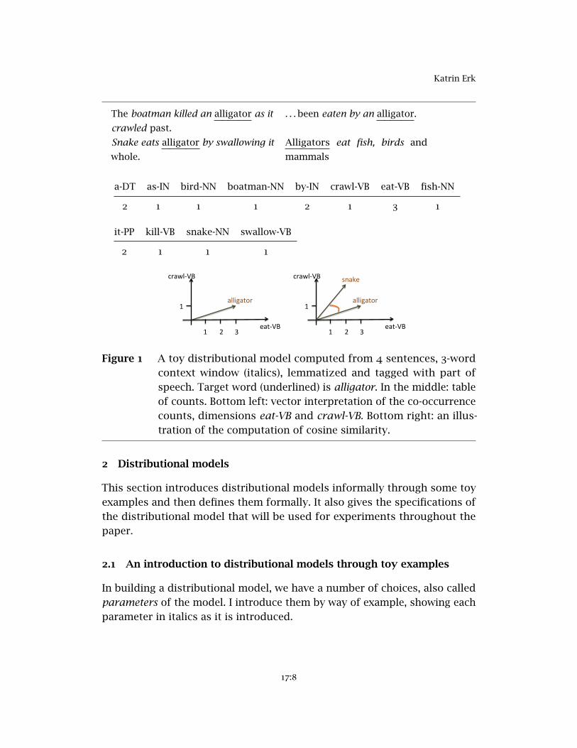
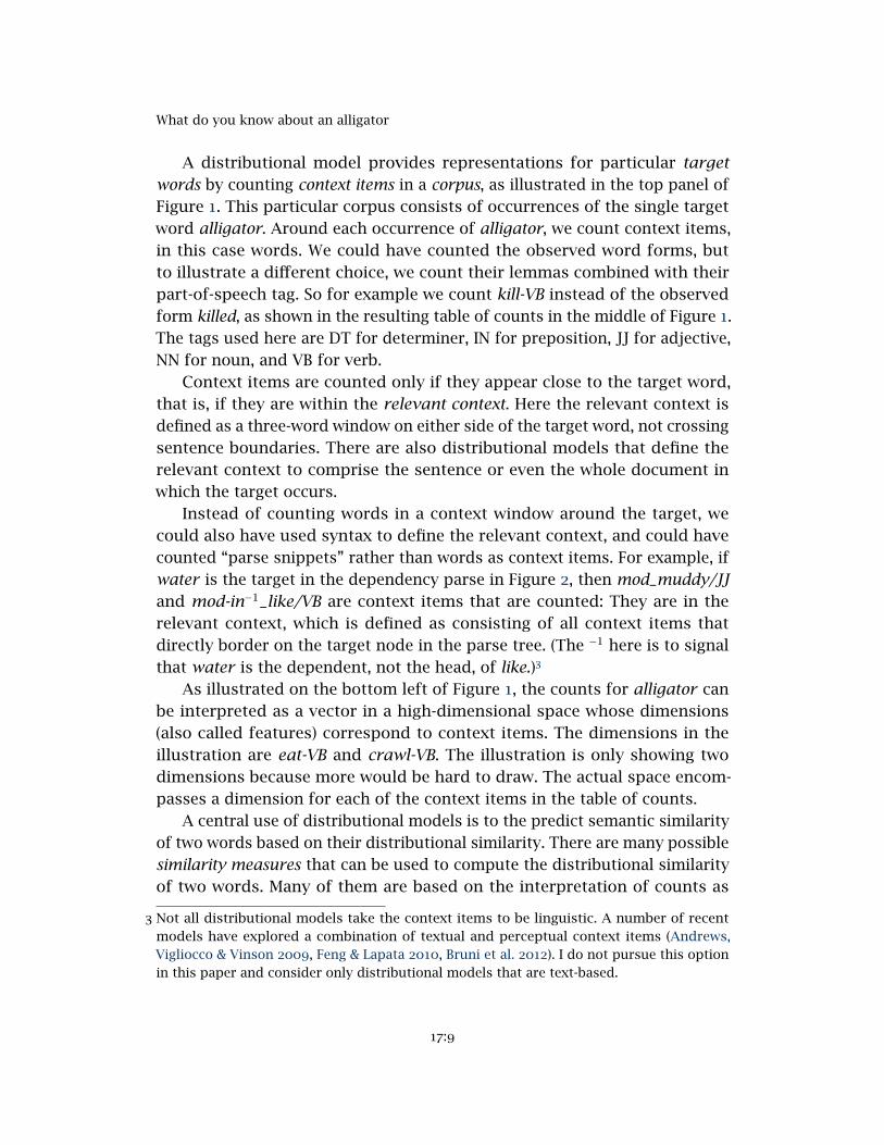
Figure 1 A toy distributional model computed from 4 sentences, 3-wordcontext window (italics), lemmatized and tagged with part ofspeech. Target word (underlined) is alligator. In the middle: tableof counts. Bottom left: vector interpretation of the co-occurrencecounts, dimensions eat-VB and crawl-VB. Bottom right: an illus-tration of the computation of cosine similarity.
2 Distributional models
This section introduces distributional models informally through some toyexamples and then defines them formally. It also gives the specifications ofthe distributional model that will be used for experiments throughout thepaper.
2.1 An introduction to distributional models through toy examples
In building a distributional model, we have a number of choices, also calledparameters of the model. I introduce them by way of example, showing eachparameter in italics as it is introduced.
17:8
What do you know about an alligator
A distributional model provides representations for particular targetwords by counting context items in a corpus, as illustrated in the top panel ofFigure 1. This particular corpus consists of occurrences of the single targetword alligator. Around each occurrence of alligator, we count context items,in this case words. We could have counted the observed word forms, butto illustrate a different choice, we count their lemmas combined with theirpart-of-speech tag. So for example we count kill-VB instead of the observedform killed, as shown in the resulting table of counts in the middle of Figure 1.The tags used here are DT for determiner, IN for preposition, JJ for adjective,NN for noun, and VB for verb.
Context items are counted only if they appear close to the target word,that is, if they are within the relevant context. Here the relevant context isdefined as a three-word window on either side of the target word, not crossingsentence boundaries. There are also distributional models that define therelevant context to comprise the sentence or even the whole document inwhich the target occurs.
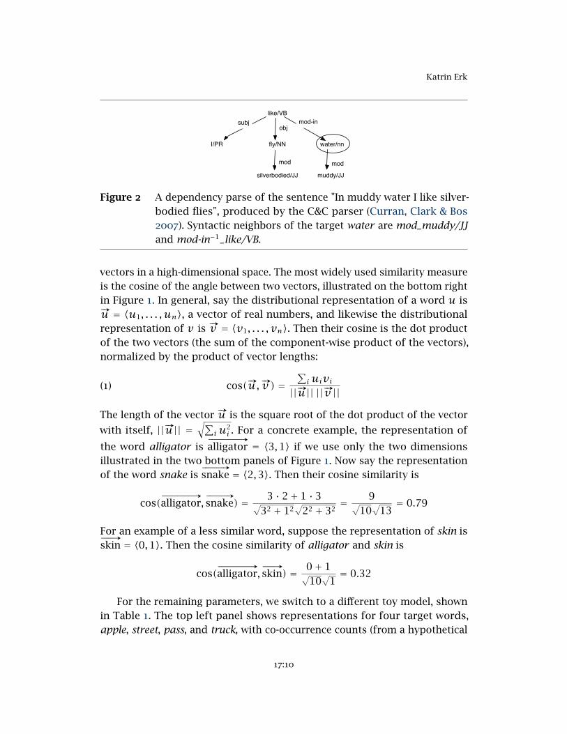
Instead of counting words in a context window around the target, wecould also have used syntax to define the relevant context, and could havecounted “parse snippets” rather than words as context items. For example, ifwater is the target in the dependency parse in Figure 2, then mod_muddy/JJand mod-in−1_like/VB are context items that are counted: They are in therelevant context, which is defined as consisting of all context items thatdirectly border on the target node in the parse tree. (The −1 here is to signalthat water is the dependent, not the head, of like.)3
As illustrated on the bottom left of Figure 1, the counts for alligator canbe interpreted as a vector in a high-dimensional space whose dimensions(also called features) correspond to context items. The dimensions in theillustration are eat-VB and crawl-VB. The illustration is only showing twodimensions because more would be hard to draw. The actual space encom-passes a dimension for each of the context items in the table of counts.
A central use of distributional models is to the predict semantic similarityof two words based on their distributional similarity. There are many possiblesimilarity measures that can be used to compute the distributional similarityof two words. Many of them are based on the interpretation of counts as
3 Not all distributional models take the context items to be linguistic. A number of recentmodels have explored a combination of textual and perceptual context items (Andrews,Vigliocco & Vinson 2009, Feng & Lapata 2010, Bruni et al. 2012). I do not pursue this optionin this paper and consider only distributional models that are text-based.
17:9
Katrin Erk
mod
like/VB
I/PR fly/NN water/nn
silverbodied/JJ muddy/JJ
mod-inobj
subj
mod
Figure 2 A dependency parse of the sentence "In muddy water I like silver-bodied flies", produced by the C&C parser (Curran, Clark & Bos2007). Syntactic neighbors of the target water are mod_muddy/JJand mod-in−1_like/VB.
vectors in a high-dimensional space. The most widely used similarity measureis the cosine of the angle between two vectors, illustrated on the bottom rightin Figure 1. In general, say the distributional representation of a word u is#»u = 〈u1, . . . , un〉, a vector of real numbers, and likewise the distributionalrepresentation of v is #»v = 〈v1, . . . , vn〉. Then their cosine is the dot productof the two vectors (the sum of the component-wise product of the vectors),normalized by the product of vector lengths:
(1) cos(#»u, #»v) =∑iuivi
|| #»u|| || #»v ||
The length of the vector #»u is the square root of the dot product of the vector
with itself, ||#»u|| =√∑
iu2i . For a concrete example, the representation of
the word alligator is# »
alligator = 〈3,1〉 if we use only the two dimensionsillustrated in the two bottom panels of Figure 1. Now say the representationof the word snake is
# »
snake = 〈2,3〉. Then their cosine similarity is
cos(# »
alligator,# »
snake) = 3 · 2+ 1 · 3√32 + 12
√22 + 32 =
9√10√13= 0.79
For an example of a less similar word, suppose the representation of skin is# »
skin = 〈0,1〉. Then the cosine similarity of alligator and skin is
cos(# »
alligator,# »
skin) = 0+ 1√10√1= 0.32
For the remaining parameters, we switch to a different toy model, shownin Table 1. The top left panel shows representations for four target words,apple, street, pass, and truck, with co-occurrence counts (from a hypothetical
17:10
What do you know about an alligator
crab car grass tree orange
apple 3 0 2 5 3
street 0 1 2 7 0
pass 2 5 1 0 5
truck 0 1 0 1 1
apple 0.59 0.0 0.18 0.14 0.0
street 0.0 0.0 0.44 0.74 0.0
pass 0.18 0.76 0.0 0.0 0.51
truck 0.0 0.62 0.0 0.0 0.37
d1 d2 d3
apple 0.11 0.36 0.51
street 0.03 0.83 -0.22
pass 0.93 -0.03 0.03
truck 0.71 -0.06 -0.11
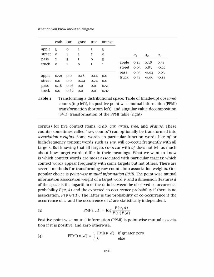
Table 1 Transforming a distributional space: Table of (made-up) observedcounts (top left), its positive point-wise mutual information (PPMI)transformation (bottom left), and singular value decomposition(SVD) transformation of the PPMI table (right)
corpus) for five context items, crab, car, grass, tree, and orange. Thesecounts (sometimes called “raw counts”) can optionally be transformed intoassociation weights. Some words, in particular function words like of orhigh-frequency content words such as say, will co-occur frequently with alltargets. But knowing that all targets co-occur with of does not tell us muchabout how target words differ in their meanings. What we want to knowis which context words are most associated with particular targets: whichcontext words appear frequently with some targets but not others. There areseveral methods for transforming raw counts into association weights. Onepopular choice is point-wise mutual information (PMI). The point-wise mutualinformation association weight of a target word v and a dimension (feature) dof the space is the logarithm of the ratio between the observed co-occurrenceprobability P(v,d) and the expected co-occurrence probability if there is noassociation, P(v)P(d). The latter is the probability of co-occurrence if theoccurrence of v and the occurrence of d are statistically independent.
(3) PMI(v,d) = logP(v,d)P(v)P(d)
Positive point-wise mutual information (PPMI) is point-wise mutual associa-tion if it is positive, and zero otherwise.
(4) PPMI(v,d) ={
PMI(v,d) if greater zero0 else
17:11
Katrin Erk
1 2 3 4
12
34
5
x
y
x'
y'
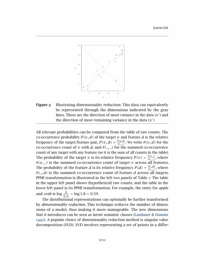
Figure 3 Illustrating dimensionality reduction: This data can equivalentlybe represented through the dimensions indicated by the graylines. These are the direction of most variance in the data (x′) andthe direction of most remaining variance in the data (y ′)
All relevant probabilities can be computed from the table of raw counts. Theco-occurrence probability P(v,d) of the target v and feature d is the relativefrequency of the target/feature pair, P(v,d) = #(v,d)
#(_,_) . We write #(v,d) for theco-occurrence count of v with d, and #(_, _) for the summed co-occurrencecount of any target with any feature (so it is the sum of all counts in the table).The probability of the target v is its relative frequency P(v) = #(v,_)
#(_,_) , where#(v, _) is the summed co-occurrence count of target v across all features.The probability of the feature d is its relative frequency P(d) = #(_,d)
#(_,_) , where#(_, d) is the summed co-occurrence count of feature d across all targets.PPMI transformation is illustrated in the left two panels of Table 1: The tablein the upper left panel shows (hypothetical) raw counts, and the table in thelower left panel is its PPMI transformation. For example, the entry for apple
and crab is log3391339
539= log1.8 = 0.59.
The distributional representations can optionally be further transformedby dimensionality reduction. This technique reduces the number of dimen-sions of a model, thus making it more manageable. The new dimensionsthat it introduces can be seen as latent semantic classes (Landauer & Dumais1997). A popular choice of dimensionality reduction method is singular valuedecomposition (SVD). SVD involves representing a set of points in a differ-
17:12
What do you know about an alligator
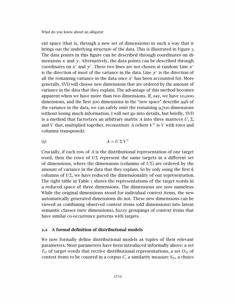
ent space (that is, through a new set of dimensions) in such a way that itbrings out the underlying structure of the data. This is illustrated in Figure 3.The data points in this figure can be described through coordinates on di-mensions x and y . Alternatively, the data points can be described throughcoordinates on x′ and y ′. These two lines are not chosen at random: Line x′
is the direction of most of the variance in the data. Line y ′ is the direction ofall the remaining variance in the data once x′ has been accounted for. Moregenerally, SVD will choose new dimensions that are ordered by the amount ofvariance in the data that they explain. The advantage of this method becomesapparent when we have more than two dimensions. If, say, we have 10,000dimensions, and the first 300 dimensions in the “new space” describe 99% ofthe variance in the data, we can safely omit the remaining 9,700 dimensionswithout losing much information. I will not go into details, but briefly, SVDis a method that factorizes an arbitrary matrix A into three matrices U , Σ,and V that, multiplied together, reconstitute A (where V T is V with rows andcolumns transposed):
(5) A = U Σ V T
Crucially, if each row of A is the distributional representation of one targetword, then the rows of UΣ represent the same targets in a different setof dimensions, where the dimensions (columns of UΣ) are ordered by theamount of variance in the data that they explain. So by only using the first kcolumns of UΣ, we have reduced the dimensionality of our representation.The right table in Table 1 shows the representations of the target words ina reduced space of three dimensions. The dimensions are now nameless:While the original dimensions stood for individual context items, the newautomatically generated dimensions do not. These new dimensions can beviewed as combining observed context items (old dimensions) into latentsemantic classes (new dimensions), fuzzy groupings of context items thathave similar co-occurrence patterns with targets.
2.2 A formal definition of distributional models
We now formally define distributional models as tuples of their relevantparameters. Most parameters have been introduced informally above: a setTD of target words that receive distributional representations, a set OD ofcontext items to be counted in a corpus C, a similarity measure SD, a choice
17:13
Katrin Erk
of relevant context in which to look for context items, and the options tocompute association weights and to do dimensionality reduction.TD and OD are arbitrary sets. We add a third set, the set of basis elements
BD that label the dimensions in the space that is eventually constructed.This can be the same as OD (as in the two tables on the left of Table 1), butif dimensionality reduction is used the basis elements will not be contextitems: In the right panel of Table 1 the basis elements are d1, d2, d3. Wedefine a corpus as a collection of targets and context items, C ∈ (OD ∪ TD)∗.The similarity function, which maps pairs of targets to a value indicatinga degree of distributional similarity, has the signature SD : (TD × TD) → R.We describe the relevant context as an extraction function XD that takes asinput the whole corpus C and returns co-occurrence counts of all targetswith all observable items from the set OD– that is, it returns a mapping fromtarget/context item pairs to numbers in N0 (as counts can also be zero). Insum, it has the signature XD : (TD ∪OD)∗ →
((TD ×OD)→ N0
). We lump the
optional association weight computation and dimensionality reduction stepsinto a single parameter, an aggregation function AD that takes the outputof XD and turns it into a mapping from targets and basis elements to realvalues, AD :
((TD ×OD)→ N0
)→((TD × BD)→ R
).
In summary, we describe distributional models as tuples comprising thesets of target elements, observable items, basis elements, the corpus, theextraction and aggregation function, and the similarity function:
(6) D = 〈TD,OD, BD,C, XD, AD, SD〉
The term “distributional” has been used for a number of different ap-proaches in computational linguistics. The definition above fits what Baroni,Dinu & Kruszewski (2014) call “count-based” models, which uses counts of co-occurring context items that are compiled into vectors in a high-dimensionalspace (Turney & Pantel 2010). A second class of approaches that is gettingincreasingly popular uses neural networks to compute word vectors (thencalled embeddings) based on some prediction task (Collobert & Weston 2008,Mikolov et al. 2010); some of these approaches will be covered by the defini-tion above, but maybe not all. Bayesian topic models (Blei, Ng & Jordan 2003)constitute a third class of distributional models. They are not covered by thedefinition above but could be covered by a slight variant.
17:14
What do you know about an alligator
2.3 The influence of parameters on distributional models
The choice of parameters has a large influence on the types of predictionsthat a distributional model will make. This is most obvious in the choiceof corpus C: Larger corpora are better in general as they yield more stableestimates of co-occurrence frequency. Another way in which the choice ofcorpus influences the model is through the genres that are represented in it.Lin (1998a), using a distributional model built from newspaper text, foundthat the words captive and westerner were respective nearest neighbors, thatis, westerner was the word most similar to captive among all the target words,and vice versa, a finding that clearly derives from kidnapping stories in thenewspapers. Note that such genre effects do not mean that the distributionalmodel is useless, just that it is noisy. Today most distributional approacheschoose to use the largest amount of corpus data possible to achieve the moststable estimates while diluting any genre effects.
As mentioned in the introduction, the extraction function XD is an impor-tant parameter that influences what a high similarity value means. Narrow-context models tend to give high ratings preferably to word pairs that areco-hyponyms (alligator/crocodile) or synonyms, while wide-context modelsalso give high ratings to pairs like alligator/swamp that stand in no tradi-tional semantic relation but are topically related. I discuss this parameter inmore depth in the following section.
Another parameter that influences what kinds of word pairs are givenhigh similarity ratings is the similarity function SD itself. Cosine tends to givehigh ratings to co-hyponym pairs, while other more recent measures aim togive high ratings to hyponym/hypernym pairs (Lenci & Benotto 2012, Roller,Erk & Boleda 2014, Fu et al. 2014).
In general, using association weights instead of raw counts leads to alarge improvement in performance. For dimensionality reduction the caseis not that clear. It sometimes leads to better performance, but not always.But a model with 300 dimensions is usually better manageable than one with10,000.
2.4 The distributional model used in this paper
All examples of distributional data in this paper use a common distributionalmodel. It is based on a corpus C that is a concatenation of the English Giga-word Corpus (news), the British National Corpus (mixed genres), a Wikipedia
17:15
Katrin Erk
dump called the English Wackypedia (encyclopedia text), and the ukWaCcorpus (web text) (Baroni, Bernardini, et al. 2009). The corpus was auto-matically lemmatized and tagged with parts of speech. Only nouns, propernouns, adjectives and verbs with a frequency of at least 500 were retained.The resulting corpus has roughly 2.8 billion tokens. As targets we use alllemma/tag pairs in this corpus; as context items we use the 20,000 mostfrequent lemma/tag pairs. Occurrences of context items are counted if theyare in a window of 2 words on either side of the target, not crossing sentenceboundaries.
The aggregation function AD in this model transforms counts to asso-ciation weights using PPMI (Equation (4)), and reduces the space to 500dimensions using SVD. We use cosine (Equation (1)) to compute distributionalsimilarity.4
3 Semantic relations: similarity versus relatedness
Having introduced distributional models and their parameters in general inthe previous section, I would now like to focus on one particular parameter,the extraction function XD. As mentioned above, distributional models haveoften been criticized (for example in G. L. Murphy 2002) for only yieldingvague “semantic similarity” ratings that do not provide evidence for anyparticular semantic relation. But two recent studies indicate that with somechoices of the extraction function XD, word pairs with high similarity ratingswill typically be related by a specific semantic relation, or a specific group ofrelations. This section discusses these studies in detail (so its aim is not tobreak new ground, but to report relevant results from the literature).
The question of whether distributional models can distinguish betweensemantic relations is critical for this paper because it is also a question ofinferences. If distributional models cannot distinguish between the relationsof alligator/crocodile and alligator/jaw, then it would be hard to see whatcould be inferred from alligator being similar to crocodile. But if it is possibleto build a distributional model in which pairs like alligator/crocodile are
4 When distributional models are used to model human language learning, any automaticprocessing like lemmatization or part-of-speech tagging is often avoided because thisinformation is not present in the input that humans receive. In this paper, I do not try tomodel infant language learning, where this is a clear concern. Instead, I model probabilisticinference by a competent speaker about individual unknown words. We can therefore assumethat the speaker is familiar with the lemmas and parts of speech of most of the contextitems observed to co-occur with the target words.
17:16
What do you know about an alligator
judged as similar, but pairs like alligator/jaw are not, then we can drawinferences about alligator from a high similarity rating to crocodile. (Whichinferences exactly we can get from a high similarity to crocodile is the subjectof Section 4.) Note that if distributional models can differ in this way, then theterm “similarity function” is actually somewhat misleading: It suggests thatall similarity functions approximate the same notion of similarity, while infact the function SD gives ratings that need to be interpreted differently basedon the definition of the function itself and based on the other parameters ofthe model, in particular the extraction function XD.
It will be helpful to have terminology that distinguishes between pairslike alligator/crocodile on the one hand and alligator/jaw on the other. Wetake over the distinction made by Peirsman 2008 and Agirre et al. 2009. Theyboth distinguish between similarity and relatedness. A pair of words is calledsimilar if they are synonyms, hypernym and hyponym, or co-hyponyms. Twowords are called related if they do not stand in a synonymy, hypernymy, orco-hyponymy relation but are still topically connected, such as alligator/jawor plane/pilot. I will use the terms AP-similarity and AP-relatedness to signalthese specific definitions of similarity and relatedness (“AP” for Agirre andPeirsman).
It has long been known anecdotally that the way to get high similarityratings for AP-similar words is to use a narrow context window of maybetwo or three words on either side of the target word, or a syntacticallydefined context as illustrated in Figure 2, see for example Sahlgren 2006.More recently, there have been two studies with empirical tests on the contextwindow effect: Peirsman 2008 for Dutch and Baroni & Lenci 2011 for English.
In the introduction I have already briefly discussed the question of whythe choice of context window can have such an effect: It is because with anarrow context window, the context items found for a noun target will oftenbe modifiers, or verbs that take the target as an argument. In either case, thecontext items indicate selectional constraints that the noun target meets –and such constraints are typically expressed in terms of properties. If twonoun targets agree in many of the modifiers or verbs that they appear with,then they will typically share many semantic properties, like synonyms orco-hyponyms do. In a wide context window, the context items will be muchmore mixed.
Back to the two empirical studies of the context window effect. Peirsman(2008) tests several distributional models trained on Dutch newspaper text,using cosine to compute similarity and varying the context window between
17:17
Katrin Erk
concept concept class relation relatum
alligator-n amphibian_reptile cohypo toad-n
alligator-n amphibian_reptile hyper carnivore-n
alligator-n amphibian_reptile mero jaw-n
alligator-n amphibian_reptile attri frightening-j
alligator-n amphibian_reptile event bask-v
alligator-n amphibian_reptile random-j constructive-j
alligator-n amphibian_reptile random-n trombone-n
alligator-n amphibian_reptile random-v fetch-v
Table 2 Sample entries from the BLESS dataset
1 and 20 words (ignoring sentence boundaries). He also tests a distributionalmodel where context is defined as syntactic neighborhood (as in Figure 2),and similarity is again computed using cosine. Peirsman tests how many ofthe target nouns are synonyms, co-hyponyms, or direct hypo- or hypernymsof their single nearest distributional neighbor (that is, the noun that has thehighest similarity rating to the target). Peirsman finds that the proportionof nearest neighbors that are AP-similar is largest for the syntactic-contextdistributional model, and that for the context-window models it generallydecreases with window size. This study allows for a tentative conclusionthat models with a syntactic definition of context or with a narrow contextwindow have a tendency to give high similarity ratings to AP-similar words.The study also finds that across distributional models, the largest percentageof AP-similar nearest neighbors tend to be co-hyponyms.
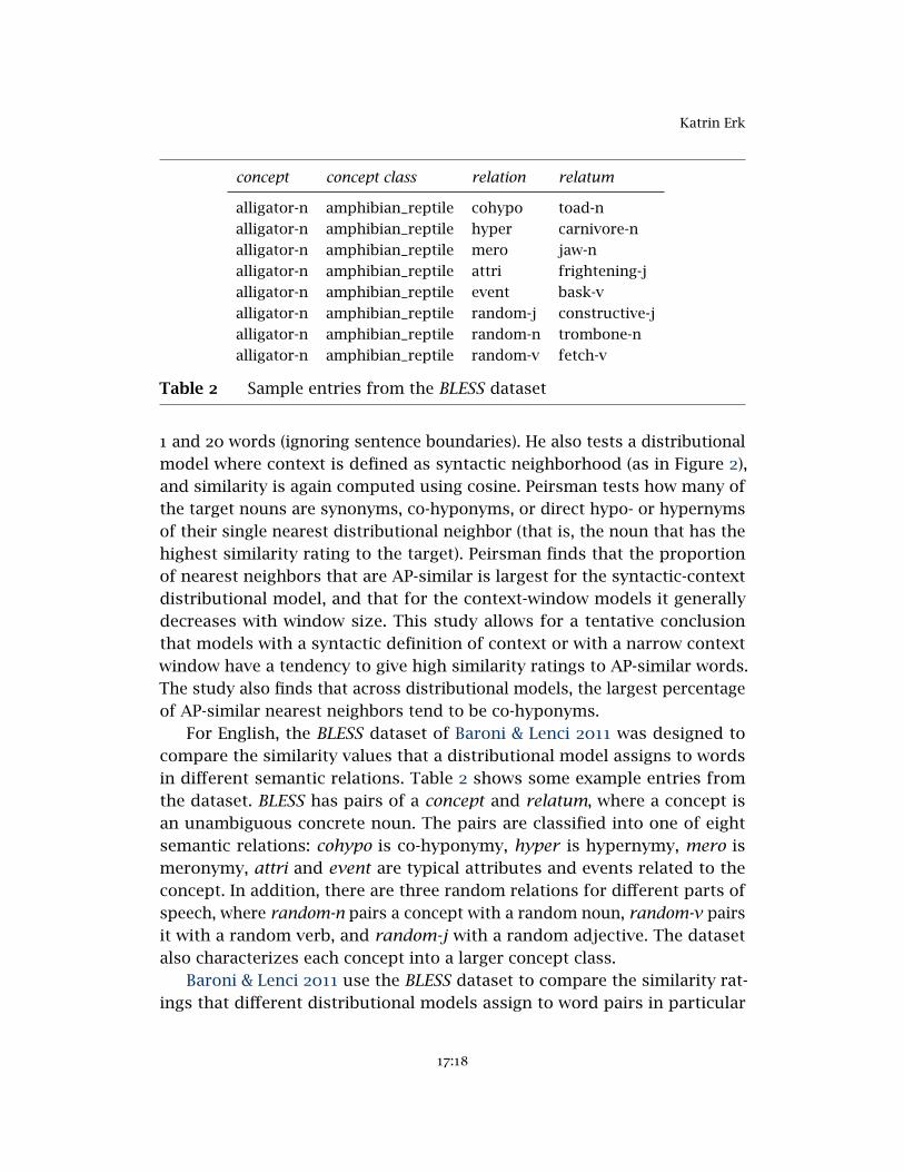
For English, the BLESS dataset of Baroni & Lenci 2011 was designed tocompare the similarity values that a distributional model assigns to wordsin different semantic relations. Table 2 shows some example entries fromthe dataset. BLESS has pairs of a concept and relatum, where a concept isan unambiguous concrete noun. The pairs are classified into one of eightsemantic relations: cohypo is co-hyponymy, hyper is hypernymy, mero ismeronymy, attri and event are typical attributes and events related to theconcept. In addition, there are three random relations for different parts ofspeech, where random-n pairs a concept with a random noun, random-v pairsit with a random verb, and random-j with a random adjective. The datasetalso characterizes each concept into a larger concept class.
Baroni & Lenci 2011 use the BLESS dataset to compare the similarity rat-ings that different distributional models assign to word pairs in particular
17:18
What do you know about an alligator
semantic relations. They evaluate distributional models in which all parame-ters are kept fixed except for the context size: two models that use contextwindows, one narrow (2 content words on either side of the target word)and one wide (20 content words either side), and a model that considersthe whole document as the context for an occurrence of the target word.The similarity measure in these experiments is again cosine. To evaluatethe models, they determine the similarity of each target to its nearest (mostsimilar) relatum in each of the 8 relations. They then compare the collectedsimilarities for co-hyponyms, hypernyms, meronyms, and so on. In all threedistributional models, co-hyponyms have the highest similarity to the targets.But in the document-based model, the difference of co-hyponyms particularlyto hypernyms, meronyms, and events is very slight. It is more marked inthe 20-word context window model, and quite strong in the 2-word contextwindow model. That is, a document-based model captures a wide varietyof relations with similar strength, while a narrow context window makesco-hyponymy prominent. I repeated the experiment with a distributionalmodel with syntax-based context and found that, as expected, models with asyntactic context show similar results to narrow context window models.
4 Property Overlap
In both experiments reported in the previous section, Peirsman 2008 andBaroni & Lenci 2011, narrow context window and syntactic context windowmodels tend to give the highest similarity ratings to AP-similar word pairs,in particular co-hyponyms. In this section we ask which inferences an agentcan draw from observing that two words are highly AP-similar. This wouldbe easy if all AP-similar word pairs were in a single semantic relation, butAP-similarity encompasses synonymy, hypernymy, and co-hyponymy.
One could argue that as distributional models tend to give the highestAP-similarity ratings to co-hyponym pairs, we should take AP-similarity sim-ply as an indication of co-hyponymy and ignore the other relations. Butco-hyponymy is not well-defined. Because it is the relation between sisterterms in a taxonomy, it depends strongly on details of the taxonomy. InBLESS, where the relevant higher-level concept class for alligator is amphib-ian_reptile, its co-hyponyms are crocodile, frog, lizard, snake, toad and turtle.In WordNet (Fellbaum 1998), a more fine-grained taxonomy, the direct hy-pernym of alligator is crocodilian. There crocodile is still a sister term ofalligator, but frog and the others are not.
17:19
Katrin Erk
Instead I am going to argue that AP-similarity can be characterized asproperty overlap, where “property” is again meant in a broad sense that en-compasses hypernyms and in fact any predicates that apply to all membersof a category. Co-hyponyms have many properties in common. This includestheir joint hypernyms: Alligators and crocodiles are both reptiles, and theyare both animals. They also share other properties: Alligators and crocodilesare both green, both dangerous, and both scaly. Property overlap also accom-modates relations other than co-hyponymy that are included in AP-similarity:Synonyms share most of their properties, and likewise hypernym-hyponympairs. On the other hand, words that are only AP-related, like alligator/swamp,do not usually share many properties. Interpreting AP-similarity as propertyoverlap allows us to draw inferences from observed distributional similarity:If alligator and crocodile are distributionally highly similar, we infer that theymust have many properties in common.
But before we conclude that AP-similarity is property overlap, we need toconsider some possible counter-arguments. First, given that co-hyponymsgenerally receive the highest similarity ratings from distributional modelsof AP-similarity, we need to ask if property overlap is the best possiblecharacterization of co-hyponymy. Typical examples of co-hyponymy arealligator and crocodile, or cat and dog. These pairs share many properties– but they are also incompatible, that is, there is no entity that is both analligator and a crocodile, or both a cat and a dog. If all co-hyponym pairs wereincompatible, then we might have to characterize AP-similarity as somethinglike property overlap plus incompatibility. But as Cruse (2000) points out(Section 9.1), many co-hyponyms in existing taxonomies are not incompatible.If we look at the direct hyponyms of the word man (in the sense of adultmale) in WordNet, we find terms like bachelor, boyfriend, dandy and father-figure, which are certainly compatible. In BLESS, the larger category buildingcontains castle, hospital, hotel, restaurant, villa. Some of these words areprobably incompatible, but not all. So as co-hyponymy does not entail eithercompatibility or incompatibility, we can leave compatibility out of the picturewhen interpreting AP-similarity.
Another possible counter-argument to interpreting AP-similarity as prop-erty overlap is that relatively few hypernym-hyponym pairs get high AP-similarity ratings, even though hyponyms and hypernyms overlap in all theproperties of the hypernym. To see why few hypernym-hyponym pairs gethigh AP-similarity ratings, it is useful again to look at what distributionalmodels do. Distributional similarity is high if two target words occur in many
17:20
What do you know about an alligator
of the same contexts, which, as I have argued above, is the case if they sharemany properties – but this is not the only factor that determines whethertwo words will occur in the same contexts. Similar level of generality andsimilar register are two other relevant factors. The words dog and mammalwill rarely occur in the same contexts because mammal is a much moreformal term than dog, as well as a much more general concept. What followsfrom that is that we should take high distributional similarity as a sign ofhigh property overlap, but we should not take low distributional similarity asa sign of low property overlap. Rather, low distributional similarity shouldjust be read as a sign that there is too little information to judge propertyoverlap. The model that I formulate in Section 6 will do exactly that: It willdraw inferences from high degrees of distributional similarity, but not fromlow distributional similarity.
Existing work on inferring properties from distributional data. There issome empirical evidence that distributional data can be used for inferringproperties in Johns & Jones 2012, Fagarasan, Vecchi & Clark 2015, Guptaet al. 2015, and Herbelot & Vecchi 2015. They test whether distributionalvectors can be used to predict a word’s properties (where, as above, I usethe term “properties of a word” to mean properties that apply to all entitiesin the word’s extension). To do so, they either make use of distributionalsimilarity directly, or use regression to learn a mapping from distributionalvectors to “property vectors”. All except Gupta et al. use as data the featurenorms in McRae et al. 2005 and in Vigliocco et al. 2004. This is data collectedthrough experiments in which participants were asked to provide definitionalfeatures for particular words. I take these papers as preliminary evidencethat distributional data can indeed be used as a basis for property inference.However, I cannot use any of these approaches directly in this paper; somecompute (uninterpretable) weights rather than probabilities, some have adifferent task from the one I am addressing.5
There are also several recent papers that focus specifically on the pre-diction of hypernyms from distributional data (Lenci & Benotto 2012, Roller,
5 The most similar approach to mine is the one of Herbelot and Vecchi. They have a set-theoretic motivation for the property vectors they use. The numbers in their property vectorsencode whether “all”, “most”, “some”, or “few” members of a category have a particularproperty, where each quantifier is represented by a fixed probability. But the approach doesnot fit into the setting I use because it is unclear how these probability vectors could beintegrated into possible worlds.
17:21
Katrin Erk
Erk & Boleda 2014, Fu et al. 2014), though there is some debate on the extentto which particular methods allow for hypernymy inference (O. Levy et al.2015). And work on mapping distributional representations to low-level visualfeatures (Lazaridou, Bruni & Baroni 2014) is also relevant if we consider thosevisual features as cues towards visual properties such as colors.
Properties of words can also be induced more directly from distributionaldata, for example from the sentence He saw the dangerous alligator one canlearn that alligators are sometimes dangerous (Almuhareb & Poesio 2004,2005, Devereux et al. 2009, Kremer & Baroni 2010, Baroni, B. Murphy, et al.2010, Baroni & Lenci 2010). It is difficult, with this technique, to learn the kindsof properties that humans give in feature norm experiments. Devereux et al.(2009) conclude that high-accuracy extraction of properties is unrealistic atthis point in time. But it may be that extraction of exactly the same propertiesthat humans tend to list is not what these models are good at. Baroni, B.Murphy, et al. (2010) observe the “tendency of [their model], when comparedwith the human judgments in the norms, to prefer actional and situationalproperties (riding, parking, colliding, being on the road) over parts (suchas wheels and engines)” (p. 233). Thill, Pado & Ziemke (2014) suggest thatthe distributional features in models like the one of Baroni & Lenci (2010),which list closely co-occurring words, can reveal the “human experience ofconcepts.” So it is possible that (some) distributional features themselvesshould also be considered as properties. This is an issue that I will not pursuefurther in the current paper, but that should be taken up again later.
5 A probabilistic information state
As discussed in the introduction, the two main aims of this paper are first, toargue that distributional inference (by the right kind of model) is propertyinference, and second, to propose a probabilistic inference mechanism for in-tegrating distributional evidence with formal semantics. Section 4 addressedthe first aim. Section 6 will address the second aim. This section lays thegroundwork for Section 6 by defining probabilistic information states. If anagent is completely sure that crocodiles are animals, we will express this byhaving the probabilistic information state assign a probability of 1 to thestatement crocodiles are animals. If the agent is unsure whether it is truethat alligators are animals, their probabilistic information state will assign aprobability of less than 1 to this statement (but greater than 0, because thatwould mean that the agent is sure that alligators are not animals).
17:22
What do you know about an alligator
5.1 Probabilistic semantics
I will give a probabilistic account of an agent’s information state in termsof probabilistic logic (Nilsson 1986), which has a probability distributionover worlds to indicate uncertainty about the nature of the actual world.Probabilistic logic is easy to formulate in the case of finitely many worlds,but even though Clarke & Keller (2015) formulate it for the infinite case, itis not clear at this point how updates to the probability distribution extendto the infinite case. I argue below in Section 5.3 why I use probabilistic logicanyway. For now I use a definition that only allows for finitely many worlds.
As a basis for probabilistic logic, we use standard first-order logic lan-guages L with the following syntax. Let IC be a set of individual constants,and IV a set of individual variables. Then the set of terms is defined asIC ∪ IV . Let PSn be a collection of n-place predicate symbols for n ≥ 0. Theset of formulas is defined inductively as follows. If R is an n-ary predicatesymbols and t1, . . . , tn are terms, then R(t1, . . . , tn) is a formula. If φ1, φ2 areformulas, then so are ¬φ1 and φ1 ∧φ2 and φ1 ∨φ2. If x is a variable and φis a formula, then so are ∀xφ and ∃xφ. A sentence of L is a formula withoutfree variables. A probabilistic model for L is a structure M = 〈U,W ,V ,P〉where U is a nonempty universe,W is a nonempty and finite set of worlds,6
and V is a valuation function that assigns values as follows. It assigns in-dividuals from U to individual constants from IC. To an n-place predicatesymbol u ∈ PSn it assigns a functionW →Un. V (u)(w) is the extension ofu in the worldw . P is a probability distribution overW . Then the probabilityof a sentence ϕ of L is the summed probability of all worlds that make ittrue:
(7) P(ϕ) =∑w∈W
{P(w) | �ϕ�w = T}
5.2 A probabilistic information state
We use probabilistic logic for describing the information state of an agent.Information states have been used in update semantics (Veltman 1996), wherean information state is a set of worlds that, as far as the agent knows, could
6 Systems that work with probabilistic logic in practice, such as Markov Logic Net-works (Richardson & Domingos 2006), usually assume a finite domainU that is in one-to-onecorrespondence with a finite set IC of constants, and a finite set of predicate symbols. Butminimally, what is needed is that the set of worldsW be finite.
17:23
Katrin Erk
be the actual world. In a probabilistic information state, the agent considerssome worlds more likely than others to be the actual world (van Benthem,Gerbrandy & Kooi 2009, van Eijck & Lappin 2012, Zeevat 2013).
We define a probabilistic information state over language L to be a prob-abilistic modelM for L. While update semantics focuses on the way that asingle sentence updates the information state, we are interested in describinghow the probability distribution over worlds is affected by distributionalinformation when that distributional information contains clues about themeaning of a word u. After all, the probability that an agent ascribes to aworld depends, among other things, on the agent’s belief about what wordsmean.
For example, assume that the distributional similarity of crocodile andalligator is 0.93. We will call this a piece of distributional evidence Edist. 0.93is a high similarity rating, so we would be likely to see this evidence if theactual world is a world w1 in which entities that are alligators and entitiesthat are crocodiles have many properties in common. We would not be solikely to see this evidence if the actual world was a world w2 where alligatorsand crocodiles do not have many properties in common. In our case, theagent should assign a higher probability to w1 and assign a lower probabilityto w2 on the basis of Edist. This can be described through Bayesian beliefupdate, which in this case would use the probability of the distributionalevidence in a world to compute the inverse: the probability of a world giventhe distributional evidence. Bayesian update transforms a prior belief, in ourcase a prior probability distribution P0 over worlds, into a posterior belief,in our case a probability distribution P1 that describes the probability ofeach world w after the distributional evidence has been seen. It does so byweighting the prior probability of w against the probability of the evidencein world w, and normalizing by the probability of the evidence.
(8) P1(w) = P(w|Edist) =P(Edist|w)P0(w)
P(Edist)
The probability of the evidence P(Edist) in the denominator of (8) is computedas the sum of the probability of Edist under all worlds w′ weighted by theprobabilities of those worlds:
(9) P(Edist) =∑w′P(Edist|w′)P0(w′)
Equation (8) contains three different probabilities: the prior P0, which wetake to be given, the posterior P1, which we compute, and the probability
17:24
What do you know about an alligator
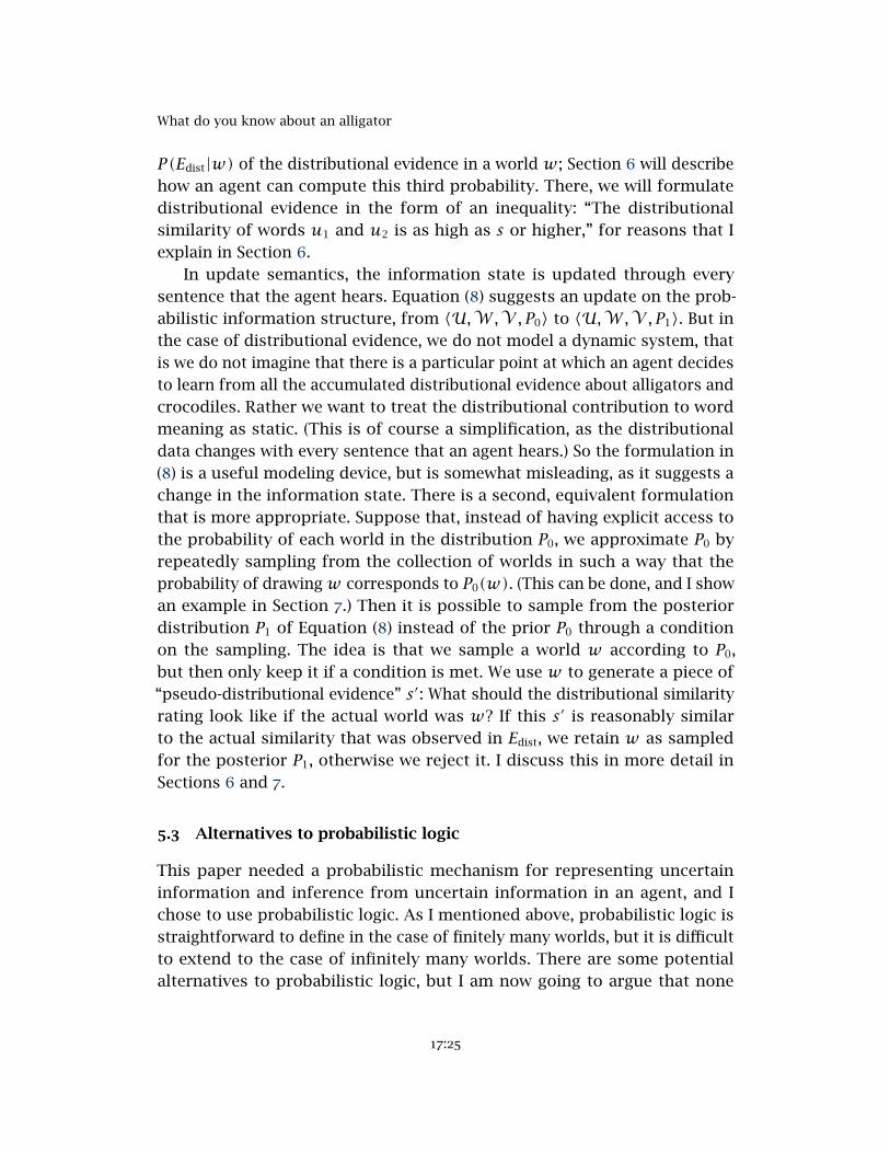
P(Edist|w) of the distributional evidence in a world w ; Section 6 will describehow an agent can compute this third probability. There, we will formulatedistributional evidence in the form of an inequality: “The distributionalsimilarity of words u1 and u2 is as high as s or higher,” for reasons that Iexplain in Section 6.
In update semantics, the information state is updated through everysentence that the agent hears. Equation (8) suggests an update on the prob-abilistic information structure, from 〈U,W ,V , P0〉 to 〈U,W ,V , P1〉. But inthe case of distributional evidence, we do not model a dynamic system, thatis we do not imagine that there is a particular point at which an agent decidesto learn from all the accumulated distributional evidence about alligators andcrocodiles. Rather we want to treat the distributional contribution to wordmeaning as static. (This is of course a simplification, as the distributionaldata changes with every sentence that an agent hears.) So the formulation in(8) is a useful modeling device, but is somewhat misleading, as it suggests achange in the information state. There is a second, equivalent formulationthat is more appropriate. Suppose that, instead of having explicit access tothe probability of each world in the distribution P0, we approximate P0 byrepeatedly sampling from the collection of worlds in such a way that theprobability of drawingw corresponds to P0(w). (This can be done, and I showan example in Section 7.) Then it is possible to sample from the posteriordistribution P1 of Equation (8) instead of the prior P0 through a conditionon the sampling. The idea is that we sample a world w according to P0,but then only keep it if a condition is met. We use w to generate a piece of“pseudo-distributional evidence” s′: What should the distributional similarityrating look like if the actual world was w? If this s′ is reasonably similarto the actual similarity that was observed in Edist, we retain w as sampledfor the posterior P1, otherwise we reject it. I discuss this in more detail inSections 6 and 7.
5.3 Alternatives to probabilistic logic
This paper needed a probabilistic mechanism for representing uncertaininformation and inference from uncertain information in an agent, and Ichose to use probabilistic logic. As I mentioned above, probabilistic logic isstraightforward to define in the case of finitely many worlds, but it is difficultto extend to the case of infinitely many worlds. There are some potentialalternatives to probabilistic logic, but I am now going to argue that none
17:25
Katrin Erk
of them is currently viable for my purposes. So like Zeevat (2013), I chooseto use probabilistic logic in spite of its problems because it allows us toexplore the connection of probabilities and logic in a framework that is closeto standard model-theoretic semantics.
Fuzzy logic (Zadeh 1965) is a many-valued logic in which formulas areassigned values between 0 and 1 that indicate their degrees of truth, andit can represent uncertainty in that way. Fuzzy logic is a truth-functionalapproach, as the truth value of a complex formula is a function of the truthvalues of its components. For example, the truth value of a formula F ∧G isthe minimum of the values of F and G. The problem with truth-functionalapproaches is that they miss penumbral connections (Fine 1975, van Deemter2013), like the fact that an object cannot be all pink and all red at the sametime. If an object b is on the borderline of pink and red, the weights for“b is pink” and “b is red” could both be 0.5. In that case the value for “b ispink and b is red” will be 0.5 as well, while it should be zero (false). Becauseit produces counter-intuitive truth degrees of this kind, I would rather usemore principled alternatives to fuzzy logic.
Cooper et al. (2014) focus on the interaction between perception andsemantic interpretation. They use a type-theoretic setting, in which situationsare judged as being of particular types, which can be arbitrary propositions(among other things). Probabilities are associated with these judgments. Theprobabilities are assumed to come from a classifier that takes as input eithersome feature-based perceptual representation of a situation or a collectionof previous types assigned to the same situation, and classifies it as beingof a particular type with a certain probability. So penumbral connectionswill be taken into consideration only to the extent that the classifier haslearned to respect them. That is, if the classifier never sees a situation inwhich something is completely pink and completely red at the same time,the probability of “b is pink and b is red” will be zero – but this informationcan only be learned by the classifier, and the classifier is a black box. Nodeclarative knowledge can be injected into it. So I do not use the framework ofCooper et al. because it would constrain me to knowledge collected by directperception, while I want to study the interaction of declarative knowledgewith information coming from distributional evidence.
Goodman, Tenenbaum & Gerstenberg (to appear) and Goodman & Lassiter(2014) propose that in understanding an utterance the hearer builds a mentalsituation. So their approach is situation-based like the one of Cooper et al.,but their situations are imagined, while Cooper et al. use perception of real
17:26
What do you know about an alligator
situations. The hearer generates a mental situation based on probabilisticknowledge (where Goodman et al. do not make a distinction between generalworld knowledge and linguistic knowledge) encoded in probabilistic genera-tive statements like: “To generate a person, draw their gender by flipping afair coin, then draw their height from the normal distribution of heights forthat gender.” I do not use their approach because it focuses on generatingmental situations based on individual utterances, and the current paper isnot about updating the information state based on individual utterances.But generative models are widely used in machine learning (Bishop 2006),and the idea of using a generative approach to assemble a situation or worldprobabilistically (which is introduced in more detail below) is general enoughthat it can be used to implement the model introduced in this paper. It isjust that in our case what is generated is not a situation but a world. Good-man, Mansighka, et al. (2008) have developed a programming language forspecifying (small) probabilistic generative models, which is general-purposeand not restricted to implementing the specific model of Goodman et al. Iuse it for a proof of concept experiment in Section 7.
6 Probabilistically inferring properties from distributional evidence
This section introduces a mechanism by which distributional inference caninfluence the probabilistic information state. In the previous section I havedescribed the effect of distributional evidence as a (Bayesian) update on aprobability distribution over worlds, with a formula that is repeated herefor convenience: The prior belief P0(w), or probability that the agent assignsto w being the actual world, is transformed into a posterior belief P1(w) =P(w|Edist) after seeing the distributional evidence Edist, which is about adistributional similarity rating for a particular pair of words:
(8) P1(w) = P(w|Edist) =P(Edist|w)P0(w)
P(Edist)
The Bayesian update in Equation (8) has three components: the prior prob-ability P0(w) of the world w, the posterior probability P1(w) of w afterseeing the evidence Edist, and the probability of the distributional evidence inthe world w, P(Edist|w). (The denominator, P(Edist), can be factored into thesame components, as shown in the previous section.) The prior is given. Toobtain the posterior, we need to compute P(Edist|w). This section shows howthat can be done.
17:27
Katrin Erk
6.1 The story in a nutshell
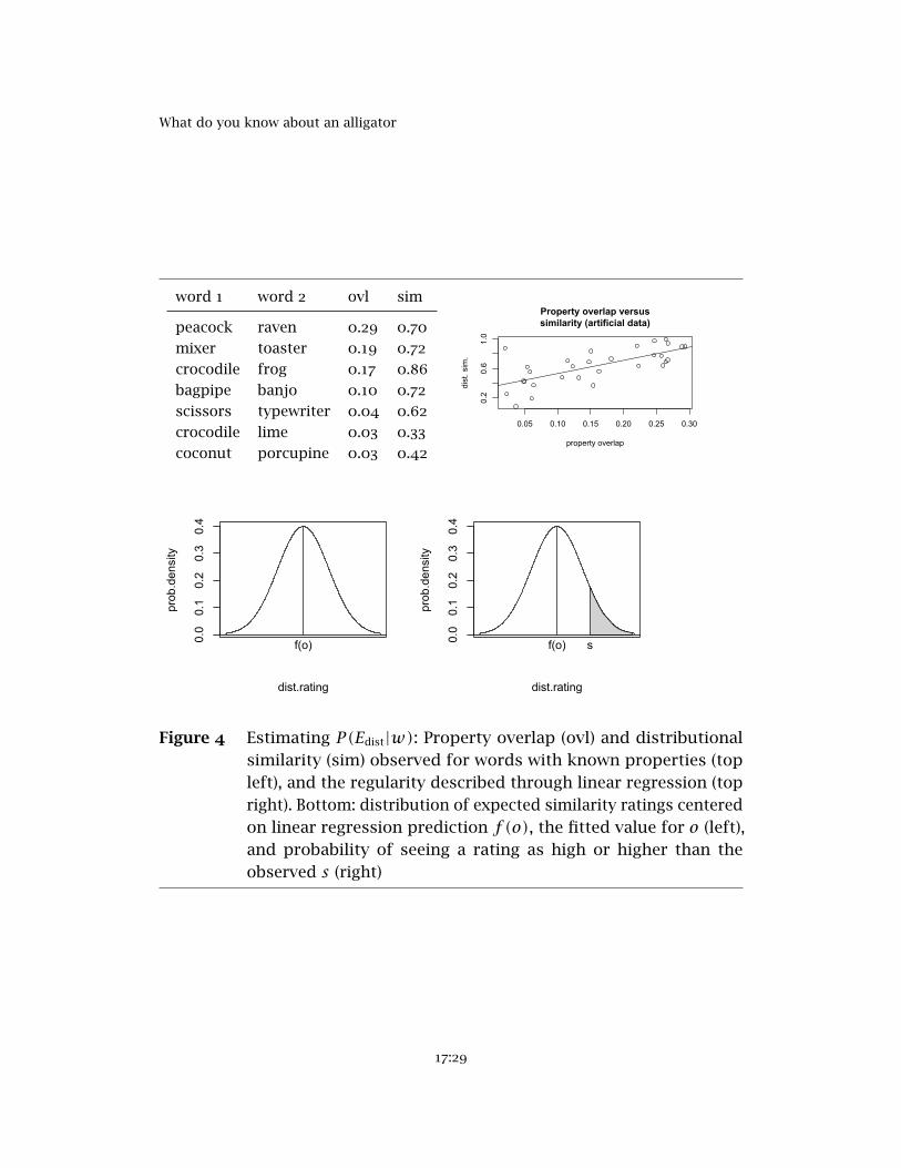
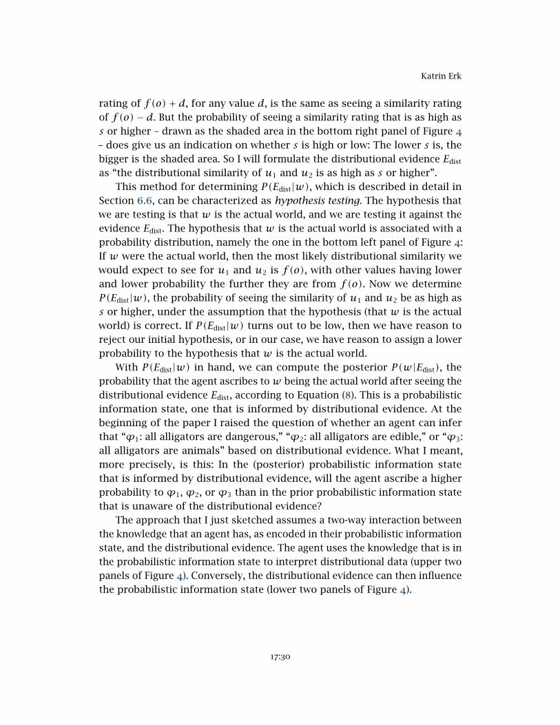
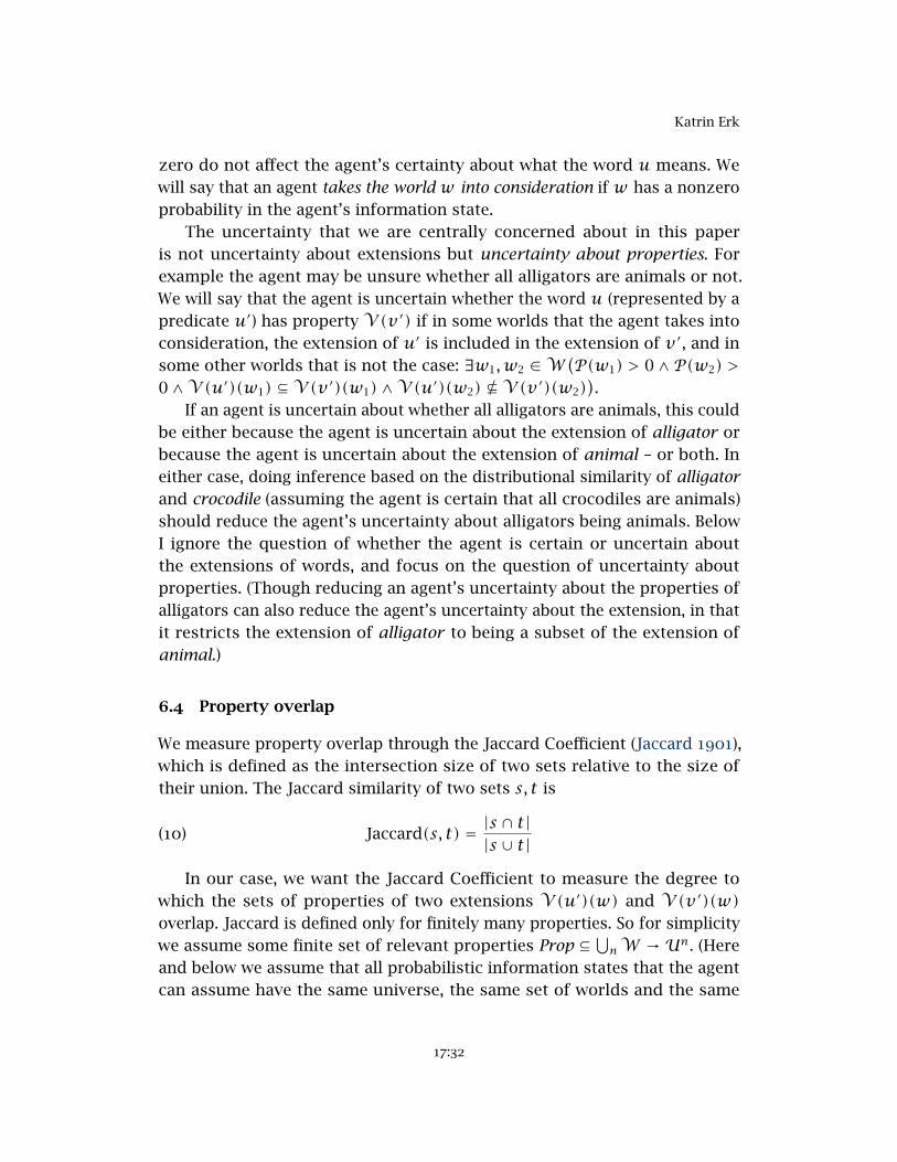
Before I go into the details of the model, I first give an overview of its pieces.Each distributional similarity value is a weight, and to use it as evidence, theagent first needs to interpret it: What kinds of distributional similarity valuestypically occur when property overlap is high? And for low property overlap?The top left panel of Table 4 gives an example. It shows pairs of words forwhich we assume the agent knows the property overlap (“ovl”), along with thedistributional similarity (“sim”) that the agent observes for them. (Section 6.4below defines what I mean by “knowing the property overlap.”) What theagent can observe in this case is that high property overlap tends to go withhigh distributional similarity, and vice versa. This observation can in thesimplest case be described as a linear relation, as sketched in the top rightpanel of Table 4.
When the agent has inferred this linear relationship, they can take aproperty overlap o between the extensions of two words u1 and u2 andpredict what the distributional similarity f(o) of u1 and u2 should be,simply by reading off the appropriate y-value (similarity) for the given x-value(overlap). Here, f(.) is a function that maps an overlap value o to its fittedvalue, the model’s prediction for o. And the agent can go one step further:The data is somewhat noisy, in that the distributional similarity is usuallynot exactly equal to the value f(o). But it will most likely be close to f(o),and will be less likely to be much higher or much lower than that. This can bedescribed as a probability distribution over possible similarity values givenoverlap o. It has its mean at f(o), as sketched in the bottom left panel ofFigure 4. Section 6.5 describes this probability distribution in more detail.
This probability distribution can then be used to estimate P(Edist|w),the probability that this section is about: Suppose the property overlap ofthe extensions of u1 and u2 in world w is o, the distributional similaritythat the agent predicts from overlap o is f(o), and the actually measureddistributional similarity of u1 and u2 is s. What is the probability of thisdistributional evidence given w , which is to say, given that the property over-lap is o? This can be read off the probability distribution in the bottom leftpanel of Figure 4, which is a probability distribution over the distributionalsimilarity values we expect to see given that the overlap is o. But what weneed is not the probability of seeing a similarity rating of exactly s. Thisprobability does not say anything about whether s is high or low, as the prob-ability distribution is symmetric, and the probability of seeing a similarity
17:28
What do you know about an alligator
word 1 word 2 ovl sim
peacock raven 0.29 0.70
mixer toaster 0.19 0.72
crocodile frog 0.17 0.86
bagpipe banjo 0.10 0.72
scissors typewriter 0.04 0.62
crocodile lime 0.03 0.33
coconut porcupine 0.03 0.42
0.05 0.10 0.15 0.20 0.25 0.30
0.2
0.6
1.0
Property overlap versussimilarity (artificial data)
property overlap
dist
. sim
.
0.00.10.20.30.4
dist.rating
prob.density
f(o) 0.00.10.20.30.4
dist.rating
prob.density
f(o) s
Figure 4 Estimating P(Edist|w): Property overlap (ovl) and distributionalsimilarity (sim) observed for words with known properties (topleft), and the regularity described through linear regression (topright). Bottom: distribution of expected similarity ratings centeredon linear regression prediction f(o), the fitted value for o (left),and probability of seeing a rating as high or higher than theobserved s (right)
17:29
Katrin Erk
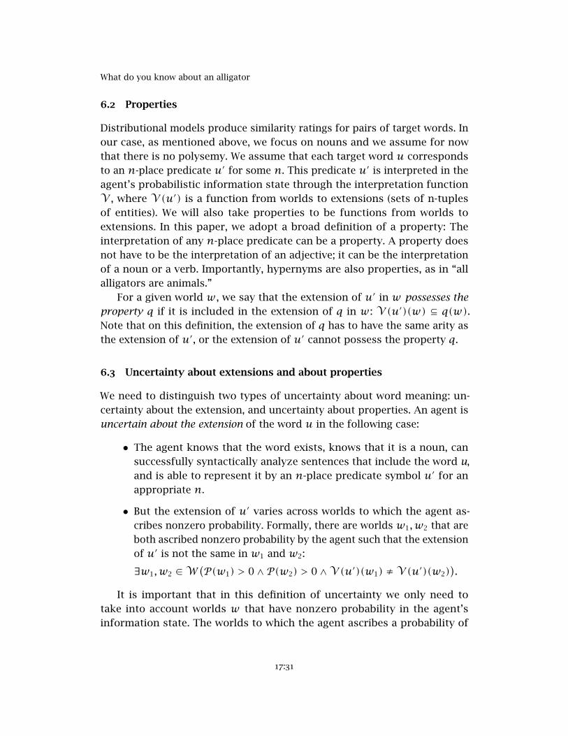
rating of f(o)+ d, for any value d, is the same as seeing a similarity ratingof f(o)− d. But the probability of seeing a similarity rating that is as high ass or higher – drawn as the shaded area in the bottom right panel of Figure 4– does give us an indication on whether s is high or low: The lower s is, thebigger is the shaded area. So I will formulate the distributional evidence Edist
as “the distributional similarity of u1 and u2 is as high as s or higher”.This method for determining P(Edist|w), which is described in detail in
Section 6.6, can be characterized as hypothesis testing. The hypothesis thatwe are testing is that w is the actual world, and we are testing it against theevidence Edist. The hypothesis that w is the actual world is associated with aprobability distribution, namely the one in the bottom left panel of Figure 4:If w were the actual world, then the most likely distributional similarity wewould expect to see for u1 and u2 is f(o), with other values having lowerand lower probability the further they are from f(o). Now we determineP(Edist|w), the probability of seeing the similarity of u1 and u2 be as high ass or higher, under the assumption that the hypothesis (that w is the actualworld) is correct. If P(Edist|w) turns out to be low, then we have reason toreject our initial hypothesis, or in our case, we have reason to assign a lowerprobability to the hypothesis that w is the actual world.
With P(Edist|w) in hand, we can compute the posterior P(w|Edist), theprobability that the agent ascribes tow being the actual world after seeing thedistributional evidence Edist, according to Equation (8). This is a probabilisticinformation state, one that is informed by distributional evidence. At thebeginning of the paper I raised the question of whether an agent can inferthat “ϕ1: all alligators are dangerous,” “ϕ2: all alligators are edible,” or “ϕ3:all alligators are animals” based on distributional evidence. What I meant,more precisely, is this: In the (posterior) probabilistic information statethat is informed by distributional evidence, will the agent ascribe a higherprobability to ϕ1, ϕ2, or ϕ3 than in the prior probabilistic information statethat is unaware of the distributional evidence?
The approach that I just sketched assumes a two-way interaction betweenthe knowledge that an agent has, as encoded in their probabilistic informationstate, and the distributional evidence. The agent uses the knowledge that is inthe probabilistic information state to interpret distributional data (upper twopanels of Figure 4). Conversely, the distributional evidence can then influencethe probabilistic information state (lower two panels of Figure 4).
17:30
What do you know about an alligator
6.2 Properties
Distributional models produce similarity ratings for pairs of target words. Inour case, as mentioned above, we focus on nouns and we assume for nowthat there is no polysemy. We assume that each target word u correspondsto an n-place predicate u′ for some n. This predicate u′ is interpreted in theagent’s probabilistic information state through the interpretation functionV , where V (u′) is a function from worlds to extensions (sets of n-tuplesof entities). We will also take properties to be functions from worlds toextensions. In this paper, we adopt a broad definition of a property: Theinterpretation of any n-place predicate can be a property. A property doesnot have to be the interpretation of an adjective; it can be the interpretationof a noun or a verb. Importantly, hypernyms are also properties, as in “allalligators are animals.”
For a given world w, we say that the extension of u′ in w possesses theproperty q if it is included in the extension of q in w: V (u′)(w) ⊆ q(w).Note that on this definition, the extension of q has to have the same arity asthe extension of u′, or the extension of u′ cannot possess the property q.
6.3 Uncertainty about extensions and about properties
We need to distinguish two types of uncertainty about word meaning: un-certainty about the extension, and uncertainty about properties. An agent isuncertain about the extension of the word u in the following case:
• The agent knows that the word exists, knows that it is a noun, cansuccessfully syntactically analyze sentences that include the word u,and is able to represent it by an n-place predicate symbol u′ for anappropriate n.
• But the extension of u′ varies across worlds to which the agent as-cribes nonzero probability. Formally, there are worlds w1,w2 that areboth ascribed nonzero probability by the agent such that the extensionof u′ is not the same in w1 and w2:
∃w1,w2 ∈W(P(w1) > 0∧P(w2) > 0∧V (u′)(w1) ≠ V (u′)(w2)
).
It is important that in this definition of uncertainty we only need totake into account worlds w that have nonzero probability in the agent’sinformation state. The worlds to which the agent ascribes a probability of
17:31
Katrin Erk
zero do not affect the agent’s certainty about what the word u means. Wewill say that an agent takes the world w into consideration if w has a nonzeroprobability in the agent’s information state.
The uncertainty that we are centrally concerned about in this paperis not uncertainty about extensions but uncertainty about properties. Forexample the agent may be unsure whether all alligators are animals or not.We will say that the agent is uncertain whether the word u (represented by apredicate u′) has property V (v ′) if in some worlds that the agent takes intoconsideration, the extension of u′ is included in the extension of v ′, and insome other worlds that is not the case: ∃w1,w2 ∈W
(P(w1) > 0∧P(w2) >
0∧V (u′)(w1) ⊆ V (v ′)(w1)∧V (u′)(w2) 6⊆ V (v ′)(w2)).
If an agent is uncertain about whether all alligators are animals, this couldbe either because the agent is uncertain about the extension of alligator orbecause the agent is uncertain about the extension of animal – or both. Ineither case, doing inference based on the distributional similarity of alligatorand crocodile (assuming the agent is certain that all crocodiles are animals)should reduce the agent’s uncertainty about alligators being animals. BelowI ignore the question of whether the agent is certain or uncertain aboutthe extensions of words, and focus on the question of uncertainty aboutproperties. (Though reducing an agent’s uncertainty about the properties ofalligators can also reduce the agent’s uncertainty about the extension, in thatit restricts the extension of alligator to being a subset of the extension ofanimal.)
6.4 Property overlap
We measure property overlap through the Jaccard Coefficient (Jaccard 1901),which is defined as the intersection size of two sets relative to the size oftheir union. The Jaccard similarity of two sets s, t is
(10) Jaccard(s, t) = |s ∩ t||s ∪ t|
In our case, we want the Jaccard Coefficient to measure the degree towhich the sets of properties of two extensions V (u′)(w) and V (v ′)(w)overlap. Jaccard is defined only for finitely many properties. So for simplicitywe assume some finite set of relevant properties Prop ⊆
⋃nW →Un. (Here
and below we assume that all probabilistic information states that the agentcan assume have the same universe, the same set of worlds and the same
17:32
What do you know about an alligator
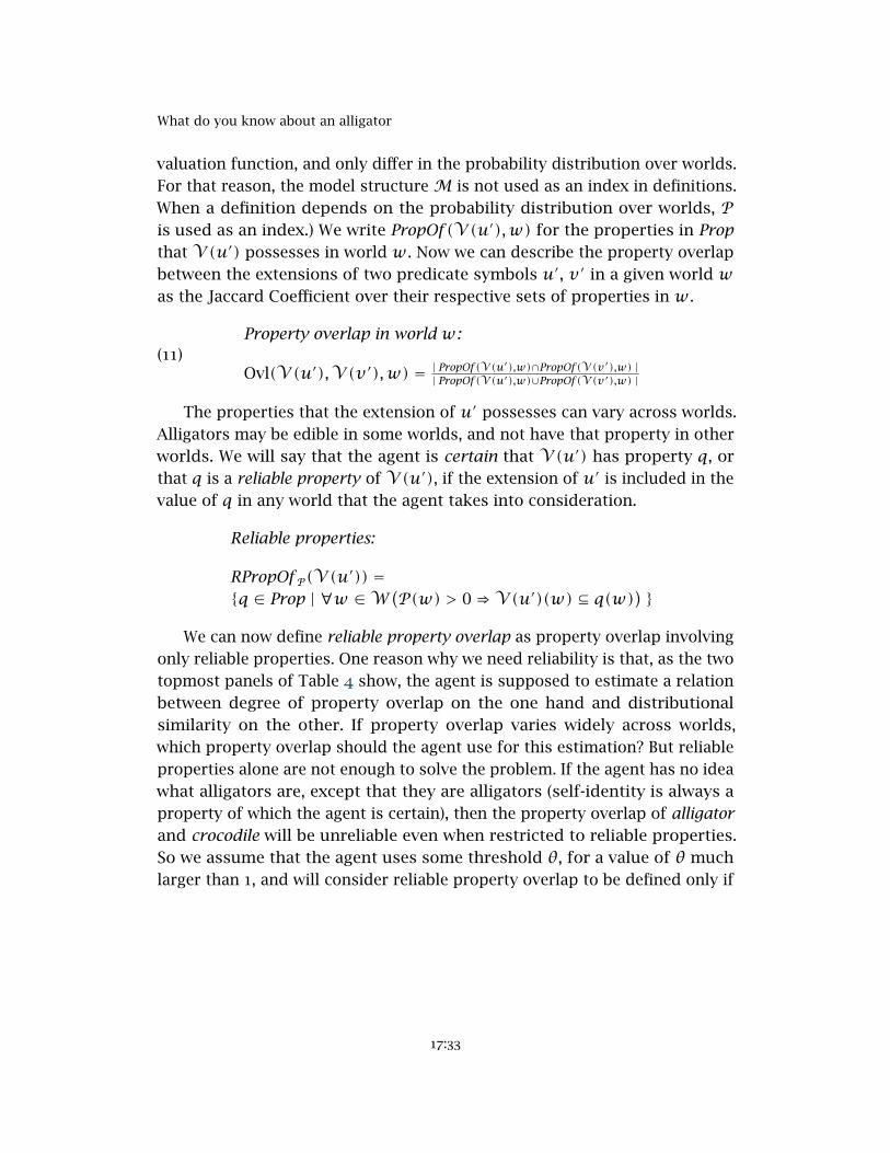
valuation function, and only differ in the probability distribution over worlds.For that reason, the model structureM is not used as an index in definitions.When a definition depends on the probability distribution over worlds, Pis used as an index.) We write PropOf (V (u′),w) for the properties in Propthat V (u′) possesses in world w. Now we can describe the property overlapbetween the extensions of two predicate symbols u′, v ′ in a given world was the Jaccard Coefficient over their respective sets of properties in w.
(11)Property overlap in world w:
Ovl(V (u′),V (v ′),w) = | PropOf (V (u′),w)∩PropOf (V (v′),w) || PropOf (V (u′),w)∪PropOf (V (v′),w) |
The properties that the extension of u′ possesses can vary across worlds.Alligators may be edible in some worlds, and not have that property in otherworlds. We will say that the agent is certain that V (u′) has property q, orthat q is a reliable property of V (u′), if the extension of u′ is included in thevalue of q in any world that the agent takes into consideration.
Reliable properties:
RPropOf P(V (u′)) ={q ∈ Prop | ∀w ∈W
(P(w) > 0⇒ V (u′)(w) ⊆ q(w)
)}
We can now define reliable property overlap as property overlap involvingonly reliable properties. One reason why we need reliability is that, as the twotopmost panels of Table 4 show, the agent is supposed to estimate a relationbetween degree of property overlap on the one hand and distributionalsimilarity on the other. If property overlap varies widely across worlds,which property overlap should the agent use for this estimation? But reliableproperties alone are not enough to solve the problem. If the agent has no ideawhat alligators are, except that they are alligators (self-identity is always aproperty of which the agent is certain), then the property overlap of alligatorand crocodile will be unreliable even when restricted to reliable properties.So we assume that the agent uses some threshold θ, for a value of θ muchlarger than 1, and will consider reliable property overlap to be defined only if
17:33
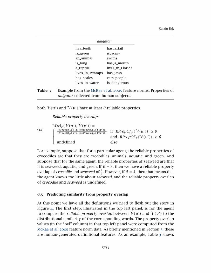
Katrin Erk
alligator
has_teeth has_a_tail
is_green is_scary
an_animal swims
is_long has_a_mouth
a_reptile lives_in_Florida
lives_in_swamps has_jaws
has_scales eats_people
lives_in_water is_dangerous
Table 3 Example from the McRae et al. 2005 feature norms: Properties ofalligator collected from human subjects.
both V (u′) and V (v ′) have at least θ reliable properties.
(12)
Reliable property overlap:
ROvlP(V (u′),V (v ′)) =| RPropOf P(V (u′))∩RPropOf P(V (v′)) || RPropOf P(V (u′))∪RPropOf P(V (v′)) |
if |RPropOf P(V (u′))| ≥ θand |RPropOf P(V (v ′))| ≥ θ
undefined else
For example, suppose that for a particular agent, the reliable properties ofcrocodiles are that they are crocodiles, animals, aquatic, and green. Andsuppose that for the same agent, the reliable properties of seaweed are thatit is seaweed, aquatic, and green. If θ = 3, then we have a reliable propertyoverlap of crocodile and seaweed of 25 . However, if θ = 4, then that means thatthe agent knows too little about seaweed, and the reliable property overlapof crocodile and seaweed is undefined.
6.5 Predicting similarity from property overlap
At this point we have all the definitions we need to flesh out the story inFigure 4. The first step, illustrated in the top left panel, is for the agentto compare the reliable property overlap between V (u′) and V (v ′) to thedistributional similarity of the corresponding words. The property overlapvalues (in the “ovl” column) in that top left panel were computed from theMcRae et al. 2005 feature norm data. As briefly mentioned in Section 3, theseare human-generated definitional features. As an example, Table 3 shows
17:34
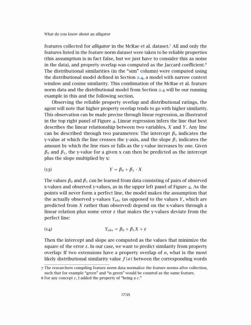
What do you know about an alligator
features collected for alligator in the McRae et al. dataset.7 All and only thefeatures listed in the feature norm dataset were taken to be reliable properties(this assumption is in fact false, but we just have to consider this as noisein the data), and property overlap was computed as the Jaccard coefficient.8
The distributional similarities (in the “sim” column) were computed usingthe distributional model defined in Section 2.4, a model with narrow contextwindow and cosine similarity. This combination of the McRae et al. featurenorm data and the distributional model from Section 2.4 will be our runningexample in this and the following section.
Observing the reliable property overlap and distributional ratings, theagent will note that higher property overlap tends to go with higher similarity.This observation can be made precise through linear regression, as illustratedin the top right panel of Figure 4. Linear regression infers the line that bestdescribes the linear relationship between two variables, X and Y . Any linecan be described through two parameters: The intercept β0 indicates they-value at which the line crosses the y-axis, and the slope β1 indicates theamount by which the line rises or falls as the y-value increases by one. Givenβ0 and β1, the y-value for a given x can then be predicted as the interceptplus the slope multiplied by x:
(13) Y = β0 + β1 ·X
The values β0 and β1 can be learned from data consisting of pairs of observedx-values and observed y-values, as in the upper left panel of Figure 4. As thepoints will never form a perfect line, the model makes the assumption thatthe actually observed y-values Yobs (as opposed to the values Y , which arepredicted from X rather than observed) depend on the x-values through alinear relation plus some error ε that makes the y-values deviate from theperfect line:
(14) Yobs = β0 + β1X + ε
Then the intercept and slope are computed as the values that minimize thesquare of the error ε. In our case, we want to predict similarity from propertyoverlap: If two extensions have a property overlap of o, what is the mostlikely distributional similarity value f(o) between the corresponding words
7 The researchers compiling feature norm data normalize the feature norms after collection,such that for example “green” and “is green” would be counted as the same feature.
8 For any concept c, I added the property of “being a c.”
17:35
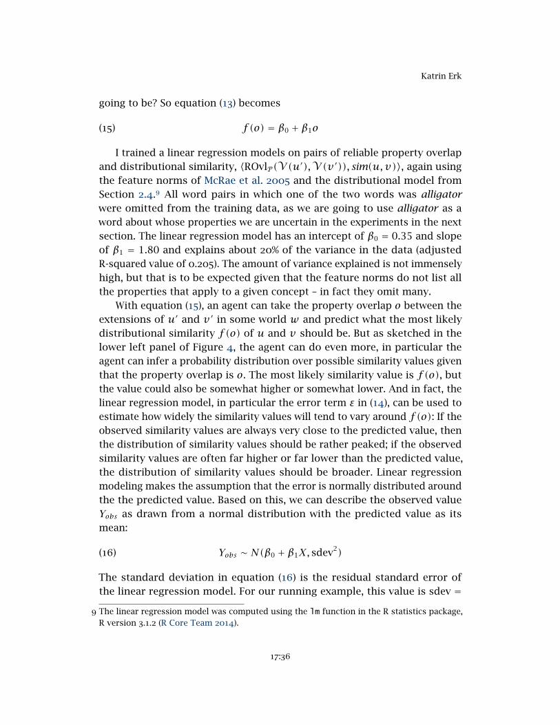
Katrin Erk
going to be? So equation (13) becomes
(15) f(o) = β0 + β1o
I trained a linear regression models on pairs of reliable property overlapand distributional similarity, 〈ROvlP(V (u′),V (v ′)), sim(u,v)〉, again usingthe feature norms of McRae et al. 2005 and the distributional model fromSection 2.4.9 All word pairs in which one of the two words was alligatorwere omitted from the training data, as we are going to use alligator as aword about whose properties we are uncertain in the experiments in the nextsection. The linear regression model has an intercept of β0 = 0.35 and slopeof β1 = 1.80 and explains about 20% of the variance in the data (adjustedR-squared value of 0.205). The amount of variance explained is not immenselyhigh, but that is to be expected given that the feature norms do not list allthe properties that apply to a given concept – in fact they omit many.
With equation (15), an agent can take the property overlap o between theextensions of u′ and v ′ in some world w and predict what the most likelydistributional similarity f(o) of u and v should be. But as sketched in thelower left panel of Figure 4, the agent can do even more, in particular theagent can infer a probability distribution over possible similarity values giventhat the property overlap is o. The most likely similarity value is f(o), butthe value could also be somewhat higher or somewhat lower. And in fact, thelinear regression model, in particular the error term ε in (14), can be used toestimate how widely the similarity values will tend to vary around f(o): If theobserved similarity values are always very close to the predicted value, thenthe distribution of similarity values should be rather peaked; if the observedsimilarity values are often far higher or far lower than the predicted value,the distribution of similarity values should be broader. Linear regressionmodeling makes the assumption that the error is normally distributed aroundthe the predicted value. Based on this, we can describe the observed valueYobs as drawn from a normal distribution with the predicted value as itsmean:
(16) Yobs ∼ N(β0 + β1X, sdev2)
The standard deviation in equation (16) is the residual standard error ofthe linear regression model. For our running example, this value is sdev =
9 The linear regression model was computed using the lm function in the R statistics package,R version 3.1.2 (R Core Team 2014).
17:36
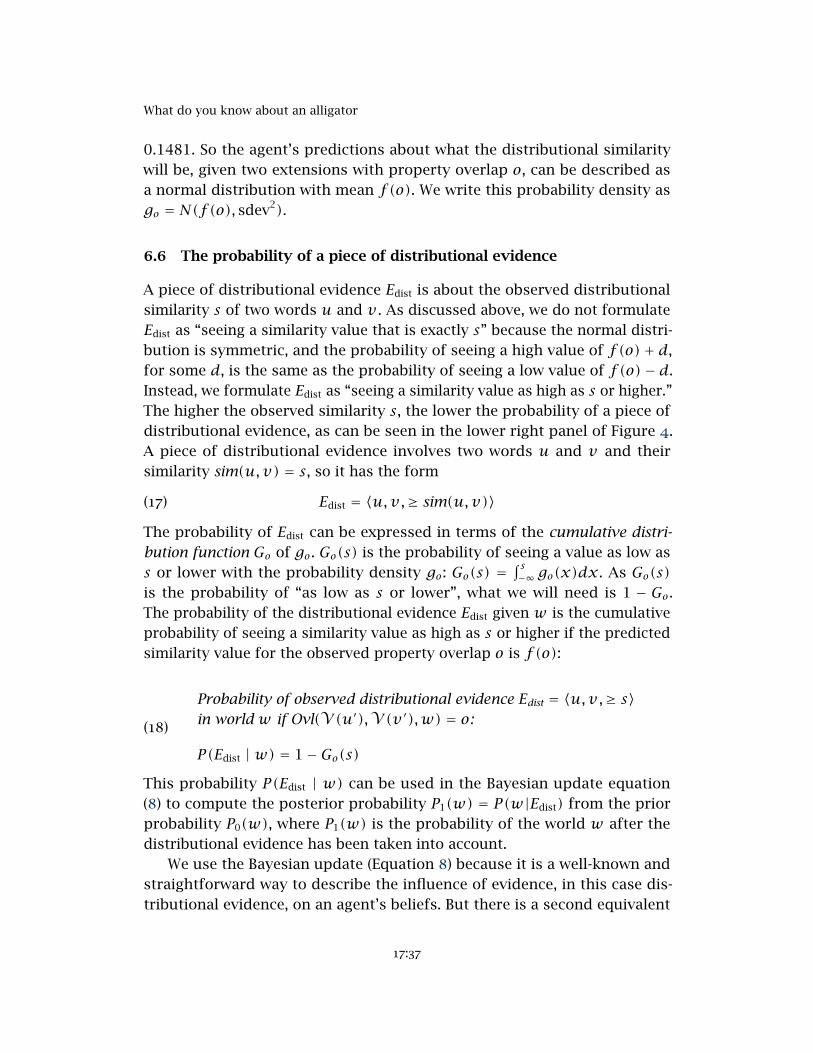
What do you know about an alligator
0.1481. So the agent’s predictions about what the distributional similaritywill be, given two extensions with property overlap o, can be described asa normal distribution with mean f(o). We write this probability density asgo = N(f(o), sdev2).
6.6 The probability of a piece of distributional evidence
A piece of distributional evidence Edist is about the observed distributionalsimilarity s of two words u and v . As discussed above, we do not formulateEdist as “seeing a similarity value that is exactly s” because the normal distri-bution is symmetric, and the probability of seeing a high value of f(o)+ d,for some d, is the same as the probability of seeing a low value of f(o)− d.Instead, we formulate Edist as “seeing a similarity value as high as s or higher.”The higher the observed similarity s, the lower the probability of a piece ofdistributional evidence, as can be seen in the lower right panel of Figure 4.A piece of distributional evidence involves two words u and v and theirsimilarity sim(u,v) = s, so it has the form
(17) Edist = 〈u,v,≥ sim(u,v)〉
The probability of Edist can be expressed in terms of the cumulative distri-bution function Go of go. Go(s) is the probability of seeing a value as low ass or lower with the probability density go: Go(s) =
∫ s−∞ go(x)dx. As Go(s)
is the probability of “as low as s or lower”, what we will need is 1 − Go.The probability of the distributional evidence Edist given w is the cumulativeprobability of seeing a similarity value as high as s or higher if the predictedsimilarity value for the observed property overlap o is f(o):
(18)
Probability of observed distributional evidence Edist = 〈u,v,≥ s〉in world w if Ovl(V (u′),V (v ′),w) = o:
P(Edist | w) = 1−Go(s)
This probability P(Edist | w) can be used in the Bayesian update equation(8) to compute the posterior probability P1(w) = P(w|Edist) from the priorprobability P0(w), where P1(w) is the probability of the world w after thedistributional evidence has been taken into account.
We use the Bayesian update (Equation 8) because it is a well-known andstraightforward way to describe the influence of evidence, in this case dis-tributional evidence, on an agent’s beliefs. But there is a second equivalent
17:37
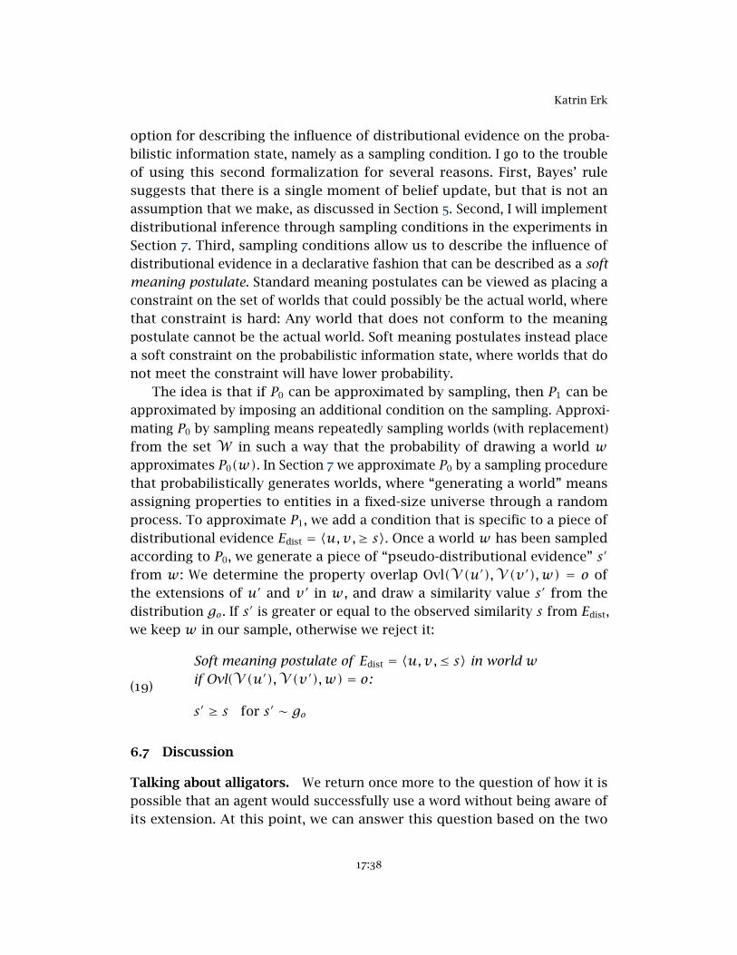
Katrin Erk
option for describing the influence of distributional evidence on the proba-bilistic information state, namely as a sampling condition. I go to the troubleof using this second formalization for several reasons. First, Bayes’ rulesuggests that there is a single moment of belief update, but that is not anassumption that we make, as discussed in Section 5. Second, I will implementdistributional inference through sampling conditions in the experiments inSection 7. Third, sampling conditions allow us to describe the influence ofdistributional evidence in a declarative fashion that can be described as a softmeaning postulate. Standard meaning postulates can be viewed as placing aconstraint on the set of worlds that could possibly be the actual world, wherethat constraint is hard: Any world that does not conform to the meaningpostulate cannot be the actual world. Soft meaning postulates instead placea soft constraint on the probabilistic information state, where worlds that donot meet the constraint will have lower probability.
The idea is that if P0 can be approximated by sampling, then P1 can beapproximated by imposing an additional condition on the sampling. Approxi-mating P0 by sampling means repeatedly sampling worlds (with replacement)from the set W in such a way that the probability of drawing a world wapproximates P0(w). In Section 7 we approximate P0 by a sampling procedurethat probabilistically generates worlds, where “generating a world” meansassigning properties to entities in a fixed-size universe through a randomprocess. To approximate P1, we add a condition that is specific to a piece ofdistributional evidence Edist = 〈u,v,≥ s〉. Once a world w has been sampledaccording to P0, we generate a piece of “pseudo-distributional evidence” s′
from w: We determine the property overlap Ovl(V (u′),V (v ′),w) = o ofthe extensions of u′ and v ′ in w, and draw a similarity value s′ from thedistribution go. If s′ is greater or equal to the observed similarity s from Edist,we keep w in our sample, otherwise we reject it:
(19)
Soft meaning postulate of Edist = 〈u,v,≤ s〉 in world wif Ovl(V (u′),V (v ′),w) = o:
s′ ≥ s for s′ ∼ go
6.7 Discussion
Talking about alligators. We return once more to the question of how it ispossible that an agent would successfully use a word without being aware ofits extension. At this point, we can answer this question based on the two
17:38
What do you know about an alligator
different definitions of uncertainty in Section 6.3. An agent may be unable topoint out an alligator, in the sense that the extensions of alligator′ vary widelyacross the worlds that the agent takes into consideration (which I definedabove as worlds that have non-zero probability in the agent’s informationstate), and the agent can still be absolutely certain that all alligators areanimals, in the sense that the extension of alligator′ is a subset of theextension of animal′ in all worlds that the agent takes into consideration.In that case, the probability of “all alligators are animals” in the agent’sprobabilistic information state is 1, and the agent can confidently makestatements based on the fact that alligators are animals. The same holds forbanyan trees and elms (two examples mentioned in the introduction).
Suppose I am unable to point out an alligator in a zoo, but I am certain thatalligators are animals, and I make statements about alligators based on myinformation state. This creates distributional data that other speakers mightwant to use to learn about word meaning. And in fact if these other speakersnow want to learn about properties of alligators, they can confidently usethe distributional data that I produced, even though I have no idea about theextension of alligator′: If I am certain that alligators are animals, this will bereflected in the verbs and modifiers that I apply to the word alligator, whichin turn will create good data for other speakers to learn from.
Distributional information and formal semantics, loosely coupled throughinference. In this section I have proposed a mechanism for integratingdistributional property inference with formal semantics. This mechanismcouples two different formalisms loosely through probabilistic inference, so itis not a single unified model. And in fact I would say that the eventual aim ofan integration of formal semantics with distributional information would notnecessarily have to be a unified model. Meaning is a complex phenomenon.It involves a notion of truth and grounding, and formal semantics capturesthat well. In this paper I have argued that meaning can also be learned fromobserved use in a community of speakers, which is here represented distri-butionally. And this observed use is not centrally about truth: Useful lexicalinformation can be learned from some non-factual statements. For example,from “Alligators love to eat bananas” an agent can infer that alligators arelikely to be animate (as they can be the subject of eat). So as truth is notcentral to distributional data, it makes sense to represent it differently.
17:39
Katrin Erk
Cognitive plausibility of the model? In this section I have proposed anapproach for how distributional data could be used to influence an agent’sinformation state. Now I briefly turn to the question of whether it would beplausible for a human agent to use distributional data (which is not the sameas to prove that human agents use distributional data; I am not sure thatthe latter would be possible.) The strongest and most well-known argumentthat speakers do use distributional information was made by Landauer &Dumais (1997), who proposed distributional models as “a solution to Plato’sproblem”. This is the question of how humans can possibly acquire thelarge vocabulary that they command, and Landauer and Dumais’ answer isthat humans use contextual clues to learn the meaning of words that theyobserve in linguistic input. Some experimental support for the hypothesis ofdistributional word learning comes from McDonald & Ramscar (2001). Theyuse context to influence the perceived meaning of either marginally familiarwords or made-up words, with a highly significant effect on subsequentsimilarity ratings.
Another argument is that many phenomena in semantics seem to involvegradedness and that distributional models with their graded notion of simi-larity provide a mechanism to explain how humans are able to make suchgraded judgments. This argument can be found in van Eijck & Lappin 2012,though they reject distributional models in the end. Synonymy is an exampleof a phenomenon that seems to involve gradedness: Instead of absolutesynonymy, we find near-synonymy of words that are often substitutable butstill differ in nuances of meaning (Edmonds & Hirst 2002). Polysemy alsoseems to come in degrees, with different uses of a word differing in theirperceived similarity (Brown 2008, Erk, McCarthy & Gaylord 2013). However,distributional similarity of observed textual contexts is not the only possiblesource for graded semantic judgments. Other possibilities include similarityof semantic feature representations, or a probabilistic match between anentity or situation on the one hand and a label on the other hand (Cooperet al. 2014). Still, it is possible that distributional similarity would be one ofthe mechanisms involved.
A third argument, proposed by Baroni, Bernardi & Zamparelli (2014), issimply that distributional evidence is available in ample amounts and it isdemonstrably useful, so it stands to reason that humans would make use ofit.
Taken together, these arguments from the literature make the case that itis reasonable to assume that speakers make use of distributional evidence.
17:40
What do you know about an alligator
They do not prove that speakers necessarily use this kind of information, butas I said above, this stronger argument is not one I am even attempting tomake.
The converse question is whether there are any reasons why humanscannot make use of any distributional clues. There does not seem to beany work that argues this point, but there are many papers, for instancevan Eijck & Lappin 2012, that argue a weaker point, namely that not all ofhuman language processing can be distributional. Lenci (2008) lists threemain reasons: that distributional models lack compositionality, do not sup-port inference, and cannot provide reference. Although these three problemsremain difficult for distributional models, there has been considerable workon all of them since Lenci’s paper appeared. Concerning compositionality, thecompositional construction of distributional phrase representations is cur-rently an active area of research (Landauer & Dumais 1997, Mitchell & Lapata2010, Baroni & Zamparelli 2010, Coecke, Sadrzadeh & Clark 2011, Grefenstette& Sadrzadeh 2011, Socher et al. 2012, Baroni, Bernardi & Zamparelli 2014).We have discussed the topic of distributional inference in Section 3. Andconcerning reference, there has been work on vector space representationsthat integrate textual, visual, and conceptual information (Feng & Lapata2010, Andrews, Vigliocco & Vinson 2009, Bruni et al. 2012) and on mappingbetween textual and visual spaces (Lazaridou, Bruni & Baroni 2014).
Summing up these arguments that aim to show that not all of humanlanguage processing can be distributional, what they mostly show is thatdistributional models are a moving target. The field is currently making fastprogress, such that it is hard to say which constraints on the expressivepower of distributional models will turn out to be fundamental and whichwill be overcome by future models. Still, the picture that emerges from thecurrent limitations of distributional models is that distributional evidence isconceivable as part of a human language processing apparatus, but not all ofit. This is also the view that I take in this paper.
7 Learning about alligators: three experiments
This section reports on three proof of concept experiments that showcasethe mechanism from the previous section. The experiments are kept simplein order to better illustrate the properties of the model: In the first twoexperiments we study how the model learns from one single word, at eitherhigh or medium distributional similarity to the unknown word. In the third
17:41
Katrin Erk
experiment we test how the model learns from two different words at thesame time.
We focus on the three example sentences from the introduction, repeatedhere for convenience:
ϕ1: All alligators are dangerous.
ϕ2: All alligators are edible.
ϕ3: All alligators are animals.
We assume an agent who is uncertain about the properties of alligators,but certain about the properties of crocodiles and trouts. Among other things,the agent is certain that crocodiles are dangerous, trouts are edible, and bothcrocodiles and trouts are animals, in the sense of Section 6.3: In all worlds thatthe agent takes into consideration (to which they assign nonzero probability),the extension of crocodile′ is a subset of the extension of dangerous′, andanalogously for the other properties.
In the first experiment, we use sentence ϕ1 to test how distributional sim-ilarity of alligator and crocodile influences the degree of the agent’s certaintythat alligators are dangerous. The second experiment tests the influence ofthe distributional similarity of alligator and trout on the probability that theagent ascribes to ϕ2. The difference between the first two experiments isthat the distributional similarity of alligator to crocodile is very high whilethe similarity to trout is only moderate. With sentence ϕ3 we test whetherevidence (about alligators potentially being animals) can accumulate if wehave distributional similarity ratings of alligator to both crocodile and trout.But let me point out again that the evidence in all three cases is probabilisticand noisy. We will not be able to conclude with certainty that all alligatorsare dangerous, or even that all alligators are animals. And that is as it shouldbe: We do not want to draw inferences with complete certainty based on evi-dence that does not provide complete certainty. What I aim to show instead isthat the distributional evidence significantly affects the agent’s probabilisticinformation state, in particular that evidence about distributional similaritycan bring the agent to consider it more likely that alligators have propertiesthat crocodiles and trouts also possess. That is the measuring stick by whichwe will judge whether we have been able to show that distributional evidenceis useful.
Throughout this section, we use sampling to approximate the prior prob-ability distribution P0 over possible worlds. And we use sampling constraints
17:42
What do you know about an alligator
in the form of the soft meaning postulates in Equation (19) to sample fromthe posterior P1 instead of P0, where P1 is the probability distribution overpossible worlds that takes the distributional evidence into account.
To obtain the numbers for our experiments, we again use the McRae et al.2005 feature norms as property lists, we use the distributional model fromSection 2.4, and we use the linear regression model from the previous sectionthat predicted distributional similarity from property overlap.
Experiment 1: Are alligators dangerous? For this experiment, we assumethat we know a lot about crocodiles: they are animals, dangerous, and scaly –and they are crocodiles. Of alligators, we only know that they are alligators.(Note that we do not have to assume that we know all properties of crocodiles.In particular we do not have to assume that we know whether they arealligators.) What we want to know in this experiment is how the distributionalsimilarity of alligator and crocodile, which in our distributional model is 0.93,will affect the degree of property uncertainty that we have about alligators.In particular, we will measure the probability of sentence ϕ1 above, “allalligators are dangerous”, according to the prior probability distribution P0and the posterior P1.
To do sampling, we make use of the fact that for a small, finite domainsize, it is possible to explicitly generate worlds (Richardson & Domingos2006, Goodman & Lassiter 2014). We generate a world by probabilisticallyassigning properties to entities in a fixed-size universe. By repeatedly gen-erating worlds through this generative model, we approximate P0 throughsampling. Generative models are typically described in terms of a generativestory, a list of instructions on how the relevant data is generated accordingto the generative model. Often, this generative story is not carried out andis just an abstract characterization of the model. In our case, the generativestory is also a high-level description of the program that was used to generatethe worlds in practice. The generative story looks like this.
• Fix a domain size n for the universe U. We use n = 10.
• Fix a finite collection of predicate symbols. We use alligator′, animal′,crocodile′, dangerous′, scaly′.
• Fix an extension membership probability pext. We use pext = 0.5.
• For each predicate symbol q′ ∈ {alligator′, crocodile′}:
17:43
Katrin Erk
– For each entity e in the domain: Flip a coin with bias pext todetermine whether e is in the extension of q′ or not.
• For each predicate symbol q′ ∈ {animal′, dangerous′, scaly′}:
– For each entity e in the domain: If e is in the extension ofcrocodile′, then e is also in the extension of q′. (This way wemake sure that all crocodiles are animals, dangerous, and scaly.)
If e is not in the extension of crocodile′, flip a coin with bias pextto determine whether e is in the extension of q′.
In all worlds generated in this way, all crocodiles will be animals, danger-ous, and scaly, because these subset relations are enforced by the generativeprocess. But the worlds that we generate will differ in whether all alligatorsare animals, dangerous, or scaly, because the probabilistic process doesnot enforce any particular relations between these properties. So the agentwhose probabilistic information state we model has no uncertainty aboutthe properties of crocodiles (except about whether they are alligators), but isquite uncertain about the properties of alligators. Note that this generativemodel specifies the degree of uncertainty about properties that the agenthas, but does not specify whether the agent has any uncertainty about exten-sions, and in fact even the extension of crocodile is allowed to vary randomlyacross worlds. This is because our model influences (and is influenced by)uncertainty about properties, but not (at least not directly) uncertainty aboutextensions.
We can estimate the probability of a sentence ϕ under the probabilitydistribution P0 by probabilistically generating worlds with the generativemodel and counting in how many of the generated worlds ϕ is true. Butbecause we know how worlds are generated by the generative model, wecan analytically determine the probabilities of some sentences of interestunder P0. The probability of “all crocodiles are dangerous” is 1, because thegenerative process is such that any entity that is a crocodile will also be inthe extension of dangerous′. Next, we consider the sentence “all alligatorsare crocodiles.” If an entity is an alligator, its probability of being a crocodileas well is pext = 0.5 (as the agent that we are modeling does not know anybetter), so the probability that any given entity will be both a crocodile andan alligator is 0.5 · 0.5 = 0.25. The sentence “all alligators are crocodiles”is true in a world if every entity is either not an alligator (which is the casewith probability 0.5) or both an alligator and a crocodile (which is the case
17:44
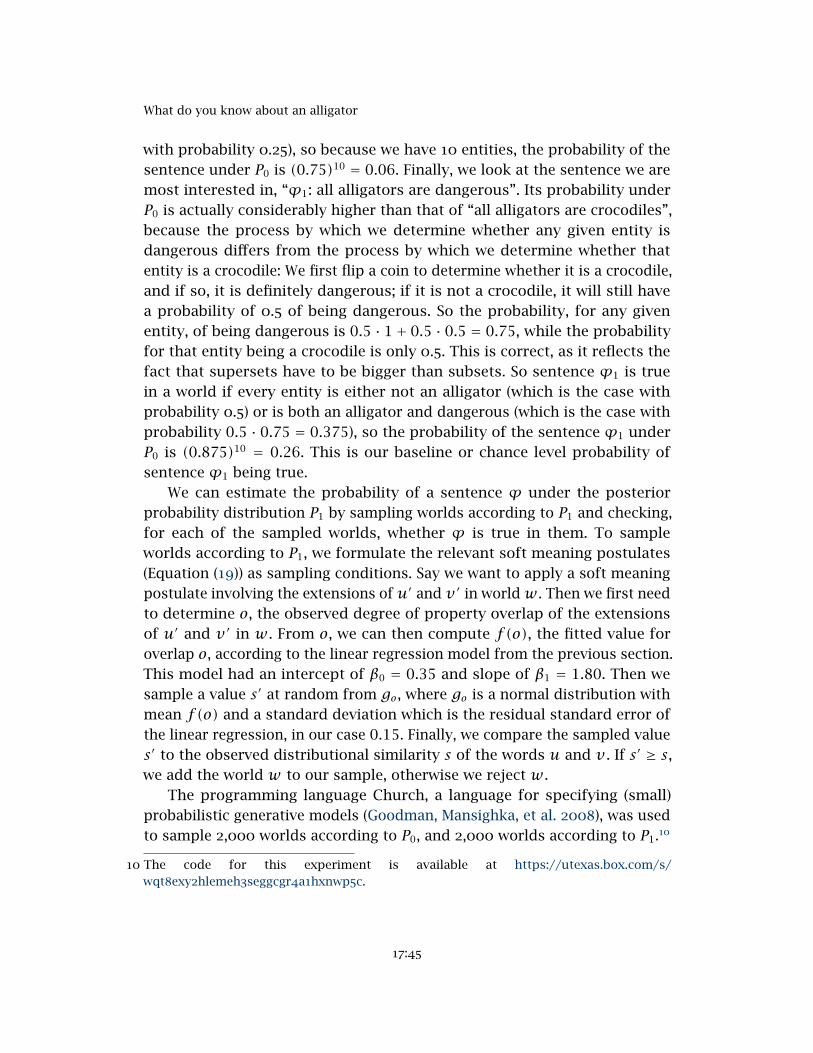
What do you know about an alligator
with probability 0.25), so because we have 10 entities, the probability of thesentence under P0 is (0.75)10 = 0.06. Finally, we look at the sentence we aremost interested in, “ϕ1: all alligators are dangerous”. Its probability underP0 is actually considerably higher than that of “all alligators are crocodiles”,because the process by which we determine whether any given entity isdangerous differs from the process by which we determine whether thatentity is a crocodile: We first flip a coin to determine whether it is a crocodile,and if so, it is definitely dangerous; if it is not a crocodile, it will still havea probability of 0.5 of being dangerous. So the probability, for any givenentity, of being dangerous is 0.5 · 1+ 0.5 · 0.5 = 0.75, while the probabilityfor that entity being a crocodile is only 0.5. This is correct, as it reflects thefact that supersets have to be bigger than subsets. So sentence ϕ1 is truein a world if every entity is either not an alligator (which is the case withprobability 0.5) or is both an alligator and dangerous (which is the case withprobability 0.5 · 0.75 = 0.375), so the probability of the sentence ϕ1 underP0 is (0.875)10 = 0.26. This is our baseline or chance level probability ofsentence ϕ1 being true.
We can estimate the probability of a sentence ϕ under the posteriorprobability distribution P1 by sampling worlds according to P1 and checking,for each of the sampled worlds, whether ϕ is true in them. To sampleworlds according to P1, we formulate the relevant soft meaning postulates(Equation (19)) as sampling conditions. Say we want to apply a soft meaningpostulate involving the extensions of u′ and v ′ in worldw . Then we first needto determine o, the observed degree of property overlap of the extensionsof u′ and v ′ in w. From o, we can then compute f(o), the fitted value foroverlap o, according to the linear regression model from the previous section.This model had an intercept of β0 = 0.35 and slope of β1 = 1.80. Then wesample a value s′ at random from go, where go is a normal distribution withmean f(o) and a standard deviation which is the residual standard error ofthe linear regression, in our case 0.15. Finally, we compare the sampled values′ to the observed distributional similarity s of the words u and v . If s′ ≥ s,we add the world w to our sample, otherwise we reject w.
The programming language Church, a language for specifying (small)probabilistic generative models (Goodman, Mansighka, et al. 2008), was usedto sample 2,000 worlds according to P0, and 2,000 worlds according to P1.10
10 The code for this experiment is available at https://utexas.box.com/s/wqt8exy2hlemeh3seggcgr4a1hxnwp5c.
17:45
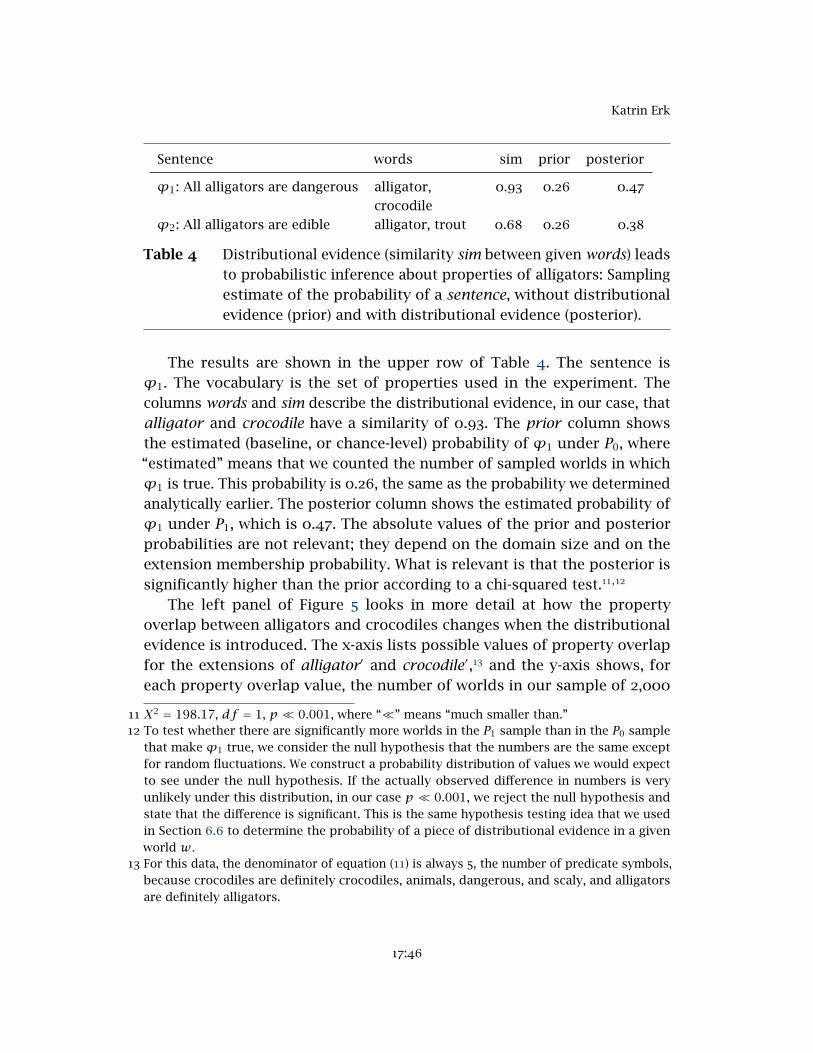
Katrin Erk
Sentence words sim prior posterior
ϕ1: All alligators are dangerous alligator,
crocodile
0.93 0.26 0.47
ϕ2: All alligators are edible alligator, trout 0.68 0.26 0.38
Table 4 Distributional evidence (similarity sim between given words) leadsto probabilistic inference about properties of alligators: Samplingestimate of the probability of a sentence, without distributionalevidence (prior) and with distributional evidence (posterior).
The results are shown in the upper row of Table 4. The sentence isϕ1. The vocabulary is the set of properties used in the experiment. Thecolumns words and sim describe the distributional evidence, in our case, thatalligator and crocodile have a similarity of 0.93. The prior column showsthe estimated (baseline, or chance-level) probability of ϕ1 under P0, where“estimated” means that we counted the number of sampled worlds in whichϕ1 is true. This probability is 0.26, the same as the probability we determinedanalytically earlier. The posterior column shows the estimated probability ofϕ1 under P1, which is 0.47. The absolute values of the prior and posteriorprobabilities are not relevant; they depend on the domain size and on theextension membership probability. What is relevant is that the posterior issignificantly higher than the prior according to a chi-squared test.11,12
The left panel of Figure 5 looks in more detail at how the propertyoverlap between alligators and crocodiles changes when the distributionalevidence is introduced. The x-axis lists possible values of property overlapfor the extensions of alligator′ and crocodile′,13 and the y-axis shows, foreach property overlap value, the number of worlds in our sample of 2,000
11 X2 = 198.17, df = 1, p� 0.001, where “�” means “much smaller than.”12 To test whether there are significantly more worlds in the P1 sample than in the P0 sample
that make ϕ1 true, we consider the null hypothesis that the numbers are the same exceptfor random fluctuations. We construct a probability distribution of values we would expectto see under the null hypothesis. If the actually observed difference in numbers is veryunlikely under this distribution, in our case p� 0.001, we reject the null hypothesis andstate that the difference is significant. This is the same hypothesis testing idea that we usedin Section 6.6 to determine the probability of a piece of distributional evidence in a givenworld w.
13 For this data, the denominator of equation (11) is always 5, the number of predicate symbols,because crocodiles are definitely crocodiles, animals, dangerous, and scaly, and alligatorsare definitely alligators.
17:46
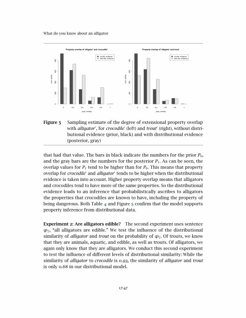
What do you know about an alligator
0 0.2 0.4 0.6 0.8 1
no dist. evidencewith dist. evidence
Property overlap of 'alligator' and 'crocodile'
prop. overlap
num
. wor
lds
0200
400
600
800
0 0.2 0.4 0.6 0.8 1
no dist. evidencewith dist. evidence
Property overlap of 'alligator' and trout'
prop. overlap
num
. wor
lds
0200
400
600
800
Figure 5 Sampling estimate of the degree of extensional property overlapwith alligator′, for crocodile′ (left) and trout′ (right), without distri-butional evidence (prior, black) and with distributional evidence(posterior, gray)
that had that value. The bars in black indicate the numbers for the prior P0,and the gray bars are the numbers for the posterior P1. As can be seen, theoverlap values for P1 tend to be higher than for P0. This means that propertyoverlap for crocodile′ and alligator′ tends to be higher when the distributionalevidence is taken into account. Higher property overlap means that alligatorsand crocodiles tend to have more of the same properties. So the distributionalevidence leads to an inference that probabilistically ascribes to alligatorsthe properties that crocodiles are known to have, including the property ofbeing dangerous. Both Table 4 and Figure 5 confirm that the model supportsproperty inference from distributional data.
Experiment 2: Are alligators edible? The second experiment uses sentenceϕ2, “all alligators are edible.” We test the influence of the distributionalsimilarity of alligator and trout on the probability of ϕ2. Of trouts, we knowthat they are animals, aquatic, and edible, as well as trouts. Of alligators, weagain only know that they are alligators. We conduct this second experimentto test the influence of different levels of distributional similarity: While thesimilarity of alligator to crocodile is 0.93, the similarity of alligator and troutis only 0.68 in our distributional model.
17:47
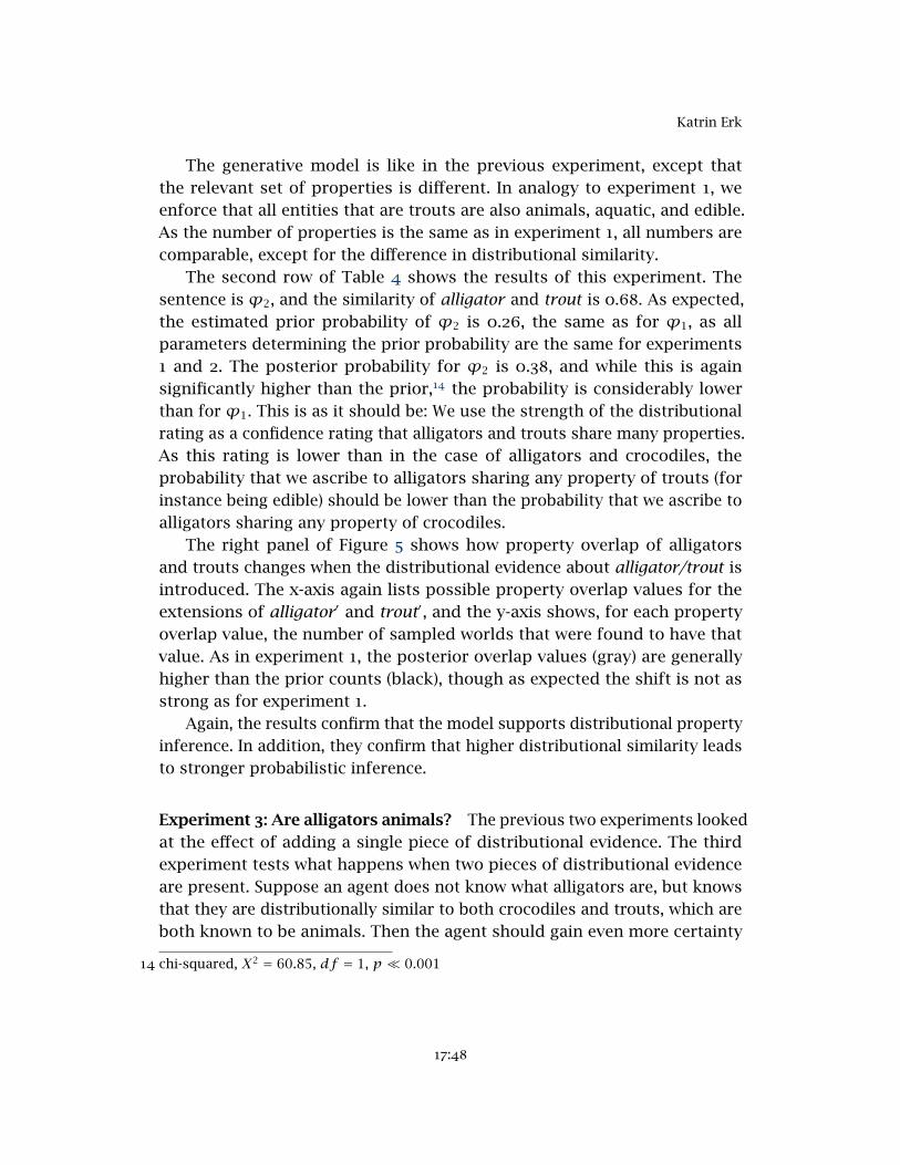
Katrin Erk
The generative model is like in the previous experiment, except thatthe relevant set of properties is different. In analogy to experiment 1, weenforce that all entities that are trouts are also animals, aquatic, and edible.As the number of properties is the same as in experiment 1, all numbers arecomparable, except for the difference in distributional similarity.
The second row of Table 4 shows the results of this experiment. Thesentence is ϕ2, and the similarity of alligator and trout is 0.68. As expected,the estimated prior probability of ϕ2 is 0.26, the same as for ϕ1, as allparameters determining the prior probability are the same for experiments1 and 2. The posterior probability for ϕ2 is 0.38, and while this is againsignificantly higher than the prior,14 the probability is considerably lowerthan for ϕ1. This is as it should be: We use the strength of the distributionalrating as a confidence rating that alligators and trouts share many properties.As this rating is lower than in the case of alligators and crocodiles, theprobability that we ascribe to alligators sharing any property of trouts (forinstance being edible) should be lower than the probability that we ascribe toalligators sharing any property of crocodiles.
The right panel of Figure 5 shows how property overlap of alligatorsand trouts changes when the distributional evidence about alligator/trout isintroduced. The x-axis again lists possible property overlap values for theextensions of alligator′ and trout′, and the y-axis shows, for each propertyoverlap value, the number of sampled worlds that were found to have thatvalue. As in experiment 1, the posterior overlap values (gray) are generallyhigher than the prior counts (black), though as expected the shift is not asstrong as for experiment 1.
Again, the results confirm that the model supports distributional propertyinference. In addition, they confirm that higher distributional similarity leadsto stronger probabilistic inference.
Experiment 3: Are alligators animals? The previous two experiments lookedat the effect of adding a single piece of distributional evidence. The thirdexperiment tests what happens when two pieces of distributional evidenceare present. Suppose an agent does not know what alligators are, but knowsthat they are distributionally similar to both crocodiles and trouts, which areboth known to be animals. Then the agent should gain even more certainty
14 chi-squared, X2 = 60.85, df = 1, p� 0.001
17:48
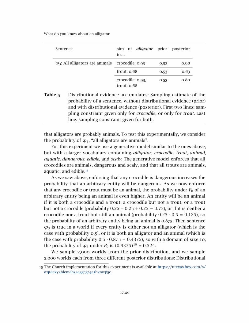
What do you know about an alligator
Sentence sim of alligator
to. . .
prior posterior
ϕ3: All alligators are animals crocodile: 0.93 0.53 0.68
trout: 0.68 0.53 0.63
crocodile: 0.93,
trout: 0.68
0.53 0.80
Table 5 Distributional evidence accumulates: Sampling estimate of theprobability of a sentence, without distributional evidence (prior)and with distributional evidence (posterior). First two lines: sam-pling constraint given only for crocodile, or only for trout. Lastline: sampling constraint given for both.
that alligators are probably animals. To test this experimentally, we considerthe probability of ϕ3, “all alligators are animals”.
For this experiment we use a generative model similar to the ones above,but with a larger vocabulary containing alligator, crocodile, trout, animal,aquatic, dangerous, edible, and scaly. The generative model enforces that allcrocodiles are animals, dangerous and scaly, and that all trouts are animals,aquatic, and edible.15
As we saw above, enforcing that any crocodile is dangerous increases theprobability that an arbitrary entity will be dangerous. As we now enforcethat any crocodile or trout must be an animal, the probability under P0 of anarbitrary entity being an animal is even higher. An entity will be an animalif it is both a crocodile and a trout, a crocodile but not a trout, or a troutbut not a crocodile (probability 0.25+ 0.25+ 0.25 = 0.75), or if it is neither acrocodile nor a trout but still an animal (probability 0.25 · 0.5 = 0.125), sothe probability of an arbitrary entity being an animal is 0.875. Then sentenceϕ3 is true in a world if every entity is either not an alligator (which is thecase with probability 0.5), or it is both an alligator and an animal (which isthe case with probability 0.5 · 0.875 = 0.4375), so with a domain of size 10,the probability of ϕ3 under P0 is (0.9375)10 = 0.524.
We sample 2,000 worlds from the prior distribution, and we sample2,000 worlds each from three different posterior distributions: Distributional
15 The Church implementation for this experiment is available at https://utexas.box.com/s/wqt8exy2hlemeh3seggcgr4a1hxnwp5c.
17:49
Katrin Erk
evidence stating the similarity of alligator and crocodile (but no informationabout similarity to trout), distributional evidence only for alligator/trout,and distributional evidence for both alligator/crocodile and alligator/trout.The results are shown in Table 5. The estimated probability of ϕ3 under theprior probability distribution is shown in the “prior” column. At 0.53, it isreasonably close to the analytically determined value of 0.524. The estimatedprobabilities ofϕ3 under the three different posterior distributions are shownin the “posterior” column: 0.68 when we have distributional evidence aboutalligator/crocodile only, 0.63 with alligator/trout only, and 0.8 when we knowthe similarity of alligator to both crocodile and trout. The posterior probabilityis significantly higher than the prior in all three conditions.16 Comparingthe first two conditions, we see that as before, the higher distributionalsimilarity of alligator to crocodile than to trout leads to higher certainty ofthe inference. Crucially, when we compare the third condition to the first two,we see that distributional evidence does indeed accumulate, as the posteriorprobability, at 0.8, is significantly higher than in the other conditions.17 So themore types of animals we know that are distributionally similar to alligator,the more certain we will be that alligators are animals as well.18
These results confirm that the model supports accumulating evidence,where the probabilistic inference about a property q becomes stronger themore distributional evidence the agent has about other terms that haveproperty q.
Overall, the three experiments in this section have shown that the modelproposed in this paper lets an agent probabilistically infer properties of anunknown word from distributional evidence. In the prior setting, withoutdistributional evidence, the simulated agent had no knowledge of what prop-
16 Chi-squared tests were again used. For evidence only about crocodile, we have: X2 = 87.92,df = 1, p � 0.0001. For evidence only about trout: X2 = 38.23, df = 1, p � 0.0001. Forevidence about both: X2 = 312.28, df = 1, p � 0.0001. So the differences are significanteven with Bonferroni correction for multiple testing.
17 A chi-squared test was performed to compare the condition with distributional informationabout crocodile only to the condition with distributional information about crocodile andtrout. The result was: X2 = 72.36, df = 1, p� 0.0001.
18 Incidentally, the agent will also infer, based on the distributional similarity of alligator totrout, that alligators may be fish. This is interesting because it shows the interaction betweendistributional evidence and other knowledge: If the agent knows, say from school, thatcrocodiles are definitely reptiles and that reptiles and fish are disjoint, then the agent willgive nonzero probability to some worlds where all alligators are reptiles but not fish, and tosome worlds where all alligators are fish but not reptiles – but zero probability to all worldswhere alligators are both reptiles and fish.
17:50
What do you know about an alligator
erties alligators might have, besides being alligators. When distributionalevidence was taken into account, the probabilistic information state showeda considerably higher likelihood that alligators are dangerous, edible, andanimals (respectively, in the three experiments). The simulated agent wasable to make these probabilistic inferences without explicitly learning abouteither the properties or the extension of alligator. In more detail, experiments1 and 2 have shown that the stronger the distributional evidence, that is,the higher the distributional similarity between alligator and a word u, thestronger the probabilistic inference that alligators have the properties thatu is known to have. Experiment 3 has shown that the model accumulatesevidence from distributional similarity to multiple words.
8 Related work: Distributional information and formal semantics
In this section, I discuss existing papers that link distributional models toeither logical form as it is used in computational linguistics, or to semantictheory. There are not many papers that propose such a link, and the papersthat exist differ widely in their backgrounds, their goals, and in the proposedmodels. So my aim in this section is not to unify all those papers into a singlestory, but to showcase the current variety in people’s thinking about thetopic.
In computational linguistics, Beltagy et al. 2013 and Lewis & Steedman 2013extend logical form representations of sentence meaning with distributionalinformation. Their aim is to address polysemy and to obtain additionalinference rules beyond those that can be extracted from manually createdlexical resources. In particular the approach that we proposed in Beltagy etal. is related to this paper. In Beltagy et al., we computed the probabilities oftruth assignments based on the weights of distributional evidence. But weused a heuristic to get from distributional weights to probabilities of truthassignments, while the current paper proposes a principled mechanism forthe influence of distributional evidence on the probability of a world. Lewis &Steedman 2013 uses distributional information to induce word senses and todecide on the preferred sense in a given context, but at the sentence levelthey use standard first-order logic.
The underlying question in Erk 2013 is how inferential information en-coded distributionally could be linked to a model-theoretic semantics. Isuggested that distributional representations are modeling mental concepts,as they have successfully been used to model different phenomena connected
17:51
Katrin Erk
to conceptual representations. I further suggested that intensions are linkedto mental concepts, providing a connection between distributional repre-sentations and model theory. But to make this possible, the paper had todisregard gradedness, one of the core properties of distributional models.Also, the nature of the connection between distributional representations,mental concepts, and intensions was not worked out.
The main aim of Copestake & Herbelot 2013 is to point out a formal con-nection between model theory and distributional semantics, namely throughthe sentences that are true of an entity in the world. They postulate an “idealdistribution” as a distributional model computed from a corpus that consistsof logical forms of all true statements about all entities in the world. Theactual distribution that a speaker perceives is then an approximation of theideal distribution. The approach is elegant in that it reduces distributionalinformation to information on what is true about entities in the world. Itis also interesting in its change of focus from the words that make up thecorpus to the entities that the corpus is about; Herbelot continues the workon individuals and their distributional trace in Herbelot 2015. But the relianceon ideal distributions is a drawback of the approach. Actual distributionsdo not approximate ideal distributions too well. They are noisy and oddlyeclectic. So I feel that it is important to discuss, as I did in this paper, how aspeaker can learn from distributional data that is imperfect in all these ways,and also how noisy distributional information can be integrated with otherknowledge.
Larsson (2015) is interested in learning from perceptual information. Heuses vector space representations, but he uses them not for distributionalbut low-level perceptual information. He defines perceptual meanings asperceptron classifiers operating on the perceptual information, and viewsthese classifiers as intensions. Larsson discusses the connection of his workto distributional approaches, in particular whether his perceptual vectorscould be viewed as distributional. They could: There are distributional modelsthat use perceptual or mixed perceptual and textual dimensions (Andrews,Vigliocco & Vinson 2009, Feng & Lapata 2010, Bruni et al. 2012). Cooper et al.(2014) take the idea further by applying perceptual classifiers to situations,which are abstract objects with associated features that are propositions.As discussed in Section 5, they frame this idea in a probabilistic system oftypes, where situations are assigned types that are propositions, and thisassignment is associated with probabilities.
17:52
What do you know about an alligator
It remains to be seen if in the future there will be convergence on thequestion of how distributional and formal semantics should be linked, andto what end.
9 Conclusion
In this paper I have suggested that (for suitable distributional models) distri-butional similarity signals property overlap. This is possible because distribu-tional evidence keeps track of the predicates that apply to a noun target, andthe selectional constraints of a predicate indicate properties of its argument.Because of this, distributional evidence can be used for property inference: “Idon’t know what an alligator is, but it must be something like a crocodile, soit is probably an animal.”
I have also proposed a mechanism for distributional property inference. Itassumes that an agent has a probabilistic information state that can make useof noisy, incomplete data like distributional data. Based on the observationthat alligator and crocodile have a high distributional similarity, the agentinfers that the two words must have a high property overlap, and adoptsa probabilistic information state that ascribes higher probability to worldsin which this is the case. The mechanism focuses on an agent’s uncertaintyabout properties, not their uncertainty about extensions. I have pointed outthat an agent can be highly certain that alligators are animals without beingcertain about the extension of alligator′, which explains how an agent canuse a word felicitously without being aware of its extension.
This paper takes a first step in the direction of integrating formal se-mantics with distributional information, but at this point there are of coursemany more open questions than solved ones. On the topic of learning wordmeaning from distributional evidence, one obvious question is what happenswhen properties only apply to some but not all entities in an extension. Ifalligators are distributionally similar to crocodiles, then can we draw any con-clusions from the fact that some but not all crocodiles live in zoos? Also, notall of word meaning can be easily described through verbalizable properties.For example, what distinguishes the word skittish from nervous? Andrews,Vigliocco & Vinson (2009) suggest that it is words like crime, justice, andfinance where distributional evidence is most important to word learning.But if the meaning of such words cannot easily be defined through propertylists, then what is an agent learning about them from distributional data?Another question concerns learning from data that is not distributional. For
17:53
Katrin Erk
example, what if an agent has once seen an alligator in the zoo, and has alsoacquired distributional information about these creatures: How do the twoknowledge sources combine?
Polysemy is another big issue to address, learning the meanings of poly-semous words, but also determining the meaning of a polysemous word in aparticular sentence context. It has been suggested that distributional infor-mation can help on this task (Erk 2010, McNally & Boleda 2014), and maybethe mechanism from this paper can prove useful for addressing polysemyas well. A probabilistic framework, like the one introduced in this paper,should be useful in characterizing word meaning in context, as differencesin meaning seem to come in degrees (Brown 2008, Erk, McCarthy & Gaylord2013). And maybe the task of describing what a word means in a particularsentence can be framed as property inference, namely inferring the mostrelevant properties of a word in a given context.
Another issue that needs further work is the probabilistic inference frame-work. As discussed in Section 5, the probabilistic logic that we use is problem-atic in that it is currently not clear how to extend it to infinitely many worlds.One way to address this is to find a way to extend it, a direction that Clarke& Keller (2015) take; another is to pursue a formulation in a situation-basedframework like that of Cooper et al. (2014) or Goodman & Lassiter (2014).
Finally, there is a need for more research on distributional models forproperty inference, to develop efficient models beyond the initial approachesproposed by Johns & Jones (2012), Fagarasan, Vecchi & Clark (2015), Herbelot& Vecchi (2015) and Gupta et al. (2015) and to see what kinds of propertiescan be reliably learned and whether verb properties can be learned as well asnoun properties.
The aim of this paper was to argue for distributional similarity as prop-erty overlap, and to provide a first simple model for how agents may usedistributional evidence in a probabilistic framework. I hope that this modelwill prove to be extensible to addressing some of these open questions in thefuture.
References
Agirre, Eneko, Enrique Alfonseca, Keith Hall, Jana Kravalova, Marius Pasca &Aitor Soroa. 2009. A study on similarity and relatedness using distribu-tional and WordNet-based approaches. In North American Chapter of theAssociation for Computational Linguistics: Human language technologies
17:54
What do you know about an alligator
(NAACL HLT). Boulder, CO. http://aclweb.org/anthology/N/N09/N09-1003.pdf.
Almuhareb, Abdulrahman & Massimo Poesio. 2004. Attribute-based andvalue-based clustering: An evaluation. In Conference on empirical methodsin natural language processing (EMNLP), 158–165. http://aclweb.org/anthology/W/W04/W04-3221.pdf.
Almuhareb, Abdulrahman & Massimo Poesio. 2005. Finding concept attributesin the web using a parser. In Proceedings of the corpus linguistics confer-ence. Birmingham. http://www.birmingham.ac.uk/Documents/college-artslaw/corpus/conference-archives/2005-journal/Thewebasacorpus/cl133papalmuhareb.pdf.
Andrews, Mark, Gabriella Vigliocco & David Vinson. 2009. Integrating expe-riential and distributional data to learn semantic representations. Psy-chological Review 116(3). 463–498. http://dx.doi.org/10.1037/a0016261.http://www.mjandrews.net/papers/andrews.psychrev.2009.pdf.
Baroni, Marco, Raffaella Bernardi & Roberto Zamparelli. 2014. Frege in space:A program for compositional distributional semantics. Linguistic Issuesin Language Technology 9(6). 5–110. http://elanguage.net/journals/lilt/article/view/3746.
Baroni, Marco, Silvia Bernardini, Adriano Ferraresi & Eros Zanchetta. 2009.The WaCky wide web: a collection of very large linguistically processedweb-crawled corpora. Language Resources and Evaluation 43(3). 209–226.http://dx.doi.org/10.1007/s10579-009-9081-4. http://clic.cimec.unitn.it/marco/publications/wacky-lrej.pdf.
Baroni, Marco, Georgiana Dinu & Germán Kruszewski. 2014. Don’t count, pre-dict! A systematic comparison of context-counting vs. context-predictingsemantic vectors. In 52nd annual meeting of the Association for Computa-tional Linguistics (ACL). http://aclweb.org/anthology/P/P14/P14-1023.pdf.
Baroni, Marco & Alessandro Lenci. 2010. Distributional memory: A generalframework for corpus-based semantics. Computational Linguistics 36(4).673–721. http://aclweb.org/anthology/J/J10/J10-4006.pdf.
Baroni, Marco & Alessandro Lenci. 2011. How we BLESSed distributional se-mantic evaluation. In Workshop on geometrical models of natural languagesemantics (GEMS). Edinburgh, Great Britain. http://aclweb.org/anthology/W/W11/W11-2501.pdf.
Baroni, Marco, Brian Murphy, Eduard Barbu & Massimo Poesio. 2010. Strudel:A corpus-based semantic model based on properties and types. Cognitive
17:55
Katrin Erk
Science 34(2). 222–254. http://clic .cimec.unitn. it/strudel/materials/strudel.pdf.
Baroni, Marco & Roberto Zamparelli. 2010. Nouns are vectors, adjectives arematrices: Representing adjective-noun constructions in semantic space. InConference on empirical methods in natural language processing (EMNLP).Cambridge, MA. http://aclweb.org/anthology/D/D10/D10-1115.pdf.
Beltagy, Islam, Cuong Chau, Gemma Boleda, Dan Garrette, Katrin Erk & Ray-mond Mooney. 2013. Montague meets Markov: Deep semantics with prob-abilistic logical form. In Second joint conference on lexical and computa-tional semantics (*SEM). Atlanta, GA. http://aclweb.org/anthology/S/S13/S13-1002.pdf.
van Benthem, Johan, Jelle Gerbrandy & Barteld Kooi. 2009. Dynamic updatewith probabilities. Studia Logica 93(1). 67–96. http://dx.doi.org/10.1007/s11225-009-9209-y. http://www.gerbrandy.com/science/papers/PP-2006-21.text.pdf.
Bishop, Christopher M. 2006. Pattern recognition and machine learning (in-formation science and statistics). Secaucus, NJ: Springer-Verlag New York.
Blei, David, Andrew Ng & Michael Jordan. 2003. Latent Dirichlet allocation.Journal of Machine Learning Research 3(4-5). 993–1022. http://www.cs.princeton.edu/~blei/papers/BleiNgJordan2003.pdf.
Brown, Susan W. 2008. Choosing sense distinctions for WSD: Psycholinguisticevidence. In 46th annual meeting of the Association for ComputationalLinguistics: Human language technologies (ACL HLT). Columbus, OH.http://aclweb.org/anthology/P/P08/P08-2063.pdf.
Bruni, Elia, Gemma Boleda, Marco Baroni & Nam-Khanh Tran. 2012. Dis-tributional semantics in technicolor. In 50th annual meeting of the As-sociation for Computational Linguistics (ACL). Jeju Island, Korea. http://aclweb.org/anthology/P/P12/P12-1015.pdf.
Clarke, Daoud & Bill Keller. 2015. Efficiency in ambiguity: Two models ofprobabilistic semantics for natural language. In 11th international con-ference on computational semantics (IWCS). London, Great Britain. http://aclweb.org/anthology/W/W15/W15-0118.pdf.
Coecke, Bob, Mehrnoosh Sadrzadeh & Stephen Clark. 2011. Mathematicalfoundations for a compositional distributed model of meaning. LinguisticAnalysis 36(1-4). A Festschrift for Joachim Lambek, 345–384. http://www.cs.ox.ac.uk/files/2879/LambekFestPlain.pdf.
Collobert, Ronan & Jason Weston. 2008. A unified architecture for natural lan-guage processing: Deep neural networks with multitask learning. In 25th
17:56
What do you know about an alligator
international conference on machine learning (ICML). Helsinki, Finland.http://ronan.collobert.com/pub/matos/2008_nlp_icml.pdf.
Cooper, Robin, Simon Dobnik, Shalom Lappin & Staffan Larsson. 2014. Aprobabilistic rich type theory for semantic interpretation. In EACL 2014workshop on type theory and natural language semantics (TTNLS). Gothen-burg, Sweden. http://aclweb.org/anthology/W/W14/W14-1409.pdf.
Copestake, Ann & Aurélie Herbelot. 2013. Lexicalised compositionality. Un-published draft. http://www.cl.cam.ac.uk/~aac10/papers/lc3-0web.pdf.
Cruse, Alan. 2000. Meaning in language: An introduction to semantics andpragmatics. Oxford University Press.
Curran, James, Stephen Clark & Johan Bos. 2007. Linguistically motivatedlarge-scale NLP with C&C and Boxer. In 45th annual meeting of the Associ-ation for Computational Linguistics companion volume: Demo and postersessions, 33–36. Prague, Czech Republic. http://aclweb.org/anthology/P/P07/P07-2009.pdf.
van Deemter, Kees. 2013. The two cultures of logic. In On fuzziness, 719–724.Berlin & Heidelberg, Germany: Springer. http://homepages.abdn.ac.uk/k.vdeemter/pages/for-zadeh.pdf.
Devereux, Barry, Nicholas Pilkington, Thierry Poibeau & Anna Korhonen.2009. Towards unrestricted, large-scale acquisition of feature-based con-ceptual representations from corpus data. Research on Language andComputation 7. 137–170.
Edmonds, Philip & Graeme Hirst. 2002. Near-synonymy and lexical choice.Computational Linguistics 28(2). 105–144. http://dx.doi.org/10 .1162/089120102760173625. http://www.cs.toronto.edu/pub/gh/Edmonds+Hirst-2002.pdf.
van Eijck, Jan & Shalom Lappin. 2012. Probabilistic semantics for naturallanguage. In Zoe Christoff, Paulo Galeazzi, Nina Gierasimczuk, AlexandruMarcoci & Sonja Smets (eds.), Logic and interactive rationality (LIRA)yearbook, vol. 2, 17–35. Amsterdam dynamics group. http://homepages.cwi.nl/~jve/papers/13/pdfs/vaneijcklappinLIRA.pdf.
Erk, Katrin. 2010. What is word meaning, really? (And how can distributionalmodels help us describe it?) In Workshop on geometrical models of nat-ural language semantics (GEMS). Uppsala, Sweden. http://aclweb.org/anthology/W/W10/W10-2803.pdf.
Erk, Katrin. 2013. Towards a semantics for distributional representations. In10th international conference on computational semantics (IWCS). Potsdam,Germany. http://aclweb.org/anthology/W/W13/W13-0109.pdf.
17:57
Katrin Erk
Erk, Katrin, Diana McCarthy & Nicholas Gaylord. 2013. Measuring word mean-ing in context. Computational Linguistics 39(3). 511–554. http://dx.doi.org/10.1162/COLI_a_00142.
Fagarasan, Luana, Eva Maria Vecchi & Stephen Clark. 2015. From distributionalsemantics to feature norms: Grounding semantic models in human per-ceptual data. In 11th international conference on computational semantics(IWCS). London, Great Britain. http://aclweb.org/anthology/W/W15/W15-0107.pdf.
Fellbaum, Christiane (ed.). 1998. WordNet: An electronic lexical database.Cambridge, MA: MIT Press.
Feng, Yansong & Mirella Lapata. 2010. Visual information in semantic repre-sentation. In Human language technologies: The 11th annual conference ofthe North American chapter of the Association for Computational Linguis-tics (HLT NAACL). Los Angeles, CA. http://aclweb.org/anthology/N/N10/N10-1011.pdf.
Fine, Kit. 1975. Vagueness, truth and logic. Synthese 30(3/4). 265–300. http://www.niu.edu/~gpynn/Fine_Vagueness_Truth&Logic.pdf.
Fu, Ruiji, Jiang Guo, Bing Qin, Wanxiang Che, Haifeng Wang & Ting Liu.2014. Learning semantic hierarchies via word embeddings. In 52nd annualmeeting of the Association for Computational Linguistics (ACL). Baltimore,MD.
Goodman, Noah D. & Daniel Lassiter. 2014. Probabilistic semantics and prag-matics: Uncertainty in language and thought. In Shalom Lappin & ChrisFox (eds.), Handbook of contemporary semantics. Wiley-Blackwell. http://www.stanford.edu/~ngoodman/papers/Goodman-HCS-final.pdf.
Goodman, Noah D., Vihash K. Mansighka, Daniel Roy, Keith Bonawitz &Joshua B. Tenenbaum. 2008. Church: A language for generative models.In Uncertainty in artificial intelligence. Helsinki, Finland. http://stanford.edu/~ngoodman/papers/churchUAI08_rev2.pdf.
Goodman, Noah D., Joshua B. Tenenbaum & Tobias Gerstenberg. to ap-pear. Concepts in a probabilistic language of thought. In Eric Margolis &Stephen Laurence (eds.), The conceptual mind: New directions in the studyof concepts. MIT Press. http://www.stanford.edu/~ngoodman/papers/ConceptsChapter-final.pdf.
Grefenstette, Edward & Mehrnoosh Sadrzadeh. 2011. Experimental supportfor a categorical compositional distributional model of meaning. In Con-ference on empirical methods in natural language processing (EMNLP).
17:58
What do you know about an alligator
Edinburgh, Great Britain. http ://aclweb.org/anthology/D/D11/D11 -1129.pdf.
Gupta, Abhijeet, Gemma Boleda, Marco Baroni & Sebastian Pado. 2015. Distri-butional vectors encode referential attributes. In Conference on empiricalmethods in natural language processing (EMNLP). Lisbon, Portugal. http://aclweb.org/anthology/D/D15/D15-1002.pdf.
Herbelot, Aurélie. 2015. Mr Darcy and Mr Toad, gentlemen: Distributionalnames and their kinds. In 11th international conference on computationalsemantics (IWCS). London, Great Britain. http://aclweb.org/anthology/W/W15/W15-0120.pdf.
Herbelot, Aurélie & Eva Maria Vecchi. 2015. Building a shared world: Mappingdistributional to model-theoretic semantic spaces. In Conference on em-pirical methods in natural language processing (EMNLP). Lisbon, Portugal.http://aclweb.org/anthology/D/D15/D15-1003.pdf.
Jaccard, Paul. 1901. Distribution de la flore alpine dans le bassin des dranseset dans quelques régions voisines. Bulletin de la Société Vaudoise desSciences Naturelles 37. 241–272. http://www.researchgate.net/publication/243457811 _ Distribution _ de _ la _ flore _ alpine _ dans _ le _ bassin _ des _Dranses_et_dans_quelques_rgions_voisines.
Johns, Brendan T & Michael N Jones. 2012. Perceptual inference throughglobal lexical similarity. Topics in Cognitive Science 4(1). 103–120. http://www.indiana.edu/~clcl/Papers/JohnsJones_TopiCS.pdf.
Koehn, Philipp & Kevin Knight. 2002. Learning a translation lexicon frommonolingual corpora. In ACL workshop on unsupervised lexical acquisition.http://homepages.inf.ed.ac.uk/pkoehn/publications/learnlex2002.pdf.
Kotlerman, Lili, Ido Dagan, Idan Szpektor & Maayan Zhitomirsky-Geffet.2010. Directional distributional similarity for lexical inference. Natu-ral Language Engineering 16(4). 359–389. http://dx.doi.org/10 .1017/S1351324910000124. http://eprints.pascal-network.org/archive/00008618/01/directional-distsim.pdf.
Kremer, Gerhard & Marco Baroni. 2010. Predicting cognitively salient mod-ifiers of the constitutive parts of concepts. In 2010 workshop on cog-nitive modeling and computational linguistics. Uppsala, Sweden. http ://aclweb.org/anthology/W/W10/W10-2007.pdf.
Landauer, Thomas & Susan Dumais. 1997. A solution to Plato’s problem:the latent semantic analysis theory of acquisition, induction, and rep-resentation of knowledge. Psychological Review 104(2). 211–240. http :
17:59
Katrin Erk
//dx.doi.org/10.1037/0033-295X.104.2.211. http://www.stat.cmu.edu/~cshalizi/350/2008/readings/Landauer-Dumais.pdf.
Larsson, Staffan. 2015. Formal semantics for perceptual classification. Journalof logic and computation 25(2). 335–369. http://dx.doi .org/10 .1093/logcom/ext059. http://www.ling.gu.se/~sl/Papers/jlc-preprint.pdf.
Lazaridou, Angeliki, Elia Bruni & Marco Baroni. 2014. Is this a wampimuk?cross-modal mapping between distributional semantics and the visualworld. In 52nd annual meeting of the Association for Computational Lin-guistics (ACL). Baltimore, MD. http://aclweb.org/anthology/P/P14/P14-1132.pdf.
Lenci, Alessandro. 2008. Distributional approaches in linguistic and cognitiveresearch. Italian Journal of Linguistics 20(1). 1–31. http://linguistica.sns.it/RdL/20.1/ALenci.pdf.
Lenci, Alessandro & Giulia Benotto. 2012. Identifying hypernyms in distribu-tional semantic spaces. In First joint conference on lexical and computa-tional semantics (*SEM). Montréal, Canada. http://aclweb.org/anthology/S/S12/S12-1012.pdf.
Levy, Elena & Katherine Nelson. 1994. Words in discourse: A dialecticalapproach to the acquisition of meaning and use. Journal of Child Language21(2). 367–389. http://dx.doi.org/10.1017/S0305000900009314.
Levy, Omer, Steffen Remus, Chris Biemann & Ido Dagan. 2015. Do super-vised distributional methods really learn lexical inference relations? InConference of the North American chapter of the Association for Compu-tational Linguistics: Human language technologies (HLT NAACL). Denver,CO. http://aclweb.org/anthology/N/N15/N15-1098.pdf.
Lewis, Mike & Mark Steedman. 2013. Combined distributional and logicalsemantics. Transactions of the Association for Computational Linguistics(TACL) 1. 179–192. http://aclweb.org/anthology/Q/Q13/Q13-1015.pdf.
Lin, Dekang. 1998a. An information-theoretic definition of similarity. In 15thinternational conference on machine learning (ICML), 296–304. http://dl.acm.org/citation.cfm?id=657297.
Lin, Dekang. 1998b. Automatic retrieval and clustering of similar words. In36th annual meeting of the Association for Computational Linguistics andthe 17th international conference on computational linguistics (COLINGACL). Montreal, Canada. http : / /aclweb .org/anthology/P/P98/P98 -2127.pdf.
Lin, Dekang & Patrick Pantel. 2001. Discovery of inference rules for questionanswering. Natural Language Engineering 7(4). 343–360. http://dx.doi.
17:60
What do you know about an alligator
org/10.1017/S1351324901002765. http://cluster.cis.drexel.edu:8080/sofia/resources/QA.Data/PDF/2001_NLEng_Lin_and_Pantel_Discovery_of_Inference_Rules_for_Question_Answering-2826639643/2001_NLEng_Lin_and_Pantel_Discovery_of_Inference_Rules_for_Question_Answering.pdf.
McDonald, Scott & Michael Ramscar. 2001. Testing the distributional hypoth-esis: The influence of context on judgements of semantic similarity. InCognitive Science Society (CogSci), 611–616. http://citeseerx.ist.psu.edu/viewdoc/download?doi=10.1.1.104.7535&type=pdf.
McNally, Louise & Gemma Boleda. 2014. Conceptual vs. referential affordancein concept composition. unpublished draft. http://www.upf.edu/pdi/louise-mcnally/_pdf/publications/McNally-Boleda-14.pdf.
McRae, Ken, George S. Cree, Mark S. Seidenberg & Chris McNorgan. 2005.Semantic feature production norms for a large set of living and nonlivingthings. Behavior Research Methods 37(4). 547–559. http://dx.doi.org/10 . 3758 / BF03192726. https : / / sites . google . com / site / kenmcraelab /publications/McRae_etal_norms_BRM_05.pdf?attredirects=0.
Mikolov, Tomas, Martin Karafiát, Lukáš Burget, Jan Cernocký & Sanjeev Khu-danpur. 2010. Recurrent neural network based language model. In Inter-speech, 2877–2880. http://www.fit.vutbr.cz/research/groups/speech/publi/2010/mikolov_interspeech2010_IS100722.pdf.
Mitchell, Jeff & Mirella Lapata. 2010. Composition in distributional models ofsemantics. Cognitive Science 34(8). 1388–1429. http://dx.doi.org/10.1111/j.1551-6709.2010.01106.x.
Murphy, Greg L. 2002. The big book of concepts. MIT Press.Nilsson, Nils J. 1986. Probabilistic logic. Artificial intelligence 28(1). 71–87.
http://dx.doi.org/10.1016/0004-3702(86)90031-7. http://ai.stanford.edu/~nilsson/OnlinePubs-Nils/PublishedPapers/problogic.pdf.
Padó, Sebastian, Ulrike Padó & Katrin Erk. 2007. Flexible, corpus-based mod-elling of human plausibility judgements. In Conference on empirical meth-ods in natural language processing and the conference on computationalnatural language learning (EMNLP CoNLL). Prague, Czech Republic. http://aclweb.org/anthology/D/D07/D07-1042.pdf.
Peirsman, Yves. 2008. Word space models of semantic similarity and related-ness. In European summer school in logic, language and information (ESS-LLI) student session. Hamburg, Germany. http://wwwling.arts.kuleuven.be/qlvl/prints/peirsman_2008draft_Word_Space_Models.pdf.
17:61
Katrin Erk
Putnam, Hilary. 1973. Meaning and reference. The Journal of Philosophy 70(19).699–711. http://dx.doi.org/10.2307/2025079. http://home.sandiego.edu/~baber/analytic/Putnam1973.pdf.
R Core Team. 2014. R: A Language and Environment for Statistical Computing.R Foundation for Statistical Computing. Vienna, Austria. http://www.R-project.org/.
Richardson, Matthew & Pedro Domingos. 2006. Markov logic networks. Ma-chine Learning 62(1-2). 107–136. http://dx.doi.org/10.1007/s10994-006-5833-1. http://homes.cs.washington.edu/~pedrod/kbmn.pdf.
Roller, Stephen, Katrin Erk & Gemma Boleda. 2014. Inclusive yet selective:Supervised distributional hypernymy detection. In 25th international con-ference on computational linguistics (COLING). Dublin, Ireland. http://aclweb.org/anthology/C/C14/C14-1097.pdf.
Sahlgren, Magnus. 2006. The word-space model. Using distributional analysisto represent syntagmatic and paradigmatic relations between words inhigh-dimensional vector spaces. Stockholm University dissertation. https://www.sics.se/~mange/TheWordSpaceModel.pdf.
Schütze, Hinrich. 1998. Automatic word sense discrimination. ComputationalLinguistics 24(1). 97–123. http : / / aclweb . org / anthology / J / J98 / J98 -1004.pdf.
Snow, Rion, Daniel Jurafsky & Andrew Ng. 2006. Semantic taxonomy in-duction from heterogenous evidence. In 21st international conferenceon computational linguistics and 44th annual meeting of the Associa-tion for Computational Linguistics (COLING ACL). Sydney, Australia. http://aclweb.org/anthology/P/P06/P06-1101.pdf.
Socher, Richard, Brody Huval, Christopher D Manning & Andrew Ng. 2012.Semantic compositionality through recursive matrix-vector spaces. InJoint meeting of the conference on empirical methods in natural languageprocessing and the conference on computational natural language learning(EMNLP CoNLL). Jeju Island, Korea. http://aclweb.org/anthology/D/D12/D12-1110.pdf.
Thill, Serge, Sebastian Pado & Tom Ziemke. 2014. On the importance of a richembodiment in the grounding of concepts: Perspectives from embodiedcognitive science and computational linguistics. Topics in Cognitive Science6(3). 545–558. http://dx.doi.org/10.1111/tops.12093.
Turney, Peter & Patrick Pantel. 2010. From frequency to meaning: Vectorspace models of semantics. Journal of Artificial Intelligence Research 37(1).141–188. http://www.jair.org/media/2934/live-2934-4846-jair.pdf.
17:62
What do you know about an alligator
Veltman, Frank. 1996. Defaults in update semantics. Journal of PhilosophicalLogic 25(3). 221–261. http : / /dx .doi . org/ 10 . 1007/BF00248150. http ://staff.science.uva.nl/~veltman/papers/FVeltman-dius.pdf.
Vigliocco, Gabriella, David Vinson, William Lewis & Merrill Garrett. 2004.Representing the meanings of object and action words: The featural andunitary semantic space hypothesis. Cognitive Psychology 48(4). 422–488.
Wu, Stephen & William Schuler. 2011. Structured composition of semanticvectors. In 9th international conference on computational semantics (IWCS).Oxford, Great Britain. http://aclweb.org/anthology/W/W11/W11-0131.pdf.
Zadeh, Lotfi A. 1965. Fuzzy sets. Information and Control 8(3). 338–353.Zeevat, Henk. 2013. Implicit probabilities in update semantics. In Maria Aloni,
Michael Franke & Floris Roelofsen (eds.), Festschrift for Jeroen Groenendijk,Martin Stokhof, and Frank Veltman. Amsterdam, The Netherlands: ILLC.http://www.illc.uva.nl/Festschrift-JMF/papers/39_Zeevat.pdf.
Katrin Erk
University of Texas at Austin
Linguistics Department
4.734 Liberal Arts Building
305 E 23rd ST B5100
Austin, TX, USA 78712
17:63