wg iii contribution to the sixth assessment report chapter 3
TRANSCRIPT
WG III contribution to the Sixth Assessment Report List of corrigenda to be implemented
The corrigenda listed below will be implemented in the Chapter during copy-editing.
CHAPTER 3
Document (Chapter,
Annex, Supp.
Material)
Page (Based on the final pdf FGD version)
Line Detailed information on correction to make
Chapter 3 93 Fig 1, CWG Box 1
Missing figure (legend is present). CWG Box to also be added to chapter ToC
Chapter 3 88 41-43 Replace: Equitable burden sharing compliant with the Paris Agreement leads to negative carbon allowances for developed countries as well as China by mid-century (van den Berg et al. 2020), more stringent than cost-optimal pathways With: Some interpretations of equitable burden sharing compliant with the Paris Agreement leads to negative carbon allowances for developed countries and some developing countries by mid-century (van den Berg et al. 2020), more stringent than cost-optimal pathways
Chapter 3 6 42 Replace: around 199 (56-482) million ha in 2100 in pathways With: around 199 (56-482) million ha in 2050 in pathways
Chapter 3 6 4 Replace: it is achieved around 10-20 years later than With: it is achieved around 10-40 years later than
Chapter 3 26 52 Replace: it is achieved around 10-20 years later than With: it is achieved around 10-40 years later than
Chapter 3 Front 10 Replace: Detlef van Vuuren With: Detlef P. van Vuuren
Chapter 3 Front 8 Replace: Glen Peters With: Glen P. Peters
Chapter 3 53 1 Replace: "Table 3.4: Energy, emissions and CDR characteristics of the pathways by climate category for 2030, 2050, 2100. Source: AR6 scenarios database" With: "Table 3.4: Energy and emissions characteristics of the pathways by climate category for 2030, 2050, 2100. Source: AR6 scenarios database"
Chapter 3 53 2 Table 3.4 A new version will be updated with the following changes: 1. Change SSP2-2.6 to SSP1-2.6 in row C3, column 1, sub column 3 2. Title of third tow to be changed from: "Co2 intensity of Primary Energy Index 2020 = 100" to "Energy & Industrial Processes variable 2020 = 100" 3. Total CDR column to be removed altogether
Chapter 3 53 2 Table 3.4 Old Fotnotes 0-2 updated inresponse to Gov comments in the SPM Table 1.
Chapter 3 17 17 Table 3.1 Change SSP2-2.6 to SSP1-2.6
Chapter 3 17 17 Table 3.1 Change header column "WGIII IP" to "WGIII IP/IMP"
Chapter 3 55 19 Fig 3.21 (left panel) –updated Should be the same as SPM Fig 5 lower right panel
Chapter 3 67 27 Table 3.5 Total CDR row of the table should no longer be included (delete) Additionally, add footnote: ""Cumulative CDR from AFOLU cannot be quantified precisely because models use different reporting methodologies that in some cases combine gross emissions and removals, and use different baselines."
Chapter 3 82 1 Fig 3.31 - updated A new figure to replace existing one
Chapter 3 43 4 are associated with net global GHG emissions of 40 (32–55) GtCO2-eq yr-1 by 2030 and 20 (13-26) change to: are associated with net global GHG emissions of 44 (32–55) GtCO2-eq yr-1 by 2030 and 20 (13-26)
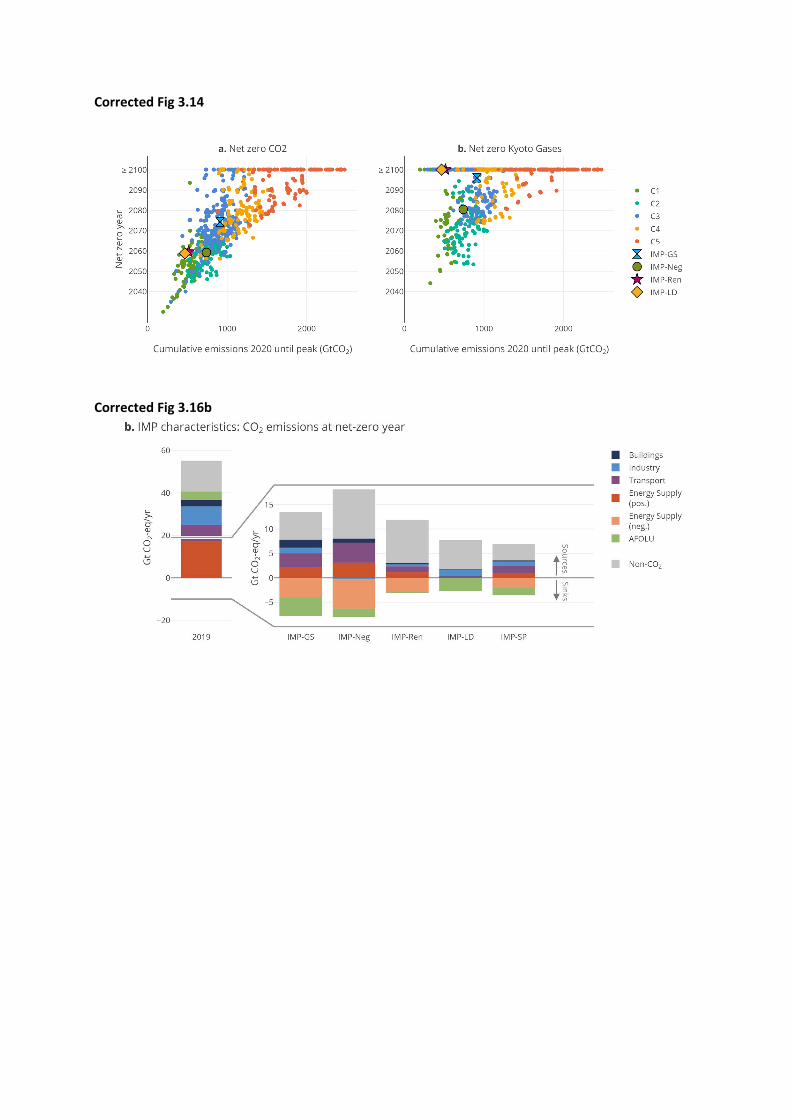
Chapter 3 48 1 Fig 3.16 - updated A new figure to replace existing one
Chapter 3 22 1 Fig 3.6 - updated A new figure to replace existing one
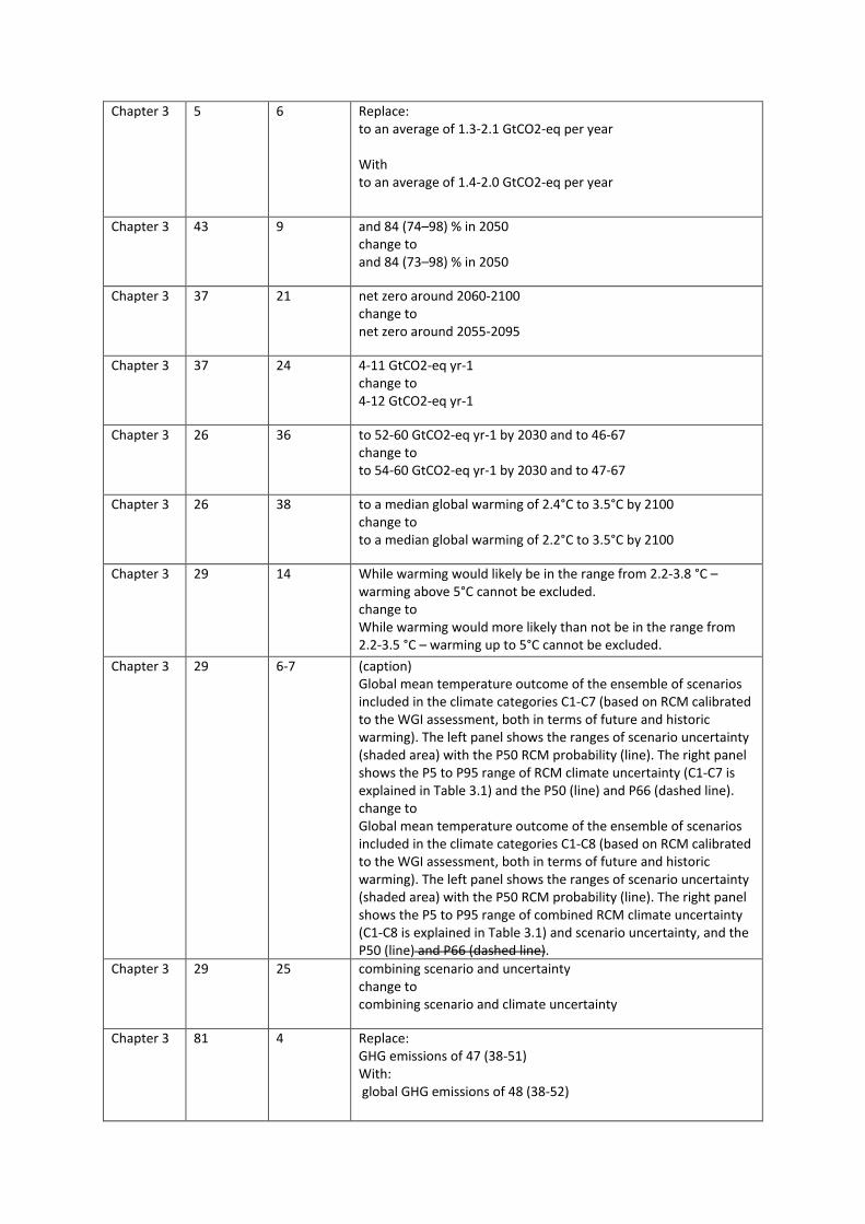
Chapter 3 23 2 Fig 3.7 - updated A new figure to replace existing one
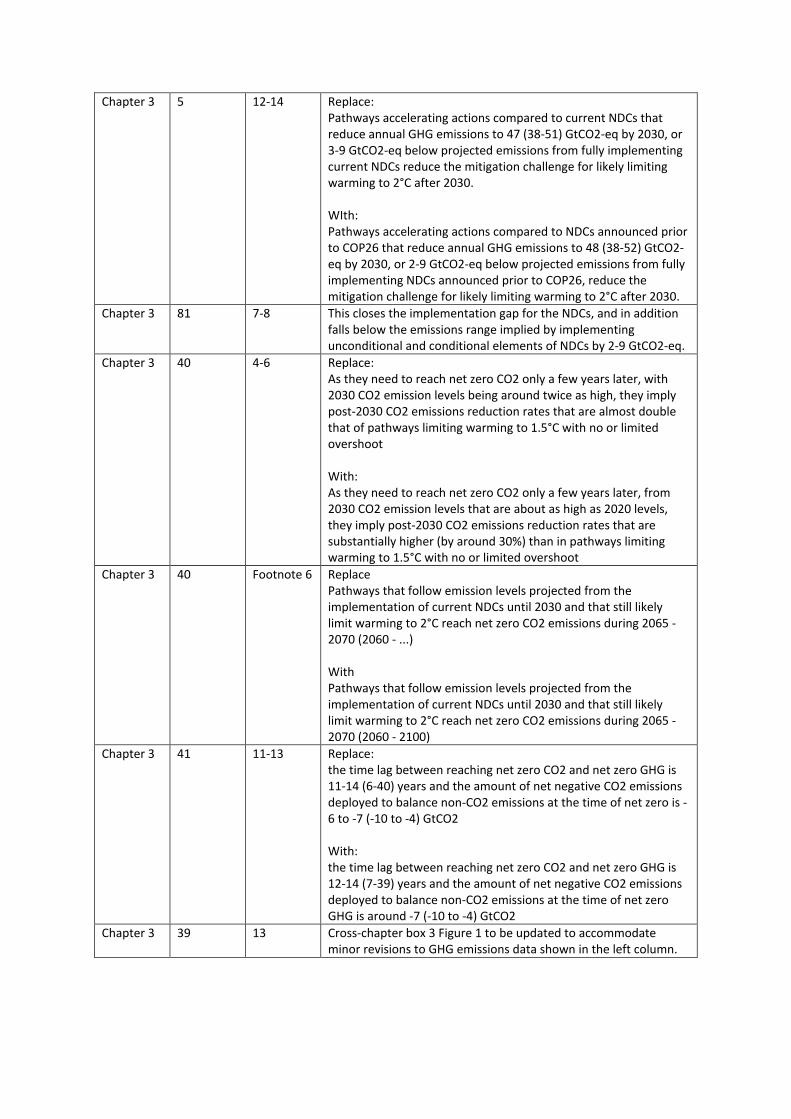
Chapter 3 28 1 Fig 3.10 - updated A new figure to replace existing one
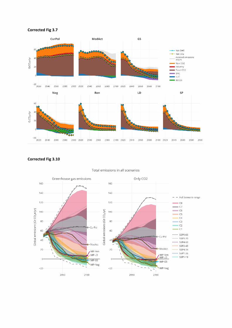
Chapter 3 42 30 Fig 3.14 - updated A new figure to replace existing one
Chapter 3 75 23 Table 3.6 – updated A new figure to replace existing one
Chapter 3 4 16 2.4°C change to: 2.2°C
Chapter 3 4 15 52-60 GtCO2-eq yr-1 by 2030 and to 46-67 change to 54-61 GtCO2-eq yr-1 by 2030 and to 47-67
Chapter 3 73 19-22 Replace with: To still have a likely chance to stay below 2°C, the global post-2030 GHG emission reduction rates would need to be abruptly raised in 2030 from 0-0.7 GtCO2-eq yr-1 to an average of 1.4-2.0 GtCO2-eq yr-1 during the period 2030-2050 (Figure 3.30c), around 70% of that in immediate mitigation pathways confirming findings in the literature (Winning et al. 2019).
Chapter 3 69 1 Replace: reductions would need to abruptly increase after 2030 to an annual average rate of 1.3-2.1 GtCO2-eq during the period 2030-2050, With: reductions would need to abruptly increase after 2030 to an annual average rate of 1.4-2.0 GtCO2-eq during the period 2030-2050,
Chapter 3 72 25-28 Replace: For the 139 scenarios of this kind that are collected in the AR6 scenario database and that still likely limit warming to 2°C, the 2030 emissions range is 52.5 (46.5-56) GtCO2-eq (based on native model reporting) and 52.5 (47-56.5) GtCO2-eq, respectively (based on harmonized emissions data for climate assessment) With: For the 139 scenarios of this kind that are collected in the AR6 scenario database and that still likely limit warming to 2°C, the 2030 emissions range is 53 (45-58) GtCO2-eq (based on native model reporting) and 52.5 (47-56.5) GtCO2-eq, respectively (based on harmonized emissions data for climate assessment)
Chapter 3 72 32-25 Replace: The assessed emission ranges from implementing the unconditional (unconditional and conditional) elements of current NDCs implies an emissions gap to cost-effective mitigation pathways of 20-26 (16-24) GtCO2-eq in 2030 for limiting warming to 1.5°C with no or limited overshoot and 10-17 (7-14) GtCO2-eq in 2030 for likely limiting warming to 2°C With: The assessed emission ranges from implementing the unconditional (unconditional and conditional) elements of current NDCs implies an emissions gap to cost-effective mitigation
pathways of 19-26 (16-23) GtCO2-eq in 2030 for limiting warming to 1.5°C with no or limited overshoot and 10-16 (6-14) GtCO2-eq in 2030 for likely limiting warming to 2°C
Chapter 3 82 1 Figure 3.31 Change title to "GHG emissions"
Chapter 3 75 23 Table 3.6 – Definition of global indicators in the rows need to be clarified: Change in GHG emissions in ... Change in CO2 emissions in ... Change in net land use CO2 emissions in ... Change in CH4 emissons in ... Change in primary energy from coal ... Change in primary energy from oil ... Change in primary energy from gas ... Change in primary energy from nuclear ... Change in primary energy from modern biomass ... Change in primary energy from coal ... Change in carbon intensity of electricity in ... Change in carbon intensity of non-electric final energy consumption in ...
Chapter 3 4 35 with net global GHG emissions of 30-49 GtCO2-eq yr-1 by 2030 and 13-27 GtCO2 change to with net global GHG emissions of 32-55 GtCO2-eq yr-1 by 2030 and 14-26 GtCO2
Chapter 3 4 36-37 This corresponds to reductions, relative to 2019 levels, of 12-46% by 2030 and 52-77% by 2050. change to This corresponds to reductions, relative to 2019 levels, of 13-45% by 2030 and 52-76% by 2050.
Chapter 3 4 40 reductions of 38–63% by 2030 and 75-98% by 2050 relative to 2019 levels. change to reductions of 34–60% by 2030 and 73-98% by 2050 relative to 2019 levels.
Chapter 3 5 32 890 (640-1160) GtCO2 in pathways likely limiting warming to 2.0°C. change to 880 (640-1130) GtCO2 in pathways likely limiting warming to 2.0°C.
Chapter 3 5 37 4-11 GtCO2-eq yr-1 change to 8 (4-12)
Chapter 3 5 6 Replace: to an average of 1.3-2.1 GtCO2-eq per year With to an average of 1.4-2.0 GtCO2-eq per year
Chapter 3 43 9 and 84 (74–98) % in 2050 change to and 84 (73–98) % in 2050
Chapter 3 37 21 net zero around 2060-2100 change to net zero around 2055-2095
Chapter 3 37 24 4-11 GtCO2-eq yr-1 change to 4-12 GtCO2-eq yr-1
Chapter 3 26 36 to 52-60 GtCO2-eq yr-1 by 2030 and to 46-67 change to to 54-60 GtCO2-eq yr-1 by 2030 and to 47-67
Chapter 3 26 38 to a median global warming of 2.4°C to 3.5°C by 2100 change to to a median global warming of 2.2°C to 3.5°C by 2100
Chapter 3 29 14 While warming would likely be in the range from 2.2-3.8 °C – warming above 5°C cannot be excluded. change to While warming would more likely than not be in the range from 2.2-3.5 °C – warming up to 5°C cannot be excluded.
Chapter 3 29 6-7 (caption) Global mean temperature outcome of the ensemble of scenarios included in the climate categories C1-C7 (based on RCM calibrated to the WGI assessment, both in terms of future and historic warming). The left panel shows the ranges of scenario uncertainty (shaded area) with the P50 RCM probability (line). The right panel shows the P5 to P95 range of RCM climate uncertainty (C1-C7 is explained in Table 3.1) and the P50 (line) and P66 (dashed line). change to Global mean temperature outcome of the ensemble of scenarios included in the climate categories C1-C8 (based on RCM calibrated to the WGI assessment, both in terms of future and historic warming). The left panel shows the ranges of scenario uncertainty (shaded area) with the P50 RCM probability (line). The right panel shows the P5 to P95 range of combined RCM climate uncertainty (C1-C8 is explained in Table 3.1) and scenario uncertainty, and the P50 (line) and P66 (dashed line).
Chapter 3 29 25 combining scenario and uncertainty change to combining scenario and climate uncertainty
Chapter 3 81 4 Replace: GHG emissions of 47 (38-51) With: global GHG emissions of 48 (38-52)
Chapter 3 5 12-14 Replace: Pathways accelerating actions compared to current NDCs that reduce annual GHG emissions to 47 (38-51) GtCO2-eq by 2030, or 3-9 GtCO2-eq below projected emissions from fully implementing current NDCs reduce the mitigation challenge for likely limiting warming to 2°C after 2030. WIth: Pathways accelerating actions compared to NDCs announced prior to COP26 that reduce annual GHG emissions to 48 (38-52) GtCO2-eq by 2030, or 2-9 GtCO2-eq below projected emissions from fully implementing NDCs announced prior to COP26, reduce the mitigation challenge for likely limiting warming to 2°C after 2030.
Chapter 3 81 7-8 This closes the implementation gap for the NDCs, and in addition falls below the emissions range implied by implementing unconditional and conditional elements of NDCs by 2-9 GtCO2-eq.
Chapter 3 40 4-6 Replace: As they need to reach net zero CO2 only a few years later, with 2030 CO2 emission levels being around twice as high, they imply post-2030 CO2 emissions reduction rates that are almost double that of pathways limiting warming to 1.5°C with no or limited overshoot With: As they need to reach net zero CO2 only a few years later, from 2030 CO2 emission levels that are about as high as 2020 levels, they imply post-2030 CO2 emissions reduction rates that are substantially higher (by around 30%) than in pathways limiting warming to 1.5°C with no or limited overshoot
Chapter 3 40 Footnote 6 Replace Pathways that follow emission levels projected from the implementation of current NDCs until 2030 and that still likely limit warming to 2°C reach net zero CO2 emissions during 2065 - 2070 (2060 - ...) With Pathways that follow emission levels projected from the implementation of current NDCs until 2030 and that still likely limit warming to 2°C reach net zero CO2 emissions during 2065 - 2070 (2060 - 2100)
Chapter 3 41 11-13 Replace: the time lag between reaching net zero CO2 and net zero GHG is 11-14 (6-40) years and the amount of net negative CO2 emissions deployed to balance non-CO2 emissions at the time of net zero is -6 to -7 (-10 to -4) GtCO2 With: the time lag between reaching net zero CO2 and net zero GHG is 12-14 (7-39) years and the amount of net negative CO2 emissions deployed to balance non-CO2 emissions at the time of net zero GHG is around -7 (-10 to -4) GtCO2
Chapter 3 39 13 Cross-chapter box 3 Figure 1 to be updated to accommodate minor revisions to GHG emissions data shown in the left column.
Corrected Fig 3.7
Corrected Fig 3.10
Corrected Fig 3.14
Corrected Fig 3.16b

Do Not Cite, Quote or Distribute 3-1 Total pages: 156
Chapter 3: Mitigation Pathways Compatible with Long-Term 1
Goals 2
3
Coordinating Lead Authors: Keywan Riahi (Austria), Roberto Schaeffer (Brazil) 4
5
Lead Authors: Jacobo Arango (Colombia), Katherine Calvin (the United States of America), Céline 6
Guivarch (France), Tomoko Hasegawa, (Japan), Kejun Jiang (China), Elmar Kriegler (Germany), 7
Robert Matthews (United Kingdom), Glen Peters (Norway/Australia), Anand Rao (India), Simon 8
Robertson (Australia), Adam Mohammed Sebbit (Uganda), Julia Steinberger (United 9
Kingdom/Switzerland), Massimo Tavoni (Italy), Detlef van Vuuren (the Netherlands) 10
11
Contributing Authors: Alaa Al Khourdajie (United Kingdom/Syria), Christoph Bertram (Germany), 12
Valentina Bosetti (Italy), Elina Brutschin (Austria), Edward Byers (Austria/Ireland), Tamma Carleton 13
(the United States of America), Leon Clarke (the United States of America), Annette Cowie 14
(Australia), Delavane Diaz (the United States of America), Laurent Drouet (Italy/France), Navroz 15
Dubash (India), Jae Edmonds (the United States of America) Jan S. Fuglestvedt (Norway), Shinichiro 16
Fujimori (Japan), Oliver Geden (Germany), Giacomo Grassi (Italy/European Union), Michael Grubb 17
(United Kingdom), Anders Hammer Strømman (Norway), Frank Jotzo (Australia), Jarmo Kikstra 18
(Austria/the Netherlands), Zbigniew Klimont (Austria/Poland), Alexandre Köberle (Brazil/United 19
Kingdom), Robin Lamboll (United Kingdom/the United States of America), Franck Lecocq (France), 20
Jared Lewis (Australia/New Zealand), Yun Seng Lim (Malaysia), Giacomo Marangoni (Italy), Eric 21
Masanet (the United States of America), Toshihiko Masui (Japan), David McCollum (the United 22
States of America), Malte Meinshausen (Australia/Germany), Aurélie Méjean (France), Joel 23
Millward-Hopkins (United Kingdom), Catherine Mitchell (United Kingdom), Gert-Jan Nabuurs (the 24
Netherlands), Zebedee Nicholls (Australia), Brian O’Neill (the United States of America), Anthony 25
Patt (the United States of America/Switzerland), Franziska Piontek (Germany), Andy Reisinger (New 26
Zealand), Joeri Rogelj (United Kingdom/Belgium), Steven Rose (the United States of America), 27
Bastiaan van Ruijven (Austria/the Netherlands), Yamina Saheb (France/Switzerland/Algeria), Marit 28
Sandstad (Norway), Jim Skea (United Kingdom), Chris Smith (Austria/United Kingdom), Björn 29
Soergel (Germany), Florian Tirana (France), Kaj-Ivar van der Wijst (the Netherlands), Harald 30
Winkler (South Africa) 31
32
Review Editors: Vaibhav Chaturvedi (India), Wenying Chen (China), Julio Torres Martinez (Cuba) 33
34
Chapter Scientists: Edward Byers (Austria/Ireland), Eduardo Müller-Casseres (Brazil) 35
36
Date of Draft: 27/11/202137 ACCEPTED VERSIO
N
SUBJECT TO FIN
AL EDITS
Final Government Distribution Chapter 3 IPCC AR6 WGIII
Do Not Cite, Quote or Distribute 3-2 Total pages: 156
Table of Contents 1
2 Chapter 3: Mitigation Pathways Compatible with Long-Term Goals ........................................... 3-1 3
Executive summary .......................................................................................................................... 3-4 4
3.1 Introduction ........................................................................................................................ 3-10 5
3.1.1 Assessment of mitigation pathways and their compatibility with long-term goals ... 3-10 6
3.1.2 Linkages to other Chapters in the Report ................................................................... 3-10 7
3.1.3 Complementary use of large scenario ensembles and a limited set of Illustrative 8
Mitigation Pathways (IMPs) ...................................................................................................... 3-11 9
3.2 What are mitigation pathways compatible with long-term goals? ..................................... 3-12 10
3.2.1 Scenarios and emission pathways .............................................................................. 3-12 11
3.2.2 The utility of Integrated Assessment Models ............................................................. 3-13 12
3.2.3 The scenario literature and scenario databases .......................................................... 3-15 13
3.2.4 The AR6 scenario database ........................................................................................ 3-16 14
3.2.5 Illustrative Mitigation Pathways ................................................................................ 3-19 15
3.3 Emission pathways, including socio-economic, carbon budget and climate responses 16
uncertainties ................................................................................................................................... 3-24 17
3.3.1 Socio-economic drivers of emissions scenarios ......................................................... 3-24 18
3.3.2 Emission pathways and temperature outcomes .......................................................... 3-26 19
Cross-Chapter Box 3: Understanding net zero CO2 and net zero GHG emissions .................... 3-37 20
3.3.3 Climate impacts on mitigation potential .................................................................... 3-49 21
3.4 Integrating sectoral analysis into systems transformations ................................................ 3-50 22
3.4.1 Cross-sector linkages ................................................................................................. 3-51 23
3.4.2 Energy supply ............................................................................................................ 3-57 24
3.4.3 Buildings .................................................................................................................... 3-59 25
3.4.4 Transport .................................................................................................................... 3-61 26
3.4.5 Industry ...................................................................................................................... 3-63 27
3.4.6 Agriculture, Forestry and Other Land Use (AFOLU) ................................................ 3-64 28
3.4.7 Other Carbon Dioxide Removal Options ................................................................... 3-67 29
3.5 Interaction between near-, medium- and long-term action in mitigation pathways ........... 3-68 30
3.5.1 Relationship between long-term climate goals and near- to medium-term emissions 31
reductions ................................................................................................................................... 3-69 32
3.5.2 Implications of near-term emission levels for keeping long-term climate goals within 33
reach 3-72 34
3.6 Economics of long-term mitigation and development pathways, including mitigation costs 35
and benefits .................................................................................................................................... 3-82 36
3.6.1 Economy-wide implications of mitigation ................................................................. 3-83 37
3.6.2 Economic benefits of avoiding climate changes impacts........................................... 3-91 38
3.6.3 Aggregate economic implication of mitigation co-benefits and trade-offs ................ 3-95 39
3.6.4 Structural change, employment and distributional issues along mitigation pathways ... 3-40
95 41
ACCEPTED VERSION
SUBJECT TO FIN
AL EDITS
Final Government Distribution Chapter 3 IPCC AR6 WGIII
Do Not Cite, Quote or Distribute 3-3 Total pages: 156
3.7 Sustainable development, mitigation and avoided impacts ............................................... 3-97 1
3.7.1 Synthesis findings on mitigation and sustainable development ................................. 3-97 2
3.7.2 Food ......................................................................................................................... 3-102 3
3.7.3 Water ........................................................................................................................ 3-103 4
3.7.4 Energy ...................................................................................................................... 3-104 5
3.7.5 Health ....................................................................................................................... 3-105 6
3.7.6 Biodiversity (land and water) ................................................................................... 3-107 7
3.7.7 Cities and infrastructure ........................................................................................... 3-108 8
3.8 Feasibility of socio/techno/economic transitions ............................................................. 3-109 9
3.8.1 Feasibility frameworks for the low carbon transition and scenarios ........................ 3-109 10
3.8.2 Feasibility appraisal of low carbon scenarios .......................................................... 3-110 11
3.8.3 Feasibility in the light of socio-technical transitions ............................................... 3-114 12
3.8.4 Enabling factors ....................................................................................................... 3-115 13
3.9 Methods of assessment and gaps in knowledge and data ................................................ 3-116 14
3.9.1 AR6 mitigation pathways ......................................................................................... 3-116 15
3.9.2 Models assessed in this chapter ............................................................................... 3-116 16
Frequently Asked Questions (FAQs) ........................................................................................... 3-117 17
References .................................................................................................................................... 3-119 18
19
20
21
ACCEPTED VERSION
SUBJECT TO FIN
AL EDITS
Final Government Distribution Chapter 3 IPCC AR6 WGIII
Do Not Cite, Quote or Distribute 3-4 Total pages: 156
Executive summary 1
Chapter 3 assesses the emissions pathways literature in order to identify their key 2
characteristics (both in commonalities and differences) and to understand how societal choices 3
may steer the system into a particular direction (high confidence). More than 2000 quantitative 4
emissions pathways were submitted to the IPCC’s Sixth Assessment Report (AR6) database, out of 5
which 1202 scenarios included sufficient information for assessing the associated warming consistent 6
with WGI. Five Illustrative Mitigation Pathways (IMPs) were selected, each emphasizing a different 7
scenario element as its defining feature: heavy reliance on renewables (IMP-Ren), strong emphasis on 8
energy demand reductions (IMP-LD), extensive use of CDR in the energy and the industry sectors to 9
achieve net negative emissions (IMP-Neg), mitigation in the context of broader sustainable 10
development (IMP-SP), and the implications of a less rapid and gradual strengthening of near-term 11
mitigation actions (IMP-GS).{3.2, 3.3} 12
13
Pathways consistent with the implementation and extrapolation of countries’ current policies 14
see GHG emissions reaching 52-60 GtCO2-eq yr-1 by 2030 and to 46-67 GtCO2-eq yr-1 by 2050, 15
leading to a median global warming of 2.4°C to 3.5°C by 2100 (medium confidence). These 16
pathways consider policies at the time that they were developed. The Shared Socioeconomic 17
Pathways (SSPs) permit a more systematic assessment of future GHG emissions and their 18
uncertainties than was possible in AR5. The main emissions drivers include growth in population, 19
reaching 8.5-9.7 billion by 2050, and an increase in global GDP of 2.7-4.1% per year between 2015 20
and 2050. Final energy demand in the absence of any new climate policies is projected to grow to 21
around 480 to 750 EJ yr-1 in 2050 (compared to around 390 EJ in 2015). (medium confidence) The 22
highest emissions scenarios in the literature result in global warming of >5°C by 2100, based on 23
assumptions of rapid economic growth and pervasive climate policy failures. (high confidence). {3.3} 24
25
Many pathways in the literature show how to likely limit global warming compared to 26
preindustrial times to 2°C with no overshoot or to 1.5°C with limited overshoot. The likelihood 27
of limiting warming to 1.5C with no or limited overshoot has dropped in AR6 compared to 28
SR1.5 because global GHG emissions have risen since the time SR1.5 was published, leading to 29
higher near-term emissions (2030) and higher cumulative CO2 emissions until the time of net 30
zero (medium confidence). Only a small number of published pathways limit global warming to 31
1.5°C without overshoot over the course of the 21st century. {3.3, Annex III.II.3} 32
33
Cost-effective mitigation pathways assuming immediate actions to likely limit warming to 2°C 34
are associated with net global GHG emissions of 30-49 GtCO2-eq yr-1 by 2030 and 13-27 GtCO2-35
eq yr-1 by 2050 (medium confidence). This corresponds to reductions, relative to 2019 levels, of 12-36
46% by 2030 and 52-77% by 2050. Pathways that limit global warming to below 1.5°C with no or 37
limited overshoot require a further acceleration in the pace of the transformation, with net GHG 38
emissions typically around 21-36 GtCO2-eq yr-1 by 2030 and 1-15 GtCO2-eq yr-1 by 2050; thus 39
reductions of 38–63% by 2030 and 75-98% by 2050 relative to 2019 levels. {3.3} 40
Pathways following current NDCs1 until 2030 reach annual emissions of 47-57 GtCO2-eq by 41
2030, thereby making it impossible to limit warming to 1.5°C with no or limited overshoot and 42
strongly increasing the challenge to likely limit warming to 2°C (high confidence). A high 43
FOOTNOTE 1 Current NDCs refers to the most recent nationally determined contributions submitted to the
UNFCCC as well as those publicly announced with sufficient detail on targets, but not yet submitted, up to 11
October 2021, and reflected in studies published up to 11 October 2021.
ACCEPTED VERSION
SUBJECT TO FIN
AL EDITS
Final Government Distribution Chapter 3 IPCC AR6 WGIII
Do Not Cite, Quote or Distribute 3-5 Total pages: 156
overshoot of 1.5°C increases the risks from climate impacts and increases the dependence on large 1
scale carbon dioxide removal from the atmosphere. A future consistent with current NDCs implies 2
higher fossil fuel deployment and lower reliance on low carbon alternatives until 2030, compared to 3
mitigation pathways with immediate action to likely limit warming to 2°C and below. To likely limit 4
warming to 2°C after following the NDCs to 2030, the pace of global GHG emission reductions 5
would need to accelerate quite rapidly from 2030 onward: to an average of 1.3-2.1 GtCO2-eq per year 6
between 2030 and 2050, which is similar to global CO2 emission reductions in 2020 due to the 7
COVID-19 pandemic, and around 70% faster than in immediate action pathways likely limiting 8
warming to 2°C. Accelerating emission reductions after following an NDC pathway to 2030 would be 9
particularly challenging because of the continued build-up of fossil fuel infrastructure that would be 10
expected to take place between now and 2030. {3.5, 4.2} 11
Pathways accelerating actions compared to current NDCs that reduce annual GHG emissions to 12
47 (38-51) GtCO2-eq by 2030, or 3-9 GtCO2-eq below projected emissions from fully 13
implementing current NDCs reduce the mitigation challenge for likely limiting warming to 2°C 14
after 2030. (medium confidence). The accelerated action pathways are characterized by a global, but 15
regionally differentiated, roll-out of regulatory and pricing policies. Compared to NDCs, they see less 16
fossil fuels and more low-carbon fuels until 2030, and narrow, but do not close the gap to pathways 17
assuming immediate global action using all available least-cost abatement options. All delayed or 18
accelerated action pathways likely limiting warming to below 2°C converge to a global mitigation 19
regime at some point after 2030 by putting a significant value on reducing carbon and other GHG 20
emissions in all sectors and regions. {3.5} 21
Mitigation pathways limiting warming to 1.5°C with no or limited overshoot reach 50% 22
reductions of CO2 in the 2030s, relative to 2019, then reduce emissions further to reach net zero 23
CO2 emissions in the 2050s. Pathways likely limiting warming to 2°C reach 50% reductions in 24
the 2040s and net zero CO2 by 2070s (medium confidence). {3.3, Cross-Chapter Box 3 in Chapter 25
3} 26
27
Peak warming in mitigation pathways is determined by the cumulative net CO2 emissions until 28
the time of net zero CO2 and the warming contribution of other GHGs and climate forcers at 29
that time (high confidence). Cumulative net CO2 emissions from 2020 to the time of net zero CO2 30
are 510 (330-710) GtCO2 in pathways that limit warming to 1.5°C with no or limited overshoot and 31
890 (640-1160) GtCO2 in pathways likely limiting warming to 2.0°C. These estimates are consistent 32
with the assessment of remaining carbon budgets by WGI after adjusting for differences in peak 33
warming levels. {3.3, Box 3.4} 34
Rapid reductions in non-CO2 GHGs, particularly methane, would lower the level of peak 35
warming (high confidence). Residual non-CO2 emissions at the time of reaching net zero CO2 range 36
between 4-11 GtCO2-eq yr-1 in pathways likely limiting warming to 2.0°C or below. Methane (CH4) 37
is reduced by around 20% (1-46%) in 2030 and almost 50% (26-64%) in 2050, relative to 2019. 38
Methane emission reductions in pathways limiting warming to 1.5°C with no or limited overshoot are 39
substantially higher by 2030, 33% (19-57%), but only moderately so by 2050, 50% (33-69%). 40
Methane emissions reductions are thus attainable at relatively lower GHG prices but are at the same 41
time limited in scope in most 1.5-2°C pathways. Deeper methane emissions reductions by 2050 could 42
further constrain the peak warming. N2O emissions are reduced too, but similar to CH4, emission 43
reductions saturate for more stringent climate goals. In the mitigation pathways, the emissions of 44
cooling aerosols are reduced due to reduced use of fossil fuels. The overall impact on non-CO2-related 45
warming combines these factors. {3.3} 46
ACCEPTED VERSION
SUBJECT TO FIN
AL EDITS
Final Government Distribution Chapter 3 IPCC AR6 WGIII
Do Not Cite, Quote or Distribute 3-6 Total pages: 156
Net zero GHG emissions imply net negative CO2 emissions at a level compensating residual non-1
CO2 emissions. Only 30% of the pathways likely limiting warming to 2°C or below reach net 2
zero GHG emissions in the 21st century. (high confidence). In those pathways reaching net zero 3
GHGs, it is achieved around 10-20 years later than for net zero CO2. (medium confidence). The 4
reported quantity of residual non-CO2 emissions depends on accounting: the choice of GHG metric. 5
Reaching and sustaining global net zero GHG emissions, measured in terms of GWP-100, results in a 6
gradual decline of temperature. (high confidence) {3.3, Cross-Chapter Box 3 in Chapter 3, Cross-7
Chapter Box 2 in Chapter 2} 8
9
Pathways likely limiting warming to 2°C and below exhibit substantial reductions in emissions 10
from all sectors (high confidence). Projected CO2 emissions reductions between 2019 and 2050 in 11
1.5°C pathways with no or limited overshoot are around 77% (31-96%) for energy demand, 115% for 12
energy supply (90 to 167%), and 148% for AFOLU (94 to 387%). In pathways likely limiting 13
warming to 2°C, projected CO2 emissions are reduced between 2019 and 2050 by around 49% for 14
energy demand, 97% for energy supply, and 136% for AFOLU. (medium confidence){3.4} 15
16
Delaying or sacrificing emissions reductions in one sector or region involves compensating 17
reductions in other sectors or regions if warming is to be limited (high confidence). Mitigation 18
pathways show differences in the timing of decarbonization and when net zero CO2 emissions are 19
achieved across sectors and regions. At the time of global net zero CO2 emissions, emissions in some 20
sectors and regions are positive while others are negative; the ordering depends on the mitigation 21
options available, the cost of those options, and the policies implemented. In cost-effective mitigation 22
pathways, the energy supply sector typically reaches net zero CO2 before the economy as a whole, 23
while the demand sectors reach net zero CO2 later, if ever (high confidence). {3.4} 24
25
Pathways likely limiting warming to 2°C and below involve substantial reductions in fossil fuel 26
consumption and a near elimination of the use of coal without CCS (high confidence). These 27
pathways show an increase in low carbon energy, with 88% (69-97%) of primary energy coming from 28
these sources by 2100. {3.4} 29
30
Stringent emissions reductions at the level required for 2°C and below are achieved through 31
increased direct electrification of buildings, transport, and industry, resulting in increased 32
electricity generation in all pathways (high confidence). Nearly all electricity in pathways likely 33
limiting warming to 2℃ or below is from low or no carbon technologies, with different shares of 34
nuclear, biomass, non-biomass renewables, and fossil CCS across pathways. {3.4} 35
36
The measures required to likely limit warming to 2°C or below can result in large scale 37
transformation of the land surface (high confidence). Pathways likely limiting warming to 2°C or 38
below are projected to reach net zero CO2 emissions in the AFOLU sector between 2020s and 2070, 39
with an increase of forest cover of about 322 million ha (-67 to 890 million ha) in 2050 in pathways 40
limiting warming to 1.5°C with no or limited overshoot. Cropland area to supply biomass for 41
bioenergy (including BECCS) is around 199 (56-482) million ha in 2100 in pathways limiting 42
warming to 1.5°C with no or limited overshoot. The use of bioenergy can lead to either increased or 43
reduced emissions, depending on the scale of deployment, conversion technology, fuel displaced, and 44
how/where the biomass is produced (high confidence). {3.4} 45
46
Anthropogenic land CO2 emissions and removals in IAM pathways cannot be directly compared 47
with those reported in national GHG inventories (high confidence). Methodologies enabling a 48
more like-for-like comparison between models’ and countries’ approaches would support more 49
accurate assessment of the collective progress achieved under the Paris Agreement. {3.4, 7.2.2.5} 50
ACCEPTED VERSION
SUBJECT TO FIN
AL EDITS

Final Government Distribution Chapter 3 IPCC AR6 WGIII
Do Not Cite, Quote or Distribute 3-7 Total pages: 156
1
Pathways that likely limiting warming to 2°C or below involve some amount of CDR to 2
compensate for residual GHG emissions remaining after substantial direct emissions reductions 3
in all sectors and regions (high confidence). CDR deployment in pathways serves multiple 4
purposes: accelerating the pace of emissions reductions, offsetting residual emissions, and creating the 5
option for net negative CO2 emissions in case temperature reductions need to be achieved in the long 6
term (high confidence). CDR options in the pathways are mostly limited to BECCS, afforestation and 7
DACCS. CDR through some measures in AFOLU can be maintained for decades but not in the very 8
long term because these sinks will ultimately saturate (high confidence). {3.4} 9
10
Mitigation pathways show reductions in energy demand relative to reference scenarios, through 11
a diverse set of demand-side interventions (high confidence). Bottom-up and non-IAM studies 12
show significant potential for demand-side mitigation. A stronger emphasis on demand-side 13
mitigation implies less dependence on CDR and, consequently, reduced pressure on land and 14
biodiversity. {3.4, 3.7} 15
16
Limiting warming requires shifting energy investments away from fossil-fuels and towards low-17
carbon technologies (high confidence). The bulk of investments are needed in medium- and low-18
income regions. Investment needs in the electricity sector are on average 2.3 trillion USD2015 yr-1 19
over 2023-2052 for pathways limiting temperature to 1.5°C with no or limited overshoot, and 1.7 20
trillion USD2015 yr-1 for pathways likely limiting warming to 2°C. {3.6.1} 21
22
Pathways likely avoiding overshoot of 2°C warming require more rapid near-term 23
transformations and are associated with higher up-front transition costs, but meanwhile bring 24
long-term gains for the economy as well as earlier benefits in avoided climate change impacts 25
(high confidence). This conclusion is independent of the discount rate applied, though the modelled 26
cost-optimal balance of mitigation action over time does depend on the discount rate. Lower discount 27
rates favour earlier mitigation, reducing reliance on CDR and temperature overshoot. {3.6.1, 3.8} 28
29
Mitigation pathways likely limiting warming to 2°C entail losses in global GDP with respect to 30
reference scenarios of between 1.3% and 2.7% in 2050; and in pathways limiting warming to 31
1.5°C with no or limited overshoot, losses are between 2.6% and 4.2%. Yet, these estimates do 32
not account for the economic benefits of avoided climate change impacts (medium confidence). 33
In mitigation pathways likely limiting warming to 2°C, marginal abatement costs of carbon are about 34
90 (60-120) USD2015/tCO2 in 2030 and about 210 (140-340) USD2015/tCO2 in 2050; in pathways 35
that limit warming to 1.5°C with no or limited overshoot, they are about 220 (170-290) 36
USD2015/tCO2 in 2030 and about 630 (430-990) USD2015/tCO2 in 20502. {3.6.1} 37
38
The global benefits of pathways likely limiting warming to 2°C outweigh global mitigation costs 39
over the 21st century, if aggregated economic impacts of climate change are at the moderate to 40
high end of the assessed range, and a weight consistent with economic theory is given to 41
economic impacts over the long-term. This holds true even without accounting for benefits in 42
other sustainable development dimensions or non-market damages from climate change 43
(medium confidence). The aggregate global economic repercussions of mitigation pathways include 44
the macroeconomic impacts of investments in low-carbon solutions and structural changes away from 45
emitting activities, co-benefits and adverse side effects of mitigation, (avoided) climate change 46
impacts, and (reduced) adaptation costs. Existing quantifications of global aggregate economic 47
FOOTNOTE2 Numbers in parenthesis represent he interquartile range of the scenario samples.
ACCEPTED VERSION
SUBJECT TO FIN
AL EDITS
Final Government Distribution Chapter 3 IPCC AR6 WGIII
Do Not Cite, Quote or Distribute 3-8 Total pages: 156
impacts show a strong dependence on socioeconomic development conditions, as these shape 1
exposure and vulnerability and adaptation opportunities and responses. (Avoided) impacts for poorer 2
households and poorer countries represent a smaller share in aggregate economic quantifications 3
expressed in GDP or monetary terms, whereas their well-being and welfare effects are comparatively 4
larger. When aggregate economic benefits from avoided climate change impacts are accounted for, 5
mitigation is a welfare-enhancing strategy. (high confidence) {3.6.2} 6
7
The economic benefits on human health from air quality improvement arising from mitigation 8
action can be of the same order of magnitude as mitigation costs, and potentially even larger 9
(medium confidence). {3.6.3} 10
11
Differences between aggregate employment in mitigation pathways compared to reference 12
scenarios are relatively small, although there may be substantial reallocations across sectors, 13
with job creation in some sectors and job losses in others. The net employment effect (and its sign) 14
depends on scenario assumptions, modelling framework, and modelled policy design. Mitigation has 15
implications for employment through multiple channels, each of which impacts geographies, sectors 16
and skill categories differently. (medium confidence) {3.6.4} 17
18
The economic repercussions of mitigation vary widely across regions and households, depending 19
on policy design and level of international cooperation (high confidence). Delayed global 20
cooperation increases policy costs across regions, especially in those that are relatively carbon 21
intensive at present (high confidence). Pathways with uniform carbon values show higher mitigation 22
costs in more carbon-intensive regions, in fossil-fuels exporting regions and in poorer regions (high 23
confidence). Aggregate quantifications expressed in GDP or monetary terms undervalue the economic 24
effects on households in poorer countries; the actual effects on welfare and well-being are 25
comparatively larger (high confidence). Mitigation at the speed and scale required to likely limit 26
warming to 2°C or below implies deep economic and structural changes, thereby raising multiple 27
types of distributional concerns across regions, income classes and sectors (high confidence). {3.6.1, 28
3.6.4} 29
30
The timing of mitigation actions and their effectiveness will have significant consequences for 31
broader sustainable development outcomes in the longer term (high confidence). Ambitious 32
mitigation can be considered a precondition for achieving the Sustainable Development Goals, 33
especially for vulnerable populations and ecosystems with little capacity to adapt to climate impacts. 34
Dimensions with anticipated co-benefits include health, especially regarding air pollution, clean 35
energy access and water availability. Dimensions with potential trade-offs include food, employment, 36
water stress, and biodiversity, which come under pressure from large-scale CDR deployment, energy 37
affordability/access, and mineral resource extraction. (high confidence) {3.7} 38
39
Many of the potential trade-offs of mitigation measures for other sustainable development 40
outcomes depend on policy design and can thus be compensated or avoided with additional 41
policies and investments or through policies that integrate mitigation with other SDGs (high 42
confidence). Targeted SDG policies and investments, for example in the areas of healthy nutrition, 43
sustainable consumption and production, and international collaboration, can support climate change 44
mitigation policies and resolve or alleviate trade-offs. Trade-offs can be addressed by complementary 45
policies and investments, as well as through the design of cross-sectoral policies integrating 46
mitigation with the Sustainable Development Goals of health, nutrition, sustainable consumption and 47
production, equity and biodiversity. {3.7} 48
49
ACCEPTED VERSION
SUBJECT TO FIN
AL EDITS
Final Government Distribution Chapter 3 IPCC AR6 WGIII
Do Not Cite, Quote or Distribute 3-9 Total pages: 156
Decent living standards, which encompass many SDG dimensions, are achievable at lower 1
energy use than previously thought (high confidence). Mitigation strategies that focus on lower 2
demands for energy and land-based resources exhibit reduced trade-offs and negative consequences 3
for sustainable development relative to pathways involving either high emissions and climate impacts 4
or those with high consumption and emissions that are ultimately compensated by large quantities of 5
BECCS. {3.7} 6
7
Different mitigation pathways are associated with different feasibility challenges, though 8
appropriate enabling conditions can reduce these challenges. Feasibility challenges are transient 9
and concentrated in the next two to three decades (high confidence). They are multi-dimensional, 10
context-dependent and malleable to policy, technological and societal trends. {3.8} 11
12
Mitigation pathways are associated with significant institutional and economic feasibility 13
challenges rather than technological and geophysical. The rapid pace of technological 14
development and deployment in mitigation pathways is not incompatible with historical records. 15
Institutional capacity is rather a key limiting factor for a successful transition. Emerging economies 16
appear to have highest feasibility challenges in the short to medium term. {3.8} 17
18
Pathways relying on a broad portfolio of mitigation strategies are more robust and resilient 19
(high confidence). Portfolios of technological solutions reduce the feasibility risks associated with the 20
low carbon transition. {3.8} 21
22
23
ACCEPTED VERSION
SUBJECT TO FIN
AL EDITS
Final Government Distribution Chapter 3 IPCC AR6 WGIII
Do Not Cite, Quote or Distribute 3-10 Total pages: 156
1
3.1 Introduction 2
3.1.1 Assessment of mitigation pathways and their compatibility with long-term goals 3
Chapter 3 takes a long-term perspective on climate change mitigation pathways. Its focus is on the 4
implications of long-term targets for the required short- and medium-term system changes and 5
associated greenhouse gas (GHG) emissions. This focus dictates a more global view and on issues 6
related to path-dependency and up-scaling of mitigation options necessary to achieve different 7
emissions trajectories, including particularly deep mitigation pathways that require rapid and 8
fundamental changes. 9
10
Stabilizing global average temperature change requires to reduce CO2 emissions to net zero. Thus, a 11
central cross-cutting topic within the Chapter is the timing of reaching net zero CO2 emissions and 12
how a “balance between anthropogenic emissions by sources and removals by sinks” could be 13
achieved across time and space. This includes particularly the increasing body of literature since the 14
IPCC Special Report on Global Warming of 1.5C (SR1.5) which focuses on net zero CO2 emissions 15
pathways that avoid temperature overshoot and hence do not rely on net negative CO2 emissions. The 16
chapter conducts a systematic assessment of the associated economic costs as well as the benefits of 17
mitigation for other societal objectives, such as the Sustainable Development Goals (SDGs). In 18
addition, the Chapter builds on SR1.5 and introduces a new conceptual framing for the assessment of 19
possible social, economic, technical, political, and geophysical “feasibility” concerns of alternative 20
pathways, including the enabling conditions that would need to fall into place so that stringent climate 21
goals become attainable. 22
23
The structure of the Chapter is as follows: Section 3.2 introduces different types of mitigation 24
pathways as well as the available modelling. Section 3.3 explores different emissions trajectories 25
given socio-economic uncertainties and consistent with different long-term climate outcomes. A 26
central element in this section is the systematic categorization of the scenario space according to key 27
characteristics of the mitigation pathways (including e.g., global average temperature change, socio-28
economic development, technology assumptions, etc.). In addition, the section introduces selected 29
Illustrative Mitigation Pathways (IMPs) that are used across the whole report. Section 3.4 conducts a 30
sectoral analysis of the mitigation pathways, assessing the pace and direction of systems changes 31
across sectors. Among others, this section aims at the integration of the sectoral information across 32
WGIII AR6 chapters through a comparative assessment of the sectoral dynamics in economy-wide 33
systems models compared to the insights from bottom-up sectoral models (from Chapters 6-11). 34
Section 3.5 focuses on the required timing of mitigation actions, and implication of near-term choices 35
for the attainability of a range of long-term climate goals. After having explored the underlying 36
systems transitions and the required timing of the mitigation actions, Section 3.6 assesses the 37
economic implications, mitigation costs and benefits; and Section 3.7 assesses related co-benefits, 38
synergies, and possible trade-offs for sustainable development and other societal (non-climate) 39
objectives. Section 3.8 assumes a central role in the Chapter and introduces a multi-dimensional 40
feasibility metric that permits the evaluation of mitigation pathways across a range of feasibility 41
concerns. Finally, methods of the assessment and knowledge gaps are discussed in Section 3.9, 42
followed by Frequently Asked Questions. 43
44
3.1.2 Linkages to other Chapters in the Report 45
Chapter 3 is linked to many other chapters in the report. The most important connections exist with 46
Chapter 4 on mitigation and development pathways in the near to mid-term, with the sectoral chapters 47
(Chapters 6-11), with the chapters dealing with cross-cutting issues (e.g., feasibility), and finally also 48
with WGI and WGII AR6. 49
ACCEPTED VERSION
SUBJECT TO FIN
AL EDITS
Final Government Distribution Chapter 3 IPCC AR6 WGIII
Do Not Cite, Quote or Distribute 3-11 Total pages: 156
1
Within the overall framing of the AR6 report, Chapter 3 and Chapter 4 provide important 2
complementary views of the required systems transitions across different temporal and spatial scales. 3
While Chapter 3 focuses on the questions concerning the implications of the long-term objectives for 4
the medium-to-near-term transformations, Chapter 4 comes from the other direction, and focuses on 5
current near-term trends and policies (such as the Nationally Determined Contributions - NDCs) and 6
their consequences with regards to GHG emissions. The latter chapter naturally focuses thus much 7
more on the regional and national dimensions, and the heterogeneity of current and planned policies. 8
Bringing together the information from these two chapters enables the assessment of whether current 9
and planned actions are consistent with the required systems changes for the long-term objectives of 10
the Paris Agreement. 11
12
Important other linkages comprise the collaboration with the “sectoral” Chapters 6-11 to provide an 13
integrated cross-sectoral perspective. This information (including information also from the sectoral 14
chapters) is taken up ultimately also by Chapter 5 on demand/services and Chapter 12 for a further 15
assessment of sectoral potential and costs. 16
17
Linkages to other chapters exist also on the topic of feasibility, which are informed by the policy, the 18
sectoral and the demand chapters, the technology and finance chapters, as well as Chapter 4 on 19
national circumstances. 20
21
Close collaboration with WGI permitted the use of AR6-calibrated emulators, which assure full 22
consistency across the different working groups. Linkages to WGII concern the assessment of macro-23
economic benefits of avoided impacts that are put into the context of mitigation costs as well as co-24
benefits and trade-offs for sustainable development. 25
26
3.1.3 Complementary use of large scenario ensembles and a limited set of Illustrative 27
Mitigation Pathways (IMPs) 28
The assessment of mitigation pathways explores a wide scenario space from the literature within 29
which seven Illustrative Pathways (IPs) are explored. The overall process is indicated in Figure 3.5a. 30
31
For a comprehensive assessment, a large ensemble of scenarios is collected and made available 32
through an interactive AR6 scenario database. The collected information is shared across the chapters 33
of AR6 and includes more than 3000 different pathways from a diverse set of studies. After an initial 34
screening and quality control, scenarios were further vetted to assess if they sufficiently represented 35
historical trends (Annex III). Subsequently, the climate consequences of each scenario were assessed 36
using the climate emulator (leading to further classification). The assessment in Chapter 3 is however 37
not limited to the scenarios from the database, and wherever necessary other literature sources are also 38
assessed in order to bring together multiple lines of evidence. 39
40
In parallel, based on the overall AR6 assessment seven illustrative pathways (IP) were defined 41
representing critical mitigation strategies discussed in the assessment. The seven pathways are 42
composed of two sets: (i) one set of five Illustrative Mitigation Pathways (IMPs) and (ii) one set of 43
two reference pathways illustrative for high emissions. The IMPs are on the one hand representative 44
of the scenario space but help in addition to communicate archetypes of distinctly different systems 45
transformations and related policy choices. Subsequently, seven scenarios were selected from the full 46
database that fitted these storylines of each IP best. For these scenarios are more strict vetting criteria 47
were applied. The selection was done by first applying specific filters based on the storyline followed 48
by a final selection (see Box 3.1 and Figure 3.5 a). 49
50
ACCEPTED VERSION
SUBJECT TO FIN
AL EDITS

Final Government Distribution Chapter 3 IPCC AR6 WGIII
Do Not Cite, Quote or Distribute 3-12 Total pages: 156
1
START BOX HERE 2
Box 3.1 Illustrative Mitigation Pathways 3
The literature shows a wide range of possible emissions trajectories, depicting developments in the 4
absence of new climate policies or showing pathways consistent with the Paris Agreement. From the 5
literature, a set of five Illustrative Mitigation Pathways (IMPs) was selected to denote implications of 6
choices on socio-economic development and climate policies, and the associated transformations of 7
the main GHG emitting sectors (see Figure 3.5b). The IMPs include a set of transformative pathways 8
that illustrates how choices may lead to distinctly different transformations that may keep temperature 9
increase to below 2°C or 1.5°C. These pathways illustrate the implications of a focus on renewable 10
energy such as solar and wind; reduced energy demand; extensive use of CDR in the energy and the 11
industry sectors to achieve net negative emissions and reliance on other supply-side measures; 12
strategies that avoid net-negative carbon emissions, and gradual strengthening. In addition, one IMP 13
explores how climate policies consistent with keeping temperature to 1.5˚C can be combined with a 14
broader shift towards sustainable development. These IMPs are used in various chapters, exploring for 15
instance their implications for different sectors, regions, and innovation characteristics (see Figure 16
3.5b). 17
18
END BOX HERE 19
3.2 What are mitigation pathways compatible with long-term goals? 20
3.2.1 Scenarios and emission pathways 21
Scenarios and emission pathways are used to explore possible long-term trajectories, the effectiveness 22
of possible mitigation strategies, and to help understand key uncertainties about the future. A scenario 23
is an integrated description of a possible future of the human–environment system (Clarke et al. 24
2014), and could be a qualitative narrative, quantitative projection, or both. Scenarios typically 25
capture interactions and processes driving changes in key driving forces such as population, GDP, 26
technology, lifestyles, and policy, and the consequences on energy use, land use, and emissions. 27
Scenarios are not predictions or forecasts. An emission pathway is a modelled trajectory of 28
anthropogenic emissions (Rogelj et al. 2018a) and, therefore, a part of a scenario. 29
There is no unique or preferred method to develop scenarios, and future pathways can be developed 30
from diverse methods, depending on user needs and research questions (Turnheim et al. 2015; 31
Trutnevyte et al. 2019a; Hirt et al. 2020). The most comprehensive scenarios in the literature are 32
qualitative narratives that are translated into quantitative pathways using models (Clarke et al. 2014; 33
Rogelj et al. 2018a). Schematic or illustrative pathways can also be used to communicate specific 34
features of more complex scenarios (Allen et al. 2018). Simplified models can be used to explain the 35
mechanisms operating in more complex models (e.g., Emmerling et al. (2019)). Ultimately, a diversity 36
of scenario and modelling approaches can lead to more robust findings (Gambhir et al. 2019; Schinko 37
et al. 2017). 38
3.2.1.1 Reference scenarios 39
It is common to define a reference scenario (also called a baseline scenario). Depending on the 40
research question, a reference scenario could be defined in different ways (Grant et al. 2020): 1) a 41
hypothetical world with no climate policies or climate impacts (Kriegler et al. 2014b), 2) assuming 42
current policies or pledged policies are implemented (Roelfsema et al. 2020), or 3) a mitigation 43
scenario to compare sensitivity with other mitigation scenarios (Kriegler et al. 2014a; Sognnaes et al. 44
2021). 45
ACCEPTED VERSION
SUBJECT TO FIN
AL EDITS

Final Government Distribution Chapter 3 IPCC AR6 WGIII
Do Not Cite, Quote or Distribute 3-13 Total pages: 156
No-climate-policy reference scenarios have often been to compare with mitigation scenarios (Clarke 1
et al. 2014). A no-climate-policy scenario assumes that no future climate policies are implemented, 2
beyond what is in the model calibration, effectively implying that the carbon price is zero. No-3
climate-policy reference scenarios have a broad range depending on socioeconomic assumptions and 4
model characteristics, and consequently are important when assessing mitigation costs (Riahi et al. 5
2017; Rogelj et al. 2018b). As countries move forward with climate policies of varying stringency, 6
no-climate-policy baselines are becoming increasingly hypothetical (Hausfather and Peters 2020). 7
Studies clearly show current policies are having an effect, particularly when combined with the 8
declining costs of low carbon technologies (IEA 2020a; UNEP 2020; Roelfsema et al. 2020; Sognnaes 9
et al. 2021), and, consequently, realised trajectories begin to differ from earlier no-climate-policy 10
scenarios (Burgess et al. 2020). High-end emission scenarios, such as RCP8.5 and SSP5-8.5, are 11
becoming less likely with climate policy and technology change (see Box 3.3), but high-end 12
concentration and warming levels may still be reached with the inclusion of strong carbon or climate 13
feedbacks (Pedersen et al. 2020; Hausfather and Peters 2020). 14
3.2.1.2 Mitigation scenarios 15
Mitigation scenarios explore different strategies to meet climate goals and are typically derived from 16
reference scenarios by adding climate or other policies. Mitigation pathways are often developed to 17
meet a predefined level of climate change, often referred to as a backcast. There are relatively few 18
IAMs that include an endogenous climate model or emulator due to the added computational 19
complexity, though exceptions do exist. In practice, models implement climate constraints by either 20
iterating carbon price assumptions (Strefler et al. 2021b) or by adopting an associated carbon budget 21
(Riahi et al. 2021). In both cases, other GHGs are typically controlled by CO2-equivalent pricing. A 22
large part of the AR5 literature has focused on forcing pathways towards a target at the end of the 23
century (van Vuuren et al. 2007, 2011; Clarke et al. 2009; Blanford et al. 2014; Riahi et al. 2017), 24
featuring a temporary overshoot of the warming and forcing levels (Geden and Löschel 2017). In 25
comparison, many recent studies explore mitigation strategies that limit overshoot (Johansson et al. 26
2020; Riahi et al. 2021). An increasing number of IAM studies also explore climate pathways that 27
limit adverse side-effects with respect to other societal objectives, such as food security (van Vuuren 28
et al. 2019; Riahi et al. 2021) or larger sets of sustainability objectives (Soergel et al. 2021a). 29
30
3.2.2 The utility of Integrated Assessment Models 31
Integrated Assessment Models (IAMs) are critical for understanding the implications of long-term 32
climate objectives for the required near-term transition. For doing so, an integrated systems 33
perspective including the representation of all sectors and GHGs is necessary. IAMs are used to 34
explore the response of complex systems in a formal and consistent framework. They cover broad 35
range of modelling frameworks (Keppo et al. 2021). Given the complexity of the systems under 36
investigation, IAMs necessarily make simplifying assumptions and therefore results need to be 37
interpreted in the context of these assumptions. IAMs can range from economic models that consider 38
only carbon dioxide emissions through to detailed process-based representations of the global energy 39
system, covering separate regions and sectors (such as energy, transport, and land use), all GHG 40
emissions and air pollutants, interactions with land and water, and a reduced representation of the 41
climate system. IAMs are generally driven by economics and can have a variety of characteristics 42
such as partial-, general, or non-equilibrium, myopic or perfect foresight, be based on optimization or 43
simulation, have exogenous or endogenous technological change, amongst many other characteristics. 44
IAMs take as input socioeconomic and technical variables and parameters to represent various 45
systems. There is no unique way to integrate this knowledge into a model, and due to their 46
complexity, various simplifications and omissions are made for tractability. IAMs therefore have 47
various advantages and disadvantages which need to be weighed up when interpreting IAM outcomes. 48
Annex III contains an overview of the different types of models and their key characteristics. 49
ACCEPTED VERSION
SUBJECT TO FIN
AL EDITS
Final Government Distribution Chapter 3 IPCC AR6 WGIII
Do Not Cite, Quote or Distribute 3-14 Total pages: 156
Most IAMs are necessarily broad as they capture long-term dynamics. IAMs are strong in showing 1
the key characteristics of emission pathways and are most suited to questions related to short- versus 2
long-term trade-offs, key interactions with non-climate objectives, long-term energy and land-use 3
characteristics, and implications of different overarching technological and policy choices (Rogelj et 4
al. 2018a; Clarke et al. 2014). While some IAMs have an high level of regional and sectoral detail, for 5
questions that require higher levels of granularity (e.g., local policy implementation) specific region 6
and sector models may be better suited. Utility of the IAM pathways increases when the quantitative 7
results are contextualized through qualitative narratives or other additional types of knowledge to 8
provide deeper insights (Geels et al. 2016a; Weyant 2017; Gambhir et al. 2019). 9
IAMs have a long history in addressing environmental problems, particularly in the IPCC assessment 10
process (van Beek et al. 2020). Many policy discussions have been guided by IAM-based 11
quantifications, such as the required emission reduction rates, net zero years, or technology 12
deployment rates required to meet certain climate outcomes. This has led to the discussion whether 13
IAM scenarios have become performative, meaning that they act upon, transform or bring into being 14
the scenarios they describe (Beck and Mahony 2017, 2018). Transparency of underlying data and 15
methods is critical for scenario users to understand what drives different scenario results (Robertson 16
2020). A number of community activities have thus focused on the provision of transparent and 17
publicly accessible databases of both input and output data (Riahi et al. 2012; Huppmann et al. 2018; 18
Krey et al. 2019; Daioglou et al. 2020) as well as the provision of open-source code, and increased 19
documentation (Annex III). Transparency is needed to reveal conditionality of results on specific 20
choices in terms of assumptions (e.g., discount rates) and model architecture. More detailed 21
explanations of underlying model dynamics would be critical to increase the understanding of what 22
drives results (Bistline et al. 2020; Butnar et al. 2020; Robertson 2020). 23
Mitigation scenarios developed for a long-term climate constraint typically focus on cost-effective 24
mitigation action towards a long-term climate goal. Results from IAM as well as sectoral models 25
depend on model structure (Mercure et al. 2019), economic assumptions (Emmerling et al. 2019), 26
technology assumptions (Pye et al. 2018), climate/emissions target formulation (Johansson et al. 27
2020), and the extent to which pre-existing market distortions are considered (Guivarch et al. 2011). 28
The vast majority of IAM pathways do not consider climate impacts (Schultes et al. 2021). Equity 29
hinges upon ethical and normative choices. As most IAM pathways follow the cost-effectiveness 30
approach, they do not make any additional equity assumptions. Notable exceptions include (Tavoni et 31
al. 2015; Pan et al. 2017; van den Berg et al. 2020; Bauer et al. 2020). Regional IAM results need thus 32
to be assessed with care, considering that emissions reductions are happening where it is most cost-33
effective, which needs to be separated from the fact who is ultimately paying for the mitigation costs. 34
Cost-effective pathways can provide a useful benchmark, but may not reflect real-world developments 35
(Trutnevyte 2016; Calvin et al. 2014a). Different modelling frameworks may lead to different 36
outcomes (Mercure et al. 2019). Recent studies have shown that other desirable outcomes can evolve 37
with only minor deviations from cost-effective pathways (Neumann and Brown 2021; Bauer et al. 38
2020). IAM and sectoral models represent social, political, and institutional factors only in a 39
rudimentary way. This assessment is thus relying on new methods for the ex-post assessment of 40
feasibility concerns (Jewell and Cherp 2020; Brutschin et al. 2021). A literature is emerging that 41
recognises and reflects on the diversity and strengths/weaknesses of model-based scenario analysis 42
(Keppo et al. 2021). 43
The climate constraint implementation can have a meaningful impact on model results. The literature 44
so far included many temperature overshoot scenarios with heavy reliance on long-term CDR and net 45
negative CO2 emissions to bring back temperatures after the peak (Johansson et al. 2020; Rogelj et al. 46
2019b). New approaches have been developed to avoid temperature overshoot. The new generation of 47
scenarios show that CDR is important beyond its ability to reduce temperature, but is essential also for 48
ACCEPTED VERSION
SUBJECT TO FIN
AL EDITS

Final Government Distribution Chapter 3 IPCC AR6 WGIII
Do Not Cite, Quote or Distribute 3-15 Total pages: 156
offsetting residual emissions to reach a net zero CO2 emissions (Rogelj et al. 2019b; Johansson et al. 1
2020; Riahi et al. 2021; Strefler et al. 2021b). 2
Many factors influence the deployment of technologies in the IAMs. Since AR5, there has been 3
fervent debate on the large-scale deployment of Bioenergy with Carbon Capture and Storage 4
(BECCS) in scenarios (Geden 2015; Fuss et al. 2014; Smith et al. 2016; Anderson and Peters 2016; 5
van Vuuren et al. 2017; Galik 2020; Köberle 2019). Hence, many recent studies explore mitigation 6
pathways with limited BECCS deployment (Grubler et al. 2018; Soergel et al. 2021a; van Vuuren et 7
al. 2019; Riahi et al. 2021). While some have argued that technology diffusion in IAMs occurs too 8
rapidly (Gambhir et al. 2019), others argued that most models prefer large-scale solutions resulting in 9
a relatively slow phase-out of fossil fuels (Carton 2019). While IAMs are particularly strong on 10
supply-side representation, demand-side measures still lag in detail of representation despite progress 11
since AR5 (Grubler et al. 2018; van den Berg et al. 2019; Lovins et al. 2019; O’Neill et al. 2020b; 12
Hickel et al. 2021; Keyßer and Lenzen 2021). The discount rate has a significant impact on the 13
balance between near-term and long-term mitigation. Lower discount rates <4% (than used in IAMs) 14
may lead to more near-term emissions reductions – depending on the stringency of the target 15
(Emmerling et al. 2019; Riahi et al. 2021). Models often use simplified policy assumptions (O’Neill et 16
al. 2020b) which can affect the deployment of technologies (Sognnaes et al. 2021). Uncertainty in 17
technologies can lead to more or less short-term mitigation (Grant et al. 2021; Bednar et al. 2021). 18
There is also a recognition to put more emphasis on what drives the results of different IAMs 19
(Gambhir et al. 2019) and suggestions to focus more on what is driving differences in result across 20
IAMs (Nikas et al. 2021). As noted by Weyant (2017) (p.131), “IAMs can provide very useful 21
information, but this information needs to be carefully interpreted and integrated with other 22
quantitative and qualitative inputs in the decision-making process.” 23
3.2.3 The scenario literature and scenario databases 24
IPCC reports have often used voluntary submissions to a scenario database in its assessments. The 25
database is an ensemble of opportunity, as there is not a well-designed statistical sampling of the 26
hypothetical model or scenario space: the literature is unlikely to cover all possible models and 27
scenarios, and not all scenarios in the literature are submitted to the database. Model inter-28
comparisons are often the core of scenario databases assessed by the IPCC (Cointe et al. 2019; Nikas 29
et al. 2021). Single model studies may allow more detailed sensitivity analyses or address specific 30
research questions. The scenarios that are organised within the scientific community are more likely 31
to enter the assessment process via the scenario database (Cointe et al. 2019), while scenarios from 32
different communities, in the emerging literature, or not structurally consistent with the database may 33
be overlooked. Scenarios in the grey literature may not be assessed even though they may have 34
greater weight in a policy context. 35
One notable development since IPCC AR5 is the Shared Socioeconomic Pathways (SSPs), 36
conceptually outlined in (Moss et al. 2010) and subsequently developed to support integrated climate 37
research across the IPCC Working Groups (O’Neill et al. 2014). Initially, a set of SSP narratives were 38
developed, describing worlds with different challenges to mitigation and adaptation (O’Neill et al. 39
2017a): SSP1 (sustainability), SSP2 (middle of the road), SSP3 (regional rivalry), SSP4 (inequality) 40
and SSP5 (rapid growth). The SSPs have now been quantified in terms of energy, land-use change, 41
and emission pathways (Riahi et al. 2017), for both no-climate-policy reference scenarios and 42
mitigation scenarios that follow similar radiative forcing pathways as the RCPs assessed in AR5 WGI. 43
Since then the SSPs have been successfully applied in 1000s of studies (O’Neill et al. 2020b) 44
including some critiques on the use and application of the SSP framework (Rosen 2021; Pielke and 45
Ritchie 2021). A selection of the quantified SSPs are used prominently in IPCC AR6 WGI as they 46
were the basis for most climate modelling since AR5 (O’Neill et al. 2016). Since 2014, when the first 47
set of SSP data was made available, there has been a divergence between scenario and historic trends 48
ACCEPTED VERSION
SUBJECT TO FIN
AL EDITS
Final Government Distribution Chapter 3 IPCC AR6 WGIII
Do Not Cite, Quote or Distribute 3-16 Total pages: 156
(Burgess et al. 2020). As a result, the SSPs require updating (O’Neill et al. 2020b). Most of the 1
scenarios in the AR6 database are SSP-based and consider various updates compared to the first 2
release (Riahi et al. 2017). 3
3.2.4 The AR6 scenario database 4
To facilitate this assessment, a large ensemble of scenarios has been collected and made available 5
through an interactive WGIII AR6 scenario database. The collection of the scenario outputs is 6
coordinated by Chapter 3 and expands upon the IPCC SR1.5 scenario explorer (Huppmann et al. 7
2018; Rogelj et al. 2018a). A complementary database for national pathways has been established by 8
Chapter 4. Annex III contains full details on how the scenario database was compiled. 9
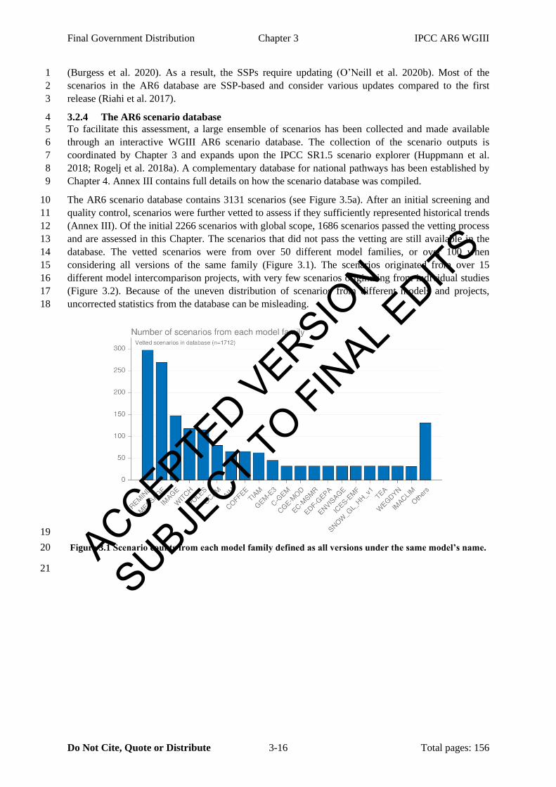
The AR6 scenario database contains 3131 scenarios (see Figure 3.5a). After an initial screening and 10
quality control, scenarios were further vetted to assess if they sufficiently represented historical trends 11
(Annex III). Of the initial 2266 scenarios with global scope, 1686 scenarios passed the vetting process 12
and are assessed in this Chapter. The scenarios that did not pass the vetting are still available in the 13
database. The vetted scenarios were from over 50 different model families, or over 100 when 14
considering all versions of the same family (Figure 3.1). The scenarios originated from over 15 15
different model intercomparison projects, with very few scenarios originating from individual studies 16
(Figure 3.2). Because of the uneven distribution of scenarios from different models and projects, 17
uncorrected statistics from the database can be misleading. 18
19
Figure 3.1 Scenario counts from each model family defined as all versions under the same model’s name. 20
21 ACCEPTED VERSIO
N
SUBJECT TO FIN
AL EDITS

Final Government Distribution Chapter 3 IPCC AR6 WGIII
Do Not Cite, Quote or Distribute 3-17 Total pages: 156
1
Figure 3.2 Scenario counts from each named project. 2
3
Each scenario with sufficient data is given a temperature classification using climate model emulators. 4
Three emulators were used in the assessment: FAIR (Smith et al. 2018), CICERO-SCM (Skeie et al. 5
2021), MAGICC (Meinshausen et al. 2020). Only the results of MAGICC are shown in this chapter as 6
it adequately covers the range of outcomes. The emulators are calibrated against the behaviour of 7
complex climate models and observation data, consistent with the outcomes of AR6 WGI AR6 (WGI 8
cross-chapter Box 7.1). The climate assessment is a three-step process of harmonization, infilling and 9
a probabilistic climate model emulator run (Annex III.2.5.1). Warming projections until the year 2100 10
were derived for 1574 scenarios, of which 1202 passed vetting, with the remaining scenarios having 11
insufficient information (Table 3.1 and Figure 3.3). For scenarios that limit warming to 2°C or below, 12
the SR15 classification was adopted in AR6, with more disaggregation provided for higher warming 13
levels (Table 3.1). These choices can be compared with the selection of common global warming 14
levels (GWL) of 1.5°C, 2°C, 3°C and 4°C to classify climate change impacts in the WGII assessment. 15
16
Table 3.1 Classification of emissions scenarios into warming levels using MAGICC 17
Description Subset WGI SSP
WGIII
IP
Scenarios
C1: Below 1.5°C with no or
limited overshoot <1.5°C peak warming with ≥33% chance and < 1.5°C
end of century warming with >50% chance SSP1-1.9
-, SP, LD,
Ren 97
C2: Below 1.5°C with high
overshoot <1.5°C peak warming with <33% chance and < 1.5°C
end of century warming with >50% chance 133
C3: Likely below 2°C <2°C peak warming with >67% chance SSP2-2.6
GS, Neg 311
C4: Below 2oC <2°C peak warming with >50% chance 159
C5: Below 2.5°C <2.5°C peak warming with >50% chance 212
ACCEPTED VERSION
SUBJECT TO FIN
AL EDITS

Final Government Distribution Chapter 3 IPCC AR6 WGIII
Do Not Cite, Quote or Distribute 3-18 Total pages: 156
C6: Below 3°C <3°C peak warming with >50% chance SSP2-4.5
Mod-Act 97
C7: Below 4°C <4°C peak warming with >50% chance SSP3-7.0
Cur-Pol 164
C8: Above 4°C >4°C peak warming with ≥50% chance SSP5-8.5 29
1
2
Figure 3.3 Of the 1686 scenarios that passed vetting, 1202 had sufficient data available to be classified 3 according to temperature, with an uneven distribution across warming levels. 4
In addition to the temperature classification, each scenario is assigned to one of the following policy 5
categories: (P0) diagnostic scenarios – 100 of 1686 vetted scenarios; (P1) scenarios with no globally 6
coordinated policy and either (P1a) no climate mitigation efforts – 119, (P1b) current national 7
mitigation efforts – 59, (P1c) Nationally Determined Contributions (NDCs) – 110, or (P1d) other non-8
standard assumptions – 104; (P2) globally coordinated climate policies with immediate (i.e. before 9
2030) action – 73, (P2a) without any transfer of emission permits – 435, (P2b) with transfers – 70; or 10
(P2c) with additional policy assumptions – 55; (P3) globally coordinated climate policies with 11
delayed (i.e. from 2030 onwards or after 2030) action, preceded by (P3a) no mitigation commitment 12
or current national policies – 7, (P3b) NDCs – 376, (P3c) NDCs and additional policies – 18 and 13
(P3d) other non-standard regional assumptions – 0; (P4) Cost-Benefit Analysis (CBA) – 2. The policy 14
categories were identified using text pattern matching on the scenario metadata and calibrated on the 15
best-known scenarios from model intercomparisons, with further validation against the related 16
literature, reported emission and carbon price trajectories, and exchanges with modellers. If the 17
information available is enough to qualify a policy category number but not sufficient for a 18
subcategory, then only the number is retained (e.g., P2 instead of P2a/b/c). A suffix added after P0 19
further qualifies a diagnostic scenario as one of the other policy categories.To demonstrate the 20
diversity of the scenarios, the vetted scenarios were classified into different categories along the 21
dimensions of population, GDP, energy, and cumulative emissions (Figure 3.4). The number of 22
scenarios in each category provides some insight into the current literature, but this does not indicate a 23
higher probability of that category occurring in reality. For population, the majority of scenarios are 24
consistent with the SSP2 ‘middle of the road’ category, with very few scenarios exploring the outer 25
ACCEPTED VERSION
SUBJECT TO FIN
AL EDITS
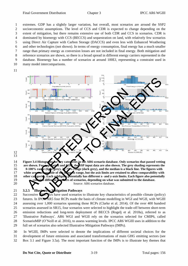
Final Government Distribution Chapter 3 IPCC AR6 WGIII
Do Not Cite, Quote or Distribute 3-19 Total pages: 156
extremes. GDP has a slightly larger variation, but overall, most scenarios are around the SSP2 1
socioeconomic assumptions. The level of CCS and CDR is expected to change depending on the 2
extent of mitigation, but there remains extensive use of both CDR and CCS in scenarios. CDR is 3
dominated by bioenergy with CCS (BECCS) and sequestration on land, with relatively few scenarios 4
using Direct Air Capture with Carbon Storage (DACCS) and even less with Enhanced Weathering 5
and other technologies (not shown). In terms of energy consumption, final energy has a much smaller 6
range than primary energy as conversion losses are not included in final energy. Both mitigation and 7
reference scenarios are shown, so there is a broad spread in different energy carriers represented in the 8
database. Bioenergy has a number of scenarios at around 100EJ, representing a constraint used in 9
many model intercomparisons. 10
11
12 13
Figure 3.4 Histograms for key categories in the AR6 scenario database. Only scenarios that passed vetting 14 are shown. For population and GDP, the SSP input data are also shown. The grey shading represents the 15
0-100% range (light grey), 25-75% range (dark grey), and the median is a black line. The figures with 16 white areas are outside of the scenario range, but the axis limits are retained to allow comparability with 17 other categories. Each subfigure potentially has different x- and y-axis limits. Each figure also potentially 18
contains different numbers of scenarios, depending on what was submitted to the database. 19 Source: AR6 scenarios database. 20
3.2.5 Illustrative Mitigation Pathways 21
Successive IPCC Ars have used scenarios to illustrate key characteristics of possible climate (policy) 22
futures. In IPCC AR5 four RCPs made the basis of climate modelling in WGI and WGII, with WGIII 23
assessing over 1,000 scenarios spanning those RCPs (Clarke et al. 2014). Of the over 400 hundred 24
scenarios assessed in SR15, four scenarios were selected to highlight the trade-off between short-term 25
emission reductions and long-term deployment of BECCS (Rogelj et al. 2018a), referred to as 26
‘Illustrative Pathways’. AR6 WGI and WGII rely on the scenarios selected for CMIP6, called 27
ScenarioMIP (O’Neill et al. 2016), to assess warming levels. IPCC AR6 WGIII uses in addition to the 28
full set of scenarios also selected Illustrative Mitigation Pathways (IMPs). 29
In WGIII, IMPs were selected to denote the implications of different societal choices for the 30
development of future emissions and associated transformations of main GHG emitting sectors (see 31
Box 3.1 and Figure 3.5a). The most important function of the IMPs is to illustrate key themes that 32
ACCEPTED VERSION
SUBJECT TO FIN
AL EDITS

Final Government Distribution Chapter 3 IPCC AR6 WGIII
Do Not Cite, Quote or Distribute 3-20 Total pages: 156
form a common thread in the report, both with a storyline and a quantitative illustration. The storyline 1
describes the key characteristics that define an IMP. The quantitative versions of the IMPs provide 2
numerical values that are internally consistent and comparable across chapters of the report. The 3
quantitative IMPs have been selected from the AR6 scenario database. No assessment of the 4
likelihood of each IMP has been made. 5
The selected scenarios (IPs) are divided into two sets (Figure 3.5 and Figure 3.6): two reference 6
pathways illustrative of high emissions and five Illustrative Mitigation Pathways (IMPs). The 7
narratives are explained in full in Annex III. The two reference pathways explore the consequences of 8
current policies and pledges: Current Policies (CurPol) and Moderate Action (ModAct). The CurPol 9
pathway explores the consequences of continuing along the path of implemented climate policies in 10
2020 and only a gradual strengthening after that. The scenario illustrates the outcomes of many 11
scenarios in the literature that project the outcomes of current policies. The ModAct pathway explores 12
the impact of implementing the Nationally Determined Contributions as formulated in 2020 and some 13
further strengthening after that. In line with current literature, these two reference pathways lead to an 14
increase in global mean temperature of more than 2°C (see Section 3.3). 15
The Illustrative Mitigation Pathways properly explore different pathways consistent with meeting the 16
long-term temperature goals of the Paris Agreement. They represent five different pathways that 17
emerge from the overall assessment. The IMPs consist of pathways with: gradual strengthening of 18
current policies (GS), extensive use of net negative emissions (Neg), renewables (Ren), low demand 19
(LD), and shifting pathways (SP). Each of these pathways can be implemented with different levels 20
of ambition. In the IMP framework, GS is consistent with staying likely below 2°C (C3), Neg shows a 21
strategy that also stays likely below 2°C level but returns to nearly 1.5°C by the end of the century 22
(hence indicated as C2*). The other variants that can limit warming to 1.5°C (C1) were selected. In 23
addition to these IMPs, sensitivity cases that explore alternative warming levels (C3) for Neg and Ren 24
are assessed (Neg-2.0 and Ren-2.0). 25
ACCEPTED VERSION
SUBJECT TO FIN
AL EDITS
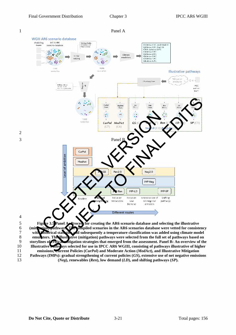
Final Government Distribution Chapter 3 IPCC AR6 WGIII
Do Not Cite, Quote or Distribute 3-21 Total pages: 156
Panel A 1
2
Panel B 3
4
Figure 3.5 Panel A: Process for creating the AR6 scenario database and selecting the illustrative 5 (mitigation) pathways. The compiled scenarios in the AR6 scenarios database were vetted for consistency 6
with historical statistics and subsequently a temperature classification was added using climate model 7 emulators. The illustrative (mitigation) pathways were selected from the full set of pathways based on 8
storylines of critical mitigation strategies that emerged from the assessment. Panel B: An overview of the 9 Illustrative Pathways selected for use in IPCC AR6 WGIII, consisting of pathways illustrative of higher 10
emissions, Current Policies (CurPol) and Moderate Action (ModAct), and Illustrative Mitigation 11 Pathways (IMPs): gradual strengthening of current policies (GS), extensive use of net negative emissions 12
(Neg), renewables (Ren), low demand (LD), and shifting pathways (SP). 13
ACCEPTED VERSION
SUBJECT TO FIN
AL EDITS
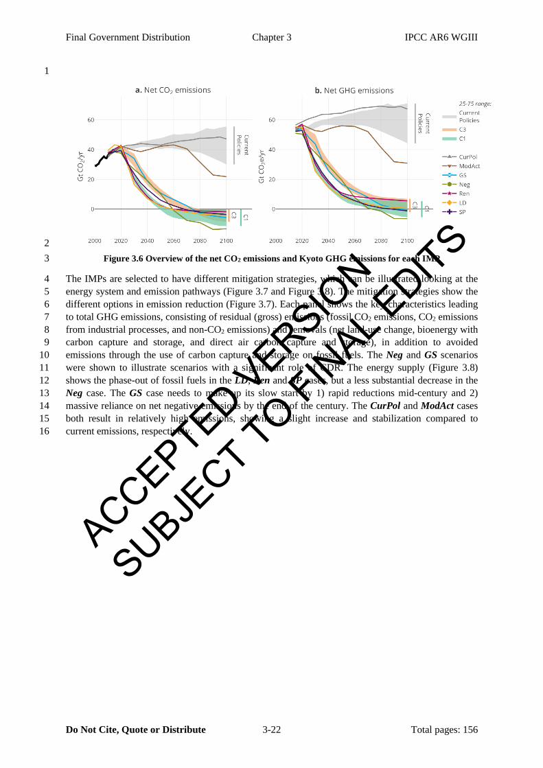
Final Government Distribution Chapter 3 IPCC AR6 WGIII
Do Not Cite, Quote or Distribute 3-22 Total pages: 156
1
2
Figure 3.6 Overview of the net CO2 emissions and Kyoto GHG emissions for each IMP 3
The IMPs are selected to have different mitigation strategies, which can be illustrated looking at the 4
energy system and emission pathways (Figure 3.7 and Figure 3.8). The mitigation strategies show the 5
different options in emission reduction (Figure 3.7). Each panel shows the key characteristics leading 6
to total GHG emissions, consisting of residual (gross) emissions (fossil CO2 emissions, CO2 emissions 7
from industrial processes, and non-CO2 emissions) and removals (net land-use change, bioenergy with 8
carbon capture and storage, and direct air carbon capture and storage), in addition to avoided 9
emissions through the use of carbon capture and storage on fossil fuels. The Neg and GS scenarios 10
were shown to illustrate scenarios with a significant role of CDR. The energy supply (Figure 3.8) 11
shows the phase-out of fossil fuels in the LD, Ren and SP cases, but a less substantial decrease in the 12
Neg case. The GS case needs to make up its slow start by 1) rapid reductions mid-century and 2) 13
massive reliance on net negative emissions by the end of the century. The CurPol and ModAct cases 14
both result in relatively high emissions, showing a slight increase and stabilization compared to 15
current emissions, respectively. 16
ACCEPTED VERSION
SUBJECT TO FIN
AL EDITS
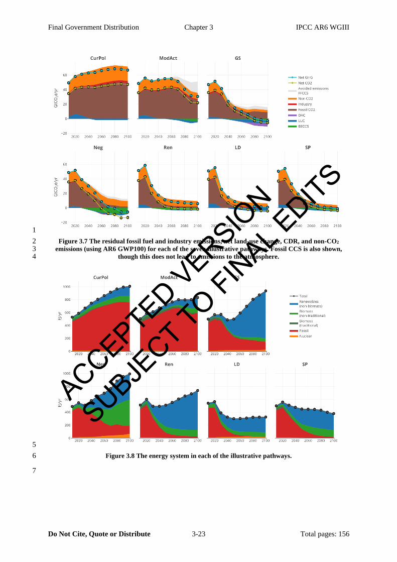
Final Government Distribution Chapter 3 IPCC AR6 WGIII
Do Not Cite, Quote or Distribute 3-23 Total pages: 156
1
Figure 3.7 The residual fossil fuel and industry emissions, net land-use change, CDR, and non-CO2 2 emissions (using AR6 GWP100) for each of the seven illustrative pathways. Fossil CCS is also shown, 3
though this does not lead to emissions to the atmosphere. 4
5
Figure 3.8 The energy system in each of the illustrative pathways. 6
7
ACCEPTED VERSION
SUBJECT TO FIN
AL EDITS

Final Government Distribution Chapter 3 IPCC AR6 WGIII
Do Not Cite, Quote or Distribute 3-24 Total pages: 156
3.3 Emission pathways, including socio-economic, carbon budget and 1
climate responses uncertainties 2
3.3.1 Socio-economic drivers of emissions scenarios 3
Greenhouse gas emissions mainly originate from the use and transformation of energy, agriculture, 4
land use (change) and industrial activities. The future development of these sources is influenced by 5
trends in socio-economic development, including population, economic activity, technology, politics, 6
lifestyles, and climate policy. Trends for these factors are not independent, and scenarios provide a 7
consistent outlook for these factors together (see Section 3.2). Marangoni et al. (2017) show that in 8
projections, assumptions influencing energy intensity (e.g., structural change, lifestyle and efficiency) 9
and economic growth are the most important determinants of future CO2 emissions from energy 10
combustion. Other critical factors include technology assumptions, preferences, resource assumptions 11
and policy (van Vuuren et al. 2008). As many of the factors are represented differently in specific 12
models, the model itself is also an important factor – providing a reason for the importance of model 13
diversity (Sognnaes et al. 2021). For land use, Stehfest et al. (2019) show that assumptions on 14
population growth are more dominant given that variations in per capita consumption of food are 15
smaller than for energy. Here, we only provide a brief overview of some key drivers. We focus first 16
on so-called reference scenarios (without stringent climate policy) and look at mitigation scenarios in 17
detail later. We use the SSPs to discuss trends in more detail. The SSPs were published in 2017, and 18
by now, some elements will have to be updated (O’Neill et al. 2020b). Still, the ranges represent the 19
full literature relatively well. 20
21
Historically, population and GDP have been growing over time. Scenario studies agree that further 22
global population growth is likely up to 2050, leading to a range of possible outcomes of around 8.5-23
11 billion people (see Figure 3.9). After 2050, projections show a much wider range. If fertility drops 24
below replacement levels, a decline in the global population is possible (as illustrated by SSP1 and 25
SSP5). This typically includes scenarios with rapid development and investment in education. 26
However, median projections mostly show a stabilisation of the world population (e.g., SSP2), while 27
high-end projections show a continued growth (e.g., SSP3). The UN Population Prospects include 28
considerably higher values for both the medium projection and the high end of the range than the SSP 29
scenarios (KC and Lutz 2017; UN 2019). The most recent median UN projection reaches almost 11 30
billion people in 2100. The key differences are in Africa and China: here, the population projections 31
are strongly influenced by the rate of fertility change (faster drop in SSPs). Underlying, the UN 32
approach is more based on current demographic trends while the SSPs assume a broader range of 33
factors (including education) driving future fertility. 34
35
Economic growth is even more uncertain than the population projections (Figure 3.9). The average 36
growth rate of GDP was about 2.8% per year (constant USD) in the 1990-2019 period (The World 37
Bank 2021). In 2020, the Covid-19 crisis resulted in a considerable drop in GDP (estimated around 4-38
5%) (IMF 2021). After a recovery period, most economic projections assume growth rates to 39
converge back to previous projections, although at a lower level (IMF 2021; OECD 2021) (see also 40
Box 3.2). In the long-term, assumptions on future growth relate to political stability, the role of the 41
progress of the technology frontier and the degree to which countries can catch up (Johansson et al. 42
2013). The SSP scenarios cover an extensive range, with low per capita growth in SSP3 and SSP4 43
(mostly in developing countries) and rapid growth in SSP1 and SSP5. At the same, however, also 44
scenarios outside the range have some plausibility – including the option of economic decline (Kallis 45
et al. 2012) or much faster economic development (Christensen et al. 2018). The OECD long-term 46
projection is at the global level reasonably consistent with SSP2. Equally important economic 47
parameters include income distribution (inequity) and the type of growth (structural change, i.e., 48
services vs manufacturing industries). Some projections (like SSP1) show a considerable convergence 49
of income levels within and across countries, while in other projections, this does not occur (e.g., 50
SSP3). Most scenarios reflect the suggested inverse relationship between the assumed growth rate for 51
income and population growth (Figure 3.9e). SSP1 and SSP5 represent examples of scenarios with 52
relatively low population increase and relatively high-income increase over the century. SSP3 53
ACCEPTED VERSION
SUBJECT TO FIN
AL EDITS

Final Government Distribution Chapter 3 IPCC AR6 WGIII
Do Not Cite, Quote or Distribute 3-25 Total pages: 156
represents an example of the opposite – while SSP2 and SSP4 are placed more in the middle. Nearly 1
all scenarios assessed here do not account for climate impacts on growth (mostly for methodological 2
reasons). As discussed in Section 3.5 these impacts can be considerable. An emerging area of 3
literature emphasises the possibility of stabilisation (or even decline) of income levels in developed 4
countries, arguing that such a trend would be preferred or even needed for environmental reasons 5
(Anderson and Larkin 2013; Kallis et al. 2020; Hickel and Kallis 2020; Keyßer and Lenzen 2021; 6
Hickel et al. 2021) (see also Chapter 5). Such scenarios are not common among IAM outcomes, that 7
are more commonly based on the idea that decarbonisation can be combined with economic growth 8
by a combination of technology, lifestyle and structural economic changes. Still, such scenarios could 9
result in a dramatic reduction of energy and resource consumption (see further). 10
11 Figure 3.9 Trends in key scenarios characteristics and driving forces as included in the SSP scenarios 12
(showing 5-95th percentiles of the reference scenarios as included in the database in grey shading). 13 Reference (dotted lines) refers to UN low, medium and high population scenario (UN 2019), OECD Long-14
term economic growth scenario (OECD 2021), the scenarios from IEA’s World Energy Outlook (IEA 15 2019), and the scenarios in the FAO assessment (FAO 2018) 16
Scenarios show a range of possible energy projections. In the absence of climate policy, most 17
scenarios project the final energy demand to continue to grow to around 650-800 EJ yr-1 in 2100 18
(based on the scenario database). Some projections show a very high energy demand up to 1000 EJ yr-19 1 (comparable to SSP5). The scenario of the IEA lies within the SSP range but near the SSP1 20
projection. However, it should be noted that the IEA scenario includes current policies (most 21
reference scenarios do not) and many scenarios published before 2021 did not account for the Covid-22
19 crisis. Several researchers discuss the possibility of decoupling material and energy demand from 23
ACCEPTED VERSION
SUBJECT TO FIN
AL EDITS
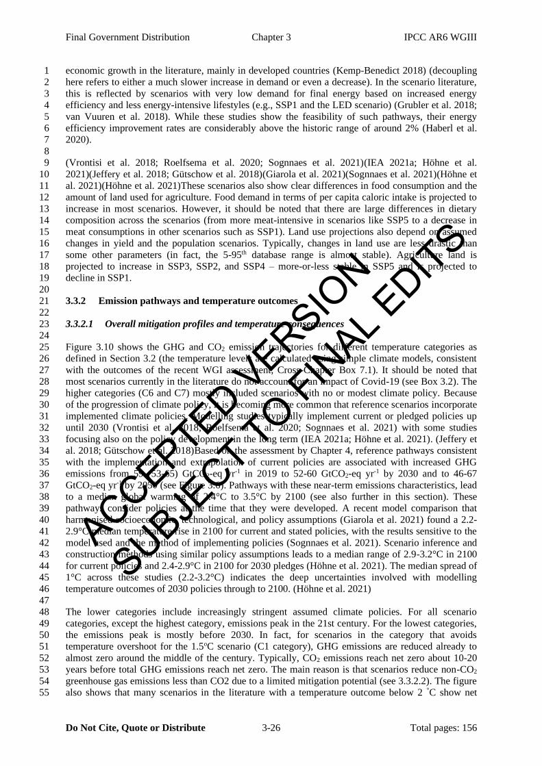
Final Government Distribution Chapter 3 IPCC AR6 WGIII
Do Not Cite, Quote or Distribute 3-26 Total pages: 156
economic growth in the literature, mainly in developed countries (Kemp-Benedict 2018) (decoupling 1
here refers to either a much slower increase in demand or even a decrease). In the scenario literature, 2
this is reflected by scenarios with very low demand for final energy based on increased energy 3
efficiency and less energy-intensive lifestyles (e.g., SSP1 and the LED scenario) (Grubler et al. 2018; 4
van Vuuren et al. 2018). While these studies show the feasibility of such pathways, their energy 5
efficiency improvement rates are considerably above the historic range of around 2% (Haberl et al. 6
2020). 7
8
(Vrontisi et al. 2018; Roelfsema et al. 2020; Sognnaes et al. 2021)(IEA 2021a; Höhne et al. 9
2021)(Jeffery et al. 2018; Gütschow et al. 2018)(Giarola et al. 2021)(Sognnaes et al. 2021)(Höhne et 10
al. 2021)(Höhne et al. 2021)These scenarios also show clear differences in food consumption and the 11
amount of land used for agriculture. Food demand in terms of per capita caloric intake is projected to 12
increase in most scenarios. However, it should be noted that there are large differences in dietary 13
composition across the scenarios (from more meat-intensive in scenarios like SSP5 to a decrease in 14
meat consumptions in other scenarios such as SSP1). Land use projections also depend on assumed 15
changes in yield and the population scenarios. Typically, changes in land use are less drastic than 16
some other parameters (in fact, the 5-95th database range is almost stable). Agriculture land is 17
projected to increase in SSP3, SSP2, and SSP4 – more-or-less stable in SSP5 and is projected to 18
decline in SSP1. 19
20
3.3.2 Emission pathways and temperature outcomes 21
22
3.3.2.1 Overall mitigation profiles and temperature consequences 23
24
Figure 3.10 shows the GHG and CO2 emission trajectories for different temperature categories as 25
defined in Section 3.2 (the temperature levels are calculated using simple climate models, consistent 26
with the outcomes of the recent WGI assessment, Cross-Chapter Box 7.1). It should be noted that 27
most scenarios currently in the literature do not account for an impact of Covid-19 (see Box 3.2). The 28
higher categories (C6 and C7) mostly included scenarios with no or modest climate policy. Because 29
of the progression of climate policy, it is becoming more common that reference scenarios incorporate 30
implemented climate policies. Modelling studies typically implement current or pledged policies up 31
until 2030 (Vrontisi et al. 2018; Roelfsema et al. 2020; Sognnaes et al. 2021) with some studies 32
focusing also on the policy development in the long term (IEA 2021a; Höhne et al. 2021). (Jeffery et 33
al. 2018; Gütschow et al. 2018)Based on the assessment by Chapter 4, reference pathways consistent 34
with the implementation and extrapolation of current policies are associated with increased GHG 35
emissions from 59 (53-65) GtCO2-eq yr-1 in 2019 to 52-60 GtCO2-eq yr-1 by 2030 and to 46-67 36
GtCO2-eq yr-1 by 2050 (see Figure 3.6). Pathways with these near-term emissions characteristics, lead 37
to a median global warming of 2.4°C to 3.5°C by 2100 (see also further in this section). These 38
pathways consider policies at the time that they were developed. A recent model comparison that 39
harmonised socioeconomic, technological, and policy assumptions (Giarola et al. 2021) found a 2.2-40
2.9°C median temperature rise in 2100 for current and stated policies, with the results sensitive to the 41
model used and the method of implementing policies (Sognnaes et al. 2021). Scenario inference and 42
construction methods using similar policy assumptions leads to a median range of 2.9-3.2°C in 2100 43
for current policies and 2.4-2.9°C in 2100 for 2030 pledges (Höhne et al. 2021). The median spread of 44
1°C across these studies (2.2-3.2°C) indicates the deep uncertainties involved with modelling 45
temperature outcomes of 2030 policies through to 2100. (Höhne et al. 2021) 46
47
The lower categories include increasingly stringent assumed climate policies. For all scenario 48
categories, except the highest category, emissions peak in the 21st century. For the lowest categories, 49
the emissions peak is mostly before 2030. In fact, for scenarios in the category that avoids 50
temperature overshoot for the 1.5oC scenario (C1 category), GHG emissions are reduced already to 51
almost zero around the middle of the century. Typically, CO2 emissions reach net zero about 10-20 52
years before total GHG emissions reach net zero. The main reason is that scenarios reduce non-CO2 53
greenhouse gas emissions less than CO2 due to a limited mitigation potential (see 3.3.2.2). The figure 54
also shows that many scenarios in the literature with a temperature outcome below 2 °C show net 55
ACCEPTED VERSION
SUBJECT TO FIN
AL EDITS

Final Government Distribution Chapter 3 IPCC AR6 WGIII
Do Not Cite, Quote or Distribute 3-27 Total pages: 156
negative emissions. There are, however, also exceptions in which more immediate emission 1
reductions limits the need for CDR. The IMPs illustrate alternative pathways to reach the C1-C3 2
temperature levels. 3
4
START BOX HERE 5
6
Box 3.2 Impact of Covid-19 on long-term emissions 7
8
The reduction in CO2 emissions of the Covid-19 pandemic in 2020 was estimated to be about 6% (see 9
section 4.2.2.4 and Table S4.2) lower than 2019 levels (BP 2021, Crippa et al. 2021, IEA 2021, Le 10
Quéré et al. 2021; Friedlingstein et al. 2020; Forster et al. 2020; Liu et al. 2020c). Near-real-time 11
monitoring estimates show a rebound in emissions levels, meaning 2021 emissions levels are 12
expected to be higher than 2020 (Le Quéré et al. 2021). The longer-term effects are uncertain but so 13
far do not indicate a clear structural change for climate policy related to the pandemic. The increase in 14
renewable shares in 2020 could stimulate a further transition, but slow economic growth can also slow 15
down (renewable) energy investments. Also, lifestyle changes during the crisis can still develop in 16
different directions (working from home, but maybe also living further away from work). Without a 17
major intervention, most long-term scenarios project that emission will start to follow a similar 18
pathway as earlier projections (although at a reduced level) (IEA 2020b; Kikstra et al. 2021a; 19
Rochedo et al. 2021). If emissions reductions are limited to only a short time, the adjustment of 20
pathways will lead to negligible outcomes in the order of 0.01K (Forster et al. 2020; Jones et al. 21
2021). At the same time, however, the large amount of investments pledged in the recovery packages 22
could provide a unique opportunity to determine the long-term development of infrastructure, energy 23
systems and land use (Hepburn et al. 2020; Pianta et al. 2021; Andrijevic et al. 2020b). Near-term 24
alternative recovery pathways have been shown to have the potential to influence carbon price 25
pathways, and energy investments and electrification requirements under stringent mitigation targets 26
(Kikstra et al. 2021a; Rochedo et al. 2021; Bertram et al. 2021; Pollitt et al. 2021; Shan et al. 2021). 27
Most studies suggest a noticeable reduction in 2030 emissions. However, much further reductions 28
would be needed to reach the emission levels consistent with mitigation scenarios that would likely 29
stay below 2oC or lower (see Chapter 4). At the moment, the share of investments in greenhouse gas 30
reduction is relatively small in most recovery packages, and no structural shifts for climate policies 31
are observed linked to the pandemic. Finally, most of the scenarios analysed in this Chapter do not 32
include the 2020 emissions reduction related to the Covid-19 pandemic. The effect of the pandemic 33
on the pathways will likely be very small. The assessment of climate mitigation pathways in this 34
chapter should be interpreted as being almost exclusively based on the assumption of a fast recovery 35
with limited persistent effects on emissions or structural changes. 36
37
END BOX HERE 38
39
ACCEPTED VERSION
SUBJECT TO FIN
AL EDITS

Final Government Distribution Chapter 3 IPCC AR6 WGIII
Do Not Cite, Quote or Distribute 3-28 Total pages: 156
1
Figure 3.10 Total emission profiles in the scenarios based on climate category for GHGs (AR6 GWP-100) 2 and CO2. The IMPs are also indicated 3
4
START BOX HERE 5
6
Box 3.3 The likelihood of high-end emission scenarios 7
8
At the time the Representative Concentration Pathways (RCPs) were published, they included 3 9
scenarios that could represent emission developments in the absence of climate policy: RCP4.5, RCP6 10
and RCP8.5, described as, respectively, low, medium and high-end scenarios in the absence of strong 11
climate policy (van Vuuren et al. 2011). RCP8.5 was described as representative of the top 5% 12
scenarios in the literature. The SSPs-based set of scenarios covered the RCP forcing levels adding a 13
new low scenario (at 1.9 W/m2). Hausfather and Peters (2020) pointed out that since 2011, the rapid 14
development of renewable energy technologies and emerging climate policy have made it 15
considerably less likely that emissions could end up as high as RCP8.5. Still, emission trends in 16
developing countries track RCP8.5 Pedersen et al. (2020), and high land-use emissions could imply 17
that emissions would continue to do so in the future, even at the global scale (Schwalm et al. 2020). 18
Other factors resulting in high emissions include higher population or economic growth as included in 19
the SSPs (see subsection 3.3.1) or rapid development of new energy services. Climate projections of 20
RCP8.5 can also result from strong feedbacks of climate change on (natural) emission sources and 21
high climate sensitivity (see WGI Chapter 7), and therefore their median climate impacts might also 22
materialise while following a lower emission path (e.g., Hausfather and Betts (2020)). The discussion 23
also relates to a more fundamental discussion on assigning likelihoods to scenarios, which is 24
extremely difficult given the deep uncertainty and direct relationship with human choice. However, it 25
would help to appreciate certain projections (e.g., Ho et al. (2019)). All-in-all, this means that high-26
end scenarios have become considerably less likely since AR5 but cannot be ruled out. It is important 27
to realize that RCP8.5 and SSP5-8.5 do not represent a typical ‘business-as-usual projection but are 28
only useful as high-end, high-risk scenarios. Reference emission scenarios (without additional climate 29
policy) typically end up in C5-C7 categories included in this assessment. 30
31
ACCEPTED VERSION
SUBJECT TO FIN
AL EDITS
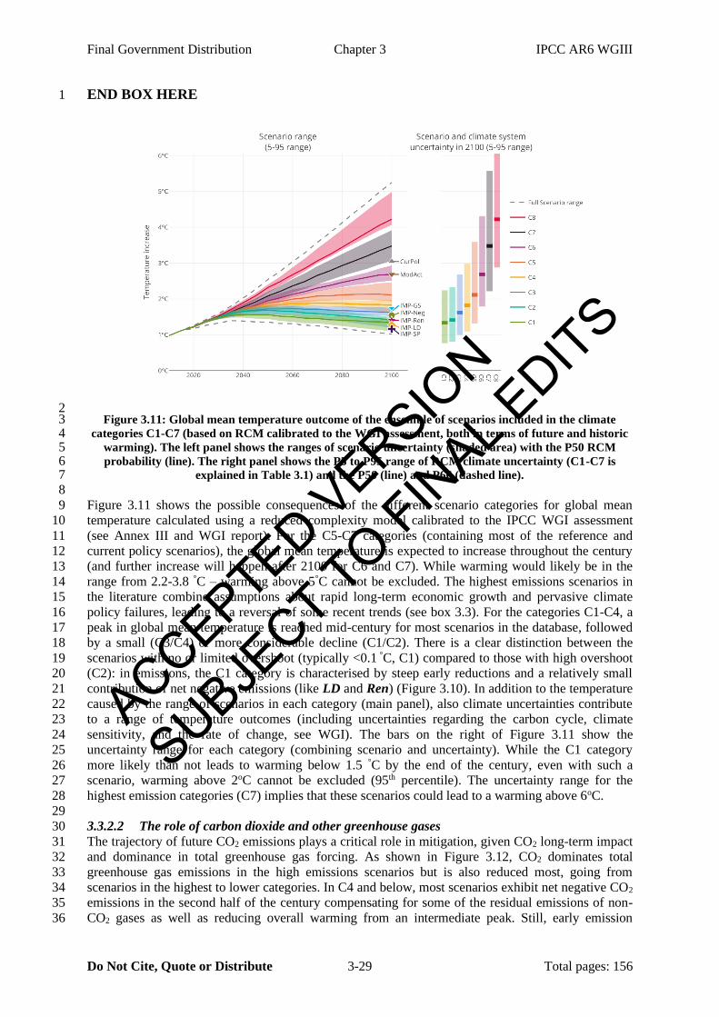
Final Government Distribution Chapter 3 IPCC AR6 WGIII
Do Not Cite, Quote or Distribute 3-29 Total pages: 156
END BOX HERE 1
2 Figure 3.11: Global mean temperature outcome of the ensemble of scenarios included in the climate 3
categories C1-C7 (based on RCM calibrated to the WGI assessment, both in terms of future and historic 4 warming). The left panel shows the ranges of scenario uncertainty (shaded area) with the P50 RCM 5 probability (line). The right panel shows the P5 to P95 range of RCM climate uncertainty (C1-C7 is 6
explained in Table 3.1) and the P50 (line) and P66 (dashed line). 7 8
Figure 3.11 shows the possible consequences of the different scenario categories for global mean 9
temperature calculated using a reduced complexity model calibrated to the IPCC WGI assessment 10
(see Annex III and WGI report). For the C5-C7 categories (containing most of the reference and 11
current policy scenarios), the global mean temperature is expected to increase throughout the century 12
(and further increase will happen after 2100 for C6 and C7). While warming would likely be in the 13
range from 2.2-3.8 °C – warming above 5°C cannot be excluded. The highest emissions scenarios in 14
the literature combine assumptions about rapid long-term economic growth and pervasive climate 15
policy failures, leading to a reversal of some recent trends (see box 3.3). For the categories C1-C4, a 16
peak in global mean temperature is reached mid-century for most scenarios in the database, followed 17
by a small (C3/C4) or more considerable decline (C1/C2). There is a clear distinction between the 18
scenarios with no or limited overshoot (typically <0.1 °C, C1) compared to those with high overshoot 19
(C2): in emissions, the C1 category is characterised by steep early reductions and a relatively small 20
contribution of net negative emissions (like LD and Ren) (Figure 3.10). In addition to the temperature 21
caused by the range of scenarios in each category (main panel), also climate uncertainties contribute 22
to a range of temperature outcomes (including uncertainties regarding the carbon cycle, climate 23
sensitivity, and the rate of change, see WGI). The bars on the right of Figure 3.11 show the 24
uncertainty range for each category (combining scenario and uncertainty). While the C1 category 25
more likely than not leads to warming below 1.5 °C by the end of the century, even with such a 26
scenario, warming above 2oC cannot be excluded (95th percentile). The uncertainty range for the 27
highest emission categories (C7) implies that these scenarios could lead to a warming above 6oC. 28
29
3.3.2.2 The role of carbon dioxide and other greenhouse gases 30
The trajectory of future CO2 emissions plays a critical role in mitigation, given CO2 long-term impact 31
and dominance in total greenhouse gas forcing. As shown in Figure 3.12, CO2 dominates total 32
greenhouse gas emissions in the high emissions scenarios but is also reduced most, going from 33
scenarios in the highest to lower categories. In C4 and below, most scenarios exhibit net negative CO2 34
emissions in the second half of the century compensating for some of the residual emissions of non-35
CO2 gases as well as reducing overall warming from an intermediate peak. Still, early emission 36
ACCEPTED VERSION
SUBJECT TO FIN
AL EDITS

Final Government Distribution Chapter 3 IPCC AR6 WGIII
Do Not Cite, Quote or Distribute 3-30 Total pages: 156
reductions and further reductions in non-CO2 emissions can also lead to scenarios without net 1
negative emissions in 2100, even in C1 and C3 (shown for the 85-95th percentile). In C1, avoidance of 2
significant overshoot implies that immediate gross reductions are more relevant than long-term net 3
negative emissions (explaining the lower number than in C2) but carbon dioxide removal is still 4
playing a role in compensating for remaining positive emissions in hard-to-abate sectors. 5
6
Figure 3.12 Upper left: The role of CO2 and other greenhouse gases. Emission in CO2-eq in 2100 (using 7 AR6 GWP-100) (other = halogenated gases) and upper right: Cumulative CO2 emissions in the 2020-2100 8
period. The lower left and right panel show the development of CH4 and N2O emissions over time. 9 Energy emissions include the contribution of BECCS. For both energy and AFOLU sectors, the positive 10 and negative values represent the cumulated annual balances. In both panels, the three bars per scenario 11 category represent the lowest 5-15th percentile, the average value and the highest 5-15th percentile. These 12
illustrate the range of scenarios in each category. The definition of C1-C7 can be found in Table 3.1 13
CH4 and N2O emissions are also reduced from C7 to C1, but this mostly occurs between C7 and C5. 14
The main reason is the characteristics of abatement potential: technical measures can significantly 15
reduce CH4 and N2O emissions at relatively low costs to about 50% of the current levels (e.g., by 16
reducing CH4 leaks from fossil fuel production and transport, reducing landfill emissions gazing, land 17
management and introducing measure related to manure management, see also Chapter 7 and 11). 18
However, technical potential estimates becomes exhausted even if the stringency of mitigation is 19
increased (Harmsen et al. 2019a,b; Höglund-Isaksson et al. 2020). Therefore, further reduction may 20
come from changes in activity levels, such as switching to a less meat-intensive diet reducing 21
livestock (Stehfest et al. 2009; Willett et al. 2019; Ivanova et al. 2020) (see also Chapter 7). Other 22
non-CO2 GHG emissions (halogenated gases) are reduced to low levels for scenarios below 2.5oC. 23
24
ACCEPTED VERSION
SUBJECT TO FIN
AL EDITS
Final Government Distribution Chapter 3 IPCC AR6 WGIII
Do Not Cite, Quote or Distribute 3-31 Total pages: 156
Short-lived climate forcers (SLCFs) also play an important role in climate change, certainly for short-1
term changes (see Figure SPM.2, WGI) (Shindell et al. 2012). These forcers consist of 1) substances 2
contributing to warming, such as methane, black carbon and tropospheric ozone and 2) substances 3
contributing to cooling (other aerosols, such as related to sulphur emissions). Most SLCFs are also air 4
pollutants, and reducing their emissions provides additional co-benefits (Shindell et al. 2017a,b; 5
Hanaoka and Masui 2020). In the case of the first group, emission reduction thus leads to both air 6
pollution and climate benefits. For the second, group there is a possible trade-off (Shindell and Smith 7
2019; Lund et al. 2020). As aerosol emissions are mostly associated with fossil fuel combustion, the 8
benefits of reducing CO2 could, in the short term, be reduced as a result of lower aerosol cooling. 9
There has been an active discussion on the exact climate contribution of SLCF focused policies in the 10
literature. This discussion partly emerged from different assumptions on possible reductions in the 11
absence of ambitious climate policy and the uncertain global climate benefit from aerosol (black 12
carbon) (Rogelj et al. 2014). The latter is now assessed to be smaller than originally thought (Smith et 13
al. 2020b; Takemura and Suzuki 2019) (see also WGI Chapter 6, Section 6.4). Reducing SLCF 14
emissions is critical to meet long-term climate goals and might help reduce the rate of climate change 15
in the short term. Deep SLCF emission reductions also increase the remaining carbon budget for a 16
specific temperature goal (Rogelj et al. 2015a; Reisinger et al. 2021) (see Box 3.4). A more detailed 17
discussion can be found in WGI Chapter 5 and 6. 18
19
For accounting of emissions and the substitution of different gases as part of a mitigation strategy, 20
typically, emission metrics are used to compare the climate impact of different gases. Most policies 21
currently use Global Warming Potentials with a 100-year time horizon as this is also mandated for 22
emissions reporting in the Paris Rulebook (for a wider discussion of GHG metrics, see Box 2.2 in 23
Chapter 2 and WGI, Chapter 7, Section 7.6). Alternative metrics have also been proposed, such as 24
those using a shorter or longer time horizon or those that focus directly on the consequences of 25
reaching a certain temperature target (Global Temperature Change Potential, GTP), allowing a more 26
direct comparison with cumulative CO2 emissions (Allen et al. 2016; Lynch et al. 2020) or focusing 27
on damages (Global Damage Potential) (an overview is given in Chapter 2, and Cross-Chapter Box 28
3). Depending on the metric, the value attributed to reducing short-lived forcers like methane can be 29
lower in the near term (e.g., in the case of GTP) or higher (GWP with short reference period). For 30
most metrics, however, the impact on mitigation strategies is relatively small, among others, due to 31
the marginal abatement cost curve of methane (low costs for low to medium mitigation levels; 32
expensive for high levels). The timing of reductions across different gases impacts warming and the 33
co-benefits (Harmsen et al. 2016; Cain et al. 2019). Nearly all scenarios in the literature use GWP-100 34
in cost-optimisation, reflecting the existing policy approach; the use of GWP-100 deviates from cost-35
optimal mitigation pathways by at most a few percent for temperature goals of likely below 2°C and 36
lower (see Box 2.2 in Chapter 2). 37
38
Cumulative CO2 emissions and temperature goals 39
The dominating role of CO2 and its long lifetime in the atmosphere and some critical characteristics of 40
the earth system implies that there is a strong relationship between cumulative CO2 emissions and 41
temperature outcomes (MacDougall and Friedlingstein 2015; Meinshausen et al. 2009; Allen et al. 42
2009; Matthews et al. 2009). This is illustrated in Figure 3.13 that plots the cumulative CO2 emissions 43
against the projected outcome for global mean temperature, both until a temperature peak and full 44
century. The deviations from in linear relationship in Figure 3.13 are mostly caused by different non-45
CO2 emission and forcing levels (see also Rogelj et al. (2015b)). This means that reducing non-CO2 46
emissions can play an important role in limiting peak warming: the smaller the residual non-CO2 47
warming, the larger the carbon budget. This impact on carbon budgets can be substantial for stringent 48
warming limits. For 1.5°C pathways, variations in non-CO2 warming across different emission 49
scenarios have been found to vary the remaining carbon budget by approximately 220 GtCO2 (see 50
WGI Chapter 5, Subsection 5.5.2.2). In addition to reaching net zero CO2 emissions, a strong 51
reduction in methane emissions is the most critical component in non-CO2 mitigation to keep the Paris 52
climate goals in reach (van Vuuren et al. 2018; Collins et al. 2018) (see also WGI, Chapter 5, 6 and 53
7). It should be noted that the temperature categories (C1-C7) generally aligned with the horizontal 54
axis, except for the end-of-century values for C1 and C2 that coincide. 55
ACCEPTED VERSION
SUBJECT TO FIN
AL EDITS

Final Government Distribution Chapter 3 IPCC AR6 WGIII
Do Not Cite, Quote or Distribute 3-32 Total pages: 156
START BOX HERE 1 2
Box 3.4 Consistency of remaining carbon budgets in the WGI assessment and cumulative CO2 3
emissions in WGIII mitigation pathways 4
Introduction 5
The WGI assessment has shown that the increase in global mean temperature has a near-linear 6
relationship with cumulative CO2 emissions (Chapter 5, Section 5.5, Box 5.3). Consistently, WGI has 7
confirmed that net zero CO2 emissions are required to halt CO2-induced warming. This permits the 8
estimation of carbon budgets consistent with specific temperature goals. In Chapter 3, we present the 9
temperature outcomes and cumulative CO2 emissions associated with different warming levels for 10
around 1200 scenarios published in the literature and which were classified according to different 11
warming levels (see Section 3.2 and Annex III, Part II.2.5). In this box, we discuss the consistency of 12
the assessments presented here and in IPCC WGI. The box summarises how the remaining carbon 13
budgets assessed by WGI relate to the remaining cumulative CO2 emissions until the time of net zero 14
CO2 emissions in mitigation pathways (Table 3.2, Table SPM1) assessed by WGIII. 15
16
In its assessment, WGI uses a framework in which the various components of the remaining carbon 17
budget are informed by various lines of evidence and assessed climate system characteristics. WGIII, 18
instead, uses around 1200 emission scenarios with estimated warming levels that cover the scenario 19
range presented in WGI but also contain many more intermediate projections with varying emission 20
profiles and a combination of CO2 emissions and other greenhouse gases. In order to assess their 21
climate outcomes, climate model emulators are used. The emulators are reduced complexity climate 22
models that are provided by WGI, and which are calibrated to the WGI assessment of future warming 23
for various purposes (a detailed description of the use of climate model emulators in the WGI and 24
WGIII assessments can be found in Cross-chapter Box 7.1 in the WGI report, with the connection of 25
WGI and WGII discussed in Annex III.2.5.1). 26
27
Remaining carbon budgets estimated by WGI 28
WGI estimated the remaining carbon budgets from their assessment of (i) the transient climate 29
response to cumulative emissions of carbon dioxide (TCRE), and estimates of (ii) the historical 30
human-induced warming, (iii) the temperature change after reaching net zero CO2 emissions, (iv) the 31
contribution of future non-CO2 warming (derived from the emissions scenarios assessed in the Special 32
Report on 1.5°C Warming using WGI-calibrated emulators), and (v) the earth system feedbacks (WGI 33
Chapter 5.5, Box 5.2). For a given warming level, WGI assessed the remaining carbon budget from 34
the beginning of 2020 onwards. These are 650 / 500 / 400 GtCO2 for limiting warming to 1.5°C with 35
33% / 50% / 67% chance and 1350 / 1150 GtCO2 for limiting warming to 2°C with 50% / 67% 36
chance. The estimates are subject to considerable uncertainty related to historical warming, future 37
non-CO2 forcing, and poorly quantified climate feedbacks. For instance, variation in non-CO2 38
emissions across scenarios are estimated to either increase or decrease the remaining carbon budget 39
estimates by 220 GtCO2. The estimates of the remaining carbon budget assume that non-CO2 40
emissions are reduced consistently with the tight temperature targets for which the budgets are 41
estimated. 42
43
Cumulative CO2 emissions until net zero estimated by WGIII 44
WGIII provides estimates of cumulative net CO2 emissions (from 2020 inclusive) until the time of 45
reaching net zero CO2 emissions (henceforth called “peak cumulative CO2 emissions”) and until the 46
end of the century for eight temperature classes that span a range of warming levels. The numbers can 47
be found in Table 3.2 (330-710 GtCO2 for C1; 540-930 for C2 and 640-1160 for C3). 48
49
Comparing the WGI remaining carbon budgets and remaining cumulative CO2 emissions of the 50
WGIII scenarios 51
A comparison between WGI and WGIII findings requires recognising that, unlike in WGI, cumulative 52
emissions in WGIII are not provided for a specific peak warming threshold or level but are instead 53
provided for a set of scenarios in a category, representing a specific range of peak temperature 54
ACCEPTED VERSION
SUBJECT TO FIN
AL EDITS

Final Government Distribution Chapter 3 IPCC AR6 WGIII
Do Not Cite, Quote or Distribute 3-33 Total pages: 156
outcomes (for instance the C4 category contains scenarios with a median peak warming anywhere 1
between approximately 1.8°C and up to 2°C). When accounting for this difference, the WGI and 2
WGIII findings are very consistent for temperature levels below 2oC. Figure 1 compares the peak 3
temperatures and associated cumulative CO2 emissions (i.e., peak cumulative CO2 emissions) for the 4
WGIII scenarios to the remaining carbon budgets assessed by WGI. This shows only minor 5
differences between the WGI and WGIII approaches. 6
7
8 9 Box 3.4 Figure 1: Cumulative CO2 emissions from AR6 scenario categories (coloured dots), adjusted for 10
distinct 0.1°C warming levels (black bars) in comparison to the WGI remaining carbon budgets (grey 11 bars). The cumulative carbon emissions for the AR6 scenarios are shown for the median peak warming 12
(panel a), the 33rd-percentile peak warming (panel b) and the upper 67th-percentile peak warming (panel 13 c) calculated with the WGI-calibrated emulator MAGICC7 (IPCC AR6 WGI, Cross-Chapter Box 7.1). 14 The adjustment to the nearest 0.1°C intervals is made using WGI TCRE (at the relevant percentile, e.g., 15
the 67th-percentile TCRE is used to adjust the 67th-percentile peak warming), with the 5% to 95% range 16 of adjusted scenarios provided by the black bar. The WGI remaining carbon budget is shown, including 17
the WGI estimate of at least a ±220 GtCO2 uncertainty due to non-CO2 emissions variations across 18 scenarios (grey bars). For median peak warming (panel a) projections below 2°C relative to 1850-1900, 19 the WGIII assessment of cumulative carbon emissions tends to be slightly smaller than the remaining 20 carbon budgets provided by WGI but well within the uncertainties. Note that only a few scenarios in 21
WGIII limit warming to below 1.5°C with a 50% chance, thus statistics for that specific threshold have 22 low confidence. 23
24 After correcting for the categorisation, some (small) differences between the WGI and WGIII 25
numbers arise from remaining differences between the outcomes of the climate emulators and their 26
set-up (see Cross-Chapter Box 7.1 in IPCC WGI AR6) and the differences in the underlying 27
scenarios. Moreover, the WGI assessment estimated the non-CO2 warming at the time of net zero CO2 28
emissions based on a relationship derived from the SR1.5 scenario database with historical emission 29
estimates as in Meinshausen et al. (2020) (WGI chapter 5). The WGIII assessment uses the same 30
climate emulator with improved historical emissions estimates (Nicholls et al. 2021) (WGI Cross-31
Chapter Box 7.1). Annex III.2.5.1 further explores the effects of these factors on the relationship 32
between non-CO2 warming at peak cumulative CO2 and peak surface temperature. 33
34
Estimates of the remaining carbon budgets thus vary with the assumed level of non-CO2 emissions, 35
which are a function of policies and technology development. The linear relationship used in the WGI 36
assessment between peak temperature and the warming as a result of non-CO2 emissions (based on 37
the SR1.5 data) is shown in the right panel of Figure 2 (dashed line). In the WG3 approach, the non-38
CO2 warming for each single scenario is based on the individual scenario characteristics. This shown 39
ACCEPTED VERSION
SUBJECT TO FIN
AL EDITS

Final Government Distribution Chapter 3 IPCC AR6 WGIII
Do Not Cite, Quote or Distribute 3-34 Total pages: 156
in the same figure by plotting the outcomes of scenario outcomes of a range models (dots). The lines 1
show the fitted data for individual models, emphasizing the clear differences across models and the 2
relationship with peak warming (policy level). In some scenarios stringent non-CO2 emission 3
reductions provide an option to reach more stringent climate goals with the same carbon budget. This 4
is especially the case for scenarios with a very low non-CO2 warming, for instance as a result of 5
methane reductions through diet change. The left panel shows how these differences impact estimates 6
of the remaining carbon budget. While the WGIII AR6 scenario database includes a broad range of 7
non-CO2 emission projections the overall range is still very consistent with the WGI relationship and 8
the estimated uncertainty with a ±220 GtCO2 range (see also panel B of Figure II.2 in Annex III.2.5). 9
10
11 Box 3.4 Figure 2: Panel A) Differences in regressions of the relationship between peak surface 12
temperature and associated cumulative CO2 emissions from 2020 derived from scenarios of eight 13 integrated assessment model frameworks. The coloured lines show the regression at median for scenarios 14 of the 8 modelling frameworks, each with more than 20 scenarios in the database and a detailed land-use 15
representation. The red dotted lines indicate the non-CO2 uncertainty range of WGI Chapter 5 (± 220 16 GtCO2), here visualised around the median of the 8 model framework lines. Carbon budgets from 2020 17
until 1.5C (0.43K above 2010-2019 levels) and 2.0C (0.93K above 2010-2019 levels) are shown for 18 minimum and maximum model estimates at the median, rounded to the nearest 10GtCO2. Panel B) 19
Shows the relationship between the estimated non-CO2 warming in mitigation scenarios that reach net 20 zero and the associated peak surface temperature outcomes. The coloured lines show the regression at 21 median for scenarios of the 8 modelling frameworks with more than 20 scenarios in the database and a 22
detailed land-use representation. The black dashed line indicates the non-CO2 relationship based on the 23 scenarios and climate emulator setup as was assessed in WGI Chapter 5. 24
Overall, the slight differences between the cumulative emissions in WGIII and the carbon budget in 25
WGI are because the non-CO2 warming in the WGIII AR6 scenarios is slightly lower than in the 26
SR1.5 scenarios that are used for the budget estimates in WGI (Annex III.2.5.1). In addition, 27
improved consistency with Cross-Chapter Box 7.1 in WGI results in a non-CO2 induced temperature 28
difference of about ~0.05K between the assessments. Re-calculating the remaining carbon budget 29
using the WGI methodology combined with the full WGIII AR6 scenario database results in a 30
reduction of the estimated remaining 1.5C carbon budget by about 100 GtCO2 (-20%), and a reduction 31
of ~40 GtCO2 (-3%) for 2C. Accounting also for the categorisation effect, the difference between the 32
WGI and WGIII estimates is found to be small and well within the uncertainty range (Figure 1). This 33
means that the cumulative CO2 emissions presented in WGIII and the WGI carbon budgets are highly 34
consistent. 35
ACCEPTED VERSION
SUBJECT TO FIN
AL EDITS

Final Government Distribution Chapter 3 IPCC AR6 WGIII
Do Not Cite, Quote or Distribute 3-35 Total pages: 156
A detailed comparison of the impact of different assessment steps, i.e., the new emulators, scenarios, 1
and harmonisation methods, has been made and is presented in Annex III. 2
3
Policy implications 4
The concept of a finite carbon budget means that the world needs to get to net zero CO2, no matter 5
whether global warming is limited to 1.5°C or well below 2°C (or any other level). Moreover, 6
exceeding the remaining carbon budget will have consequences by overshooting temperature levels. 7
Still, the relationship between the timing of net zero and temperature targets is a flexible one, as 8
discussed further in Cross-Chapter Box 3. It should be noted that national level inventory as used by 9
UNFCCC for the land use, land-use change and forestry sector are different from the overall concept 10
of anthropogenic emissions employed by IPCC WG1. For emissions estimates based on these 11
inventories, the remaining carbon budgets must be correspondingly reduced by approximately 15%, 12
depending on the scenarios (Grassi et al., 2021) (see also Chapter 7). 13
14
One of the uncertainties of the remaining carbon budget is the level of non-CO2 emissions which is a 15
function of policies and technology development. This represents a point of leverage for policies 16
rather than an inherent geophysical uncertainty. Stringent non-CO2 emission reductions hence can 17
provide – to some degree – an option to reach more stringent climate goals with the same carbon 18
budget. 19
20
END BOX HERE 21
22 Figure 3.13: The near-linear relationship between cumulative CO2 emissions and temperature. The left 23 panel shows cumulative emissions until net zero emission is reached. The right panel shows cumulative 24
emissions until the end of the century, plotted against peak and end-of-century temperature, respectively. 25 Both are shown as a function of non-CO2 forcing and cumulative net negative CO2 emissions. Position 26 temperature categories (circles) and IPs are also indicated, including two 2oC sensitivity cases for Neg 27
(Neg-2.0) and Ren (Ren-2.0). 28
The near-linear relationship implies that cumulative CO2 emissions are critically important for climate 29
outcomes (Collins et al. 2013). The maximum temperature increase is a direct function of the 30
cumulative emissions until net zero CO2 emissions is reached (the emission budget) (Figure 3.13, left 31
side). The end-of-century temperature correlates well with cumulative emissions across the century 32
ACCEPTED VERSION
SUBJECT TO FIN
AL EDITS
Final Government Distribution Chapter 3 IPCC AR6 WGIII
Do Not Cite, Quote or Distribute 3-36 Total pages: 156
(right panel). For long-term climate goals, positive emissions in the first half of the century can be 1
offset by net removal of CO2 from the atmosphere (net negative emissions) at the cost of a temporary 2
overshoot of the target (Tokarska et al. 2019). The bottom panels of Figure 3.13 show the contribution 3
of net negative CO2 emissions. 4
5
Focusing on cumulative emissions, the right-hand panel of Figure 3.12 shows that for high-end 6
scenarios (C6-C7), most emissions originate from fossil fuels, with a smaller contribution from net 7
deforestation. For C5 and lower, there is also a negative contribution to emissions from both AFOLU 8
emissions and energy systems. For the energy systems, these negative emissions originate from bio-9
energy-and-carbon-capture-and-storage (BECCS), while for AFOLU, they originate from re- and 10
afforestation. For C3-C5, reforestation has a larger CDR contribution than BECCS, mostly due to 11
considerably lower costs (Rochedo et al. 2018). For C1 and C2, the tight carbon budgets imply in 12
many scenarios more CDR use (Riahi et al. 2021). Please note that net negative emissions are not so 13
relevant for peak temperature targets, and thus the C1 category, but CDR can still be used to offset the 14
remaining positive emissions (Riahi et al. 2021). While positive CO2 emissions from fossil fuels are 15
significantly reduced, inertia and hard-to-abate sectors imply that in many C1-C3 scenarios, around 16
800-1000 GtCO2 of net positive cumulative CO2 emissions remain. This is consistent with literature 17
estimates that current infrastructure is associated with 650 GtCO2 (best estimate) if operated until the 18
end of its lifetime (Tong et al. 2019). These numbers are considerably above the estimated carbon 19
budgets for 1.5 °C estimated in WGI, hence explaining CDR reliance (either to offset emissions 20
immediately or later in time). 21
22
Creating net negative emissions can thus be an important part of a mitigation strategy to offset 23
remaining emissions or compensate for emissions earlier in time. As indicated above, there are 24
different ways to potentially achieve this, including re- and afforestation and BECCS (as often 25
covered in IAMs) but also soil carbon enhancement, direct air carbon capture and storage (DACCS) 26
and ocean alkalinization (see Chapter 12). Except for reforestation, these options have not been tested 27
at large scale and often require more R&D. Moreover, the reliance on CDR in scenarios has been 28
discussed given possible consequences of land use related to biodiversity loss and food security 29
(BECCS and afforestation), the reliance on uncertain storage potentials (BECCS and DACCS), water 30
use (BECCS), energy use (DACCS), the risks of possible temperature overshoot and the 31
consequences for meeting sustainable development goals (Venton 2016; Peters and Geden 2017; 32
Smith et al. 2016; van Vuuren et al. 2017; Anderson and Peters 2016; Honegger et al. 2021). In the 33
case of BECCS, it should be noted that bio-energy typically is associated with early-on positive CO2 34
emissions and net-negative effects are only achieved in time (carbon debt), and its potential is limited 35
(Cherubini et al. 2013; Hanssen et al. 2020) (most IAMs have only a very limited representation of 36
these time dynamics). Several scenarios have therefore explored how reliance on net negative CO2 37
emissions can be reduced or even avoided by alternative emission strategies (Grubler et al. 2018; van 38
Vuuren et al. 2018) or early reductions by more stringent emission reduction in the short-term (Rogelj 39
et al. 2019b; Riahi et al. 2021). A more in-depth discussion of land-based mitigation options can be 40
found in Chapter 7. It needs to be emphasized that even in strategies with net negative CO2 emissions, 41
the emission reduction via more conventional mitigation measures (efficiency improvement, 42
decarbonisation of energy supply) is much larger than the CDR contribution (Tsutsui et al. 2020). 43
44
3.3.2.3 The timing of net zero emissions 45
46
In addition to the constraints on change in global mean temperature, the Paris Agreement also calls for 47
reaching a balance of sources and sinks of GHG emissions (Art. 4). Different interpretations of the 48
concept related to balance have been published (Rogelj et al. 2015c; Fuglestvedt et al. 2018). Key 49
concepts include that of net zero CO2 emissions (anthropogenic CO2 sources and sinks equal zero) 50
and net zero greenhouse gas emission (see also Annex I Glossary and Box 3.3). The same notion can 51
be used for all GHG emissions, but here ranges also depend on the use of equivalence metrics 52
(Chapter 2, Box 2.2). Moreover, it should be noted that while reaching net zero CO2 emissions 53
typically coincides with the peak in temperature increase; net zero GHG emissions (based on GWP-54
100) implies a decrease in global temperature (Riahi et al. 2021) and net zero GHG emission typically 55
ACCEPTED VERSION
SUBJECT TO FIN
AL EDITS
Final Government Distribution Chapter 3 IPCC AR6 WGIII
Do Not Cite, Quote or Distribute 3-37 Total pages: 156
requires negative CO2 emissions to compensate for the remaining emissions from other GHGs. Many 1
countries have started to formulate climate policy in the year that net zero emissions (either CO2 or all 2
greenhouse gases) are reached – although, at the moment, formulations are often still vague (Rogelj et 3
al. 2021). There has been increased attention on the timing of net zero emissions in the scientific 4
literature and ways to achieve it. 5
6
Figure 3.14 shows that there is a relationship between the temperature target, the cumulative CO2 7
emissions budget, and the net zero year for CO2 emissions (left) and the sum of greenhouse gases 8
(right) for the scenarios published in the literature. In other words, the temperature targets from the 9
Paris Agreement can, to some degree, be translated into a net zero emission year (Tanaka and O’Neill 10
2018). There is, however, a considerable spread. In addition to the factors influencing the emission 11
budget (see WGI and section 3.3.2.2), this is influenced by the emission trajectory until net zero is 12
reached, decisions related to temperature overshoot and non-CO2 emissions (especially for the 13
moment CO2 reaches net zero emissions). Scenarios with limited or no net negative emissions and 14
rapid near-term emission reductions can allow small positive emissions (e.g., in hard-to-abate-15
sectors). They may therefore have a later year that net zero CO2 emissions are achieved. High 16
emissions in the short-term, in contrast, require an early net zero year. 17
18
For the scenarios in the C1 category (warming below 1.5°C (50% probability) with limited 19
overshoot), the net zero year for CO2 emissions is typically around 2035-2070 For scenarios in C3 20
(likely limiting warming to below 2°C), CO2 emissions reach net zero around 2060-2100. Similarly, 21
also the years for net zero GHG emissions can be calculated (see right graph). The GHG net zero 22
emissions year is typically around 10-20 years later than the carbon neutrality. Residual non-CO2 23
emissions at the time of reaching net zero CO2 range between 4-11 GtCO2-eq in pathways that likely 24
limit warming to 2.0°C or below. In pathways likely limiting warming to 2°C, methane is reduced by 25
around 20% (1-46%) in 2030 and almost 50% (26-64%) in 2050, and in pathways limiting warming to 26
1.5°C with no or limited overshoot by around 33% (19-57) in 2030 and a similar 50% (33-69%) in 27
2050. Emissions reduction potentials assumed in the pathways become largely exhausted when 28
limiting warming to below 2°C. N2O emissions are reduced too, but similar to CH4, emission 29
reductions saturate for stringent climate goals. In the mitigation pathways, the emissions of cooling 30
aerosols are reduced due to reduced use of fossil fuels. The overall impact on non-CO2-related 31
warming combines these factors. 32
In cost-optimal scenarios, regions will mostly achieve net zero emissions as a function of options for 33
emission reduction, CDR, and expected baseline emission growth (van Soest et al. 2021b). This 34
typically implies relatively early net zero emission years in scenarios for the Latin America region and 35
relatively late net zero years for Asia and Africa (and average values for OECD countries). However, 36
an allocation based on equity principles (such as responsibility, capability and equality) might result 37
in different carbon neutrality years, based on the principles applied – with often earlier net zero years 38
for the OECD (Fyson et al. 2020; van Soest et al. 2021b). Therefore, the emission trajectory until net 39
zero emissions is a critical determinant of future warming (see Section 3.5). The more CO2 is emitted 40
until 2030, the less CO2 can be emitted after that to stay below a warming limit (Riahi et al. 2015). As 41
discussed before, also non-CO2 forcing plays a key role in the short term. 42
43
START CCB HERE 44
45
Cross-Chapter Box 3: Understanding net zero CO2 and net zero GHG emissions 46
Authors: Elmar Kriegler (Germany), Alaa Al Khourdajie (United Kingdom/Syria), Edward Byers 47
(Ireland/Austria), Katherine Calvin (the United States of America), Leon Clarke (the United States of 48
America), Annette Cowie (Australia), Navroz Dubash (India), Jae Edmonds (the United States of 49
America), Jan S. Fuglestvedt (Norway), Oliver Geden (Germany), Giacomo Grassi (Italy/European 50
Union), Anders Hammer Strømman (Norway), Frank Jotzo (Australia), Alexandre Köberle 51
(Brazil/United Kingdom), Frank Lecocq (France), Yun Seng Lim (Malaysia), Eric Masanet (the 52
United States of America), Toshihiko Masui (Japan), Catherine Mitchell (United Kingdom), Gert-Jan 53
Nabuurs (the Netherlands), Anthony Patt (the United States of America/Switzerland), Glen Peters 54
ACCEPTED VERSION
SUBJECT TO FIN
AL EDITS

Final Government Distribution Chapter 3 IPCC AR6 WGIII
Do Not Cite, Quote or Distribute 3-38 Total pages: 156
(Australia/Norway), Andy Reisinger (New Zealand), Keywan Riahi (Austria), Joeri Rogelj (United 1
Kingdom/Belgium), Yamina Saheb (France/ Algeria), Jim Skea (United Kingdom), Detlef van 2
Vuuren (the Netherlands), Harald Winkler (Republic of South Africa) 3
4
This cross-chapter box surveys scientific, technical and policy aspects of net zero carbon dioxide 5
(CO2) and net zero greenhouse gas (GHG) emissions, with a focus on timing, the relationship with 6
warming levels, and sectoral and regional characteristics of net zero emissions. Assessment of net 7
zero GHG emissions additionally requires consideration of non-CO2 gases and choice of GHG 8
emission metrics used to aggregate emissions and removals of different GHGs (Cross-Chapter Box 2 9
in Chapter 2; Cross-Chapter Box 7 in Chapter 10). The following considers net zero CO2 and GHG 10
emissions globally, followed by regional and sectoral dimensions. 11
12
Net zero CO2 13
Reaching net zero CO2 emissions globally is necessary for limiting global warming to any level. 14
At the point of net zero CO2, the amount of CO2 human activity is putting into the atmosphere equals 15
the amount of CO2 human activity is removing from the atmosphere (see Glossary). Reaching and 16
sustaining net zero CO2 emissions globally stabilizes CO2-induced warming. Reaching net zero CO2 17
emissions and then moving to net negative CO2 emissions globally leads to a peak and decline in 18
CO2-induced warming (WGI AR6 Chapter 5.5, 5.6). 19
Limiting warming to 1.5°C or likely to 2°C requires deep, rapid, and sustained reductions of 20
other greenhouse gases including methane alongside rapid reductions of CO2 emissions to net 21
zero. This ensures that the warming contributions from non-CO2 forcing agents as well as from CO2 22
emissions are both limited at low levels. WGI estimated remaining carbon budgets until the time of 23
reaching net zero CO2 emissions for a range of warming limits, taking into account historical CO2 24
emissions and projections of the warming from non-CO2 forcing agents (WGI AR6 Chapter 5.5, 25
Cross-chapter box 3). 26
The earlier global net zero CO2 emissions are reached, the lower the cumulative net amount of 27
CO2 emissions and human-induced global warming, all else being equal (Figure 1a in this Box). 28
For a given net zero date, a variation in the shape of the CO2 emissions profile can lead to a variation 29
in the cumulative net amount of CO2 emissions until the time of net zero CO2 and as a result to 30
different peak warming levels. For example, cumulative net CO2 emissions until the time of reaching 31
net zero CO2 will be smaller, and peak warming lower, if emissions are reduced steeply and then more 32
slowly compared to reducing emissions slowly and then more steeply (Figure 1b in this Box). 33
Net zero CO2 emissions are reached between 2050-2055 (2035-2070) in global emissions 34
pathways limiting warming to 1.5°C with no or limited overshoot, and between 2070-2075 35
(2060-…) in pathways likely limiting warming to 2°C as reported in the AR6 scenario database 36
(median five-year interval and 5th-95th percentile ranges)3. The variation of non-CO2 emissions in 1.5-37
2°C pathways varies the available remaining carbon budget which can move the time of reaching net 38
zero CO2 in these pathways forward or backward4. The shape of the CO2 emissions reduction profile 39
FOOTNOTE 3 A small fraction of pathways in the AR6 scenarios database that likely limit warming to 2°C
(9%) or are as likely as not to limit warming to 2°C (14%) do not reach net-zero CO2 emissions during the 21st
century. This is not inconsistent with the fundamental scientific requirement to reach net-zero CO2 emissions for
a stable climate, but reflects that in some pathways, concurrent reductions in non-CO2 emissions temporarily
compensate for on-going warming from CO2 emissions. These would have to reach net-zero CO2 emissions
eventually after 2100 to maintain these warming limits. For the two classes of pathways, the 95th percentile
cannot be deduced from the scenario database as more than 5% of them do not reach net zero CO2 by 2100.
FOOTNOTE 4 WGI Chapter 5.5 estimates a variation of the remaining carbon budget by ± 220 GtCO2 due to
variations of the non-CO2 warming contribution in 1.5-2°C pathways. This translates to a shift of the timing of
ACCEPTED VERSION
SUBJECT TO FIN
AL EDITS

Final Government Distribution Chapter 3 IPCC AR6 WGIII
Do Not Cite, Quote or Distribute 3-39 Total pages: 156
also affects the time of reaching net zero CO2 (Figure 1c in this Box). Global emission pathways that 1
more than halve CO2 emissions from 2020 to 2030 can follow this rapid reduction by a more gradual 2
decline towards net zero CO2 and still limit warming to 1.5°C with no or limited overshoot, reaching 3
the point of net zero after 2050. The literature since SR1.5 included a larger fraction of such pathways 4
than were available at the time of SR1.5. This is the primary reason for the small backward shift in the 5
median estimate of reaching global net zero CO2 emissions in 1.5°C pathways collected in the AR6 6
scenario database compared to SR1.5. This does not mean that the world is assessed to have more 7
time to rapidly reduce current emissions levels compared to SR1.5. The assessment of emissions 8
reductions by 2030 and 2040 in pathways limiting warming to 1.5°C with no or limited overshoot has 9
not changed substantially. It only means that the exact timing of reaching net zero CO2 after a steep 10
decline of CO2 emissions until 2030 and 2040 can show some variation, and the SR1.5 median value 11
of 2050 is still close to the middle of the current range (Figure 1c in this Box ). 12
13
Cross-Chapter Box 3 Figure 1: Selected global CO2 emissions trajectories with similar shape and 14 different net zero CO2 date (Panel a), different shape and similar net zero CO2 date (Panel b), and similar 15
peak warming, but varying shapes and net zero CO2 dates (Panel c). Funnels show pathways limiting 16 warming to 1.5°C with no or limited overshoot (light blue) and likely limiting warming to 2°C (beige). 17
Historic CO2 emissions from Chapter 2.2 (EDGAR v6). 18
Pathways coinciding with emissions levels projected from the implementation of current NDCs 19
would result in substantially (>0.1°C) exceeding 1.5°C. They would have to reach net zero CO2 20
net zero CO2 by about ±10 years, assuming global CO2 emissions decrease linearly from current levels of
around 40 GtCO2 to net zero.
ACCEPTED VERSION
SUBJECT TO FIN
AL EDITS
Final Government Distribution Chapter 3 IPCC AR6 WGIII
Do Not Cite, Quote or Distribute 3-40 Total pages: 156
around 5-10 years later5 than in pathways with no or limited overshoot in order to reach the net 1
negative emissions that would then be required to return warming to 1.5°C by 2100. Those high 2
overshoot pathways have higher transient warming and higher reliance on net-negative CO2 emissions 3
towards the end of the 21st century. As they need to reach net zero CO2 only a few years later, with 4
2030 CO2 emission levels being around twice as high, they imply post-2030 CO2 emissions reduction 5
rates that are almost double that of pathways limiting warming to 1.5°C with no or limited overshoot 6
(Section 3.5). 7
Pathways following emissions levels projected from the implementation of current NDCs until 8
2030 would have to reach net zero CO2 around 10 years earlier6 than cost-effective pathways to 9
likely limit warming to 2°C. While cost-effective pathways take around 50-55 years to reach net 10
zero CO2 emissions, those pathways would only have 35-40 years left for transitioning to net zero 11
CO2 from 2030 onwards, close to the transition times that 1.5°C pathways are faced with today. 12
Current CO2 emissions and 2030 emission levels projected under the current NDCs are in a similar 13
range. (3.5, 4.2) 14
Net zero GHG emissions 15
The amount of CO2-equivalent emissions and the point when net zero GHG emissions are 16
reached in multi-GHG emissions pathways depends on the choice of GHG emissions metric. 17
Various GHG emission metrics are available for this purpose7. GWP100 is the most commonly used 18
metric for reporting CO2-equivalent emissions and is required for emissions reporting under the 19
Rulebook of the Paris Agreement. (Cross-Chapter Box 2 in Chapter 2, Annex II section 9, Annex I) 20
For most choices of GHG emissions metric, reaching net zero GHG emissions requires net 21
negative CO2 emissions in order to balance residual CH4, N2O and F-gas emissions. Under 22
foreseen technology developments, some CH4, N2O and F-gas emissions from, e.g., agriculture and 23
industry will remain over the course of this century. Net negative CO2 emissions will therefore be 24
needed to balance these remaining non-CO2 GHG emissions to obtain net zero GHG emissions at a 25
point in time after net zero CO2 has been reached in emissions pathways. Both the amount of net 26
negative CO2 emissions and the time lag to reaching net zero GHG depend on the choice of GHG 27
emission metric. 28
Reaching net zero GHG emissions globally in terms of GWP100 leads to a reduction in global 29
warming from an earlier peak. This is due to net negative CO2 emissions balancing the GWP100-30
equivalent emissions of short lived GHG emissions, which by themselves do not contribute to further 31
warming if sufficiently declining (Fuglestvedt et al. 2018; Rogelj et al. 2021). Hence, 1.5-2°C 32
FOOTNOTE 5 Pathways following emissions levels of current NDCs to 2030 and then returning median
warming to below 1.5°C in 2100 reach net zero during 2055-2060 (2045-2070) (median five year interval and
5th-95th percentile range).
FOOTNOTE 6 Pathways that follow emission levels projected from the implementation of current NDCs until
2030 and that still likely limit warming to 2°C reach net zero CO2 emissions during 2065 - 2070 (2060 - ...)
compared with 2075 - 2080 (2060 - …) in cost-effective pathways acting immediately to likely limit warming to
2°C (median five year interval and 5th-95th percentile range). See Footnote 1 for the lack of 95th percentile.
(Chapter 3.3 Table 3.1.)
FOOTNOTE 7 Defining net zero GHG emissions for a basket of greenhouse gases (GHGs) relies on a metric to
convert GHG emissions including methane (CH4), nitrous oxide (N2O), fluorinated gases (F-gases), and
potentially other gases, to CO2-equivalent emissions. The choice of metric ranges from Global Warming
Potentials (GWPs) and Global Temperature change Potentials (GTP) to economically-oriented metrics. All
metrics have advantages and disadvantages depending on the context in which they are used (Cross-Chapter
Box 2 in Chapter 2).
ACCEPTED VERSION
SUBJECT TO FIN
AL EDITS

Final Government Distribution Chapter 3 IPCC AR6 WGIII
Do Not Cite, Quote or Distribute 3-41 Total pages: 156
emissions pathways in the AR6 scenario database that reach global net zero GHG emissions in the 1
second half of the century show warming being halted at some peak value followed by a gradual 2
decline towards the end of the century (WGI Chapter 1 Box 1.4). 3
Global net zero GHG emissions measured in terms of GWP100 are reached between 2095-2100 4
(2055 - ...)8 in emission pathways limiting warming to 1.5°C with no or limited overshoot 5
(median and 5th-95th percentile). Around 50% of pathways limiting warming to 1.5°C with no or 6
limited overshoot and 70% of pathways limiting likely warming to 2°C do not reach net zero GHG 7
emissions in terms of GWP100 before 2100. These pathways tend to show less reduction in warming 8
after the peak than pathways that reach net zero GHG emissions. For the subset of pathways that 9
reach net zero GHG emissions before 2100, including 90% of pathways that return warming to 1.5°C 10
by 2100 after a high (>0.1°C) overshoot, the time lag between reaching net zero CO2 and net zero 11
GHG is 11-14 (6-40) years and the amount of net negative CO2 emissions deployed to balance non-12
CO2 emissions at the time of net zero is -6 to -7 (-10 to -4) GtCO2 (range of medians and lowest 5th 13
to highest 95 percentile across the four scenario classes that limit median warming to 2°C or lower). 14
(section 3.3, Table 3.1) 15
Sectoral and regional aspects of net zero 16
The timing of net zero CO2 or GHG emissions may differ across regions and sectors. Achieving 17
net zero emissions globally implies that some sectors and regions must reach net zero CO2 or 18
GHG ahead of the time of global net zero CO2 or GHG if others reach it later. Similarly, some 19
sectors and regions would need to achieve net negative CO2 or GHG emissions to compensate for 20
continued emissions by other sectors and regions after the global net zero year. Differences in the 21
timing to reach net zero emissions between sectors and regions depend on multiple factors, including 22
the potential of countries and sectors to reduce GHG emissions and undertake carbon dioxide 23
removal, the associated costs, and the availability of policy mechanisms to balance emissions and 24
removals between sectors and countries (Fyson et al. 2020; Strefler et al. 2021a; van Soest et al. 25
2021b). A lack of such mechanisms could lead to higher global costs to reach net zero emissions 26
globally, but less interdependencies and institutional needs (Fajardy and Mac Dowell 2020). Sectors 27
will reach net zero CO2 and GHG emissions at different times if they are aiming for such targets with 28
sector-specific policies or as part of an economy-wide net zero emissions strategy integrating 29
emissions reductions and removals across sectors. In the latter case, sectors with large potential for 30
achieving net-negative emissions would go beyond net zero to balance residual emissions from 31
sectors with low potential which in turn would take more time compared to the case of sector-specific 32
action. Global pathways project global AFOLU emissions to reach global net zero CO2 the earliest, 33
around 2030-2035 in pathways likely to limit warming to 2°C and below, by rapid reduction of 34
deforestation and enhancing carbon sinks on land, although net zero GHG emissions from global 35
AFOLU are typically reached 30 years later, if at all. The ability of global AFOLU CO2 emissions to 36
reach net zero as early as in the 2030s in modelled pathways hinges on optimistic assumptions about 37
the ability to establish global cost-effective mechanisms to balance emissions reductions and removals 38
across regions and sectors. These assumptions have been challenged in the literature and the Special 39
Report on Climate Change and Land (IPCC SRCCL). 40
The adoption and implementation of net zero CO2 or GHG emission targets by countries and 41
regions also depends on equity and capacity criteria. The Paris Agreement recognizes that peaking 42
of emissions will occur later in developing countries (Article 4.1). Just transitions to net zero CO2 or 43
GHG could be expected to follow multiple pathways, in different contexts. Regions may decide about 44
net zero pathways based on their consideration of potential for rapid transition to low-carbon 45
development pathways, the capacity to design and implement those changes, and perceptions of 46
equity within and across countries. Cost-effective pathways from global models have been shown to 47
FOOTNOTE 8 The 95th percentile cannot be deduced from the scenario database as more than 5% of pathways
do not reach net zero GHG by 2100 (Chapter 3.3 Table 3.1.), hence denoted by -…
ACCEPTED VERSION
SUBJECT TO FIN
AL EDITS
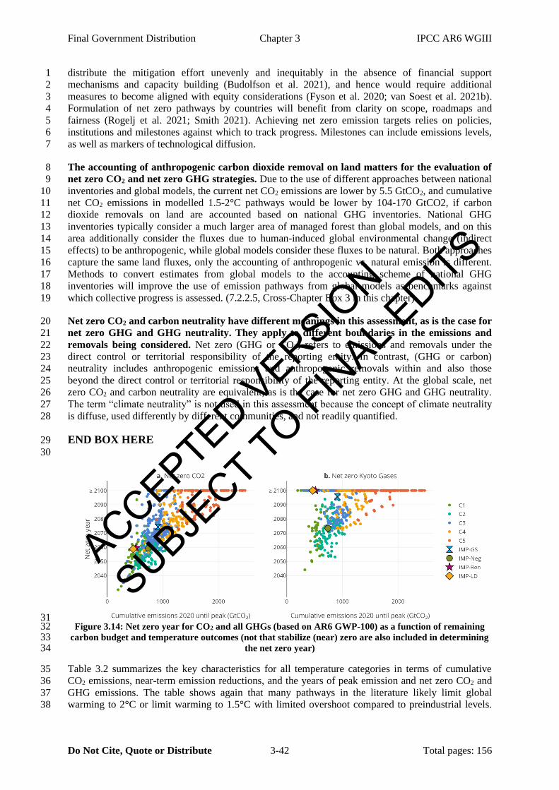
Final Government Distribution Chapter 3 IPCC AR6 WGIII
Do Not Cite, Quote or Distribute 3-42 Total pages: 156
distribute the mitigation effort unevenly and inequitably in the absence of financial support 1
mechanisms and capacity building (Budolfson et al. 2021), and hence would require additional 2
measures to become aligned with equity considerations (Fyson et al. 2020; van Soest et al. 2021b). 3
Formulation of net zero pathways by countries will benefit from clarity on scope, roadmaps and 4
fairness (Rogelj et al. 2021; Smith 2021). Achieving net zero emission targets relies on policies, 5
institutions and milestones against which to track progress. Milestones can include emissions levels, 6
as well as markers of technological diffusion. 7
The accounting of anthropogenic carbon dioxide removal on land matters for the evaluation of 8
net zero CO2 and net zero GHG strategies. Due to the use of different approaches between national 9
inventories and global models, the current net CO2 emissions are lower by 5.5 GtCO2, and cumulative 10
net CO2 emissions in modelled 1.5-2°C pathways would be lower by 104-170 GtCO2, if carbon 11
dioxide removals on land are accounted based on national GHG inventories. National GHG 12
inventories typically consider a much larger area of managed forest than global models, and on this 13
area additionally consider the fluxes due to human-induced global environmental change (indirect 14
effects) to be anthropogenic, while global models consider these fluxes to be natural. Both approaches 15
capture the same land fluxes, only the accounting of anthropogenic vs. natural emission is different. 16
Methods to convert estimates from global models to the accounting scheme of national GHG 17
inventories will improve the use of emission pathways from global models as benchmarks against 18
which collective progress is assessed. (7.2.2.5, Cross-Chapter Box 3 in this chapter) 19
Net zero CO2 and carbon neutrality have different meanings in this assessment, as is the case for 20
net zero GHG and GHG neutrality. They apply to different boundaries in the emissions and 21
removals being considered. Net zero (GHG or CO2) refers to emissions and removals under the 22
direct control or territorial responsibility of the reporting entity. In contrast, (GHG or carbon) 23
neutrality includes anthropogenic emissions and anthropogenic removals within and also those 24
beyond the direct control or territorial responsibility of the reporting entity. At the global scale, net 25
zero CO2 and carbon neutrality are equivalent, as is the case for net zero GHG and GHG neutrality. 26
The term “climate neutrality” is not used in this assessment because the concept of climate neutrality 27
is diffuse, used differently by different communities, and not readily quantified. 28
END BOX HERE 29
30
31 Figure 3.14: Net zero year for CO2 and all GHGs (based on AR6 GWP-100) as a function of remaining 32
carbon budget and temperature outcomes (not that stabilize (near) zero are also included in determining 33 the net zero year) 34
Table 3.2 summarizes the key characteristics for all temperature categories in terms of cumulative 35
CO2 emissions, near-term emission reductions, and the years of peak emission and net zero CO2 and 36
GHG emissions. The table shows again that many pathways in the literature likely limit global 37
warming to 2°C or limit warming to 1.5°C with limited overshoot compared to preindustrial levels. 38
ACCEPTED VERSION
SUBJECT TO FIN
AL EDITS
Final Government Distribution Chapter 3 IPCC AR6 WGIII
Do Not Cite, Quote or Distribute 3-43 Total pages: 156
Cumulative net CO2 emissions from the year 2020 until the time of net zero CO2 in pathways that 1
limit warming to 1.5°C with no or limited overshoot are 510 (330-710) GtCO2 and in pathways likely 2
to limit warming to below 2.0°C 890 (640-1160) GtCO2 (see also Cross-Chapter Box 3 in this 3
chapter). Mitigation pathways likely to limit global warming to 2°C compared to pre-industrial levels 4
are associated with net global GHG emissions of 40 (32–55) GtCO2-eq yr-1 by 2030 and 20 (13-26) 5
GtCO2-eq yr-1 in 2050. These correspond to GHG emissions reductions of 21 (1-42) % by 2030, and 6
64 (53-77) % by 2050 relative to 2019 emission levels. Pathways that limit global warming to below 7
1.5°C with no or limited overshoot require a further acceleration in the pace of the transformation, 8
with GHG emissions reductions of 43 (34–60) % by 2030 and 84 (74–98) % in 2050 relative to 9
modelled 2019 emission levels. The likelihood of limiting warming to below 1.5°C with no or limited 10
overshoot of the most stringent mitigation pathways in the literature (C1) has declined since SR1.5. 11
This is because emissions have risen since 2010 by about 9 GtCO2 yr-1, resulting in relatively higher 12
near-term emissions of the AR6 pathways by 2030 and slightly later dates for reaching net zero CO2 13
emissions compared to SR1.5 14
15
Given the larger contribution of scenarios in the literature that aim to reduce net-negative emissions, 16
emission reductions are somewhat larger in the short-term compared to similar categories in the IPCC 17
SR1.5. At the same time, the year of net zero emissions is somewhat later (but only if these rapid, 18
short-term emission reductions are achieved). The scenarios in the literature in C1-C3 show a peak in 19
global emissions before 2025. Not achieving this requires a more rapid reduction after 2025 to still 20
meet the Paris goals (see Section 3.5). 21
22
ACCEPTED VERSION
SUBJECT TO FIN
AL EDITS
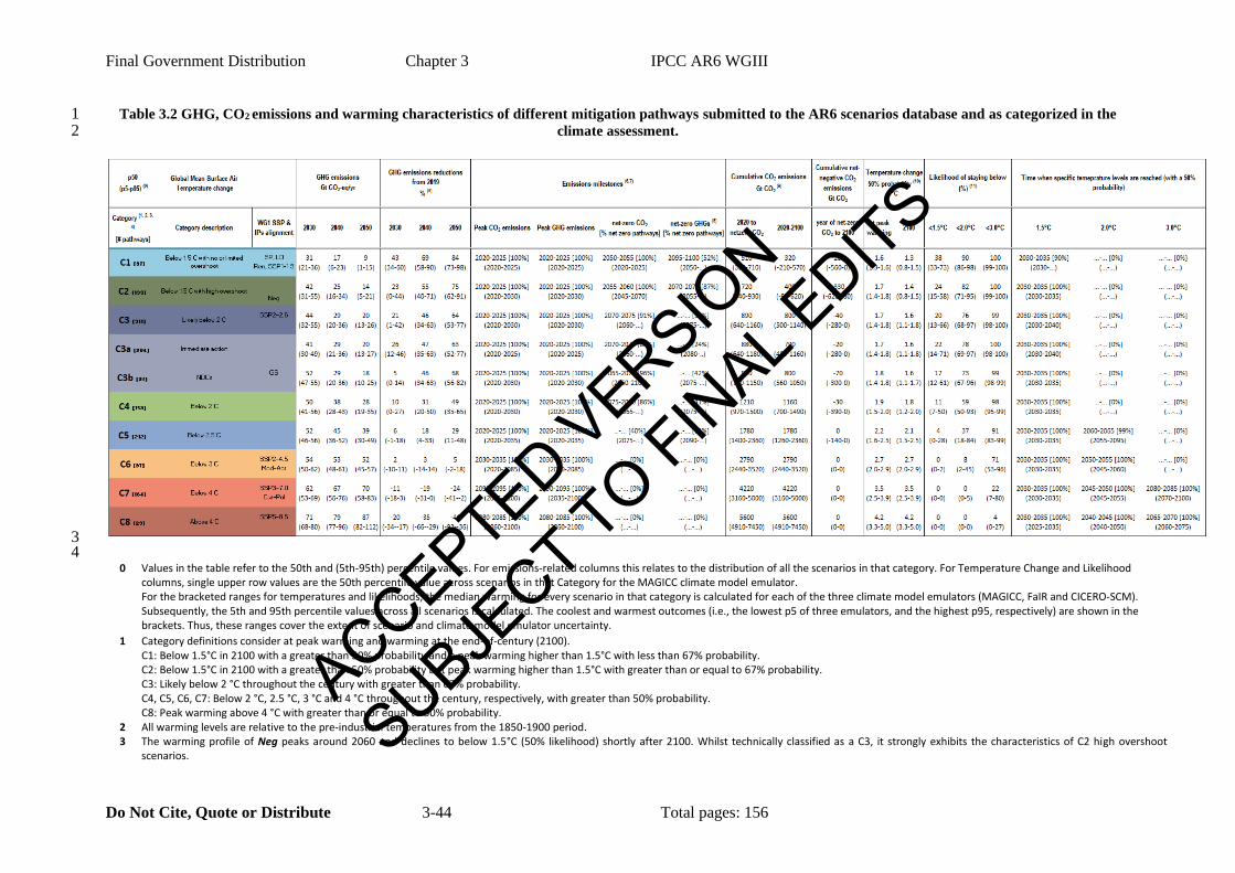
Final Government Distribution Chapter 3 IPCC AR6 WGIII
Do Not Cite, Quote or Distribute 3-44 Total pages: 156
Table 3.2 GHG, CO2 emissions and warming characteristics of different mitigation pathways submitted to the AR6 scenarios database and as categorized in the 1 climate assessment. 2
3 4
0 Values in the table refer to the 50th and (5th-95th) percentile values. For emissions-related columns this relates to the distribution of all the scenarios in that category. For Temperature Change and Likelihood columns, single upper row values are the 50th percentile value across scenarios in that Category for the MAGICC climate model emulator. For the bracketed ranges for temperatures and likelihoods, the median warming for every scenario in that category is calculated for each of the three climate model emulators (MAGICC, FaIR and CICERO-SCM). Subsequently, the 5th and 95th percentile values across all scenarios is calculated. The coolest and warmest outcomes (i.e., the lowest p5 of three emulators, and the highest p95, respectively) are shown in the brackets. Thus, these ranges cover the extent of scenario and climate model emulator uncertainty.
1 Category definitions consider at peak warming and warming at the end-of-century (2100). C1: Below 1.5°C in 2100 with a greater than 50% probability and a peak warming higher than 1.5°C with less than 67% probability. C2: Below 1.5°C in 2100 with a greater than 50% probability but peak warming higher than 1.5°C with greater than or equal to 67% probability. C3: Likely below 2 °C throughout the century with greater than 67% probability. C4, C5, C6, C7: Below 2 °C, 2.5 °C, 3 °C and 4 °C throughout the century, respectively, with greater than 50% probability. C8: Peak warming above 4 °C with greater than or equal to 50% probability.
2 All warming levels are relative to the pre-industrial temperatures from the 1850-1900 period. 3 The warming profile of Neg peaks around 2060 and declines to below 1.5°C (50% likelihood) shortly after 2100. Whilst technically classified as a C3, it strongly exhibits the characteristics of C2 high overshoot
scenarios.
ACCEPTED VERSION
SUBJECT TO FIN
AL EDITS
Final Government Distribution Chapter 3 IPCC AR6 WGIII
Do Not Cite, Quote or Distribute 3-45 Total pages: 156
4 C3 scenarios are sub-categorized according to policy ambition and consistent with Figure SPM 6. Hence the subtotals of C3a & C3b do not match the total of C3 scenarios, as there areC3 scenarios with policy categorizations not covered by C3a and C3b.
5 Percentage GHG reduction ranges shown here compare 2019 estimates from historical emissions assessed in Chapter 2 (58 Gt CO2) to the harmonized and infilled projections from the models. Negative values (e.g., in C7, C8) represent an increase in emissions.
6 Gross, % reductions and emissions milestones are based on model data for CO2 & GHG emissions, which has been harmonized to 2015 values. See also Footnote 6.
7 Percentiles reported across all pathways in that category including pathways that do not reach net zero before 2100 (fraction in square brackets). If the fraction of pathways that reach net zero before 2100 (one minus fraction in square brackets) is lower than the fraction of pathways covered by a percentile (e.g., 0.95 for the 95th percentile), the percentile is not defined and denoted with "…".
8 For cases where models do not report all GHGs, missing GHG species are infilled and calculated as Kyoto basket with AR6 GWP-100 CO2-equivalent factors. For each scenario, a minimum of native reporting of CO2, CH4, and N2O emissions to 2100 was required for the assessment of the climate response and assignment to a climate category. Emissions scenarios without climate assessment are not included in the ranges. See Annex III.
9 For better comparability with the WGI assessment of the remaining carbon budget, the cumulative CO2 emissions of the pathways are harmonized to the 2015 CO2 emissions levels used in the WGI assessment and are calculated for the future starting on 1 January 2020.
10 Temperature change (Global Surface Air Temperature - GSAT) for category (at peak and in 2100), based on the median warming for each scenario assessed using the probabilistic climate model emulators. 11 Probability of staying below the temperature thresholds for the scenarios in each category, taking into consideration the range of uncertainty from the climate model emulators consistent with the WGI AR6
assessment. The probabilities refer to the probability at peak temperature. Note that in the case of temperature overshoot (E.g., category C2 and some scenarios in C1), the probabilities at the end of the century are higher than the probability at peak temperature.
ACCEPTED VERSION
SUBJECT TO FIN
AL EDITS
Final Government Distribution Chapter 3 IPCC AR6 WGIII
Do Not Cite, Quote or Distribute 3-46 Total pages: 156
3.3.2.4 Mitigation strategies 1
Detailed sectoral implications are discussed in Section 3.4 and Chapters 5-11 (see also Table 3.3). The 2
stringency of climate policy has clear implications for mitigation action (Figure 3.15). There are a 3
number of important commonalities of pathways likely limiting warming to 2C and below: for 4
instance, they all rely on significant improvement of energy efficiency, rapid decarbonisation of 5
supply and, many of them, CDR (in energy supply or AFOLU), either in terms of net negative 6
emissions or to compensate residual emissions. Still, there are also important differences and the 7
(IMPs) show how different choices can steer the system into alternative directions with different 8
combinations of response options. For decarbonisation of energy supply many options exist, including 9
CCS, nuclear power, and renewables (see Chapter 6). In the majority of the scenarios reaching low 10
greenhouse targets, a considerable amount of CCS is applied (panel d). The share of renewables is 11
around 30-70% in the scenarios reaching a global average temperature change of likely below 2oC and 12
clearly above 40% for scenarios reaching 1.5oC (panel c). Scenarios have been published with 100% 13
renewable energy systems even at a global scale, partly reflecting the rapid progress made for these 14
technologies in the last decade (Breyer and Jefferson 2020; Creutzig et al. 2017; Jacobson et al. 2018). 15
These scenarios do not show in the graph due to a lack of information from non-energy sources. There 16
is a debate in the literature on whether it is possible to achieve a 100% renewable energy system by 17
2050 (Brook et al. 2018). This critically depends on assumptions made on future system integration, 18
system flexibility, storage options, consequences for material demand and the ability to supply high-19
temperature functions and specific mobility functions with renewable energy. The range of studies 20
published showing 100% renewable energy systems show that it is possible to design such systems in 21
the context of energy system models (Lehtveer and Hedenus 2015a,b; Hong et al. 2014a,b; Zappa et 22
al. 2019; Pfenninger and Keirstead 2015; Sepulveda et al. 2018; IEA 2021b) (see also Box 6.6 in 23
Chapter 6 on 100% renewables in net zero CO2 systems). Panel e and f, finally, show the contribution 24
of CDR – both in terms of net negative emissions and gross CDR. The contribution of total CDR 25
obviously exceeds the net negative emissions. It should be noted that while a majority of scenarios 26
relies on net negative emissions to reach stringent mitigation goals – this is not the case for all of 27
them. 28
ACCEPTED VERSION
SUBJECT TO FIN
AL EDITS
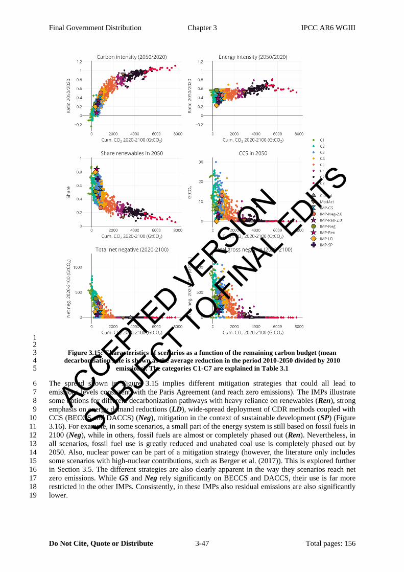
Final Government Distribution Chapter 3 IPCC AR6 WGIII
Do Not Cite, Quote or Distribute 3-47 Total pages: 156
1 2
Figure 3.15: Characteristics of scenarios as a function of the remaining carbon budget (mean 3 decarbonisation rate is shown as the average reduction in the period 2010-2050 divided by 2010 4
emissions). The categories C1-C7 are explained in Table 3.1 5
The spread shown in Figure 3.15 implies different mitigation strategies that could all lead to 6
emissions levels consistent with the Paris Agreement (and reach zero emissions). The IMPs illustrate 7
some options for different decarbonization pathways with heavy reliance on renewables (Ren), strong 8
emphasis on energy demand reductions (LD), wide-spread deployment of CDR methods coupled with 9
CCS (BECCS and DACCS) (Neg), mitigation in the context of sustainable development (SP) (Figure 10
3.16). For example, in some scenarios, a small part of the energy system is still based on fossil fuels in 11
2100 (Neg), while in others, fossil fuels are almost or completely phased out (Ren). Nevertheless, in 12
all scenarios, fossil fuel use is greatly reduced and unabated coal use is completely phased out by 13
2050. Also, nuclear power can be part of a mitigation strategy (however, the literature only includes 14
some scenarios with high-nuclear contributions, such as Berger et al. (2017)). This is explored further 15
in Section 3.5. The different strategies are also clearly apparent in the way they scenarios reach net 16
zero emissions. While GS and Neg rely significantly on BECCS and DACCS, their use is far more 17
restricted in the other IMPs. Consistently, in these IMPs also residual emissions are also significantly 18
lower. 19
ACCEPTED VERSION
SUBJECT TO FIN
AL EDITS

Final Government Distribution Chapter 3 IPCC AR6 WGIII
Do Not Cite, Quote or Distribute 3-48 Total pages: 156
1
Figure 3.16: Primary energy use and net emissions at net zero year for the different IMPS 2
Mitigation pathways also have a regional dimension. In 2010, about 40% of emissions originated 3
from the Developed Countries and Eastern Europe and west-central Asia regions. According to the 4
projections shown in 5
6 Figure 3.17, the share of the latter regions will further increase to about 70% by 2050. In the scenarios 7
in the literature, emissions are typically almost equally reduced across the regions. 8
9
ACCEPTED VERSION
SUBJECT TO FIN
AL EDITS
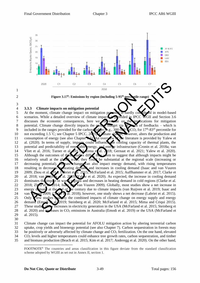
Final Government Distribution Chapter 3 IPCC AR6 WGIII
Do Not Cite, Quote or Distribute 3-49 Total pages: 156
1
Figure 3.179: Emissions by region (including 5-95th percentile range) 2
3
3.3.3 Climate impacts on mitigation potential 4
At the moment, climate change impact on mitigation potential is hardly considered in model-based 5
scenarios. While a detailed overview of climate impacts is provided in IPCC WGII and Section 3.6 6
discusses the economic consequences, here we concentrate on the implications for mitigation 7
potential. Climate change directly impacts the carbon budget via all kinds of feedbacks – which is 8
included in the ranges provided for the carbon budget (e.g., 300-900 GtCO2 for 17th-83rd percentile for 9
not exceeding 1.5 °C; see Chapter 5 IPCC, 2021). Climate change, however, alters the production and 10
consumption of energy (see also Chapter 6.5). An overview of the literature is provided by Yalew et 11
al. (2020). In terms of supply, impacts could influence the cooling capacity of thermal plants, the 12
potential and predictability of renewable energy, and energy infrastructure (Cronin et al. 2018a; van 13
Vliet et al. 2016; Turner et al. 2017; Lucena et al. 2018; Gernaat et al. 2021; Yalew et al. 2020). 14
Although the outcomes of these studies differ, they seem to suggest that although impacts might be 15
relatively small at the global scale, they could be substantial at the regional scale (increasing or 16
decreasing potential). Climate change can also impact energy demand, with rising temperatures 17
resulting in decreases in heating demand and increases in cooling demand (Isaac and van Vuuren 18
2009; Zhou et al. 2014; Labriet et al. 2015; McFarland et al. 2015; Auffhammer et al. 2017; Clarke et 19
al. 2018; van Ruijven et al. 2019; Yalew et al. 2020). As expected, the increase in cooling demand 20
dominates the impact in warm regions and decreases in heating demand in cold regions (Clarke et al. 21
2018; Zhou et al. 2014; Isaac and van Vuuren 2009). Globally, most studies show a net increase in 22
energy demand at the end of the century due to climate impacts (van Ruijven et al. 2019; Isaac and 23
van Vuuren 2009; Clarke et al. 2018); however, one study shows a net decrease (Labriet et al. 2015). 24
Only a few studies quantify the combined impacts of climate change on energy supply and energy 25
demand (Emodi et al. 2019; Steinberg et al. 2020; McFarland et al. 2015; Mima and Criqui 2015). 26
These studies show increases in electricity generation in the USA (McFarland et al. 2015; Steinberg et 27
al. 2020) and increases in CO2 emissions in Australia (Emodi et al. 2019) or the USA (McFarland et 28
al. 2015). 29
30
Climate change can impact the potential for AFOLU mitigation action by altering terrestrial carbon 31
uptake, crop yields and bioenergy potential (see also Chapter 7). Carbon sequestration in forests may 32
be positively or adversely affected by climate change and CO2 fertilization. On the one hand, elevated 33
CO2 levels and higher temperatures could enhance tree growth rates, carbon sequestration, and timber 34
and biomass production (Beach et al. 2015; Kim et al. 2017; Anderegg et al. 2020). On the other hand, 35
FOOTNOTE9 The countries and areas classification in this figure deviate from the standard classification
scheme adopted by WGIII as set out in Annex II, section 1.
ACCEPTED VERSION
SUBJECT TO FIN
AL EDITS
Final Government Distribution Chapter 3 IPCC AR6 WGIII
Do Not Cite, Quote or Distribute 3-50 Total pages: 156
climate change could lead to greater frequency and intensity of disturbance events in forests, such as 1
fires, prolonged droughts, storms, pests and diseases (Kim et al. 2017; Anderegg et al. 2020). The 2
impact of climate change on crop yields could also indirectly impact the availability of land for 3
mitigation and AFOLU emissions (Meijl et al. 2018; Calvin et al. 2013; Kyle et al. 2014; Bajželj and 4
Richards 2014; Beach et al. 2015). The impact is, however, uncertain, as discussed in WGII Chapter 5
5. A few studies estimate the effect of climate impacts on AFOLU on mitigation, finding increases in 6
carbon prices or mitigation costs by 1-6% in most scenarios (Calvin et al. 2013; Kyle et al. 2014). 7
8
In summary, a limited number of studies quantify the impact of climate on emissions pathways. The 9
most important impact in energy systems might be through the impact on demand, although climate 10
change could also impact renewable mitigation potential -certainly at the local and regional scale. 11
Climate change might be more important for land-use related mitigation measures, including 12
afforestation, bioenergy and nature-based solutions. The net effect of changes in climate and CO2 13
fertilization are uncertain but could be substantial (see also Chapter 7). 14
15
3.4 Integrating sectoral analysis into systems transformations 16
This section describes the role of sectors in long-term emissions pathways (see Table 3.3). We discuss 17
both sectoral aspects of IAM pathways and some insights from sectoral studies. Sectoral studies 18
typically include more detail and additional mitigation options compared to IAMs. However, sectoral 19
studies miss potential feedbacks and cross-sectoral linkages that are captured by IAMs. Additionally, 20
since IAMs include all emissions sources, these models can be used to identify pathways to a 21
particular climate goals. In such pathways, emissions are balanced across sectors typically based on 22
relative marginal abatement costs; as a result, some sectors are sources and some are sinks at the time 23
of net zero CO2 emissions. For these reasons, the mitigation observed in each sector in an IAM may 24
differ from the potential in sectoral studies. Given the strengths and limitations of each type of model, 25
IAMs and sectoral models are complementary, providing different perspectives. 26
27 Table 3.3: Section 3.4 structure, definitions, and relevant chapters 28
Section Sector What is included Relevant
chapter(s)
3.4.1 Cross-sector Supply and demand, bioenergy, timing of net zero CO2,
other interactions among sectors
Chapter 5, 12
3.4.2 Energy supply Energy resources, transformation (e.g., electricity
generation, refineries, etc.)
Chapter 6
3.4.3 Buildings1 Residential and commercial buildings, other non-
specified2
Chapter 9
3.4.4 Transportation1 Road, rail, aviation, and shipping Chapter 10
3.4.5 Industry1 Industrial energy use and industrial processes Chapter 11
3.4.6 AFOLU Agriculture, forestry, and other land use Chapter 7
3.4.7 Other CDR CDR options not included in individual sectors (e.g.,
direct air carbon capture and sequestration, enhanced
weathering)
Chapter 12
1 Direct energy use and direct emissions only; emissions do not include those associated with energy 29
production 30 2 Other non-specified fuel use, including military. Some models report this category in the buildings 31
sector, while others report it in the “Other” sector 32
33
ACCEPTED VERSION
SUBJECT TO FIN
AL EDITS
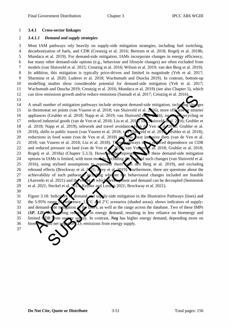
Final Government Distribution Chapter 3 IPCC AR6 WGIII
Do Not Cite, Quote or Distribute 3-51 Total pages: 156
3.4.1 Cross-sector linkages 1
3.4.1.1 Demand and supply strategies 2
Most IAM pathways rely heavily on supply-side mitigation strategies, including fuel switching, 3
decarbonization of fuels, and CDR (Creutzig et al. 2016; Bertram et al. 2018; Rogelj et al. 2018b; 4
Mundaca et al. 2019). For demand-side mitigation, IAMs incorporate changes in energy efficiency, 5
but many other demand-side options (e.g., behaviour and lifestyle changes) are often excluded from 6
models (van Sluisveld et al. 2015; Creutzig et al. 2016; Wilson et al. 2019; van den Berg et al. 2019). 7
In addition, this mitigation is typically price-driven and limited in magnitude (Yeh et al. 2017; 8
Sharmina et al. 2020; Luderer et al. 2018; Wachsmuth and Duscha 2019). In contrast, bottom-up 9
modelling studies show considerable potential for demand-side mitigation (Yeh et al. 2017; 10
Wachsmuth and Duscha 2019; Creutzig et al. 2016; Mundaca et al. 2019) (see also Chapter 5), which 11
can slow emissions growth and/or reduce emissions (Samadi et al. 2017; Creutzig et al. 2016). 12
13
A small number of mitigation pathways include stringent demand-side mitigation, including changes 14
in thermostat set points (van Vuuren et al. 2018; van Sluisveld et al. 2016), more efficient or smarter 15
appliances (Grubler et al. 2018; Napp et al. 2019; van Sluisveld et al. 2016), increased recycling or 16
reduced industrial goods (van de Ven et al. 2018; Liu et al. 2018; van Sluisveld et al. 2016; Grubler et 17
al. 2018; Napp et al. 2019), telework and travel avoidance (van de Ven et al. 2018; Grubler et al. 18
2018), shifts to public transit (van Vuuren et al. 2018; van Sluisveld et al. 2016; Grubler et al. 2018), 19
reductions in food waste (van de Ven et al. 2018) and less meat intensive diets (van de Ven et al. 20
2018; van Vuuren et al. 2018; Liu et al. 2018). These pathways show reduced dependence on CDR 21
and reduced pressure on land (van de Ven et al. 2018; van Vuuren et al. 2018; Grubler et al. 2018; 22
Rogelj et al. 2018a) (Chapter 5.3.3). However, the representation of these demand-side mitigation 23
options in IAMs is limited, with most models excluding the costs of such changes (van Sluisveld et al. 24
2016), using stylised assumptions to represent them (van den Berg et al. 2019), and excluding 25
rebound effects (Brockway et al. 2021; Krey et al. 2019). Furthermore, there are questions about the 26
achievability of such pathways, including whether the behavioural changes included are feasible 27
(Azevedo et al. 2021) and the extent to which development and demand can be decoupled (Semieniuk 28
et al. 2021; Steckel et al. 2013; Keyßer and Lenzen 2021; Brockway et al. 2021). 29
30
Figure 3.18: Indicators of demand and supply-side mitigation in the Illustrative Pathways (lines) and 31
the 5-95% range of Reference, 1.5C and 2C scenarios (shaded areas). shows indicators of supply- 32
and demand-side mitigation in the IMPs, as well as the range across the database. Two of these IMPs 33
(SP, LD) show strong reductions in energy demand, resulting in less reliance on bioenergy and 34
limited CDR from energy supply. In contrast, Neg has higher energy demand, depending more on 35
bioenergy and net negative CO2 emissions from energy supply. 36
37 ACCEPTED VERSION
SUBJECT TO FIN
AL EDITS
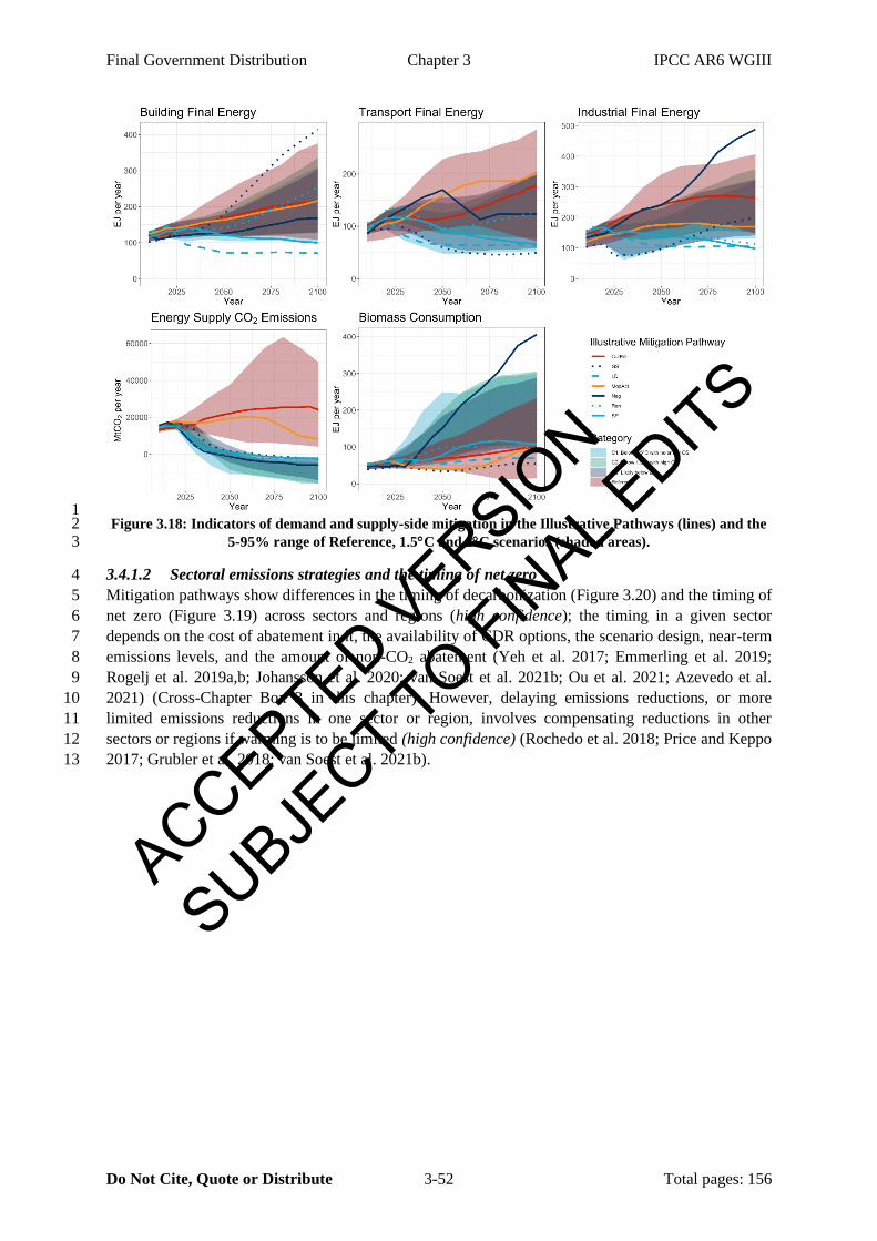
Final Government Distribution Chapter 3 IPCC AR6 WGIII
Do Not Cite, Quote or Distribute 3-52 Total pages: 156
1 Figure 3.18: Indicators of demand and supply-side mitigation in the Illustrative Pathways (lines) and the 2
5-95% range of Reference, 1.5C and 2C scenarios (shaded areas). 3
3.4.1.2 Sectoral emissions strategies and the timing of net zero 4
Mitigation pathways show differences in the timing of decarbonization (Figure 3.20) and the timing of 5
net zero (Figure 3.19) across sectors and regions (high confidence); the timing in a given sector 6
depends on the cost of abatement in it, the availability of CDR options, the scenario design, near-term 7
emissions levels, and the amount of non-CO2 abatement (Yeh et al. 2017; Emmerling et al. 2019; 8
Rogelj et al. 2019a,b; Johansson et al. 2020; van Soest et al. 2021b; Ou et al. 2021; Azevedo et al. 9
2021) (Cross-Chapter Box 3 in this chapter). However, delaying emissions reductions, or more 10
limited emissions reductions in one sector or region, involves compensating reductions in other 11
sectors or regions if warming is to be limited (high confidence) (Rochedo et al. 2018; Price and Keppo 12
2017; Grubler et al. 2018; van Soest et al. 2021b). 13
ACCEPTED VERSION
SUBJECT TO FIN
AL EDITS

Final Government Distribution Chapter 3 IPCC AR6 WGIII
Do Not Cite, Quote or Distribute 3-53 Total pages: 156
Table 3.4: Energy, emissions and CDR characteristics of the pathways by climate category for 2030, 2050, 2100. Source: AR6 scenarios database 1
2 Footnotes
0 Values in the table refer to the 50th and (5th-95th) percentile values.
1 Category definitions consider at peak warming and warming at the end-of-century (2100).
C1: Below 1.5°C in 2100 with a greater than 50% probability and a peak warming higher than 1.5°C with less than 67% probability.
C2: Below 1.5°C in 2100 with a greater than 50% probability but peak warming higher than 1.5°C with greater than or equal to 67% probability.
C3: Likely below 2 °C throughout the century with greater than 67% probability.
C4, C5, C6, C7: Below 2 °C, 2.5 °C, 3 °C and 4 °C throughout the century, respectively, with greater than 50% probability.
C8: Peak warming above 4 °C with greater than or equal to 50% probability. 2 The warming profile of Neg peaks around 2060 and declines thereafter to below 1.5°C (50% likelihood) shortly after 2100. Whilst technically classified as a C3, it
strongly exhibits the characteristics of C2 high overshoot scenarios. 3 Primary Energy as calculated in 'Direct Equivalent' terms according to IPCC reporting conventions.
4 Low carbon energy here defined to include: renewables (including biomass, solar, wind, hydro, geothermal, ocean); fossil fuels when used with CCS; and, nuclear power.
ACCEPTED VERSION
SUBJECT TO FIN
AL EDITS
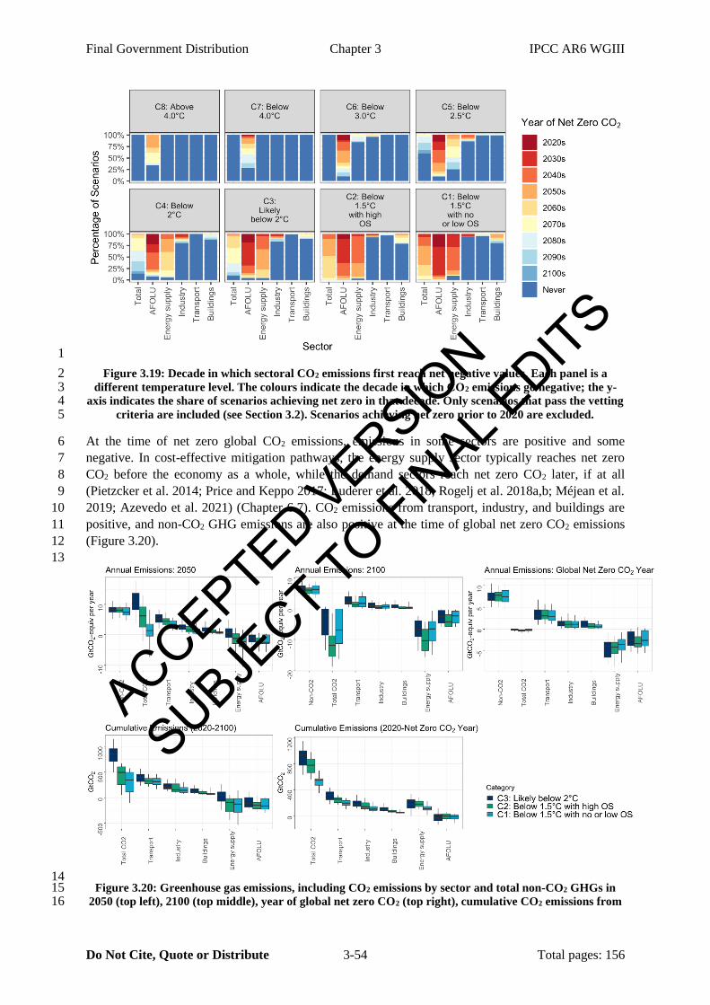
Final Government Distribution Chapter 3 IPCC AR6 WGIII
Do Not Cite, Quote or Distribute 3-54 Total pages: 156
1
Figure 3.19: Decade in which sectoral CO2 emissions first reach net negative values. Each panel is a 2 different temperature level. The colours indicate the decade in which CO2 emissions go negative; the y-3
axis indicates the share of scenarios achieving net zero in that decade. Only scenarios that pass the vetting 4 criteria are included (see Section 3.2). Scenarios achieving net zero prior to 2020 are excluded. 5
At the time of net zero global CO2 emissions, emissions in some sectors are positive and some 6
negative. In cost-effective mitigation pathways, the energy supply sector typically reaches net zero 7
CO2 before the economy as a whole, while the demand sectors reach net zero CO2 later, if at all 8
(Pietzcker et al. 2014; Price and Keppo 2017; Luderer et al. 2018; Rogelj et al. 2018a,b; Méjean et al. 9
2019; Azevedo et al. 2021) (Chapter 6.7). CO2 emissions from transport, industry, and buildings are 10
positive, and non-CO2 GHG emissions are also positive at the time of global net zero CO2 emissions 11
(Figure 3.20). 12
13
14 Figure 3.20: Greenhouse gas emissions, including CO2 emissions by sector and total non-CO2 GHGs in 15
2050 (top left), 2100 (top middle), year of global net zero CO2 (top right), cumulative CO2 emissions from 16
ACCEPTED VERSION
SUBJECT TO FIN
AL EDITS
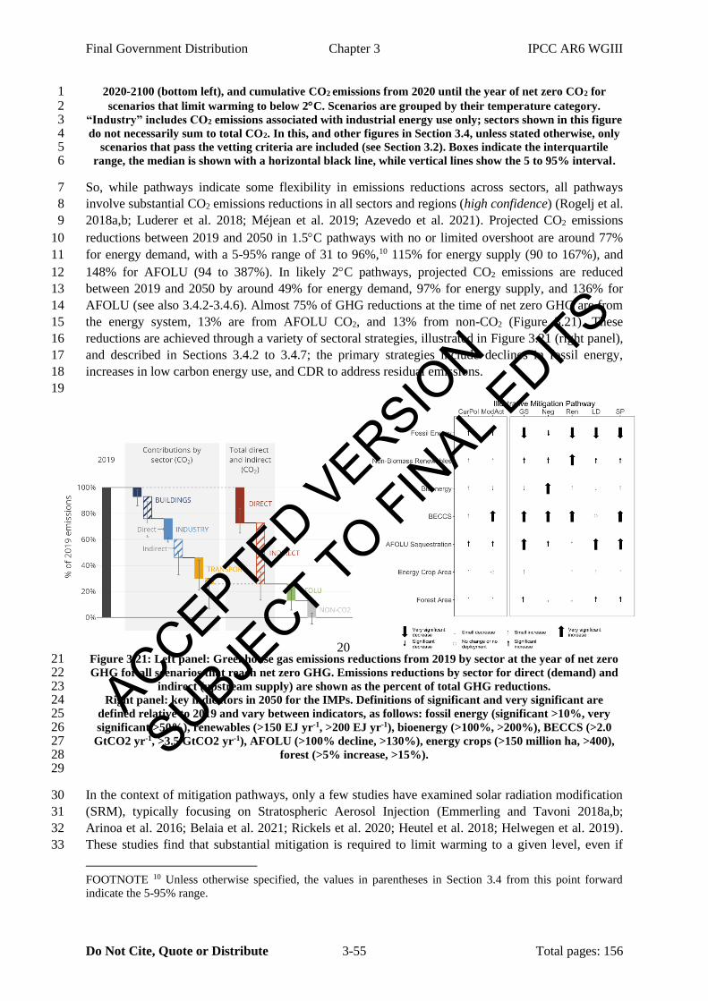
Final Government Distribution Chapter 3 IPCC AR6 WGIII
Do Not Cite, Quote or Distribute 3-55 Total pages: 156
2020-2100 (bottom left), and cumulative CO2 emissions from 2020 until the year of net zero CO2 for 1 scenarios that limit warming to below 2C. Scenarios are grouped by their temperature category. 2
“Industry” includes CO2 emissions associated with industrial energy use only; sectors shown in this figure 3 do not necessarily sum to total CO2. In this, and other figures in Section 3.4, unless stated otherwise, only 4
scenarios that pass the vetting criteria are included (see Section 3.2). Boxes indicate the interquartile 5 range, the median is shown with a horizontal black line, while vertical lines show the 5 to 95% interval. 6
So, while pathways indicate some flexibility in emissions reductions across sectors, all pathways 7
involve substantial CO2 emissions reductions in all sectors and regions (high confidence) (Rogelj et al. 8
2018a,b; Luderer et al. 2018; Méjean et al. 2019; Azevedo et al. 2021). Projected CO2 emissions 9
reductions between 2019 and 2050 in 1.5C pathways with no or limited overshoot are around 77% 10
for energy demand, with a 5-95% range of 31 to 96%,10 115% for energy supply (90 to 167%), and 11
148% for AFOLU (94 to 387%). In likely 2C pathways, projected CO2 emissions are reduced 12
between 2019 and 2050 by around 49% for energy demand, 97% for energy supply, and 136% for 13
AFOLU (see also 3.4.2-3.4.6). Almost 75% of GHG reductions at the time of net zero GHG are from 14
the energy system, 13% are from AFOLU CO2, and 13% from non-CO2 (Figure 3.21). These 15
reductions are achieved through a variety of sectoral strategies, illustrated in Figure 3.21 (right panel), 16
and described in Sections 3.4.2 to 3.4.7; the primary strategies include declines in fossil energy, 17
increases in low carbon energy use, and CDR to address residual emissions. 18
19
20 Figure 3.21: Left panel: Greenhouse gas emissions reductions from 2019 by sector at the year of net zero 21 GHG for all scenarios that reach net zero GHG. Emissions reductions by sector for direct (demand) and 22
indirect (upstream supply) are shown as the percent of total GHG reductions. 23 Right panel: key indicators in 2050 for the IMPs. Definitions of significant and very significant are 24
defined relative to 2019 and vary between indicators, as follows: fossil energy (significant >10%, very 25 significant >50%), renewables (>150 EJ yr-1, >200 EJ yr-1), bioenergy (>100%, >200%), BECCS (>2.0 26
GtCO2 yr-1, >3.5 GtCO2 yr-1), AFOLU (>100% decline, >130%), energy crops (>150 million ha, >400), 27 forest (>5% increase, >15%). 28
29
In the context of mitigation pathways, only a few studies have examined solar radiation modification 30
(SRM), typically focusing on Stratospheric Aerosol Injection (Emmerling and Tavoni 2018a,b; 31
Arinoa et al. 2016; Belaia et al. 2021; Rickels et al. 2020; Heutel et al. 2018; Helwegen et al. 2019). 32
These studies find that substantial mitigation is required to limit warming to a given level, even if 33
FOOTNOTE 10 Unless otherwise specified, the values in parentheses in Section 3.4 from this point forward
indicate the 5-95% range.
ACCEPTED VERSION
SUBJECT TO FIN
AL EDITS

Final Government Distribution Chapter 3 IPCC AR6 WGIII
Do Not Cite, Quote or Distribute 3-56 Total pages: 156
SRM is available (Moreno-Cruz and Smulders 2017; Emmerling and Tavoni 2018b; Belaia et al. 1
2021). SRM may reduce some climate impacts, reduce peak temperatures, lower mitigation costs, and 2
extend the time available to achieve mitigation; however, SRM does not address ocean acidification 3
and may involve risks to crop yields, economies, human health, or ecosystems (WGII Chapter 16; 4
WGI TS; WGI Ch 5; SR1.5 SPM; Cross-Working Group Box 4 in Chapter 14). There also are 5
significant uncertainties surrounding SRM, including uncertainties on the costs and risks, which can 6
substantially alter the amount of SRM used in modelled pathways (Tavoni et al. 2017; NASEM 2021; 7
Heutel et al. 2018; Helwegen et al. 2019; IPCC 2018). Furthermore, the degree of international 8
cooperation can influence the amount of SRM deployed in scenarios, with uncoordinated action 9
resulting in larger SRM deployment and consequently larger risks/impacts from SRM (Emmerling 10
and Tavoni 2018a). Bridging research and governance involves consideration of the full range of 11
societal choices and ramifications (Sugiyama et al. 2018). More information on SRM, including the 12
caveats, risks, uncertainties, and governance issues is found in WGI Chapter 4, WGIII Chapter 14, 13
and Cross-Working Group Box 4 in Chapter 14). 14
15
3.4.1.3 Linkages among sectors 16
Mitigation in one sector can be dependent upon mitigation in another sector, or may involve trade-offs 17
between sectors. Mitigation in energy demand often includes electrification (Luderer et al. 2018; 18
Pietzcker et al. 2014; Sharmina et al. 2020; DeAngelo et al. 2021), however such pathways only result 19
in reduced emissions if the electricity sector is decarbonized (Zhang and Fujimori 2020) (see also 20
Chapter 12). Relatedly, the mitigation potential of some sectors (e.g., transportation) depends on the 21
decarbonization of liquid fuels, e.g., through biofuels (Wise et al. 2017; Pietzcker et al. 2014; 22
Sharmina et al. 2020); Chapter 12). In other cases, mitigation in one sector results in reduced 23
emissions in another sector. For example, increased recycling can reduce primary resource extraction; 24
planting trees or green roofs in urban areas can reduce the energy demand associated with space 25
cooling (Chapter 12). 26
27
Mitigation in one sector can also result in additional emissions in another. One example is 28
electrification of end use which can result in increased emissions from energy supply. However, one 29
comparitively well-researched example of this linkage is bioenergy. An increase in demand for 30
bioenergy within the energy system has the potential to influence emissions in the AFOLU sector 31
through the intensification of land and forest management and/or via land use change (Smith et al. 32
2019; Daioglou et al. 2019; Smith et al. 2020a; IPCC 2019a). The effect of bioenergy and BECCS on 33
mitigation depends on a variety of factors in modelled pathways. In the energy system, the emissions 34
mitigation depends on the scale of deployment, the conversion technology, and the fuel displaced 35
(Calvin et al. 2021). Limiting or excluding bioenergy and/or BECCS increases mitigation cost and 36
may limit the ability of a model to reach a low warming level (Edmonds et al. 2013; Calvin et al. 37
2014b; Muratori et al. 2020; Luderer et al. 2018). In AFOLU, bioenergy can increase or decrease 38
terrestrial carbon stocks and carbon sequestration, depending on the scale, biomass feedstock, land 39
management practices, and prior land use (Calvin et al. 2014c; Wise et al. 2015; Smith et al. 2019, 40
2020a; IPCC 2019a; Calvin et al. 2021). 41
42
Pathways with very high biomass production for energy use typically include very high carbon prices 43
in the energy system (Popp et al. 2017; Rogelj et al. 2018b), little or no land policy (Calvin et al. 44
2014b), a high discount rate (Emmerling et al. 2019), and limited non-BECCS CDR options (e.g., 45
afforestation, DACCS) (Fuhrman et al. 2020; Realmonte et al. 2019; Chen and Tavoni 2013; 46
Marcucci et al. 2017; Calvin et al. 2014b). Higher levels of bioenergy consumption are likely to 47
involve trade-offs with mitigation in other sectors, notably in construction (i.e., wood for material and 48
structural products) and AFOLU (carbon stocks and future carbon sequestration), as well as trade-offs 49
with sustainability (Section 3.7) and feasibility concerns (Section 3.8). Not all of these trade-offs are 50
ACCEPTED VERSION
SUBJECT TO FIN
AL EDITS
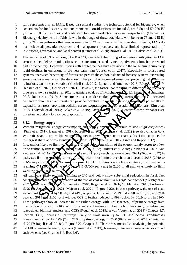
Final Government Distribution Chapter 3 IPCC AR6 WGIII
Do Not Cite, Quote or Distribute 3-57 Total pages: 156
fully represented in all IAMs. Based on sectoral studies, the technical potential for bioenergy, when 1
constraints for food security and environmental considerations are included, are 5-50 and 50-250 EJ 2
yr-1 in 2050 for residues and dedicated biomass production systems, respectively (Chapter 7). 3
Bioenergy deployment in IAMs is within the range of these potentials, with between 75 and 248 EJ 4
yr-1 in 2050 in pathways that limit warming to 1.5C with no or limited overshoot. Finally, IAMs do 5
not include all potential feedstock and management practices, and have limited representation of 6
institutions, governance, and local context (Butnar et al. 2020; Brown et al. 2019; Calvin et al. 2021). 7
The inclusion of CDR options, like BECCS, can affect the timing of emissions mitigation in IAM 8
scenarios, i.e., delays in mitigations actions are compensated by net negative emissions in the second 9
half of the century. However, studies with limited net negative emissions in the long-term require very 10
rapid declines in emissions in the near-term (van Vuuren et al. 2017). Especially in forest-based 11
systems, increased harvesting of forests can perturb the carbon balance of forestry systems, increasing 12
emissions for some period; the duration of this period of increased emissions, preceding net emissions 13
reductions, can be very variable (Mitchell et al. 2012; Lamers and Junginger 2013; Röder et al. 2019; 14
Hanssen et al. 2020; Cowie et al. 2021). However, the factors contributing to differences in recovery 15
time are known (Zanchi et al. 2012; Laganière et al. 2017; Mitchell et al. 2012; Lamers and Junginger 16
2013; Röder et al. 2019). Some studies that consider market-mediated effects find that an increased 17
demand for biomass from forests can provide incentives to maintain existing forests and potentially to 18
expand forest areas, providing addition carbon sequestration as well as additional biomass (Kim et al. 19
2018; Dwivedi et al. 2014; Baker et al. 2019; Favero et al. 2020). However, these responses are 20
uncertain and likely to vary geographically. 21
22
3.4.2 Energy supply 23
Without mitigation, energy consumption and supply emissions continue to rise (high confidence) 24
(Riahi et al. 2017; Bauer et al. 2017; Kriegler et al. 2016; Mcjeon et al. 2021) (see also Chapter 6.7). 25
While the share of renewable energy continues to grow in reference scenarios, fossil fuel accounts for 26
the largest share of primary energy (Riahi et al. 2017; Bauer et al. 2017; Price and Keppo 2017). 27
In scenarios likely to limit warming to 2℃ and below, transition of the energy supply sector to a low 28
or no carbon system is rapid (Rogelj et al. 2016, 2018b; Luderer et al. 2018; Grubler et al. 2018; van 29
Vuuren et al. 2018). CO2 emissions from energy supply reach net zero around 2041 (2033 to 2057) in 30
pathways limiting warming to below 1.5℃ with no or limited overshoot and around 2053 (2040 to 31
2066) in pathways likely to limit warming to 2℃. Emissions reductions continue, with emissions 32
reaching -7.1 GtCO2 per year (-15 to -2.3 GtCO2 per year) in 2100 in all pathways likely to limit 33
warming to 2℃ and below. 34
All pathways likely to limit warming to 2C and below show substantial reductions in fossil fuel 35
consumption and a near elimination of the use of coal without CCS (high confidence) (Welsby et al. 36
2021; Bauer et al. 2017; van Vuuren et al. 2018; Rogelj et al. 2018a,b; Grubler et al. 2018; Luderer et 37
al. 2018; Azevedo et al. 2021; Mcjeon et al. 2021) (Figure 3.22). In these pathways, the use of coal, 38
gas and oil is reduced by 90, 25, and 41%, respectively, between 2019 and 2050 and 91, 39, and 78% 39
between 2019 and 2100; coal without CCS is further reduced to 99% below its 2019 levels in 2100. 40
These pathways show an increase in low carbon energy, with 88% (69-97%) of primary energy from 41
low carbon sources in 2100, with different combinations of low carbon fuels (e.g., non-biomass 42
renewables, biomass, nuclear, and CCS) (Rogelj et al. 2018a,b; van Vuuren et al. 2018) (Chapter 6.7, 43
Section 3.4.1). Across all pathways likely to limit warming to 2℃ and below, non-biomass 44
renewables account for 52% (24 to 77%) of primary energy in 2100 (Pietzcker et al. 2017; Creutzig et 45
al. 2017; Rogelj et al. 2018b); Figure 3.22, Chapter 6). There are some studies analysing the potential 46
for 100% renewable energy systems (Hansen et al. 2019); however, there are a range of issues around 47
such systems (see Chapter 6.6, Box 6.6). 48
ACCEPTED VERSION
SUBJECT TO FIN
AL EDITS
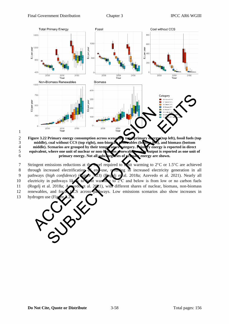
Final Government Distribution Chapter 3 IPCC AR6 WGIII
Do Not Cite, Quote or Distribute 3-58 Total pages: 156
1
Figure 3.22 Primary energy consumption across scenarios: total primary energy (top left), fossil fuels (top 2 middle), coal without CCS (top right), non-biomass renewables (bottom left), and biomass (bottom 3 middle). Scenarios are grouped by their temperature category. Primary energy is reported in direct 4
equivalent, where one unit of nuclear or non-biomass renewable energy output is reported as one unit of 5 primary energy. Not all subcategories of primary energy are shown. 6
Stringent emissions reductions at the level required to limit warming to 2C or 1.5C are achieved 7
through increased electrification of end-use, resulting in increased electricity generation in all 8
pathways (high confidence) (Figure 3.23) (Rogelj et al. 2018a; Azevedo et al. 2021). Nearly all 9
electricity in pathways likely to limit warming to 2℃ and below is from low or no carbon fuels 10
(Rogelj et al. 2018a; Azevedo et al. 2021), with different shares of nuclear, biomass, non-biomass 11
renewables, and fossil CCS across pathways. Low emissions scenarios also show increases in 12
hydrogen use (Figure 3.23). 13
ACCEPTED VERSION
SUBJECT TO FIN
AL EDITS
Final Government Distribution Chapter 3 IPCC AR6 WGIII
Do Not Cite, Quote or Distribute 3-59 Total pages: 156
1
Figure 3.23: Electricity (top left), share of low carbon electricity (top right), and hydrogen (bottom left) 2 production across all scenarios, grouped by the categories introduced in section 3.2. Low carbon includes 3
non-biomass renewables, biomass, nuclear, and CCS. 4
3.4.3 Buildings 5
Global final energy use in the building sector increases in all pathways as a result of population 6
growth and increasing affluence (Figure 3.24). There is very little difference in final energy intensity 7
for the buildings sector across scenarios. Direct CO2 emissions from the buildings sector vary more 8
widely across temperature stabilization levels than energy consumption. In 2100, scenarios above 3ºC 9
[C7-C8] still show an increase of CO2 emissions from buildings around 29% above 2019, while all 10
scenarios likely to limit warming to 2ºC and below have emission reductions of around 85% (8-11
100%). Carbon intensity declines in all scenarios, but much more sharply as the warming level is 12
reduced. 13
ACCEPTED VERSION
SUBJECT TO FIN
AL EDITS
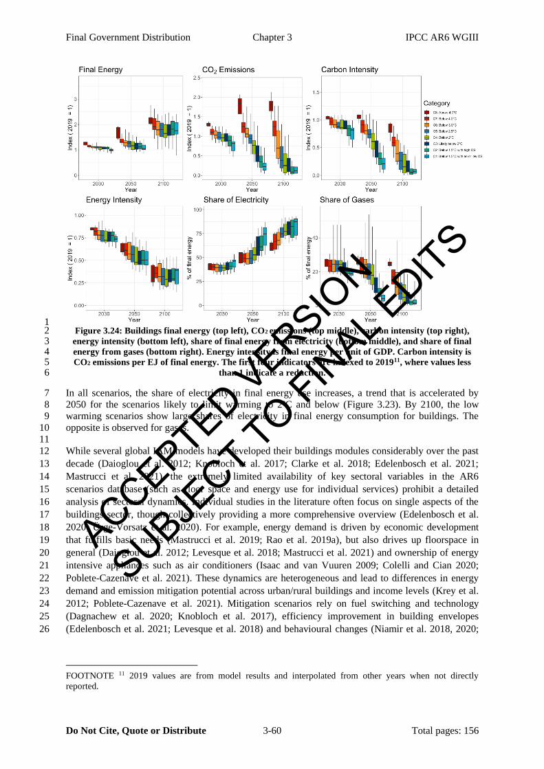
Final Government Distribution Chapter 3 IPCC AR6 WGIII
Do Not Cite, Quote or Distribute 3-60 Total pages: 156
1 Figure 3.24: Buildings final energy (top left), CO2 emissions (top middle), carbon intensity (top right), 2
energy intensity (bottom left), share of final energy from electricity (bottom middle), and share of final 3 energy from gases (bottom right). Energy intensity is final energy per unit of GDP. Carbon intensity is 4 CO2 emissions per EJ of final energy. The first four indicators are indexed to 201911, where values less 5
than 1 indicate a reduction. 6
In all scenarios, the share of electricity in final energy use increases, a trend that is accelerated by 7
2050 for the scenarios likely to limit warming to 2ºC and below (Figure 3.23). By 2100, the low 8
warming scenarios show large shares of electricity in final energy consumption for buildings. The 9
opposite is observed for gases. 10
11
While several global IAM models have developed their buildings modules considerably over the past 12
decade (Daioglou et al. 2012; Knobloch et al. 2017; Clarke et al. 2018; Edelenbosch et al. 2021; 13
Mastrucci et al. 2021), the extremely limited availability of key sectoral variables in the AR6 14
scenarios database (such as floor space and energy use for individual services) prohibit a detailed 15
analysis of sectoral dynamics. Individual studies in the literature often focus on single aspects of the 16
buildings sector, though collectively providing a more comprehensive overview (Edelenbosch et al. 17
2020; Ürge-Vorsatz et al. 2020). For example, energy demand is driven by economic development 18
that fulfills basic needs (Mastrucci et al. 2019; Rao et al. 2019a), but also drives up floorspace in 19
general (Daioglou et al. 2012; Levesque et al. 2018; Mastrucci et al. 2021) and ownership of energy 20
intensive appliances such as air conditioners (Isaac and van Vuuren 2009; Colelli and Cian 2020; 21
Poblete-Cazenave et al. 2021). These dynamics are heterogeneous and lead to differences in energy 22
demand and emission mitigation potential across urban/rural buildings and income levels (Krey et al. 23
2012; Poblete-Cazenave et al. 2021). Mitigation scenarios rely on fuel switching and technology 24
(Dagnachew et al. 2020; Knobloch et al. 2017), efficiency improvement in building envelopes 25
(Edelenbosch et al. 2021; Levesque et al. 2018) and behavioural changes (Niamir et al. 2018, 2020; 26
FOOTNOTE 11 2019 values are from model results and interpolated from other years when not directly
reported.
ACCEPTED VERSION
SUBJECT TO FIN
AL EDITS
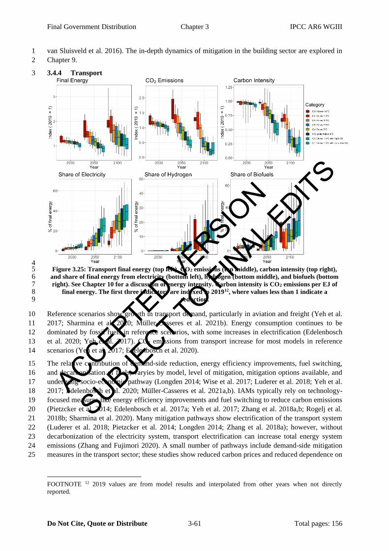
Final Government Distribution Chapter 3 IPCC AR6 WGIII
Do Not Cite, Quote or Distribute 3-61 Total pages: 156
van Sluisveld et al. 2016). The in-depth dynamics of mitigation in the building sector are explored in 1
Chapter 9. 2
3.4.4 Transport 3
4 Figure 3.25: Transport final energy (top left), CO2 emissions (top middle), carbon intensity (top right), 5
and share of final energy from electricity (bottom left), hydrogen (bottom middle), and biofuels (bottom 6 right). See Chapter 10 for a discussion of energy intensity. Carbon intensity is CO2 emissions per EJ of 7
final energy. The first three indicators are indexed to 201912, where values less than 1 indicate a 8 reduction. 9
Reference scenarios show growth in transport demand, particularly in aviation and freight (Yeh et al. 10
2017; Sharmina et al. 2020; Müller-Casseres et al. 2021b). Energy consumption continues to be 11
dominated by fossil fuels in reference scenarios, with some increases in electrification (Edelenbosch 12
et al. 2020; Yeh et al. 2017). CO2 emissions from transport increase for most models in reference 13
scenarios (Yeh et al. 2017; Edelenbosch et al. 2020). 14
The relative contribution of demand-side reduction, energy efficiency improvements, fuel switching, 15
and decarbonisation of fuels, varyies by model, level of mitigation, mitigation options available, and 16
underlying socio-economic pathway (Longden 2014; Wise et al. 2017; Luderer et al. 2018; Yeh et al. 17
2017; Edelenbosch et al. 2020; Müller-Casseres et al. 2021a,b). IAMs typically rely on technology-18
focused measures like energy efficiency improvements and fuel switching to reduce carbon emissions 19
(Pietzcker et al. 2014; Edelenbosch et al. 2017a; Yeh et al. 2017; Zhang et al. 2018a,b; Rogelj et al. 20
2018b; Sharmina et al. 2020). Many mitigation pathways show electrification of the transport system 21
(Luderer et al. 2018; Pietzcker et al. 2014; Longden 2014; Zhang et al. 2018a); however, without 22
decarbonization of the electricity system, transport electrification can increase total energy system 23
emissions (Zhang and Fujimori 2020). A small number of pathways include demand-side mitigation 24
measures in the transport sector; these studies show reduced carbon prices and reduced dependence on 25
FOOTNOTE 12 2019 values are from model results and interpolated from other years when not directly
reported.
ACCEPTED VERSION
SUBJECT TO FIN
AL EDITS
Final Government Distribution Chapter 3 IPCC AR6 WGIII
Do Not Cite, Quote or Distribute 3-62 Total pages: 156
CDR (Grubler et al. 2018; Méjean et al. 2019; van de Ven et al. 2018; Zhang et al. 2018c) (Section 1
3.4.1). 2
Across all IAM scenarios assessed, final energy demand for transport continues to grow, including in 3
many stringent mitigation pathways (Figure 3.25). The carbon intensity of energy declines 4
substantially by 2100 in likely 2°C and below scenarios, leading to substantial declines in transport 5
sector CO2 emissions with increased electrification of the transport system (Figure 3.23). 6
The transport sector has more detail than other sectors in many IAMs (Edelenbosch et al. 2020); 7
however, there is considerable variation across models. Some models (e.g., GCAM, IMAGE, 8
MESSAGE-GLOBIOM) represent different transport modes with endogenous shifts across modes as 9
a function of income, price, and modal speed (Edelenbosch et al. 2020).13 However, IAMs, including 10
those with detailed transport, exclude several supply-side (e.g., synthetic fuels) and demand-side (e.g., 11
behaviour change, reduced shipping, telework and automation) mitigation options (Davis et al. 2018; 12
Köhler et al. 2020; Mittal et al. 2017; Gota et al. 2019; Wilson et al. 2019; Creutzig et al. 2016; 13
Sharmina et al. 2020; Pietzcker et al. 2014; Lefèvre et al. 2021; Müller-Casseres et al. 2021a,b). 14
15
As a result of these missing options and differences in how mitigation is implemented, IAMs tend to 16
show less mitigation than the potential from national transport/energy models (Wachsmuth and 17
Duscha 2019; Gota et al. 2019; Yeh et al. 2017; Edelenbosch et al. 2020). For the transport sector as a 18
whole, studies suggest a mitigation potential of 4-5 GtCO2 per year in 2030 (Edelenbosch et al. 2020) 19
with complete decarbonization possible by 2050 (Gota et al. 2019; Wachsmuth and Duscha 2019). 20
However, in the scenarios assessed in this chapter that limit warming to below 1.5C with no or 21
limited overshoot, transport sector CO2 emissions are reduced by only 59% (28% to 81%) in 2050 22
compared to 2015. IAM pathways also show less electrification than the potential from other studies; 23
pathways that limit warming to below 1.5C with no or limited overshoot show a median of 25% (7 to 24
43%) of final energy from electricity in 2050, while the IEA NZE scenario includes 45% (IEA 25
2021a). 26
27
FOOTNOTE 13 Some of these models are treated as global transport energy sectoral models (GTEMs) in
Chapter 10.
ACCEPTED VERSION
SUBJECT TO FIN
AL EDITS

Final Government Distribution Chapter 3 IPCC AR6 WGIII
Do Not Cite, Quote or Distribute 3-63 Total pages: 156
3.4.5 Industry 1
2
Figure 3.26: Industrial final energy, including feedstocks (top left), CO2 emissions (top middle), carbon 3 intensity (top right), energy intensity (bottom left), share of final energy from electricity (bottom middle), 4
and share of final energy from gases (bottom right). Energy intensity is final energy per unit of GDP. 5 Carbon intensity is CO2 emissions per EJ of final energy. The first four indicators are indexed to 2019,14 6 where values less than 1 indicate a reduction. Industrial sector CO2 emissions include fuel combustion 7
emissions only. 8
Reference scenarios show declines in energy intensity, but increases in final energy use in the 9
industrial sector (Edelenbosch et al. 2017b). These scenarios show increases in CO2 emissions both 10
for the total industrial sector (Edelenbosch et al. 2020; Luderer et al. 2018; Edelenbosch et al. 2017b) 11
and individual subsectors like cement and iron and steel (van Ruijven et al. 2016; van Sluisveld et al. 12
2021) or chemicals (Daioglou et al. 2014; van Sluisveld et al. 2021). 13
In mitigation pathways, CO2 emissions reductions are achieved through a combination of energy 14
savings (via energy efficiency improvements and energy conservation), structural change, fuel 15
switching, and decarbonization of fuels (Grubler et al. 2018; Luderer et al. 2018; Edelenbosch et al. 16
2017b, 2020). Mitigation pathways show reductions in final energy for industry compared to the 17
baseline (Edelenbosch et al. 2017b; Luderer et al. 2018; Edelenbosch et al. 2020) and reductions in 18
the carbon intensity of the industrial sector through both fuel switching and the use of CCS (Paltsev et 19
al. 2021; Luderer et al. 2018; Edelenbosch et al. 2017b, 2020; van Ruijven et al. 2016; van Sluisveld 20
et al. 2021). The mitigation potential differs depending on the industrial subsector and the availability 21
of CCS, with larger potential reductions in the steel sector (van Ruijven et al. 2016) and cement 22
industry (Sanjuán et al. 2020) than in the chemicals sector (Daioglou et al. 2014). Many scenarios, 23
including stringent mitigation scenarios, show continued growth in final energy; however, the carbon 24
intensity of energy declines in all mitigation scenarios (Figure 3.26). 25
The representation of the industry sector is very aggregate in most IAMs, with only a small subset of 26
models disaggregating key sectors such as cement, fertilizer, chemicals, and iron and steel (Pauliuk et 27
FOOTNOTE 14 2019 values are from model results and interpolated from other years when not directly
reported.
ACCEPTED VERSION
SUBJECT TO FIN
AL EDITS

Final Government Distribution Chapter 3 IPCC AR6 WGIII
Do Not Cite, Quote or Distribute 3-64 Total pages: 156
al. 2017; Edelenbosch et al. 2017b; Daioglou et al. 2014; van Sluisveld et al. 2021) (Napp et al. 2019). 1
IAMs often account for both energy combustion and feedstocks (Edelenbosch et al. 2017b), but IAMs 2
typically ignore material flows and miss linkages between sectors (Kermeli et al. 2019; Pauliuk et al. 3
2017). By excluding these processes, IAMs misrepresent the mitigation potential of the industry 4
sector, e.g. by overlooking mitigation from material efficiency and circular economies (Sharmina et 5
al. 2020), which can have substantial mitigation potential (Chapter 5.3.4, Chapter 11.3). 6
Sectoral studies indicate a large mitigation potential in the industrial sector by 2050, including the 7
potential for net zero CO2 emissions for steel, plastics, ammonia, and cement (Section 11.4.1). 8
Detailed industry sector pathways show emissions reductions between 39 and 94% by mid-century 9
compared to present day15 (Section 11.4.2) and a substantial increase in direct electrification (IEA 10
2021a). IAMs show comparable mitigation potential to sectoral studies with median reductions in 11
CO2 emissions between 2019 and 2050 of 70% in scenarios likely to limit warming to 2C and below 12
and a maximum reduction of 96% (Figure 3.26). Some differences between IAMs and sectoral models 13
can be attributed to differences in technology availability, with IAMs sometimes including more 14
technologies (van Ruijven et al. 2016) and sometimes less (Sharmina et al. 2020). Figure 3.27: 15
Reduction in AFOLU GHG emissions from 2019. The AFOLU CO2 estimates in this figure are not 16
necessarily comparable with country GHG inventories (see Chapter 7). 17
3.4.6 Agriculture, Forestry and Other Land Use (AFOLU) 18
Mitigation pathways show substantial reductions in CO2 emissions, but more modest reductions in 19
AFOLU CH4 and N2O emissions (high confidence) (Popp et al. 2017; Roe et al. 2019; Reisinger et al. 20
2021) (Figure 3.27). Pathways limiting warming to likely 2C or below are projected to reach net zero 21
CO2 emissions in the AFOLU sector around 2033 (2024-2060); however AFOLU CH4 and N2O 22
emissions remain positive in all pathways (Figure 3.27). While IAMs include many land-based 23
mitigation options, these models exclude several options with large mitigation potential, such as 24
biochar, agroforestry, restoration/avoided conversion of coastal wetlands, and restoration/avoided 25
conversion of peatland (Smith et al. 2019; IPCC 2019a) (see also Chapter 7, Section 3.4). Sectoral 26
studies show higher mitigation potential than IAM pathways, as these studies include more mitigation 27
options than IAMs (medium confidence) (Chapter 7). 28
29
FOOTNOTE 15 Some studies calculate emissions reductions in 2050 compared to 2014, while others note
emissions reductions in 2060 relative to 2018.
ACCEPTED VERSION
SUBJECT TO FIN
AL EDITS

Final Government Distribution Chapter 3 IPCC AR6 WGIII
Do Not Cite, Quote or Distribute 3-65 Total pages: 156
1 Figure 3.27: Reduction in AFOLU GHG emissions from 2019. The AFOLU CO2 estimates in this figure 2
are not necessarily comparable with country GHG inventories (see Chapter 7). 3
Limiting warming to likely 2C or below can result in large scale transformation of the land surface 4
(high confidence) (Popp et al. 2017; Rogelj et al. 2018a,b; Brown et al. 2019; Roe et al. 2019). The 5
scale of land transformation depends, inter alia, on the temperature goal and the mitigation options 6
included (Popp et al. 2017; Rogelj et al. 2018a; IPCC 2019a). Pathways with more demand-side 7
mitigation options show less land transformation than those with more limited options (van Vuuren et 8
al. 2018; Grubler et al. 2018; IPCC 2019a). Most of these pathways show increases in forest cover, 9
with an increase of 322 million ha (-67 to 890 million ha) in 2050 in 1.5°C pathways with no or 10
limited overshoot, whereas bottom up models portray an economic potential of 300-500 million ha of 11
additional forest (Chapter 7). Many IAM pathways also include large amounts of energy cropland 12
area, to supply biomass for bioenergy and BECCS, with 199 (56-482) million ha in 2050 in 1.5°C 13
pathways with no or limited overshoot. Large land transformations, such as afforestation/reforestation 14
and widespread planting of energy crops, can have implications for biodiversity and sustainable 15
development (see Section 3.7, Chapter 7 - Subsection 7.7.4, Chapter 12 - Section 12.5). 16
ACCEPTED VERSION
SUBJECT TO FIN
AL EDITS
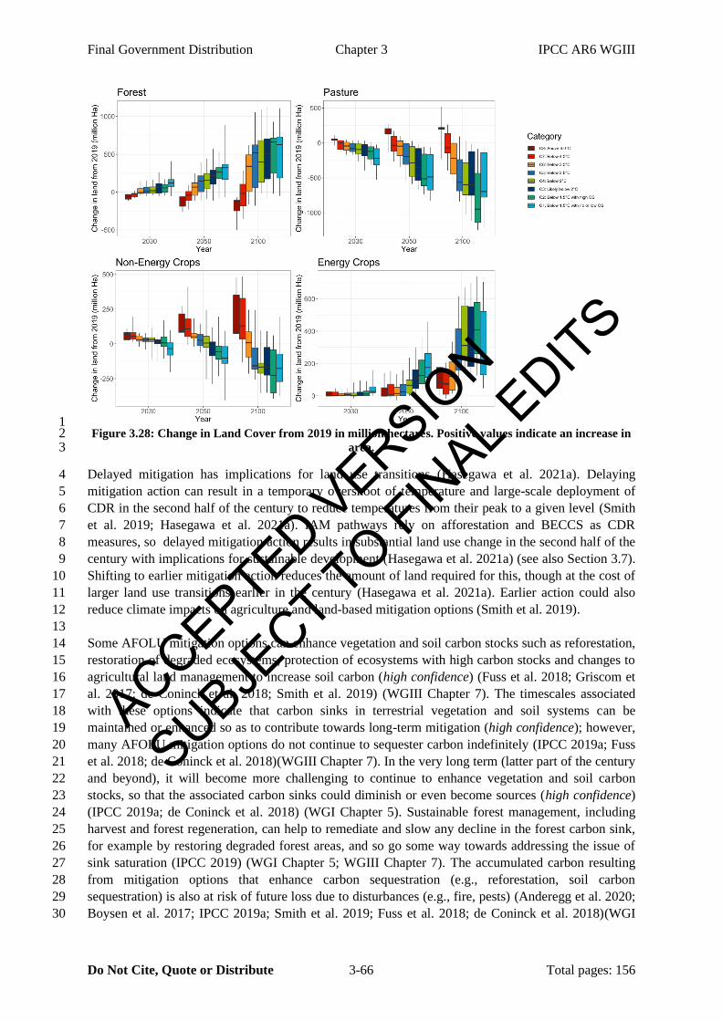
Final Government Distribution Chapter 3 IPCC AR6 WGIII
Do Not Cite, Quote or Distribute 3-66 Total pages: 156
1 Figure 3.28: Change in Land Cover from 2019 in million hectares. Positive values indicate an increase in 2
area. 3
Delayed mitigation has implications for land use transitions (Hasegawa et al. 2021a). Delaying 4
mitigation action can result in a temporary overshoot of temperature and large-scale deployment of 5
CDR in the second half of the century to reduce temperatures from their peak to a given level (Smith 6
et al. 2019; Hasegawa et al. 2021a). IAM pathways rely on afforestation and BECCS as CDR 7
measures, so delayed mitigation action results in substantial land use change in the second half of the 8
century with implications for sustainable development (Hasegawa et al. 2021a) (see also Section 3.7). 9
Shifting to earlier mitigation action reduces the amount of land required for this, though at the cost of 10
larger land use transitions earlier in the century (Hasegawa et al. 2021a). Earlier action could also 11
reduce climate impacts on agriculture and land-based mitigation options (Smith et al. 2019). 12
13
Some AFOLU mitigation options can enhance vegetation and soil carbon stocks such as reforestation, 14
restoration of degraded ecosystems, protection of ecosystems with high carbon stocks and changes to 15
agricultural land management to increase soil carbon (high confidence) (Fuss et al. 2018; Griscom et 16
al. 2017; de Coninck et al. 2018; Smith et al. 2019) (WGIII Chapter 7). The timescales associated 17
with these options indicate that carbon sinks in terrestrial vegetation and soil systems can be 18
maintained or enhanced so as to contribute towards long-term mitigation (high confidence); however, 19
many AFOLU mitigation options do not continue to sequester carbon indefinitely (IPCC 2019a; Fuss 20
et al. 2018; de Coninck et al. 2018)(WGIII Chapter 7). In the very long term (latter part of the century 21
and beyond), it will become more challenging to continue to enhance vegetation and soil carbon 22
stocks, so that the associated carbon sinks could diminish or even become sources (high confidence) 23
(IPCC 2019a; de Coninck et al. 2018) (WGI Chapter 5). Sustainable forest management, including 24
harvest and forest regeneration, can help to remediate and slow any decline in the forest carbon sink, 25
for example by restoring degraded forest areas, and so go some way towards addressing the issue of 26
sink saturation (IPCC 2019) (WGI Chapter 5; WGIII Chapter 7). The accumulated carbon resulting 27
from mitigation options that enhance carbon sequestration (e.g., reforestation, soil carbon 28
sequestration) is also at risk of future loss due to disturbances (e.g., fire, pests) (Anderegg et al. 2020; 29
Boysen et al. 2017; IPCC 2019a; Smith et al. 2019; Fuss et al. 2018; de Coninck et al. 2018)(WGI 30
ACCEPTED VERSION
SUBJECT TO FIN
AL EDITS
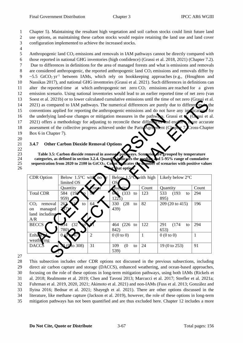
Final Government Distribution Chapter 3 IPCC AR6 WGIII
Do Not Cite, Quote or Distribute 3-67 Total pages: 156
Chapter 5). Maintaining the resultant high vegetation and soil carbon stocks could limit future land 1
use options, as maintaining these carbon stocks would require retaining the land use and land cover 2
configuration implemented to achieve the increased stocks. 3
4
Anthropogenic land CO2 emissions and removals in IAM pathways cannot be directly compared with 5
those reported in national GHG inventories (high confidence) (Grassi et al. 2018, 2021) (Chapter 7.2). 6
Due to differences in definitions for the area of managed forests and what is emissions and removals 7
are considered anthropogenic, the reported anthropogenic land CO2 emissions and removals differ by 8
~5.5 GtCO2 yr-1 between IAMs, which rely on bookkeeping approaches (e.g., (Houghton and 9
Nassikas 2017), and national GHG inventories (Grassi et al. 2021). Such differences in definitions can 10
alter the reported time at which anthropogenic net zero CO2 emissions are reached for a given 11
emission scenario. Using national inventories would lead to an earlier reported time of net zero (van 12
Soest et al. 2021b) or to lower calculated cumulative emissions until the time of net zero (Grassi et al. 13
2021) as compared to IAM pathways. The numerical differences are purely due to differences in the 14
conventions applied for reporting the anthropogenic emissions and do not have any implications for 15
the underlying land-use changes or mitigation measures in the pathways. Grassi et al. (Grassi et al. 16
2021) offers a methodology for adjusting to reconcile these differences and enable a more accurate 17
assessment of the collective progress achieved under the Paris Agreement (Chapter 7, Cross-Chapter 18
Box 6 in Chapter 7). 19
20
3.4.7 Other Carbon Dioxide Removal Options 21
22 Table 3.5: Carbon dioxide removal in assessed pathways. Scenarios are grouped by temperature 23
categories, as defined in section 3.2.4. Quantity indicates the median and 5-95% range of cumulative 24 sequestration from 2020 to 2100 in GtCO2. Count indicates the number of scenarios with positive values 25
for that option. 26
CDR Option Below 1.5°C with no or
limited OS
Below 1.5°C with high
OS
Likely below 2°C
Quantity Count Quantity Count Quantity Count
Total CDR 584 (192 to
959)
95 645 (333 to
1221)
123 533 (193 to
895)
294
CO2 removal
on managed
land including
A/R
262 (17 to
397)
64 330 (28 to
439)
82 209 (20 to 415) 196
BECCS 334 (32 to
780)
91 464 (226 to
842)
122 291 (174 to
653)
294
Enhanced
weathering
0 (0 to 47) 2 0 (0 to 0) 1 0 (0 to 0) 1
DACCS 30 (0 to 308) 31 109 (0 to
539)
24 19 (0 to 253) 91
27
This subsection includes other CDR options not discussed in the previous subsections, including 28
direct air carbon capture and storage (DACCS), enhanced weathering, and ocean-based approaches, 29
focusing on the role of these options in long-term mitigation pathways, using both IAMs (Rickels et 30
al. 2018; Realmonte et al. 2019; Chen and Tavoni 2013; Marcucci et al. 2017; Strefler et al. 2021a; 31
Fuhrman et al. 2019, 2020, 2021; Akimoto et al. 2021) and non-IAMs (Fuss et al. 2013; González and 32
Ilyina 2016; Bednar et al. 2021; Shayegh et al. 2021). There are other options discussed in the 33
literature, like methane capture (Jackson et al. 2019), however, the role of these options in long-term 34
mitigation pathways has not been quantified and are thus excluded here. Chapter 12 includes a more 35
ACCEPTED VERSION
SUBJECT TO FIN
AL EDITS
Final Government Distribution Chapter 3 IPCC AR6 WGIII
Do Not Cite, Quote or Distribute 3-68 Total pages: 156
detailed description of the individual technologies, including their costs, potentials, financing, risks, 1
impacts, maturity and upscaling. 2
Very few studies and pathways include other CDR options (Table 3.5). Pathways with DACCS 3
include potentially large removal from DACCS (up to 37 GtCO2 yr-1 in 2100) in the second half of the 4
century (Realmonte et al. 2019; Marcucci et al. 2017; Chen and Tavoni 2013; Fuhrman et al. 2020, 5
2021; Shayegh et al. 2021; Akimoto et al. 2021) and reduced cost of mitigation (Bistline and Blanford 6
2021; Strefler et al. 2021a). At large scales, the use of DACCS has substantial implications for energy 7
use, emissions, land, and water; substituting DACCS for BECCS results in increased energy usage, 8
but reduced land use change and water withdrawals (Fuhrman et al., 2020, 2021; Chapter 12.3.2; 9
IPCC WGI Chapter 5). The level of deployment of DACCS is sensitive to the rate at which it can be 10
scaled up, the climate goal or carbon budget, the underlying socioeconomic scenario, the availability 11
of other decarbonization options, the cost of DACCS and other mitigation options, and the strength of 12
carbon cycle feedbacks (Honegger and Reiner 2018; Fuss et al. 2013; Fuhrman et al. 2021; Bistline 13
and Blanford 2021; Chen and Tavoni 2013; Strefler et al. 2021a; Fuhrman et al. 2020; Realmonte et 14
al. 2019) (IPCC WGI Chapter 5). Since DACCS consumes energy, its effectiveness depends on the 15
type of energy used; the use of fossil fuels would reduce its sequestration efficiency (Creutzig et al. 16
2019; Babacan et al. 2020; NASEM 2019). Studies with additional CDR options in addition to 17
DACCS (e.g., enhanced weathering, BECCS, afforestation, biochar, and soil carbon sequestration) 18
find that CO2 removal is spread across available options (Holz et al. 2018; Strefler et al. 2021a). 19
Similar to DACCS, the deployment of deep ocean storage depends on cost and the strength of carbon 20
cycle feedbacks (Rickels et al. 2018). 21
22
23
3.5 Interaction between near-, medium- and long-term action in 24
mitigation pathways 25
This section assesses the relationship between long-term climate goals and short- to medium-term 26
emissions reduction strategies based on the mitigation pathway literature. After an overview of this 27
relationship (3.5.1), it provides an assessment of what currently planned near-term action implies for 28
limiting warming to 1.5-2°C (3.5.2), and to what extent pathways with accelerated action beyond 29
current NDCs can improve the ability to keep long-term targets in reach (3.5.3). 30
The assessment in this section shows that if mitigation ambitions in current NDCs16 are followed until 31
2030, leading to estimated emissions of 47-57 GtCO2-eq in 203017 (Chapter 4.2.2), it is no longer 32
possible to stay below 1.5°C warming with no or limited overshoot (high confidence). Instead, it 33
would entail high overshoot (typically >0.1oC) and reliance on net negative CO2 emissions with 34
uncertain potential to return warming to 1.5°C by the end of the century. It would also strongly 35
increase mitigation challenges to likely limit warming to 2°C (high confidence). GHG emissions 36
FOOTNOTE 16 The term “current NDCs” used in this section and throughout the report refers to the most
recent nationally determined contributions submitted to the UNFCCC as well as those publicly announced with
sufficient detail on targets, but not yet submitted, up to 11 October 2021, and reflected in studies published up to
11 October 2021. In contrast, “original NDCs” refers to nationally determined contributions that were initially
submitted to the Paris Agreement by parties, largely reflecting the state of submissions until the year 2019. See
Chapter 4.2.
FOOTNOTE 17 In this section, the emissions range associated with current (or original) NDCs refer to the
combined emissions ranges from the two cases of implementing only the unconditional elements of current
NDCs (50-57 GtCO2-eq) and implementing both unconditional and conditional elements of current NDCs (47-
53 GtCO2-eq), if not specified otherwise.
ACCEPTED VERSION
SUBJECT TO FIN
AL EDITS

Final Government Distribution Chapter 3 IPCC AR6 WGIII
Do Not Cite, Quote or Distribute 3-69 Total pages: 156
reductions would need to abruptly increase after 2030 to an annual average rate of 1.3-2.1 GtCO2-eq 1
during the period 2030-2050, around 70% higher than in mitigation pathways assuming immediate 2
action18 to likely limit warming to 2°C. The higher post-2030 reduction rates would have to be 3
obtained in an environment of continued build-up of fossil fuel infrastructure and less development of 4
low carbon alternatives until 2030. A lock-in into fossil-fuel intensive production systems (carbon 5
lock-in) will increase the societal, economic and political strain of a rapid low-carbon transition after 6
2030 (high confidence). 7
The section builds on previous assessments in the IPCC’s Fifth Assessment Report (Clarke et al. 8
2014) and Special Report on 1.5°C Warming (Rogelj et al. 2018a). The literature assessed in these 9
two reports has focused on delayed action until 2030 in the context of limiting warming to 2°C (den 10
Elzen et al. 2010; van Vuuren and Riahi 2011; Kriegler et al. 2015; Luderer et al. 2013, 2016; Riahi et 11
al. 2015; Rogelj et al. 2013a) and 1.5°C (Strefler et al. 2018; Luderer et al. 2018; Rogelj et al. 2013b). 12
Here we provide an update of these assessments drawing on the most recent literature on global 13
mitigation pathways. New studies have focused, inter alia, on constraining near term developments by 14
peak warming limits (Rogelj et al. 2019b; Strefler et al. 2021b; Riahi et al. 2021) and updating 15
assumptions about near- and medium term emissions developments based on national plans and long-16
term strategies (Roelfsema et al. 2020) (Chapter 4.2). Several studies have explored new types of 17
pathways with accelerated action bridging between current policy plans and the goal of limiting 18
warming below 2°C (Kriegler et al. 2018a; van Soest et al. 2021a) and looked at hybrid international 19
policy regimes to phase in global collective action (Bauer et al. 2020). 20
21
3.5.1 Relationship between long-term climate goals and near- to medium-term emissions 22
reductions 23
The close link between cumulative CO2 emissions and warming has strong implications for the 24
relationship between near-, medium-, and long-term climate action to limit global warming. The AR6 25
WGI Assessment has estimated a remaining carbon budget of 500 (400) GtCO2 from the beginning of 26
2020 onwards for staying below 1.5°C with 50% (67%) likelihood, subject to additional uncertainties 27
about historic warming and the climate response and variations in warming from non-CO2 climate 28
forcers (Canadell and Monteiro 2019) (see also WGI Chapter 5, Section 5.5). For comparison, if 29
current CO2 emissions of more than 40 GtCO2 are keeping up until 2030, more than 400 GtCO2 will 30
be emitted during 2021–2030, already exhausting the remaining carbon budget for 1.5°C by 2030. 31
The relationship between warming limits and near term action is illustrated in Figure 3.29, using a set 32
of 1.5-2°C scenarios with different levels of near term action, overshoot and non-CO2 warming 33
contribution from a recent study (Riahi et al. 2021). In general, the more CO2 is emitted until 2030, 34
the less CO2 can be emitted thereafter to stay within a remaining carbon budget and below a warming 35
limit. Scenarios with immediate action to observe the warming limit give the longest time to exhaust 36
the associated remaining carbon budget and reach net zero CO2 emissions (light blue line in Figure 37
3.29, Cross-Chapter Box 3 in this chapter). In comparison, following projected NDC emissions until 38
2030 would imply a more pronounced drop in emissions from 2030 levels to net zero to make up for 39
the additional near-term emissions (orange lines in Figure 3.29). If such a drop does not occur, the 40
remaining carbon budget is exceeded and net negative CO2 emissions are required to return global 41
mean temperature below the warming limit (black lines in Figure 3.29) (Fuss et al. 2014; Clarke et al. 42
2014; Rogelj et al. 2018a). 43
FOOTNOTE 18 In this section, near term emissions outcomes are often compared to near term emissions in
mitigation pathways with immediate action towards a warming limit. These are defined as pathways that
immediately after imposing the warming limit turn to global mitigation action tapping into all least cost
abatement options available globally. These pathways are often called cost-effective or least-cost pathways in
the literature. The onset of immediate action is defined by scenario design and is typically chosen to be the first
time step after 2020 in immediate action scenarios assessed in this report.
ACCEPTED VERSION
SUBJECT TO FIN
AL EDITS

Final Government Distribution Chapter 3 IPCC AR6 WGIII
Do Not Cite, Quote or Distribute 3-70 Total pages: 156
The relationship between warming limits and near-term action is also affected by the warming 1
contribution of non-CO2 greenhouse gases and other short lived climate forcers (3.3, Working Group I 2
6.7). The estimated budget values for limiting warming to 1.5-2°C already assume stringent 3
reductions in non-CO2 greenhouse gases and non-CO2 climate forcing as found in 1.5-2°C pathways 4
(3.3, Cross-Working Group Box 1; Working Group I 5.5, Box 5.2). Further variations in non-CO2 5
warming observed across 1.5-2°C pathways can vary the median estimate for the remaining carbon 6
budget by 220 GtCO2 (Working Group I 5.5). In 1.5-2°C pathways, the non-CO2 warming 7
contribution differs strongly between the near-, medium and long term. Changes to the atmospheric 8
composition of short-lived climate forcers dominate the warming response in the near term (Working 9
Group I 6.7). CO2 reductions are combined with strong reductions in air pollutant emissions due to 10
rapid reduction in fossil fuel combustion and in some cases the assumption of stringent air quality 11
policies (Rao et al. 2017b; Smith et al. 2020c). As air pollutants exert a net cooling effect, their 12
reduction drives up non-CO2 warming in the near term, which can be attenuated by the simultaneous 13
reduction of methane and black carbon (Smith et al. 2020b; Shindell and Smith 2019) (Working 14
Group I 6.7). After 2030, the reduction in methane concentrations and associated reductions in 15
tropospheric ozone levels tend to dominate so that a peak and decline in non-CO2 forcing and non-16
CO2 induced warming can occur before net zero CO2 is reached (Figure 3.29) (Rogelj et al. 2018a) 17
The more stringent the reductions in methane and other short-lived warming agents like black carbon, 18
the lower this peak and the earlier the decline of non-CO2 warming, leading to a reduction of warming 19
rates and overall warming in the near to medium term (Smith et al. 2020b; Harmsen et al. 2020). This 20
is important for keeping warming below a tight warming limit that is already reached around mid-21
century as is the case in 1.5°C pathways (Xu and Ramanathan 2017). Early and deep reductions of 22
methane emissions, and other short-lived warming agents like black carbon, provide space for residual 23
CO2-induced warming until the point of net zero CO2 emissions is reached (purple lines in Figure 24
3.29). Such emissions reductions have also been advocated due to co-benefits for, e.g., reducing air 25
pollution (Rao et al. 2016; Shindell et al. 2017a, 2018; Shindell and Smith 2019; Rauner et al. 2020a; 26
Vandyck et al. 2020). 27
ACCEPTED VERSION
SUBJECT TO FIN
AL EDITS

Final Government Distribution Chapter 3 IPCC AR6 WGIII
Do Not Cite, Quote or Distribute 3-71 Total pages: 156
1 Figure 3.29: Illustration of emissions and climate response in four mitigation pathways with different 2
assumptions about near term policy developments, global warming limit and non-CO2 warming 3 contribution drawn from Riahi et al. (2021). Shown are (a) CO2 emissions trajectories, (b) cumulative 4
CO2 emissions, (c) effective non-CO2 radiative forcing, and (d) the resulting estimate of the 67th percentile 5 of global mean temperature response relative to 1850-1900. Light blue lines show a scenario that acts 6
immediately on a remaining carbon budget of 900 GtCO2 from 2020 without allowing net negative CO2 7 emissions, i.e., temporary budget overshoot (COFFEE 1.1, Scenario EN_NPi2020_900). Orange and black 8
lines show scenarios drawn from the same model that follow the NDCs until 2030 and thereafter 9 introduce action to stay within the same budget – in one case excluding net negative CO2 emissions like 10
before (orange lines; COFFEE 1.1., Scenario EN-INDCi2030_900) and in the other allowing for a 11 temporary overshoot of the carbon budget until 2100 (black lines; COFFEE 1.1., Scenario EN-12
INDCi2030_900f). Light blue lines describe a scenario following the NDCs until 2030, and then aiming for 13 a higher budget of 2300 GtCO2 without overshoot (AIM/CGE 2.2, Scenario EN-INDCi2030_1200). It is 14
drawn from another model which projects a lower anthropogenic non-CO2 forcing contribution and 15 therefore achieves about the same temperature outcome as the other two non-overshoot scenarios despite 16 the higher CO2 budget. Grey funnels include the trajectories from all scenarios that likely limit warming 17
to 2°C (Category C3). Historical CO2 emissions until 2019 are from Chapter SM.2.1 EDGAR v6.0. 18
The relationship between long-term climate goals and near term action is further constrained by 19
social, technological, economic and political factors (Aghion et al. 2019; Mercure et al. 2019; van 20
Sluisveld et al. 2018b; Cherp et al. 2018; Jewell and Cherp 2020; Trutnevyte et al. 2019b). These 21
factors influence path dependency and transition speed (Vogt-Schilb et al. 2018; Pahle et al. 2018). 22
While detailed integrated assessment modelling of global mitigation pathways accounts for 23
technology inertia (Bertram et al. 2015a; Mercure et al. 2018) and technology innovation and 24
diffusion (Wilson et al. 2013; van Sluisveld et al. 2018a; Luderer et al. 2021), there are limitations in 25
capturing socio-technical and political drivers of innovation, diffusion and transition processes 26
(Keppo et al. 2021; Gambhir et al. 2019; Hirt et al. 2020; Köhler et al. 2019). Mitigation pathways 27
show a wide range of transition speeds that have been interrogated in the context of socio-technical 28
ACCEPTED VERSION
SUBJECT TO FIN
AL EDITS

Final Government Distribution Chapter 3 IPCC AR6 WGIII
Do Not Cite, Quote or Distribute 3-72 Total pages: 156
inertia (Gambhir et al. 2017; Kefford et al. 2018; Kriegler et al. 2018a; Brutschin et al. 2021) vs. 1
accelerating technological change and self-enforcing socio-economic developments (Creutzig et al. 2
2017; Zenghelis 2019) (Section 3.8). Diagnostic analysis of detailed IAMs found a lag of 8-20 years 3
between the convergence of emissions pricing and the convergence of emissions response after a 4
period of differentiated emission prices (Harmsen et al. 2021). This provides a measure of the inertia 5
to changing policy signals in the model response. It is about half the timescale of 20-40 years 6
observed for major energy transitions (Grubb et al. 2021). Hence, the mitigation pathways assessed 7
here capture socio-technical inertia in reducing emissions, but the limited modelling of socio-political 8
factors may alter the extent and persistence of this inertia. 9
10
3.5.2 Implications of near-term emission levels for keeping long-term climate goals within 11
reach 12
The implications of near-term climate action for long-term climate outcomes can be explored by 13
comparing mitigation pathways with different near-term emissions developments aiming for the same 14
climate target (Vrontisi et al. 2018; Riahi et al. 2015; Roelfsema et al. 2020). A particular example is 15
the comparison of cost-effective pathways with immediate action to limit warming to 1.5-2°C with 16
mitigation pathways pursuing more moderate mitigation action until 2030. After the adoption of the 17
Paris Agreement, near term action was often modelled to reflect conditional and unconditional 18
elements of originally submitted NDCs (2015-2019) (Fawcett et al. 2015; Fujimori et al. 2016a; 19
Kriegler et al. 2018a; Vrontisi et al. 2018; Roelfsema et al. 2020). The most recent modelling studies 20
also include submission of updated NDCs or announcements of planned updates in the first half of 21
2021 (Network for Greening the Financial System 2021; Riahi et al. 2021). Emissions levels under 22
current NDCs (see footnote 15) are assessed to range between 47–57 GtCO2-eq in 2030 (Chapter 23
4.2.2). This assessed range corresponds well to 2030 emissions levels in 2°C mitigation pathways in 24
the literature that are designed to follow the original or current NDCs until 203019. For the 139 25
scenarios of this kind that are collected in the AR6 scenario database and that still likely limit 26
warming to 2°C, the 2030 emissions range is 52.5 (44.5-57) GtCO2-eq (based on native model 27
reporting) and 52 (46.5-56) GtCO2-eq, respectively (based on harmonized emissions data for climate 28
assessment (Annex III part II section 2.4); median and 5th to 95th percentile). This close match allows 29
a robust assessment of the implications of implementing current NDCs for post-2030 mitigation 30
efforts and warming outcomes based on the literature and the AR6 scenarios database. 31
The assessed emission ranges from implementing the unconditional (unconditional and conditional) 32
elements of current NDCs implies an emissions gap to cost-effective mitigation pathways of 20-26 33
(16-24) GtCO2-eq in 2030 for limiting warming to 1.5°C with no or limited overshoot and 10-17 (7-34
14) GtCO2-eq in 2030 for likely limiting warming to 2°C (Chapter 4, Cross-Chapter Box 2 in chapter 35
2). The emissions gap gives rise to a number of mitigation challenges (Rogelj et al. 2013a; Kriegler et 36
al. 2013a, 2018b,a; Riahi et al. 2015; Luderer et al. 2013, 2018; Fujimori et al. 2016b; Fawcett et al. 37
2015; Strefler et al. 2018; Winning et al. 2019; UNEP 2020; SEI et al. 2020): (i) larger transitional 38
challenges post-2030 to still remain under the warming limit (, in particular higher CO2 emissions 39
reduction rates and technology transition rates required during 2030-2050; (ii) larger lock-in into 40
carbon-intensive infrastructure and increased risk of stranded fossil fuel assets (3.5.2.2); and (iii) 41
larger reliance on CDR to reach net zero CO2 more rapidly and compensate excess emissions in the 42
second half of the century (3.5.2.1). All these factors exacerbate socio-economic strain of 43
FOOTNOTE 19 The intended design of mitigation pathways in the literature can be deduced from underlying
publications and study protocols. This information was collected as part of this assessment to establish a
categorization of policy assumptions underpinning the mitigation pathways collected in the AR6 scenario
database (3.2; Annex III Part II section 3.2).
ACCEPTED VERSION
SUBJECT TO FIN
AL EDITS
Final Government Distribution Chapter 3 IPCC AR6 WGIII
Do Not Cite, Quote or Distribute 3-73 Total pages: 156
implementing the transition, leading to an increased risk of overshooting the warming and a higher 1
risk of climate change impacts (Drouet et al. 2021). 2
The challenges are illustrated in Table 3.6 and Figure 3.30, surveying global mitigation pathways in 3
the literature that were collected in the AR6 scenarios database. There is a clear trend of increasing 4
peak warming with increasing 2030 GHG emission levels (Figure 3.30a+b). In particular, there is no 5
mitigation pathway designed to follow the NDCs until 2030 in 2030 that can limit warming to 1.5°C 6
with no or limited overshoot. Our assessment confirms the finding of the IPCC Special Report on 7
1.5°C Warming for the case of current NDCs, including updates until 11 October 2021 that were 8
assessed in the literature, that pathways following the NDCs until 2030 “would not limit global 9
warming to 1.5°C, even if supplemented by very challenging increases in the scale and ambition of 10
emissions reductions after 2030” (SR1.5 SPM). This assessment is now more robust than in SR1.5 as 11
it is based on a larger set of 1.5-2°C pathways with better representation of current trends and plans 12
covering a wider range of post-2030 emissions developments. In particular, a recent multi-model 13
study limiting peak cumulative CO2 emissions for a wide range of carbon budgets and immediate vs 14
NDC-type action until 2030 established a feasibility frontier for the existence of such pathways across 15
participating models (Riahi et al. 2021). 16
2030 emissions levels in the NDC range also tighten the remaining space to likely limit warming 2°C. 17
As shown in Figure 3.30b, the 67th percentile of peak warming reaches values above 1.7°C warming 18
in pathways with 2030 emissions levels in this range. To still have a likely chance to stay below 2°C, 19
the global post-2030 GHG emission reduction rates would need to be abruptly raised in 2030 from 0-20
0.8 GtCO2-eq yr-1 to an average of 1.3-2.1 GtCO2-eq yr-1 during the period 2030-2050 (Figure 3.30c), 21
around 70% of that in immediate mitigation pathways confirming findings in the literature (Winning 22
et al. 2019). Their average reduction rate of 0.6-1.4 GtCO2 yr-1 would already be unprecedented at the 23
global scale and with a few exceptions national scale for an extended period of time (Riahi et al. 24
2015). For comparison, the impact of COVID-19 on the global economy is projected to lead to a 25
decline of ca. 2.5-3 GtCO2 of global CO2 emissions from fossil fuel and industry in 2020 26
(Friedlingstein et al. 2020) (Chapter 2.2). 27
The increased post-2030 transition challenge in mitigation pathways with moderate near term action is 28
also reflected in the timing of reaching net zero CO2 emissions (Figure 3.30d and Table 3.6) (Cross-29
Chapter Box 3 in this chapter). As 2030 emission levels and the cumulated CO2 emissions until 2030 30
increase, the remaining time for dropping to net zero CO2 and staying within the remaining carbon 31
budget shortens (Figure 3.29). This gives rise to an inverted v-shape of the lower bound on the year of 32
reaching net zero as a function of 2030 emissions levels. Reaching low in 2030 facilitates reaching net 33
zero early (left leg of the inverted v), but staying high until 2030 also requires to reach net zero CO2 34
faster to compensate for higher emissions early on (right leg of the inverted v). Overall, there is a 35
considerable spread of the timing of net zero CO2 for any 2030 emissions level due to variation in the 36
timing of spending the remaining carbon budget and the non-CO2 warming contribution (Cross-37
Chapter Box 3 in this chapter). 38
ACCEPTED VERSION
SUBJECT TO FIN
AL EDITS

Final Government Distribution Chapter 3 IPCC AR6 WGIII
Do Not Cite, Quote or Distribute 3-74 Total pages: 156
1 Figure 3.30: Relationship between level of global GHG emissions in 2030 and selected indicators as listed 2
in the panel titles for scenarios collected in the AR6 scenario database. Emissions data based on 3 harmonized emissions used for the climate assessment. All scenarios likely to limit warming to 2°C or 4
below are coloured blue or red (see p67 peak warming in panel b). The large majority of blue coloured 5 scenarios act immediately on the temperature target, while red coloured scenarios depict all those that 6 were designed to follow the NDCs or lesser action until 2030 and orange coloured scenarios comprise a 7 small set of pathways with additional regulatory action beyond NDCs (3.5.3). Grey coloured scenarios 8 exceed the 2°C (p67), either by temporary overshoot or towards the end of the century. Large markers 9
denote the 5 illustrative mitigation pathways (legend in Panel h; Section 3.2). Shaded yellow areas depict 10 the estimated range of 2030 emissions from current NDCs (Chapter 4.2.2). Dotted lines are inserted in 11 some panels to highlight trends in the dependency of selected output variables on 2030 GHG emissions 12
levels (see text) 13
There is also a profound impact on the underlying transition of energy and land use (Table 3.6 and 14
Figure 3.30f-h). Scenarios following NDCs until 2030 show a much smaller reduction in fossil fuel 15
use, only half of the growth in renewable energy use, and a smaller reduction in CO2 and CH4 land 16
use emissions in 2030 compared to immediate action scenarios. This is then followed by a much faster 17
reduction of land use emissions and fossil fuels, and a larger increase of nuclear energy, bioenergy 18
and non-biomass renewable energy during the medium term in order to get close to the levels of the 19
ACCEPTED VERSION
SUBJECT TO FIN
AL EDITS

Final Government Distribution Chapter 3 IPCC AR6 WGIII
Do Not Cite, Quote or Distribute 3-75 Total pages: 156
immediate action pathways in 2050. This is combined with a larger amount of net negative CO2 1
emissions that are used to compensate the additional emissions before 2030. The faster transition 2
during 2030-2050 is taking place from a greater investment in fossil fuel infrastructure and lower 3
deployment of low carbon alternatives in 2030, adding to the socio-economic challenges to realize the 4
higher transition rates (Section 3.5.2.2). Therefore, these pathways also show higher mitigation costs, 5
particularly during the period 2030-2050, than immediate action scenarios (3.6.1, Figure 3.34d) (Liu 6
et al. 2016; Vrontisi et al. 2018; Kriegler et al. 2018a).. Given these circumstances and the fact the 7
modelling of socio-political and institutional constraints is limited in integrated assessment models 8
(Keppo et al. 2021; Gambhir et al. 2019; Hirt et al. 2020; Köhler et al. 2019), the feasibility of 9
realizing these scenarios is assessed to be lower (Gambhir et al. 2017; Napp et al. 2017; Brutschin et 10
al. 2021) (cf. Section 3.8), increasing the risk of an overshoot of climate goals. 11
12 Table 3.6: Comparison of key scenario characteristics for four scenario classes (see Table 3.2): (i) 13
immediate action to limit warming to 1.5°C with no or limited overshoot, (ii) near team action following 14 the NDCs until 2030 and returning warming to below 1.5°C (50% chance) by 2100 with high overshoot, 15 (iii) immediate action to likely limit warming to 2°C, and (iv) near term action following the NDCs until 16 2030 followed by post-2030 action to likely limit warming to 2°C. The classes (ii) and (iv) comprise the 17 large majority of scenarios indicated by red dots, and the classes (i) and (iii) the scenarios depicted by 18 blue dots in Figure 3.30. Shown are median and interquartile ranges (in brackets) for selected global 19
indicators. Emissions ranges are based on harmonized emissions data for the climate assessment with the 20 exception of land use CO2 emissions for which uncertainty in historic estimates is large. Numbers are 21
rounded to the nearest 5. 22 23
Global indicators
1.5°C 1.5°C by 2100 Likely < 2°C
Immediate action,
with no or limited
overshoot (C1, 97 scenarios)
NDCs until 2030,
with overshoot before
2100 (subset of 42 scenarios in C2)
Immediate action
(C3a, 204
scenarios)
NDCs until 2030
(C3b; 97 scenarios)
Kyoto GHG emissions in 2030 (% rel to 2019) -45 (-50,-40) -5 (-5,0) -25 (-35,-20) -5 (-10,0)
in 2050 (% rel to 2019) -85 (-90,-80) -75 (-85,-70) -65 (-70,-60) -70 (-70,-60)
CO2 emissions change in 2030 (% rel to 2019) -50 (-60,-40) -5 (-5,0) -25 (-35,-20) -5 (-5,0)
in 2050 (% rel to 2019) -100 (-105,-95) -85 (-95,-80) -70 (-80,-65) -75 (-80,-65)
Net land use CO2 emissions in 2030 (% rel to 2019) -100 (-105,-95) -30 (-60,-20) -90 (-105,-75) -20 (-80,-20)
in 2050 (% rel to 2019) -150 (-200,-100) -135 (-165,-120) -135 (-185,-100) -130 (-145,-115)
CH4 emissions in 2030 (% rel to 2019) -35 (-40,-30) -5 (-5,0) -25 (-35,-20) -10 (-15,-5)
in 2050 (% rel to 2019) -50 (-60,-45) -50 (-60,-45) -45 (-50,-40) -50 (-65,-45)
Cumulative CCS until 2100 (GtCO2) 665 (520,900) 670 (535,865) 605 (490,895) 535 (440,725)
of which BECCS (GtCO2) 330 (250,560) 365 (280,590) 350 (240,455) 270 (240,400)
Cumulative net negative CO2 emissions until 2100 (GtCO2) 190 (0,385) 320 (250,440) 10 (0,120) 70 (0,200)
Primary energy from coal in 2030 (% rel to 2019) -75 (-80,-65) -10 (-20,-5) -50 (-65,-35) -15 (-20,-10)
in 2050 (% rel to 2019) -95 (-100,-80) -90 (-100,-85) -85 (-100,-65) -80 (-90,-70)
Primary energy from oil in 2030 (% rel to 2019) -10 (-25,0) 5 (5,10) 0 (-10,10) 10 (5,10)
in 2050 (% rel to 2019) -60 (-75,-40) -50 (-65,-30) -30 (-45,-15) -40 (-55,-20)
ACCEPTED VERSION
SUBJECT TO FIN
AL EDITS
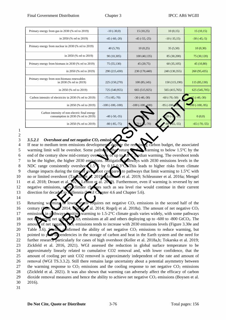
Final Government Distribution Chapter 3 IPCC AR6 WGIII
Do Not Cite, Quote or Distribute 3-76 Total pages: 156
Primary energy from gas in 2030 (% rel to 2019) -10 (-30,0) 15 (10,25) 10 (0,15) 15 (10,15)
in 2050 (% rel to 2019) -45 (-60,-20) -45 (-55,-25) -10 (-35,15) -30 (-45,-5)
Primary energy from nuclear in 2030 (% rel to 2019) 40 (5,70) 10 (0,25) 35 (5,50) 10 (0,30)
in 2050 (% rel to 2019) 90 (10,305) 100 (40,135) 85 (30,200) 75 (30,120)
Primary energy from biomass in 2030 (% rel to 2019) 75 (55,130) 45 (20,75) 60 (35,105) 45 (10,80)
in 2050 (% rel to 2019) 290 (215,430) 230 (170,440) 240 (130,355) 260 (95,435)
Primary energy from non-biomass renewables in 2030 (% rel to 2019) 225 (150,270) 100 (85,145) 150 (115,190) 115 (85,130)
in 2050 (% rel to 2019) 725 (540,955) 665 (515,925) 565 (415,765) 625 (545,705)
Carbon intensity of electricity in 2030 (% rel to 2019) -75 (-85,-70) -30 (-40,-30) -60 (-70,-50) -35 (-40,-30)
in 2050 (% rel to 2019) -100 (-100,-100) -100 (-100,-100) -95 (-100,-95) -100 (-100,-95)
Carbon intensity of non-electric final energy
consumption in 2030 (% rel to 2019) -40 (-50,-35) 0 (0,5) -20 (-30,-15) 0 (0,0)
in 2050 (% rel to 2019) -80 (-85,-75) -70 (-75,-70) -60 (-65,-55) -65 (-70,-55)
1
2
3.5.2.1 Overshoot and net negative CO2 emissions 3
If near to medium term emissions developments deplete the remaining carbon budget, the associated 4
warming limit will be overshot. Some pathways that return median warming to below 1.5°C by the 5
end of the century show mid-century overshoots of up to 1.8°C median warming. The overshoot tends 6
to be the higher, the higher 2030 emissions. Mitigation pathways with 2030 emissions levels in the 7
NDC range consistently overshoot 1.5°C by 0.15-0.3°C. This leads to higher risks from climate 8
change impacts during the time of overshoot compared to pathways that limit warming to 1.5°C with 9
no or limited overshoot (Tachiiri et al. 2019; Hofmann et al. 2019; Schleussner et al. 2016a; Mengel 10
et al. 2018; Drouet et al. 2021; Lenton et al. 2019). Furthermore, even if warming is reversed by net 11
negative emissions, other climate changes such as sea level rise would continue in their current 12
direction for decades to millennia (WGI Chapter 4.6 and Chapter 5.6). 13
14
Returning warming to lower levels requires net negative CO2 emissions in the second half of the 15
century (Fuss et al. 2014; Clarke et al. 2014; Rogelj et al. 2018a). The amount of net negative CO2 16
emissions in pathways limiting warming to 1.5-2°C climate goals varies widely, with some pathways 17
not deploying net negative CO2 emissions at all and others deploying up to -600 to -800 GtCO2. The 18
amount of net negative CO2 emissions tends to increase with 2030 emissions levels (Figure 3.30e and 19
Table 3.6). Studies confirmed the ability of net negative CO2 emissions to reduce warming, but 20
pointed to path dependencies in the storage of carbon and heat in the Earth system and the need for 21
further research particularly for cases of high overshoot (Keller et al. 2018a,b; Tokarska et al. 2019; 22
Zickfeld et al. 2016, 2021). WGI assessed the reduction in global surface temperature to be 23
approximately linearly related to cumulative CO2 removal and, with lower confidence, that the 24
amount of cooling per unit CO2 removed is approximately independent of the rate and amount of 25
removal (WGI TS.3.3.2). Still there remains large uncertainty about a potential asymmetry between 26
the warming response to CO2 emissions and the cooling response to net negative CO2 emissions 27
(Zickfeld et al. 2021). It was also shown that warming can adversely affect the efficacy of carbon 28
dioxide removal measures and hence the ability to achieve net negative CO2 emissions (Boysen et al. 29
2016). 30
31
ACCEPTED VERSION
SUBJECT TO FIN
AL EDITS
Final Government Distribution Chapter 3 IPCC AR6 WGIII
Do Not Cite, Quote or Distribute 3-77 Total pages: 156
Obtaining net negative CO2 emissions requires massive deployment of carbon dioxide removal (CDR) 1
in the second half of the century, on the order of 220 (160-370) GtCO2 for each 0.1°C degree of 2
cooling (based on the assessment of the likely range of the transient response to cumulative CO2 3
emissions in WGI Chap. 5.5, not taking into account potential asymmetries in the temperature 4
response to CO2 emissions and removals). CDR is assessed in detail in Chapter 12.3 of this report (see 5
also Cross-Chapter Box 8 in Chapter 12). Here we only point to the finding that CDR ramp-up rates 6
and absolute deployment levels are tightly limited by techno-economic, social, political, institutional 7
and sustainability constraints (Smith et al. 2016; Boysen et al. 2017; Nemet et al. 2018; Fuss et al. 8
2018, 2020; Hilaire et al. 2019; Jia et al. 2019) (Chapter 12.3). CDR therefore cannot be deployed 9
arbitrarily to compensate any degree of overshoot. A fraction of models was not able to compute 10
pathways that would follow the mitigation ambition in unconditional and conditional NDCs until 11
2030 and return warming to below 1.5°C by 2100 (Luderer et al. 2018; Roelfsema et al. 2020; Riahi 12
et al. 2021).There exists a three-way trade-off between near-term emissions developments until 2030, 13
transitional challenges during 2030-50, and long-term CDR deployment post 2050 (Sanderson et al. 14
2016; Holz et al. 2018; Strefler et al. 2018). For example, Strefler et al. (2018) find that if CO2 15
emission levels stay around 40 GtCO2 until 2030, within the range of what is projected for current 16
unconditional and conditional NDCs, rather than being halved to 20 GtCO2 until 2030, CDR 17
deployment in the second half of the century would have to increase by 50%-100%, depending on 18
whether the 2030-2050 CO2 emissions reduction rate is doubled from 6% to 12% or kept at 6% per 19
year. This three-way trade-off has also been identified at the national level (Pan et al. 2020). 20
21
In addition to enabling a temporary budget overshoot by net negative CO2 emissions in the second 22
half of the century, CDR can also be used to compensate – on an annual basis - residual CO2 23
emissions from sources that are difficult to eliminate and to reach net zero CO2 emissions more 24
rapidly if deployed before this point (Kriegler et al. 2013b; Rogelj et al. 2018a). This explains its 25
continued deployment in pathways that exclude overshoot and net negative CO2 emissions (Riahi et 26
al. 2021). However, given the timescales that would likely be needed to ramp-up CDR to Gigaton 27
scale (Nemet et al. 2018), it can be expected to only make a limited contribution to reaching net zero 28
CO2 as fast as possible. In the vast majority (95%) of 1.5-2°C mitigation pathways assessed in this 29
report, cumulative CDR deployment did not exceed 100 GtCO2 until mid-century. This adds to the 30
risk of excessively relying on CDR to compensate for weak mitigation action until 2030 by either 31
facilitating massive net CO2 emissions reduction rates during 2030-2050 or allowing a high temporary 32
overshoot of 1.5°C until the end of the century. If international burden sharing considerations are 33
taken into account, the CDR penalty for weak action could increase further, in particular for 34
developed countries (Fyson et al. 2020). Further assessment of CDR deployment in 1.5-2°C 35
mitigation pathways is found in Section 3.4.7. 36
37
3.5.2.2 Carbon lock-in and stranded assets 38
There already exists a substantial and growing carbon lock-in today, as measured by committed 39
emissions associated with existing long-lived infrastructure {Chapter 2.7, Figure 2.31}. If existing 40
fossil-fuel infrastructure would continue to be operated as historically, they would entail CO2 41
emissions exceeding the carbon budget for 1.5°C {Chapter 2.7.2, Figure 2.32}. However, owner-42
operators and societies may choose to retire existing infrastructure earlier than in the past, and 43
committed emissions are thus contingent on the competitiveness of non-emitting alternative 44
technologies and climate policy ambition. Therefore, in mitigation pathways, some infrastructure may 45
become stranded assets. Stranded assets have been defined as “assets that have suffered from 46
unanticipated or premature write-downs, devaluations or conversion to liabilities” (Caldecott 2017). 47
A systematic map of the literature on carbon lock-in has synthesized quantification of stranded-assets 48
in the mitigation pathways literature, and showed that (i) coal power plants are the most exposed to 49
ACCEPTED VERSION
SUBJECT TO FIN
AL EDITS
Final Government Distribution Chapter 3 IPCC AR6 WGIII
Do Not Cite, Quote or Distribute 3-78 Total pages: 156
risk of becoming stranded, (ii) delayed mitigation action increases stranded assets and (iii) sectoral 1
distribution and amount of stranded assets differ between countries (Fisch-Romito et al. 2020). There 2
is high agreement that existing fossil fuel infrastructure would need to be retired earlier than 3
historically, used less, or retrofitted with CCS, to stay within the remaining carbon budgets of limiting 4
warming to 1.5°C or 2°C (Johnson et al. 2016; Kefford et al. 2018; Pfeiffer et al. 2018; Cui et al. 5
2019; Fofrich et al. 2020; Rogelj et al. 2018a). Studies estimate that cumulative early retired power 6
plant capacities by 2060 can be up to 600 GW for gas and 1700 GW for coal (Iyer et al. 2015a; 7
Kefford et al. 2018), that only 42% of the total capital stock of both operating and planned coal-fired 8
powers plants can be utilized to be compatible with the 2°C target (Pfeiffer et al. 2018), and that coal-9
fired power plants in scenarios consistent with keeping global warming below 2°C or 1.5°C retire one 10
to three decades earlier than historically has been the case (Cui et al. 2019; Fofrich et al. 2020). After 11
coal, electricity production based on gas is also projected to be phased out, with some capacity 12
remaining as back-up (van Soest et al. 2017a). Kefford et al. (2018) find USD541 billion worth of 13
stranded fossil fuel power plants could be created by 2060, with China and India the most exposed. 14
Some publications have suggested that stranded long-lived assets may be even more important outside 15
of the power sector. While stranded power sector assets by 2050 could reach up to USD1.8 trillion in 16
scenarios consistent with a 2°C target, Saygin et al. (2019) found a range of USD5-11 trillion in the 17
buildings sectors. Muldoon-Smith and Greenhalgh (2019) have even estimated a potential value at 18
risk for global real estate assets up to USD21 trillion. More broadly, the set of economic activities that 19
are potentially affected by a low carbon transition is wide and includes also energy-intensive 20
industries, transport and housing, as reflected in the concept of climate policy relevant sectors 21
introduced in Battiston et al. (2017). The sectoral distribution and amount of stranded assets differ 22
across countries (Fisch-Romito et al. 2020). Capital for fossil fuel production and distribution 23
represents a larger share of potentially stranded assets in fossil fuel producing countries such as the 24
United States and Russia. Electricity generation would be a larger share of total stranded assets in 25
emerging countries because this capital is relatively new compared to its operational lifetime. 26
Conversely, buildings could represent a larger part of stranded capital in more developed countries 27
such as the United States, EU or even Russia because of high market value and low turnover rate. 28
Many quantitative estimates of stranded assets along mitigation pathways have focused on fossil fuel 29
power plants in pathways characterized by mitigation ambition until 2030 corresponding to the 30
current NDCs followed by strengthened action afterwards to limit warming to 2°C or lower (Bertram 31
et al. 2015a; Iyer et al. 2015b; Lane et al. 2016; Farfan and Breyer 2017; van Soest et al. 2017a; 32
Luderer et al. 2018; Kriegler et al. 2018a; Cui et al. 2019; Saygin et al. 2019; SEI et al. 2020). 33
Pathways following current NDCs until 2030 do not show a significant reduction of coal, oil and gas 34
use (Figure 3.30f-h, Table 3.6) compared to immediate action pathways. Stranded coal power assets 35
are evaluated to be higher by a factor of 2-3 if action is strengthened after 2030 rather than now (Iyer 36
et al. 2015b; Cui et al. 2019). There is high agreement that the later climate policies are implemented, 37
the higher the expected stranded assets and the societal, economic and political strain of strengthening 38
action. Associated price increases for carbon-intensive goods and transitional macro-economic costs 39
have been found to scale with the emissions gap in 2030 (Kriegler et al. 2013a). At the aggregate level 40
of the whole global economy, Rozenberg et al. (2015) showed that each year of delaying the start of 41
mitigation decreases the required CO2 intensity of new production by 20-50 gCO2/USD. Carbon lock-42
in can have a long-lasting effect on future emissions trajectories after 2030. Luderer et al. (2018) 43
compared cost-effective pathways with immediate action to limit warming to 1.5-2°C with pathways 44
following the NDCs until 2030 and adopting the pricing policy of the cost-effective pathways 45
thereafter and found that the majority of additional CO2 emissions from carbon lock-in occurs after 46
2030, reaching a cumulative amount of 290 (160–330) GtCO2 by 2100 (2.7.2). Early action and 47
avoidance of investments in new carbon-intensive assets can minimize these risks. 48
ACCEPTED VERSION
SUBJECT TO FIN
AL EDITS

Final Government Distribution Chapter 3 IPCC AR6 WGIII
Do Not Cite, Quote or Distribute 3-79 Total pages: 156
The risk of stranded assets has implications for workers depending from those assets, asset owners, 1
assets portfolio managers, financial institutions and the stability of the financial system. Chapter 6 2
assesses the risks and implications of stranded assets for energy systems (6.7.3, Box 6.11) and fossil 3
fuels (6.7.4). The implications of stranded assets for inequality and just transition are assessed in 4
Chapter 17 (17.3.2.3). Chapter 15 assesses the literature on those implications for the financial system 5
as well as on coping options (15.5.2, 15.6.1). 6
On the other hand, mitigation, by limiting climate change, reduces the risk of destroyed or stranded 7
assets from the physical impacts of climate change on natural and human systems, from more 8
frequent, intense or extended extreme events and from sea level rise (O’Neill et al. 2020a). The 9
literature on mitigation pathways rarely includes an evaluation of stranded assets from climate change 10
impacts. Unruh (Unruh 2019) suggest that these are the real stranded assets of carbon lock-in and 11
could prove much more costly. 12
13
3.5.2.3 Global accelerated action towards long-term climate goals 14
A growing literature explores long-term mitigation pathways with accelerated near-term action going 15
beyond the NDCs (Jiang et al. 2017; Roelfsema et al. 2018; Graichen et al. 2017; Kriegler et al. 16
2018a; van Soest et al. 2021a; Fekete et al. 2021). Global accelerated action pathways are designed to 17
transition more gradually from current policies and planned implementation of NDCs onto a 1.5-2°C 18
pathway and at the same time alleviate the abrupt transition in 2030 that would be caused by 19
following the NDCs until 2030 and strengthening towards limiting warming to 2°C thereafter (Section 20
3.5.2). Therefore they have sometimes been called bridging scenarios / pathways in the literature (IEA 21
2011; Spencer et al. 2015; van Soest et al. 2021a). They rely on regionally differentiated regulatory 22
and pricing policies to gradually strengthening regional and sectoral action beyond the mitigation 23
ambition in the NDCs. There are limitations to this approach. The tighter the warming limit, the more 24
is disruptive action becoming inevitable to achieve the speed of transition that would be required 25
(Kriegler et al. 2018a). Cost effective pathways already have abrupt shifts in deployments, 26
investments and prices at the time a stringent warming limit is imposed reflecting the fact that the 27
overall response to climate change has so far been misaligned with long-term climate goals (Geiges et 28
al. 2019; Rogelj et al. 2016; Fawcett et al. 2015; Schleussner et al. 2016b). Disruptive action can help 29
to break lock-ins and enable transformative change (Vogt-Schilb et al. 2018). 30
31
The large literature on accelerating climate action was assessed in the IPCC Special Report on 1.5°C 32
Warming (de Coninck et al. 2018) and is taken up in this report primarily in Chapters 4, 13, and 14. 33
Accelerating climate action and facilitating transformational change requires a perspective on socio-34
technical transitions (Geels et al. 2016b; Geels 2018; Geels et al. 2016a), a portfolio of policy 35
instruments to manage technological and environmental change (Goulder and Parry 2008; Fischer and 36
Newell 2008; Acemoglu et al. 2012, 2016), a notion of path dependency and policy sequencing 37
(Meckling et al. 2017; Pahle et al. 2018; Pierson 2000) and the evolvement of poly-centric governance 38
layers of institutions and norms in support of the transformation (Messner 2015; Leach et al. 2007; 39
Dietz et al. 2003). This subsection is focused on an assessment of the emerging quantitative literature 40
on global accelerated action pathways towards 1.5-2°C, which to a large extent abstracts from the 41
underlying processes and uses a number of stylized approaches to generate these pathways. A 42
representative of accelerated action pathways has been identified as one of the illustrative mitigation 43
pathways in this assessment (GS, Figure 3.31). 44
45
One approach relies on augmenting initially moderate emissions pricing policies with robust 46
anticipation of ratcheting up climate action in the future (Spencer et al. 2015). If announcements of 47
strong future climate policies are perceived to be credible, they can help to prevent carbon lock-in as 48
investors anticipating high future costs of GHG emissions would reduce investment into fossil fuel 49
infrastructure, such as coal power plants (Bauer et al. 2018b). However, the effectiveness of such 50
ACCEPTED VERSION
SUBJECT TO FIN
AL EDITS
Final Government Distribution Chapter 3 IPCC AR6 WGIII
Do Not Cite, Quote or Distribute 3-80 Total pages: 156
announcements strongly hinges on their credibility. If investors believe that policy makers could drop 1
them if anticipatory action did not occur, they may not undertake such action. 2
3
Another approach relies on international cooperation to strengthen near term climate action. These 4
studies build on international climate policy architectures that could incentivize a coalition of like-5
minded countries to raise their mitigation ambition beyond what is stated in their current NDC 6
(Graichen et al. 2017). Examples are the idea of climate clubs characterized by harmonized carbon 7
and technology markets (Pihl 2020; Nordhaus 2015; Keohane et al. 2017; Paroussos et al. 2019) and 8
the Powering Past Coal Alliance (Jewell et al. 2019). Paroussos et al. (2019) find economic benefits of 9
joining a climate club despite the associated higher mitigation effort, in particular due to access to 10
technology and climate finance. Graichen et al. (2017) find an additional reduction of 5-11 GtCO2eq 11
compared to the mitigation ambition in the NDCs from the successful implementation of international 12
climate initiatives. Other studies assess benefits from international transfers of mitigation outcomes 13
(Stua 2017; Edmonds et al. 2021). Edmonds et al. (2021) find economic gains from sharing NDC 14
emissions reduction commitments compared to purely domestic implementation of NDCs. If 15
reinvested in mitigation efforts, the study projects an additional reduction of 9 billion tonnes of CO2 in 16
2030. 17
18
The most common approach relies on strengthening regulatory policies beyond current policy trends, 19
also motivated by the finding that such policies have so far been employed more often than 20
comprehensive carbon pricing (Roelfsema et al. 2018; Kriegler et al. 2018a; van Soest et al. 2021a; 21
Fekete et al. 2021; IEA 2021a). Some studies have focused on generic regulatory policies such as low 22
carbon support policies, fossil fuel sunset policies, and resource efficiency policies (Bertram et al. 23
2015b; Hatfield-Dodds et al. 2017). Bertram et al. (2015b) found that a moderate carbon price 24
combined with a coal moratorium and ambitious low carbon support policies can limit efficiency 25
losses until 2030 if emissions pricing is raised thereafter to limit warming to 2°C. They also showed 26
that all three components are needed to achieve this outcome. Hatfield-Dodds et al. (2017) found that 27
resource efficiency can lower 2050 emissions by an additional 15-20% while boosting near-term 28
economic growth. The International Energy Agency (IEA 2021a) developed a detailed net zero 29
scenario for the global energy sector characterized by a rapid phase out of fossil fuels, a massive clean 30
energy and electrification push, and the stabilization of energy demand, leading to 10 GtCO2 lower 31
emissions from energy use in 2030 than in a scenario following the announced pledges. 32
33
The Paris Agreement has spurred the formulation of NDCs for 2030 and mid-century strategies 34
around the world (cf. Chapter 4). This is giving researchers a rich empirical basis to formulate 35
accelerated policy packages taking national decarbonisation pathways as a starting point (van Soest et 36
al. 2017b; Waisman et al. 2019; Graichen et al. 2017; Jiang et al. 2017). The concept is to identify 37
good practice policies that had demonstrable impact on pushing low carbon options or reducing 38
emissions in a country or region and then consider a wider roll-out of these policies taking into 39
account regional specificities (den Elzen et al. 2015; Kuramochi et al. 2018; Roelfsema et al. 2018; 40
Kriegler et al. 2018a; Fekete et al. 2015, 2021). A challenge for this approach is to account for the fact 41
that policy effectiveness varies with different political environments in different geographies. As a 42
result, a global roll-out of good practice policies to close the emissions gap will still be an idealized 43
benchmark, but it is useful to understand how much could be gained from it. 44
45
Accelerated action pathways derived with this approach show considerable scope for narrowing the 46
emissions gap between pathways reflecting the ambition level of the NDCs and cost-effective 47
mitigation pathways in 2030. Kriegler et al. (2018a) find around 10 GtCO2eq lower emissions 48
compared to original NDCs from a global roll-out of good practice plus net zero policies and a 49
moderate increase in regionally differentiated carbon pricing. Fekete et al. (2021) show that global 50
ACCEPTED VERSION
SUBJECT TO FIN
AL EDITS

Final Government Distribution Chapter 3 IPCC AR6 WGIII
Do Not Cite, Quote or Distribute 3-81 Total pages: 156
replication of sector progress in five major economies would reduce GHG emissions in 2030 by about 1
20% compared to a current policy scenario. These findings were found in good agreement with a 2
recent model comparison study based on results from 9 integrated assessment models (van Soest et al. 3
2021a). Based on these three studies, implementing accelerated action in terms of a global roll out of 4
regulatory and moderate pricing policies is assessed to lead to global GHG emissions of 47 (38-51) 5
GtCO2-eq in 2030 (median and 5th to 95th percentile based on 10 distinct modelled pathways). This 6
closes the implementation gap for the NDCs, and in addition falls below the emissions range implied 7
by implementing unconditional and conditional elements of NDCs by 3-9 GtCO2-eq. However, it 8
does not close the emissions gap to immediate action pathways likely limiting warming to 2°C, and, 9
based on our assessment in Section 3.5.2, emission levels above 40 GtCO2-eq in 2030 still have a very 10
low prospect for keeping limiting warming to 1.5°C with no or limited overshoot in reach. 11
12
Figure 3.31 shows the intermediate position of accelerated action pathways derived by van Soest et al. 13
(2021a) between pathways that follow the NDCs until 2030 and immediate action pathways likely 14
limiting warming to 2°C. Accelerated action is able to reduce the abrupt shifts in emissions, fossil fuel 15
use and low carbon power generation in 2030 and also limits peak warming more effectively than 16
NDC pathways. But primarily due to the moderate carbon price assumptions (Fig. 3.31b), the 17
reductions in emissions and particular fossil fuel use are markedly smaller than what would be 18
obtained in the case of immediate action. The assessment shows that accelerated action until 2030 can 19
have significant benefits in terms of reducing the mitigation challenges from following the NDCs 20
until 2030. But putting a significant value on GHG emissions reductions globally remains a key 21
element of moving onto 1.5-2°C pathways. The vast majority of pathways that limit warming to 2°C 22
or below, independently of their differences in near term emission developments, converge to a global 23
mitigation regime putting such a significant value on GHG emission reductions in all regions and 24
sectors. 25
ACCEPTED VERSION
SUBJECT TO FIN
AL EDITS

Final Government Distribution Chapter 3 IPCC AR6 WGIII
Do Not Cite, Quote or Distribute 3-82 Total pages: 156
1 2
Figure 3.31: Comparison of (i) pathways with immediate action likely limiting warming to 2°C 3 (Immediate, light blue), (ii) pathways following the NDCs until 2030 and aiming to likely stay below 2°C 4
thereafter (NDC; orange) and (iii) pathways accelerating near term action until 2030 beyond NDC 5 ambition levels and aiming to likely stay below 2°C thereafter (Accelerated) for selected indicators as 6
listed in the panel titles, based on pathways from van Soest et al. (2021a). Low carbon electricity 7 comprises renewable and nuclear power. Indicator ranges are shown as boxplots (full range, interquartile 8
range, and median) for the years 2030, 2050 and 2100 (absolute values) and for the periods 2020-2030, 9 2030-2050 (change indicators). Ranges are based on nine models participating in (van Soest et al. 2021a) 10 with only 7 models reporting emissions and climate results and 8 models reporting carbon prices. The 11 purple dot denotes the illustrative mitigation pathway GS that was part of the study by van Soest et al. 12
13
14
3.6 Economics of long-term mitigation and development pathways, 15
including mitigation costs and benefits 16
A complete appraisal of economic effects and welfare effects at different temperature levels would 17
include the macroeconomic impacts of investments in low-carbon solutions and structural change 18
away from emitting activities, co-benefits and adverse side effects of mitigation, (avoided) climate 19
ACCEPTED VERSION
SUBJECT TO FIN
AL EDITS

Final Government Distribution Chapter 3 IPCC AR6 WGIII
Do Not Cite, Quote or Distribute 3-83 Total pages: 156
damages, as well as (reduced) adaptation costs, with high temporal, spatial and social heterogeneity 1
using a harmonized framework. If no such complete appraisal in a harmonized framework exists, key 2
elements are emerging from the literature, and assessed in the following subsections: on aggregated 3
economy-wide global mitigation costs (section 3.6.1), on the economic benefits of avoiding climate 4
impacts (section 3.6.2), on economic benefits and costs associated with mitigation co-benefits and co-5
harms (section 3.6.3) and on the distribution of economic implications between economic sectors and 6
actors (section 3.6.4). 7
8
3.6.1 Economy-wide implications of mitigation 9
3.6.1.1 Global economic effects of mitigation and carbon values in mitigation pathways 10
11
START BOX HERE 12
13
Box 3.5 Concepts and modelling frameworks used for quantifying macro-economic effects of mitigation 14
Most studies that have developed mitigation pathways have used a Cost-effectiveness analysis (CEA) 15
framework, which aim at comparing the costs of different mitigation strategies designed to meet a 16
given climate change mitigation goal (e.g., an emission-reduction target or a temperature stabilization 17
target) but does not represent economic impacts from climate change itself, nor the associated 18
economic benefits of avoided impacts. Other studies use modelling frameworks that represent the 19
feedback of damages from climate change on the economy in a Cost-benefit analysis (CBA) 20
approach, which balances mitigation costs and benefits. This second type of studies is represented in 21
section 3.6.2. 22
The marginal abatement cost of carbon, also called carbon price, is determined by the mitigation 23
target under consideration: it describes the cost of reducing the last unit of emissions to reach the 24
target at a given point in time. Total macro-economic mitigation costs (or gains) aggregate the 25
economy-wide impacts of investments in low-carbon solutions and structural changes away from 26
emitting activities. The total macro-economic effects of mitigation pathways are reported in terms of 27
variations in economic output or consumption levels, measured against a Reference Scenario, also 28
called Baseline, at various points in time or discounted over a given time period. Depending on the 29
study, the Reference Scenario reflects specific assumptions about patterns of socio-economic 30
development and assumes either no climate policies or the climate policies in place or planned at the 31
time the study was carried out. When available in the AR6 scenarios database, this second type of 32
Reference Scenario, with current policies, has been chosen for computation of mitigation costs. In the 33
vast majority of studies that have produced the body of work on the cost of mitigation assessed here, 34
and in particular in all studies that have submitted global scenarios to the AR6 scenarios database 35
except (Schultes et al. 2021), the feedbacks of climate change impacts on the economic development 36
pathways are not accounted for. This omission of climate impacts leads to overly optimistic economic 37
projections in the reference scenarios, in particular in reference scenarios with no or limited mitigation 38
action where the extent of global warming is the greatest. Mitigation cost estimates computed against 39
no or limited policy reference scenarios therefore omit economic benefits brought by avoided climate 40
change impact along mitigation pathways, and should be interpreted with care (Grant et al. 2020). 41
When aggregate economic benefits from avoided climate change impacts are accounted for, 42
mitigation is a welfare-enhancing strategy (see section 3.6.2). 43
If GDP or consumption in mitigation pathways are below the reference scenario levels, they are 44
reported as losses or macro-economic costs. Such cost estimates give an indication on how economic 45
activity slows relative to the reference scenario; they do not necessarily describe, in absolute terms, a 46
reduction of economic output or consumption levels relative to previous years along the pathway. 47
Aggregate mitigation costs depend strongly on the modelling framework used and the assumptions 48
ACCEPTED VERSION
SUBJECT TO FIN
AL EDITS
Final Government Distribution Chapter 3 IPCC AR6 WGIII
Do Not Cite, Quote or Distribute 3-84 Total pages: 156
about the reference scenario against which mitigation costs are measured, in particular whether the 1
reference scenario is, or not, on the efficiency frontier of the economy. If the economy is assumed to 2
be at the efficiency frontier in the reference scenario, mitigation inevitably leads to actual costs, at 3
least in the short run until the production frontier evolves with technical and structural change. 4
Starting from a reference scenario that is not on the efficiency frontier opens the possibility to 5
simultaneously reduce emissions and obtain macroeconomic gains, depending on the design and 6
implementation of mitigation policies. A number of factors can result in reference scenarios below the 7
efficiency frontier, for instance distorting labour taxes and/or fossil fuel subsidies, misallocation or 8
under-utilization of production factors such as involuntary unemployment, imperfect information or 9
non-rational behaviours. Although these factors are pervasive, the modelling frameworks used to 10
construct mitigation pathways are often limited in their ability to represent them (Köberle et al. 2021). 11
The absolute level of economic activity and welfare also strongly depends on the socioeconomic 12
pathway assumptions regarding inter alia evolutions in demography, productivity, education levels, 13
inequality and technical change and innovation. The GDP or consumption indicators reported in the 14
database of scenarios, and synthesized below, represent the absolute level of aggregate economic 15
activity or consumption but do not reflect welfare and well-being (Roberts et al. 2020), that notably 16
depend on human needs satisfaction, distribution within society and inequality (see section 3.6.4). 17
Chapter 1 and Annex III give further elements on the economic concepts and on the modelling 18
frameworks, including their limitations, used in this report, respectively. 19
END BOX HERE 20
21
Estimates for the marginal abatement cost of carbon in mitigation pathways vary widely, depending 22
on the modelling framework used and socioeconomic, technological and policy assumptions. 23
However, it is robust across modelling frameworks that the marginal abatement cost of carbon 24
increases for lower temperature categories, with a higher increase in the short-term than in the longer-25
term (Figure 3.32, left panel) (high confidence). The marginal abatement cost of carbon increases non-26
linearly with the decrease of CO2 emissions level, but the uncertainty in the range of estimates also 27
increases (Figure 3.33). Mitigation pathways with low‐energy consumption patterns exhibit lower 28
carbon values (Méjean et al. 2019; Meyer et al. 2021). In the context of the COVID-19 pandemic 29
recovery, Kikstra et al. (2021a) also show that a low energy demand recovery scenario reduces carbon 30
prices for a 1.5°C consistent pathway by 19% compared to a scenario with energy demand trends 31
restored to pre-pandemic levels. 32
33
For optimization modelling frameworks, the time profile of marginal abatement costs of carbon 34
depends on the discount rate, with lower discount rates implying higher carbon values in the short 35
term but lower values in the long term (Emmerling et al. 2019) (see also Discounting in glossary and 36
Annex III part I section 2). In that case, the discount rate also influences the shape of the emissions 37
trajectory, with low discount rates implying more emission reduction in the short-term and, for low 38
temperature categories, limiting CDR and temperature overshoot. 39
40
Pathways that correspond to NDCs in 2030 and strengthen action after 2030 imply higher marginal 41
abatement costs of carbon in the longer run than pathways with stronger immediate global mitigation 42
action (Figure 3.32, right panel) (high confidence). 43
44
ACCEPTED VERSION
SUBJECT TO FIN
AL EDITS
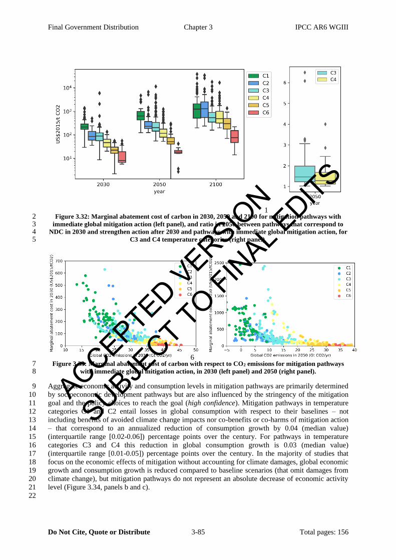
Final Government Distribution Chapter 3 IPCC AR6 WGIII
Do Not Cite, Quote or Distribute 3-85 Total pages: 156
1 Figure 3.32: Marginal abatement cost of carbon in 2030, 2050 and 2100 for mitigation pathways with 2
immediate global mitigation action (left panel), and ratio in 2050 between pathways that correspond to 3 NDC in 2030 and strengthen action after 2030 and pathways with immediate global mitigation action, for 4
C3 and C4 temperature categories (right panel). 5
6 Figure 3.33: Marginal abatement cost of carbon with respect to CO2 emissions for mitigation pathways 7
with immediate global mitigation action, in 2030 (left panel) and 2050 (right panel). 8
Aggregate economic activity and consumption levels in mitigation pathways are primarily determined 9
by socioeconomic development pathways but are also influenced by the stringency of the mitigation 10
goal and the policy choices to reach the goal (high confidence). Mitigation pathways in temperature 11
categories C1 and C2 entail losses in global consumption with respect to their baselines – not 12
including benefits of avoided climate change impacts nor co-benefits or co-harms of mitigation action 13
– that correspond to an annualized reduction of consumption growth by 0.04 (median value) 14
(interquartile range [0.02-0.06]) percentage points over the century. For pathways in temperature 15
categories C3 and C4 this reduction in global consumption growth is 0.03 (median value) 16
(interquartile range [0.01-0.05]) percentage points over the century. In the majority of studies that 17
focus on the economic effects of mitigation without accounting for climate damages, global economic 18
growth and consumption growth is reduced compared to baseline scenarios (that omit damages from 19
climate change), but mitigation pathways do not represent an absolute decrease of economic activity 20
level (Figure 3.34, panels b and c). 21
22
ACCEPTED VERSION
SUBJECT TO FIN
AL EDITS
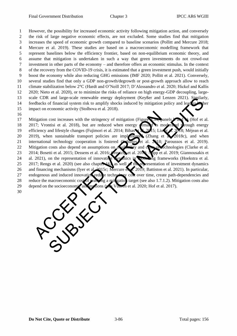
Final Government Distribution Chapter 3 IPCC AR6 WGIII
Do Not Cite, Quote or Distribute 3-86 Total pages: 156
However, the possibility for increased economic activity following mitigation action, and conversely 1
the risk of large negative economic effects, are not excluded. Some studies find that mitigation 2
increases the speed of economic growth compared to baseline scenarios (Pollitt and Mercure 2018; 3
Mercure et al. 2019). These studies are based on a macroeconomic modelling framework that 4
represent baselines below the efficiency frontier, based on non-equilibrium economic theory, and 5
assume that mitigation is undertaken in such a way that green investments do not crowd-out 6
investment in other parts of the economy – and therefore offers an economic stimulus. In the context 7
of the recovery from the COVID-19 crisis, it is estimated that a green investment push, would initially 8
boost the economy while also reducing GHG emissions (IMF 2020; Pollitt et al. 2021). Conversely, 9
several studies find that only a GDP non-growth/degrowth or post-growth approach allow to reach 10
climate stabilization below 2°C (Hardt and O’Neill 2017; D’Alessandro et al. 2020; Hickel and Kallis 11
2020; Nieto et al. 2020), or to minimize the risks of reliance on high energy-GDP decoupling, large-12
scale CDR and large-scale renewable energy deployment (Keyßer and Lenzen 2021). Similarly, 13
feedbacks of financial system risk to amplify shocks induced by mitigation policy and lead to higher 14
impact on economic activity (Stolbova et al. 2018). 15
16
Mitigation cost increases with the stringency of mitigation (Figure 3.34, panels b and c) (Hof et al. 17
2017; Vrontisi et al. 2018), but are reduced when energy demand is moderated through energy 18
efficiency and lifestyle changes (Fujimori et al. 2014; Bibas et al. 2015; Liu et al. 2018; Méjean et al. 19
2019), when sustainable transport policies are implemented (Zhang et al. 2018c), and when 20
international technology cooperation is fostered (Schultes et al. 2018; Paroussos et al. 2019). 21
Mitigation costs also depend on assumptions on availability and costs of technologies (Clarke et al. 22
2014; Bosetti et al. 2015; Dessens et al. 2016; Creutzig et al. 2018; Napp et al. 2019; Giannousakis et 23
al. 2021), on the representation of innovation dynamics in modelling frameworks (Hoekstra et al. 24
2017; Rengs et al. 2020) (see also chapter 16), as well as the representation of investment dynamics 25
and financing mechanisms (Iyer et al. 2015c; Mercure et al. 2019; Battiston et al. 2021). In particular, 26
endogenous and induced innovation reduce technology cost over time, create path-dependencies and 27
reduce the macroeconomic cost of reaching a mitigation target (see also 1.7.1.2). Mitigation costs also 28
depend on the socioeconomic assumptions (van Vuuren et al. 2020; Hof et al. 2017). 29
30
ACCEPTED VERSION
SUBJECT TO FIN
AL EDITS
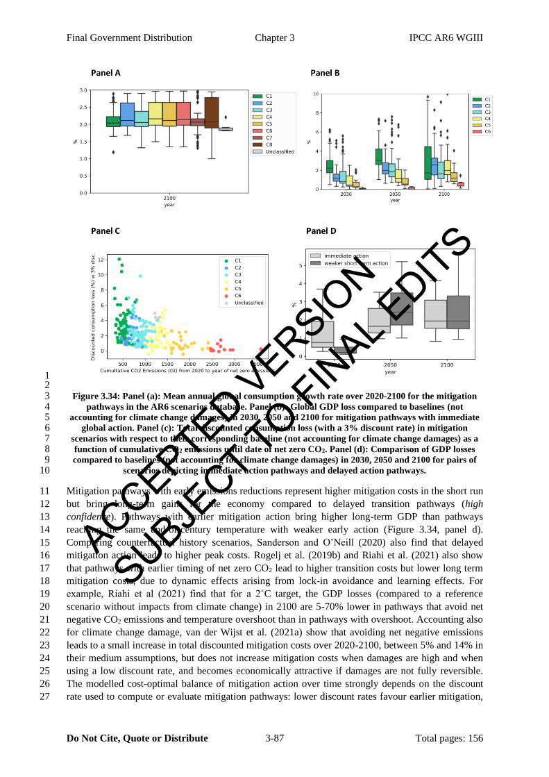
Final Government Distribution Chapter 3 IPCC AR6 WGIII
Do Not Cite, Quote or Distribute 3-87 Total pages: 156
1 2
Figure 3.34: Panel (a): Mean annual global consumption growth rate over 2020-2100 for the mitigation 3 pathways in the AR6 scenarios database. Panel (b): Global GDP loss compared to baselines (not 4
accounting for climate change damages) in 2030, 2050 and 2100 for mitigation pathways with immediate 5 global action. Panel (c): Total discounted consumption loss (with a 3% discount rate) in mitigation 6
scenarios with respect to their corresponding baseline (not accounting for climate change damages) as a 7 function of cumulative CO2 emissions until date of net zero CO2. Panel (d): Comparison of GDP losses 8 compared to baselines (not accounting for climate change damages) in 2030, 2050 and 2100 for pairs of 9
scenarios depicting immediate action pathways and delayed action pathways. 10
Mitigation pathways with early emissions reductions represent higher mitigation costs in the short run 11
but bring long-term gains for the economy compared to delayed transition pathways (high 12
confidence). Pathways with earlier mitigation action bring higher long-term GDP than pathways 13
reaching the same end-of-century temperature with weaker early action (Figure 3.34, panel d). 14
Comparing counterfactual history scenarios, Sanderson and O’Neill (2020) also find that delayed 15
mitigation action leads to higher peak costs. Rogelj et al. (2019b) and Riahi et al. (2021) also show 16
that pathways with earlier timing of net zero CO2 lead to higher transition costs but lower long term 17
mitigation costs, due to dynamic effects arising from lock-in avoidance and learning effects. For 18
example, Riahi et al (2021) find that for a 2˚C target, the GDP losses (compared to a reference 19
scenario without impacts from climate change) in 2100 are 5-70% lower in pathways that avoid net 20
negative CO2 emissions and temperature overshoot than in pathways with overshoot. Accounting also 21
for climate change damage, van der Wijst et al. (2021a) show that avoiding net negative emissions 22
leads to a small increase in total discounted mitigation costs over 2020-2100, between 5% and 14% in 23
their medium assumptions, but does not increase mitigation costs when damages are high and when 24
using a low discount rate, and becomes economically attractive if damages are not fully reversible. 25
The modelled cost-optimal balance of mitigation action over time strongly depends on the discount 26
rate used to compute or evaluate mitigation pathways: lower discount rates favour earlier mitigation, 27
ACCEPTED VERSION
SUBJECT TO FIN
AL EDITS
Final Government Distribution Chapter 3 IPCC AR6 WGIII
Do Not Cite, Quote or Distribute 3-88 Total pages: 156
reducing both temperature overshoot and reliance on net negative carbon emissions (Emmerling et al. 1
2019; Riahi et al. 2021). Mitigation pathways with weak early action corresponding to NDCs in 2030 2
and strengthening action after 2030 to reach end-of-century temperature targets imply limited 3
mitigation costs in 2030, compared to immediate global action pathways, but faster increase in costs 4
post-2030, with implications for intergenerational equity (Aldy et al. 2016; Liu et al. 2016; Vrontisi et 5
al. 2018). Emissions trading policies reduce global aggregate mitigation costs, in particular in the 6
context of achieving NDCs (Fujimori et al. 2015, 2016a; Edmonds et al. 2021; Böhringer et al. 2021), 7
and change the distribution of mitigation costs between regions and countries (see section 3.6.1.2). 8
9
3.6.1.2 Regional mitigation costs and effort-sharing regimes 10
The economic repercussions of mitigation policies vary across countries (Hof et al. 2017; Aldy et al. 11
2016): regional variations exist in institutions, economic and technological development, and 12
mitigation opportunities. For a globally uniform carbon price, carbon intensive and energy exporting 13
countries bear the highest economic costs because of a deeper transformation of their economies and 14
of trade losses in the fossil markets (Stern et al. 2012; Tavoni et al. 2015; Böhringer et al. 2021). This 15
finding is confirmed in 16
Figure 3.35. Since carbon intensive countries are often poorer, uniform global carbon prices raises 17
equity concerns (Tavoni et al. 2015). On the other hand, the climate economic benefits of mitigating 18
climate change will be larger in poorer countries (Cross-Working Group Box 1). This reduces policy 19
regressivity but does not eliminate it (Taconet et al. 2020; Gazzotti et al. 2021). Together with co-20
benefits, such as health benefits of improved air quality, the economic benefits of mitigating climate 21
change are likely to outweigh mitigation costs in many regions (Li et al. 2018, 2019; Scovronick et al. 22
2021). 23
24
Regional policy costs depend on the evaluation framework (Budolfson et al. 2021), policy design, 25
including revenue recycling, and on international coordination, especially among trade partners. By 26
fostering technological change and finance, climate cooperation can generate economic benefits, both 27
in large developing economies such as China and India (Paroussos et al. 2019) and industrialized 28
countries such as Europe (Vrontisi et al. 2020). International coordination is a major driver of regional 29
policy costs. Delayed participation in global mitigation efforts raises participation costs, especially in 30
carbon intensive economies ( 31
Figure 3.35, right panel). Trading systems and transfers can deliver cost savings and improve equity 32
(Rose et al. 2017a). On the other hand, measures that reduce imports of energy intensive goods such 33
as carbon border tax adjustment may imply costs outside of the policy jurisdiction and have 34
international equity repercussions, depending on how they are designed (Böhringer et al. 2012, 2017; 35
Cosbey et al. 2019) (see also 13.6.6). 36
37
An equitable global emission trading scheme would require very large international financial 38
transfers, in the order of several hundred billion USD per year (Tavoni et al. 2015; van den Berg et al. 39
2020; Bauer et al. 2020). The magnitude of transfers depends on the stringency of the climate goals 40
and on the burden sharing principle. Equitable burden sharing compliant with the Paris Agreement 41
leads to negative carbon allowances for developed countries as well as China by mid-century (van den 42
Berg et al. 2020), more stringent than cost-optimal pathways. International transfers also depend on 43
the underlying socio-economic development (Leimbach and Giannousakis 2019), as these drive the 44
mitigation costs of meeting the Paris Agreement (Rogelj et al. 2018b). By contrast, achieving equity 45
without international markets would result in a large discrepancy in regional carbon prices, up to a 46
factor (Bauer et al. 2020). The efficiency-sovereignty trade-off can be partly resolved by allowing for 47
limited differentiation of regional carbon prices: moderate financial transfers substantially reduce 48
inefficiencies by narrowing the carbon price spread (Bauer et al. 2020). 49
ACCEPTED VERSION
SUBJECT TO FIN
AL EDITS

Final Government Distribution Chapter 3 IPCC AR6 WGIII
Do Not Cite, Quote or Distribute 3-89 Total pages: 156
1 2
Figure 3.35: Left panel: Regional mitigation costs in the year 2050 (expressed as GDP losses between 3 mitigation scenarios and corresponding baselines, not accounting for climate change damages), under the 4 assumption of immediate global action with uniform global carbon pricing and no international transfers, 5 by climate categories for the 2°C and 1.5°C (with and without overshoot) categories. Right panel: Policy 6
costs in 2050 (as in panel a) for 1.5-2°C climate categories for scenario pairs that represent either 7 immediate global action (‘immediate’) or delayed global action (‘delayed’) with weaker action in the 8
short-term, strengthening to reach the same end-of-century temperature target. 9
10
3.6.1.3 Investments in mitigation pathways 11
Figure 3.36 and Figure 3.37 show increased investment needs in the energy sector in lower 12
temperature categories, and a major shift away from fossil generation and extraction towards 13
electricity, including for system enhancements for electricity transmission, distribution and storage, 14
and low-carbon technologies. Investment needs in the electricity sector are USD2.3 trillion 2015 yr-1 15
over 2023-2050 on average for C1 pathways, USD2.0 trillion for C2 pathways, USD1.7 trillion for 16
C3, USD1.2 trillion for C4 and USD0.9-1.1 billion for C5/C6/C7 (mean values for pathways in each 17
temperature categories). The regional pattern of power sector investments broadly mirrors the global 18
picture. However, the bulk of investment requirements are in medium- and low-income regions. 19
These results from the AR6 scenarios database corroborate the findings from McCollum et al. 20
(2018a), Zhou et al. (2019) and Bertram et al. (2021). 21
22
In the context of the COVID-19 pandemic recovery, (Kikstra et al. 2021a) show that a low energy 23
demand recovery scenario reduces energy investments required until 2030 for a 1.5°C consistent 24
pathway by 9% (corresponding to reducing total required energy investment by USD1.8 trillion) 25
compared to a scenario with energy demand trends restored to pre-pandemic levels. 26
27 ACCEPTED VERSION
SUBJECT TO FIN
AL EDITS

Final Government Distribution Chapter 3 IPCC AR6 WGIII
Do Not Cite, Quote or Distribute 3-90 Total pages: 156
1 Figure 3.36: Global average yearly investments from 2023-2052 for 9 electricity supply subcomponents 2
and for extraction of fossil fuels (in billion USD2015), in pathways by temperature categories. T&D: 3 transmission and distribution of electricity. Bars show the median values (number of pathways at the 4
bottom), and whiskers the interquartile ranges. 5
6 Figure 3.37: Average yearly investments from 2023-2052 for the four subcomponents of the energy 7 system representing the larger amounts (in billion USD2015), by aggregate regions, in pathways by 8
temperature categories. T&D: transmissions and distribution of electricity. Extr.: extraction of fossil 9
ACCEPTED VERSION
SUBJECT TO FIN
AL EDITS
Final Government Distribution Chapter 3 IPCC AR6 WGIII
Do Not Cite, Quote or Distribute 3-91 Total pages: 156
fuels. Bars show the median values (number of pathways at the bottom), and whiskers the interquartile 1 ranges. 2
3
Few studies extend the scope of the investment needs quantification beyond the energy sector. Fisch-4
Romito and Guivarch (2019) and Ó Broin and Guivarch (2017) assess investment needs for 5
transportation infrastructures and find lower investment needs in low-carbon pathways, due to a 6
reduction in transport activity and a shift towards less road construction, compared to high-carbon 7
pathways. Rozenberg and Fay (2019) estimate the funding needs to close the service gaps in water 8
and sanitation, transportation, electricity, irrigation, and flood protection in thousands of scenarios, 9
showing that infrastructure investment paths compatible with full decarbonization in the second half 10
of the century need not cost more than more-polluting alternatives. Investment needs are estimated 11
between 2 percent and 8 percent of GDP, depending on the quality and quantity of services targeted, 12
the timing of investments, construction costs, and complementary policies. 13
14
Chapter 15 also reports investment requirements in global mitigation pathways in the near-term, 15
compares them to recent investment trends, and assesses financing issues. 16
17
3.6.2 Economic benefits of avoiding climate changes impacts 18
19
START BOX HERE 20
21
Cross-Working Group Box 1: Economic benefits from avoided climate impacts along long-term 22
mitigation pathways 23
Authors: Céline Guivarch (France), Steven Rose (the United States of America), Alaa Al Khourdajie 24
(United Kingdom/Syria), Valentina Bosetti (Italy), Edward Byers (Austria/Ireland), Katherine Calvin 25
(the United States of America), Tamma Carleton (the United States of America), Delavane Diaz (the 26
United States of America), Laurent Drouet (France/Italy), Michael Grubb (United Kingdom), Tomoko 27
Hasegawa (Japan), Alexandre C. Köberle (Brazil/ United Kingdom), Elmar Kriegler (Germany), 28
David McCollum (the United States of America), Aurélie Méjean (France), Brian O’Neill (the United 29
States of America), Franziska Piontek (Germany), Julia Steinberger (United Kingdom/Switzerland), 30
Massimo Tavoni (Italy) 31
32
Mitigation reduces the extent of climate change and its impacts on ecosystems, infrastructure, and 33
livelihoods. This box summarizes elements from the WGII report on aggregate climate change 34
impacts and risks, putting them into the context of mitigation pathways. AR6 Working Group II 35
provides an assessment of current lines of evidence regarding potential climate risks with future 36
climate change, and therefore, the avoided risks from mitigating climate change. Regional and 37
sectoral climate risks to physical and social systems are assessed (WGII Chapters 2-15). Over 100 of 38
these are identified as Key Risks (KRs) and further synthesized by WGII Chapter 16 into eight 39
overarching Representative Key Risks (RKRs) relating to low-lying coastal systems; terrestrial and 40
ocean ecosystems; critical physical infrastructure, networks and services; living standards; human 41
health; food security; water security; and peace and mobility (WGII 16.5.2). The RKR assessment 42
finds that risks increase with global warming level, and also depend on socioeconomic development 43
conditions, which shape exposure and vulnerability, and adaptation opportunities and responses. 44
“Reasons For Concern”, another WGII aggregate climate impacts risk framing, are also assessed to 45
increase with climate change, with increasing risk for unique and threatened systems, extreme weather 46
events, distribution of impacts, global aggregate impacts, and large-scale singular events (WGII 47
Chapter 16). For human systems, in general, the poor and disadvantaged are found to have greater 48
exposure level and vulnerability for a given hazard. With some increase in global average warming 49
ACCEPTED VERSION
SUBJECT TO FIN
AL EDITS

Final Government Distribution Chapter 3 IPCC AR6 WGIII
Do Not Cite, Quote or Distribute 3-92 Total pages: 156
from today expected regardless of mitigation efforts, human and natural systems will be exposed to 1
new conditions and additional adaptation will be needed (WGII Chapter 18). The range of dates for 2
when a specific warming level could be reached depends on future global emissions, with significant 3
overlap of ranges across emissions scenarios due to climate system response uncertainties (WGI 4
Tables 4.2 and 4.5). The speed at which the climate changes is relevant to adaptation timing, 5
possibilities, and net impacts. 6
7
WGII also assesses the growing literature estimating the global aggregate economic impacts of 8
climate change and the social cost of carbon dioxide and other greenhouse gases (Cross-Working Box 9
Economic: Estimating Global Economic Impacts from Climate Change and the Social Cost of 10
Carbon”, in WGII Chapter 16). The former represents aggregate estimates that inform assessment of 11
the economic benefits of mitigation. This literature is characterized by significant variation in the 12
estimates, including for today's level of global warming, due primarily to fundamental differences in 13
methods, but also differences in impacts included, representation of socioeconomic exposure, 14
consideration of adaptation, aggregation approach, and assumed persistence of damages. WGII’s 15
assessment identifies different approaches to quantification of aggregated economic impacts of 16
climate change, including: physical modelling of impact processes, such as projected mortality rates 17
from climate risks such as heat, vector- or waterborne diseases that are then monetized; structural 18
economic modelling of impacts on production, consumption, and markets for economic sectors and 19
regional economies; and statistical estimation of impacts based on observed historical responses to 20
weather and climate. WGII finds that variation in estimated global economic impacts increases with 21
warming in all methodologies, indicating higher risk in terms of economic impacts at higher 22
temperatures (high confidence). Many estimates are nonlinear with marginal economic impacts 23
increasing with temperature, although some show declining marginal economic impacts with 24
temperature, and functional forms cannot be determined for all studies. WGII’s assessment finds that 25
the lack of comparability between methodologies does not allow for identification of robust ranges of 26
global economic impact estimates (high confidence). Further, WGII identifies evaluating and 27
reconciling differences in methodologies as a research priority for facilitating use of the different lines 28
of evidence (high confidence). However, there are estimates that are higher than AR5, indicating that 29
global aggregate economic impacts could be higher than previously estimated (low confidence due to 30
the lack of comparability across methodologies and lack of robustness of estimates) (Cross-Working 31
Box Economic). 32
33
Conceptually, the difference in aggregate economic impacts from climate change between two given 34
temperature levels represents the aggregate economic benefits arising from avoided climate change 35
impacts due to mitigation action. A subset of the studies whose estimates were evaluated by WGII (5 36
of 15) are used to derive illustrative estimates of aggregate economic benefits in 2100 arising from 37
avoided climate change (Howard and Sterner 2017; Burke et al. 2018; Pretis et al. 2018; Kahn et al. 38
2019; Takakura et al. 2019). Burke et al. (2018), Pretis et al. (2018) and Kahn et al. (2019) are 39
examples of statistical estimation of historical relationships between temperature and economic 40
growth, whereas Takakura et al. (2019) is an example of structural modelling, which evaluates 41
selected impact channels (impacts on agriculture productivity, undernourishment, heat-related 42
mortality, labour productivity, cooling/heating demand, hydroelectric and thermal power generation 43
capacity and fluvial flooding) with a general equilibrium model. Howard and Sterner (2017) and 44
Rose et al. (2017b) estimate damage functions that can be used to compute the economic benefits of 45
mitigation from avoiding a given temperature level for a lower one. Howard and Sterner (2017) 46
estimate a damage function from a meta-analysis of aggregate economic impact studies, while Rose et 47
al. (2017b) derive global functions by temperature and socioeconomic drivers from stylized aggregate 48
Cost-Benefit-Analysis integrated assessment models using diagnostic experiments. Cross-Working 49
Group Box 1 Figure 1 summarizes the global aggregate economic benefits in 2100 of avoided climate 50
ACCEPTED VERSION
SUBJECT TO FIN
AL EDITS
Final Government Distribution Chapter 3 IPCC AR6 WGIII
Do Not Cite, Quote or Distribute 3-93 Total pages: 156
change impacts from individual studies corresponding to shifting from a higher temperature category 1
(above 3°C, below 3°C or below 2.5°C) to below 2°C, as well as from below 2°C to below 1.5°C. 2
Benefits are positive and increase with the temperature gap for any given study, and this result is 3
robust across socioeconomic scenarios. The Figure provides evidence of a wide range of 4
quantifications, and illustrates the important differences associated with methods. Panel a puts the 5
studies used to calculate aggregate economic benefits arising from avoided impacts into the context of 6
the broader set of studies assessed in WGII (WGII Cross-Working Group Box Economic, 16.6.2). 7
However, economic benefits in 2100 arising from avoided impacts cannot be directly computed from 8
damage estimates across this broader set of studies, due to inconsistencies - different socioeconomic 9
assumptions, scenario designs, and counterfactual reference scenarios across studies. Furthermore, 10
these types of estimates cannot be readily compared to mitigation cost estimates. The comparison 11
would require a framework that ensures consistency in assumptions and dynamics and allows for 12
consideration of benefits and costs along the entire pathway. 13
14
Cross-Working Group Box 1 Figure 1: Global aggregate economic benefits of mitigation from avoided 15 climate change impacts in 2100 corresponding to shifting from a higher temperature category (4°C 16
(3.75°C-4.25°C), 3°C(2.75°C-3.25°C) or above 2°C (2°C-2.5°C)) to below 2°C (1.5°C-2°C), as well as from 17 below 2°C to below 1.5°C (1°C-1.5°C), from the five studies discussed in the text. Panel a is adapted from 18
WGII CWGB ECONOMIC Figure 1, showing global aggregate economic impact estimates (% global 19 GDP loss relative to GDP without additional climate change) by temperature change level. All estimates 20
are shown in grey. Estimates used for the computation of estimated benefits in 2100 in Panel b are 21 coloured for the selected studies, which provide results for different temperature change levels. See the 22 WGII Chapter 16 box for discussion and assessment of the estimates in Panel a and the differences in 23
methodologies. For B18 and T19, median estimates in the cluster are considered. Shape distinguishes the 24 baseline scenarios. Temperature ranges are highlighted. HS17 estimates are based on their preferred 25 model - 50th percentile of non-catastrophic damage. Panel b shows the implied aggregate economic 26
benefits in 2100 of a lower temperature increase. Economic benefits for point estimates are computed as a 27 difference, while economic benefits from the curve HS17 are computed as ranges from the segment 28
differences. 29 30
Aggregate benefits from avoided impacts expressed in GDP terms, as in Figure 1, do not encompass 31
all avoided climate risks, adaptation possibilities, and does not represent their influence on well-being 32
and welfare (WGII Cross-Working Group Box Economic). Methodological challenges for economic 33
impact estimates include representing uncertainty and variability, capturing interactions and spill 34
overs, considering distributional effects, representing micro and macro adaptation processes, 35
specifying non-gradual damages and non-linearities, and improving understanding of potential long-36
run growth effects. In addition, the economic benefits aggregated at the global scale provide limited 37
insights into regional heterogeneity. Global economic impact studies with regional estimates find 38
large differences across regions in absolute and percentage terms, with developing and transitional 39
economies typically more vulnerable. Furthermore, (avoided) impacts for poorer households and 40
poorer countries can represent a smaller share in aggregate quantifications expressed in GDP terms or 41
monetary terms, compared to their influence on well-being and welfare (Hallegatte et al. 2020; 42
Markhvida et al. 2020). Finally, as noted by WGII, other lines of evidence regarding climate risks, 43
beyond monetary estimates, should be considered in decision-making, including key risks and 44
Reasons for Concern. 45
46
END CCB HERE 47
48
Cost-benefit analyses (CBA) aim to balance all costs and benefits in a unified framework (Nordhaus, 49
2008). Estimates of economic benefits from avoided climate change impacts depend on the types of 50
damages accounted for, the assumed exposure and vulnerability to these damages as well as the 51
adaptation capacity, which in turn are based on the development pathway assumed (Cross-Working 52
ACCEPTED VERSION
SUBJECT TO FIN
AL EDITS
Final Government Distribution Chapter 3 IPCC AR6 WGIII
Do Not Cite, Quote or Distribute 3-94 Total pages: 156
Group Box 1). CBA integrated assessment models raised critics, in particular for omitting elements of 1
dynamic realism, such as inertia, induced innovation and path dependence, in their representation of 2
mitigation (Grubb et al. 2021), and for underestimating damages from climate change, missing non-3
monetary damages, the uncertain and heterogeneous nature of damages and the risk of catastrophic 4
damages (Stern 2013, 2016; Stern and Stiglitz 2021; Diaz and Moore 2017; Pindyck 2017; NASEM 5
2017; Stoerk et al. 2018). Emerging literature has started to address those gaps, and integrated into 6
cost-benefit frameworks the account of heterogeneity of climate damage and inequality (Dennig et al. 7
2015; Budolfson et al. 2017; Fleurbaey et al. 2019; Kornek et al. 2021), damages with higher 8
persistence, including damages on capital and growth (Dietz and Stern 2015; Moore and Diaz 2015; 9
Moyer et al. 2014; Guivarch and Pottier 2018; Piontek et al. 2019; Ricke et al. 2018), risks of tipping 10
points (Cai et al. 2015, 2016; Lontzek et al. 2015; Lemoine and Traeger 2016; van der Ploeg and de 11
Zeeuw 2018; Cai and Lontzek 2019; Nordhaus 2019; Yumashev et al. 2019; Taconet et al. 2021) and 12
damages to natural capital and non-market goods (Tol 1994; Sterner and Persson 2008; Bastien-13
Olvera and Moore 2020; Drupp and Hänsel 2021). 14
15
Each of these factors, when accounted for in a CBA framework, tends to increase the welfare benefit 16
of mitigation, thus leading to stabilization at lower temperature in optimal mitigation pathways. The 17
limitations in CBA modelling frameworks remain significant, their ability to represent all damages 18
incomplete, and the uncertainty in estimates remains large. However, emerging evidence suggests 19
that, even without accounting for co-benefits of mitigation on other sustainable development 20
dimensions (see section 3.6.3 for elements on co-benefits), global benefits of pathways likely to limit 21
warming to 2°C outweigh global mitigation costs over the 21st century: depending on the study, the 22
reason for this result lies in assumptions of economic damages from climate change in the higher end 23
of available estimates (Moore and Diaz 2015; Ueckerdt et al. 2019; Brown and Saunders 2020; 24
Glanemann et al. 2020), in the introduction of risks of tipping-points (Cai and Lontzek 2019), in the 25
consideration of damages to natural capital and non-market goods (Bastien-Olvera and Moore 2020) 26
or in the combination of updated representations of carbon cycle and climate modules, updated 27
damage estimates and/or updated representations of economic and mitigation dynamics (Dietz and 28
Stern 2015; Hänsel et al. 2020; Wei et al. 2020; van der Wijst et al. 2021b). In the above studies that 29
perform a sensitivity analysis, this result is found to be robust to a wide range of assumptions on 30
social preferences (in particular on inequality aversion and pure rate of time preference) and holds 31
except if assumptions of economic damages from climate change are in the lower end of available 32
estimates and the pure rate of time preference is in the higher range of values usually considered 33
(typically above 1.5%). However, although such pathways bring net benefits over time (in terms of 34
aggregate discounted present value), they involve distributional consequences and transition costs 35
(Brown and Saunders 2020; Brown et al. 2020) (see also sections 3.6.1.2 and 3.6.4). 36
37
The standard discounted utilitarian framework dominates CBA, thus often limiting the analysis to the 38
question of discounting. CBA can be expanded to accommodate a wider variety of ethical values to 39
assess mitigation pathways (Fleurbaey et al. 2019). The role of ethical values with regard to inequality 40
and the situation of the worse-off (Adler et al. 2017), risk (van den Bergh and Botzen 2014; Drouet et 41
al. 2015), and population size (Scovronick et al. 2017; Méjean et al. 2020) has been explored. In most 42
of these studies, the optimal climate policy is found to be more stringent than the one obtained using a 43
standard discounted utilitarian criterion. 44
45
Comparing economic costs and benefits of mitigation raises a number of methodological and 46
fundamental difficulties. Monetizing the full range of climate change impacts is extremely hard, if not 47
impossible (WGII chapter 16), as is aggregating costs and benefits over time and across individuals 48
when values are heterogeneous (AR5, WGIII chapter 3; this assessment, Chapter 1). Other approaches 49
should thus be considered in supplement for decision making (Chapter 1, section 1.7), in particular 50
ACCEPTED VERSION
SUBJECT TO FIN
AL EDITS

Final Government Distribution Chapter 3 IPCC AR6 WGIII
Do Not Cite, Quote or Distribute 3-95 Total pages: 156
cost-effectiveness approaches that analyse how to achieve a defined mitigation objective at least cost 1
or while also reaching other societal goals (Koomey 2013; Kaufman et al. 2020; Köberle et al. 2021; 2
Stern and Stiglitz 2021). In cost effectiveness studies too, incorporating benefits from avoided climate 3
damages influences the results and leads to more stringent mitigation in the short-term (Drouet et al. 4
2021; Schultes et al. 2021). 5
6
3.6.3 Aggregate economic implication of mitigation co-benefits and trade-offs 7
Mitigation actions have co-benefits and trade-offs with other sustainable development dimensions 8
(section 3.7), beyond climate change, which imply welfare effects and economic effects, as well as 9
other implications beyond the economic dimension. The majority of quantifications of mitigation 10
costs and benefits synthesized in sections 3.6.1 and 3.6.2 do not account for these economic benefits 11
and costs associated with co-benefits and trade-offs along mitigation pathways. 12
13
Systematic reviews of the literature on co-benefits and trade-offs from mitigation actions have shown 14
that only a small portion of articles provide economic quantifications (Deng et al. 2017; Karlsson et 15
al. 2020). Most economic quantifications use monetary valuation approaches. Improved air quality, 16
and associated health effects, are the co-benefit category dominating the literature (Markandya et al. 17
2018; Vandyck et al. 2018; Scovronick et al. 2019; Howard et al. 2020; Karlsson et al. 2020b; Rauner 18
et al. 2020a,b), but some studies cover other categories, including health effects from diet change 19
(Springmann et al. 2016b) and biodiversity impacts (Rauner et al. 2020a). Regarding health effects 20
from air quality improvement and from diet change, co-benefits are shown to be of the same order of 21
magnitude as mitigation costs (Thompson et al. 2014; Springmann et al. 2016a,b; Markandya et al. 22
2018; Scovronick et al. 2019b; Howard et al. 2020; Rauner et al. 2020a,b; Liu et al. 2021; Yang et al. 23
2021). Co-benefits from improved air quality are concentrated sooner in time than economic benefits 24
from avoided climate change impacts (Karlsson et al. 2020), such that when accounting both for 25
positive health impacts from reduced air pollution and for negative climate effect of reduced cooling 26
aerosols, optimal greenhouse gas mitigation pathways exhibit immediate and continual net economic 27
benefits (Scovronick et al. 2019a). However, WGI chapter 6 (section 6.7.3) shows a delay in air 28
pollution reduction benefits when they come from climate change mitigation policies compared with 29
air pollution reduction policies. 30
31
Achieving co-benefits is not automatic but results from coordinated policies and implementation 32
strategies (Clarke et al. 2014; McCollum et al. 2018a). Similarly, avoiding trade-offs requires targeted 33
policies (van Vuuren et al. 2015; Bertram et al. 2018). There is limited evidence of such pathways, but 34
the evidence shows that pathways mitigation pathways designed to reach multiple sustainable 35
development goals instead of focusing exclusively on emissions reductions, result in limited 36
additional costs compared to the increased benefits (Cameron et al. 2016; McCollum et al. 2018b; 37
Fujimori et al. 2020a; Sognnaes et al. 2021). 38
39
3.6.4 Structural change, employment and distributional issues along mitigation pathways 40
41
Beyond aggregate effects at the economy wide level, mitigation pathways have heterogeneous 42
economic implications for different sectors and different actors. Climate-related factors are only one 43
driver of the future structure of the economy, of the future of employment, and of future inequality 44
trends, as overarching trends in demographics, technological change (innovation, automation, etc.), 45
education and institutions will be prominent drivers. For instance, Rao et al. (2019b) and Benveniste 46
et al. (2021) have shown that income inequality projections for the 21st century vary significantly, 47
depending on socioeconomic assumptions related to demography, education levels, social public 48
spending and migrations. However, the sections below focus on climate-related factors, both climate 49
ACCEPTED VERSION
SUBJECT TO FIN
AL EDITS
Final Government Distribution Chapter 3 IPCC AR6 WGIII
Do Not Cite, Quote or Distribute 3-96 Total pages: 156
mitigation actions themselves and the climate change impacts avoided along mitigation pathways, 1
effects on structural change, including employment, and distributional effects. 2
3
3.6.4.1 Economic structural change and employment in long-term mitigation pathways 4
Mitigation pathways entail transformation of the energy sector, with structural change away from 5
fossil energy and towards low-carbon energy (section 3.3), as well as broader economic structural 6
change, including industrial restructuring and reductions in carbon-intensive activities in parallel to 7
extensions in low-carbon activities. 8
9
Mitigation affects work through multiple channels, which impacts geographies, sectors and skill 10
categories differently (Fankhaeser et al. 2008; Bowen et al. 2018; Malerba and Wiebe 2021). 11
Aggregate employment impacts of mitigation pathways mainly depend on the aggregate 12
macroeconomic effect of mitigation (see 3.6.1, 3.6.2) and of mitigation policy design and 13
implementation (Freire-González 2018) (section 4.2.6.3). Most studies that quantify overall 14
employment implications of mitigation policies are conducted at the national or regional scales 15
(section 4.2.6.3), or sectoral scales (e.g., see chapter 6 for energy sector jobs). The evidence is limited 16
at the multi-national or global scale, but studies generally find small differences in aggregate 17
employment in mitigation pathways compared to baselines: the sign of the difference depends on the 18
assumptions and modelling frameworks used and the policy design tested, with some studies or policy 19
design cases leading to small increases in employment (Chateau and Saint-Martin 2013; Pollitt et al. 20
2015; Barker et al. 2016; Garcia-Casals et al. 2019; Fujimori et al. 2020a; Vrontisi et al. 2020; 21
Malerba and Wiebe 2021) and other studies or policy design cases leading to small decreases 22
(Chateau and Saint-Martin 2013; Vandyck et al. 2016). The small variations in aggregate employment 23
hide substantial reallocation of jobs across sectors, with jobs creation in some sectors and jobs 24
destruction in others. Mitigation action through thermal renovation of buildings, installation and 25
maintenance of low-carbon generation, the build-out of public transit lead to jobs creation, while jobs 26
are lost in fossil fuel extraction, energy supply and energy intensive sectors in mitigation pathways 27
(von Stechow et al. 2015, 2016; Barker et al. 2016; Fuso Nerini et al. 2018; Perrier and Quirion 2018; 28
Pollitt and Mercure 2018; Dominish et al. 2019; Garcia-Casals et al. 2019). In the energy sector, jobs 29
losses in the fossil fuel sector are found to be compensated by gains in wind and solar jobs, leading to 30
a net increase in energy sector jobs in 2050 in a mitigation pathway compatible with stabilization of 31
the temperature increase below 2°C (Pai et al. 2021). Employment effects also differ by geographies, 32
with energy-importing regions benefiting from net job creations but energy-exporting regions 33
experiencing very small gains or suffering from net job destruction (Barker et al. 2016; Pollitt and 34
Mercure 2018; Garcia-Casals et al. 2019; Malerba and Wiebe 2021). Coal phase-out raises acute 35
issues of just transition for the coal-dependent countries (Spencer et al. 2018; Jakob et al. 2020) 36
(section 4.5 and Box 6.2). 37
38
Mitigation action also affects employment through avoided climate change impacts. Mitigation 39
reduces the risks to human health and associated impacts on labour and helps protect workers from 40
the occupational health and safety hazards imposed by climate change (Kjellstrom et al. 2016, 2018, 41
2019 ; Levi et al. 2018; Day et al. 2019) (see WGII chapter 16). 42
43
3.6.4.2 Distributional implications of long-term mitigation pathways 44
Mitigation policies can have important distributive effects between and within countries, either 45
reducing or increasing economic inequality and poverty, depending on policy instruments design and 46
implementation (see section 3.6.1.2 for an assessment of the distribution of mitigation costs across 47
regions in mitigation pathways, section 3.7, Box 3.6 and chapter 4 section 4.2.2.6 for an assessment of 48
the fairness and ambition of NDCs, and section 4.5 for an assessment of national mitigation pathways 49
along the criteria of equity, including just transition, as well as chapter 17, section 17.4.5 for equity in 50
ACCEPTED VERSION
SUBJECT TO FIN
AL EDITS

Final Government Distribution Chapter 3 IPCC AR6 WGIII
Do Not Cite, Quote or Distribute 3-97 Total pages: 156
a just transition). For instance, emissions taxation has important distributive effects, both between and 1
within income groups (Klenert et al. 2018; Cronin et al. 2018b; Pizer and Sexton 2019; Douenne 2
2020; Steckel et al. 2021). These effects are more significant in some sectors, such as transport, and 3
depend on country-specific consumption structures (Dorband et al. 2019; Fullerton and Muehlegger 4
2019; Ohlendorf et al. 2021). However, revenues from emissions taxation can be used to lessen their 5
regressive distributional impacts or even turn the policy into a progressive policy reducing inequality 6
and/or leading to gains for lower income households (Cameron et al. 2016; Jakob and Steckel 2016; 7
Fremstad and Paul 2019; Fujimori et al. 2020b; Böhringer et al. 2021; Steckel et al. 2021; Soergel et 8
al. 2021b; Budolfson et al. 2021). Mitigation policies may affect the poorest through effects on energy 9
and food prices (Hasegawa et al. 2015; Fujimori et al. 2019). Markkanen and Anger-Kraavi (2019) 10
and Lamb et al. (2020) synthesize evidence from the existing literature on social co-impacts of 11
climate change mitigation policy and their implications for inequality. They show that most policies 12
can compound or lessen inequalities depending on contextual factors, policy design and policy 13
implementation, but that negative inequality impacts of climate policies can be mitigated (and 14
possibly even prevented), when distributive and procedural justice are taken into consideration in all 15
stages of policy making, including policy planning, development and implementation, and when 16
focusing on the carbon intensity of lifestyles, sufficiency and equity, wellbeing and decent living 17
standards for all (see also 13.6). 18
19
Mitigation pathways also affect economic inequalities between and within countries, and poverty, 20
through the reduction of climate change impacts that fall more heavily on low-income countries, 21
communities and households and exacerbate poverty (WGII chapters 8 and 16). Higher levels of 22
warming are projected to generate higher inequality between countries as well as within them (WGII 23
chapter 16). Through avoiding impacts, mitigation thus reduces economic inequalities and poverty 24
(high confidence). 25
26
A few studies consider both mitigation policies distributional impacts and avoided climate change 27
impacts on inequalities along mitigation pathways. Rezai et al. (2018) find that unmitigated climate 28
change impacts increase inequality, whereas mitigation has the potential to reverse this effect. 29
Considering uncertainty in socioeconomic assumptions, emission pathways, mitigation costs, 30
temperature response, and climate damage, Taconet et al. (2020) show that the uncertainties 31
associated with socioeconomic assumptions and damage estimates are the main drivers of future 32
inequalities between countries and that in most cases mitigation policies reduce future inequalities 33
between countries. Gazzotti et al. (2021) show that inequality persists in 2°C consistent pathways due 34
to regressivity of residual climate damages. However, the evidence on mitigation pathways 35
implications for global inequality and poverty remains limited, and the modelling frameworks used 36
have limited ability to fully represent the different dimensions of inequality and poverty and all the 37
mechanisms by which mitigation affects inequality and poverty (Rao et al. 2017a; Emmerling and 38
Tavoni 2021; Jafino et al. 2021). 39
40
41
3.7 Sustainable development, mitigation and avoided impacts 42
3.7.1 Synthesis findings on mitigation and sustainable development 43
Rapid and effective climate mitigation is a necessary part of sustainable development (high 44
confidence) (see Cross-Chapter Box 5 in Chapter 4), but the latter can only be realized if climate 45
mitigation becomes integrated with sustainable development policies (high confidence). Targeted 46
policy areas must include healthy nutrition, sustainable consumption and production, inequality and 47
poverty alleviation, air quality and international collaboration (high confidence). Lower energy 48
ACCEPTED VERSION
SUBJECT TO FIN
AL EDITS

Final Government Distribution Chapter 3 IPCC AR6 WGIII
Do Not Cite, Quote or Distribute 3-98 Total pages: 156
demand enables synergies between mitigation and sustainability, with lower reliance on CDR (high 1
confidence). 2
3
This section covers the long-term interconnection of SD and mitigation, taking forward the holistic 4
vision of SD described in the SDGs (Brandi 2015; Leal Filho et al. 2018). Recent studies have 5
explored the aggregated impact of mitigation for multiple sustainable development dimensions 6
(Hasegawa et al. 2014; Bertram et al. 2018; Grubler et al. 2018; McCollum et al. 2018b; Fuso Nerini 7
et al. 2018; van Vuuren et al. 2019; Soergel et al. 2021a). For instance, Figure 3.38 shows selected 8
mitigation co-benefits and trade-offs based on a subset of models and scenarios, since so far many 9
IAMs do not have a comprehensive coverage of sustainable development goals (Rao et al. 2017a; van 10
Soest et al. 2019). Figure 3.38 shows that mitigation likely leads to increased forest cover (SDG 15) 11
and reduced mortality from ambient PM2.5 pollution (SDG 3) compared to reference scenarios. 12
However, mitigation policies can also cause higher food prices and an increased population at risk of 13
hunger (SDG 2) and relying on solid fuels (SDG 3 and SDG 7) as side effects. These trade-offs can be 14
compensated through targeted support measures and/or additional SD policies (Cameron et al. 2016; 15
Bertram et al. 2018; Fujimori et al. 2019; Soergel et al. 2021a). 16
17
18 Figure 3.38: Effect of climate change mitigation on different dimensions of sustainable development: 19
shown are mitigation scenarios compatible with 1.5oC target (blue) and reference scenarios (red). Blue 20 boxplots contain scenarios that include narrow mitigation policies from different studies (see below). This 21 is compared to a sustainable development scenario (SP, Soergel et al. (2021a), cyan diamonds) integrating 22 mitigation and SD policies (e.g., zero hunger in 2050 by assumption). Scenario sources for boxplots: single 23
scenarios from i) Fujimori et al. (2020a); ii) Soergel et al. (2021a); multi-model scenario set from CD-24 LINKS (McCollum et al. 2018b; Roelfsema et al. 2020; Fujimori et al. 2019). For associated methods, see 25
also Cameron et al. (2016), Rafaj et al. (2021). The reference scenario for (Fujimori et al. 2020a) is no-26 policy baseline; for all other studies, it includes current climate policies. In the “Food prices” and “Risk 27
of hunger” panels, scenarios from CD-LINKS include a price cap of 200 USD/tCO2eq for land-use 28 emissions (Fujimori et al. 2019). For the other indicators, CD-LINKS scenarios without price cap 29
Roelfsema et al. (2020) are used due to SDG indicator availability. In the “Premature deaths” panel, a 30 well-below 2oC scenario from Fujimori et al. (2020a) is used in place of a 1.5oC scenario due to data 31
availability, and all scenarios are indexed to their 2015 values due to a spread in reported levels between 32 models. SDG icons were created by the United Nations. 33
ACCEPTED VERSION
SUBJECT TO FIN
AL EDITS

Final Government Distribution Chapter 3 IPCC AR6 WGIII
Do Not Cite, Quote or Distribute 3-99 Total pages: 156
1
The synthesis of the interplay between climate mitigation and sustainable development is shown in 2
Figure 3.39. The left panel shows the reduction in population affected by climate impacts at 1.5°C 3
compared to 3°C according to sustainability domains (Byers et al. 2018). Reducing warming reduces 4
the population impacted by all impact categories shown (high confidence). The left panel does not 5
take into account any side effects of mitigation efforts or policies to reduce warming: only reductions 6
in climate impacts. This underscores that mitigation is an integral basis for comprehensive SD (Watts 7
et al. 2015). 8
9
The middle and right panels of Figure 3.39 show the effects of 1.5°C mitigation policies compared to 10
current national policies: narrow mitigation policies (averaged over several models, middle panel), 11
and policies integrating sustainability considerations (right panel of Figure 3.39, based on the 12
Illustrative Mitigation Pathway “Shifting Pathways” (SP) (Soergel et al. 2021a)). Policies integrating 13
sustainability and mitigation (right panel) have far fewer trade-offs (red bars) and more co-benefits 14
(green bars) than narrow mitigation policies (middle panel). Note that neither middle nor right panels 15
include climate impacts. 16
17
Areas of co-benefits include human health, ambient air pollution and other specific kinds of pollution, 18
while areas of trade-off include food access, habitat loss and mineral resources (medium confidence). 19
For example, action consistent with 1.5°C in the absence of energy demand reduction measures 20
require large quantities of CDR, which, depending on the type used, are likely to negatively impact 21
both food availability and areas for biodiversity (Fujimori et al. 2018; Ohashi et al. 2019; Roelfsema 22
et al. 2020). 23
24
Mitigation to 1.5°C reduces climate impacts on sustainability (left). Policies integrating sustainability 25
and mitigation (right) have far fewer trade-offs than narrow mitigation policies (middle). 26
27
28
ACCEPTED VERSION
SUBJECT TO FIN
AL EDITS

Final Government Distribution Chapter 3 IPCC AR6 WGIII
Do Not Cite, Quote or Distribute 3-100 Total pages: 156
Figure 3.39: Sustainable development effects of mitigation to 1.5°C. Left: benefits of mitigation from 1 avoided impacts. Middle: sustainability co-benefits and trade-offs of narrow mitigation policies (averaged 2
over multiple models). Right: sustainability co-benefits and trade-offs of mitigation policies integrating 3 sustainable development goals. Scale: 0% means no change compared to 3oC (left) or current policies 4
(middle and right). Green values correspond to proportional improvements, red values to proportional 5 worsening. Note: only the left panel considers climate impacts on sustainable development; the middle 6 and right panels do not. “Res’ C&P” stands for Responsible Consumption and Production (SDG 12). 7
Data are from Byers et al. (2018) (left), SP/Soergel et al. (2021a) (right). Methods used in middle panel: 8 for biodiversity, Ohashi et al. (2019), for ecotoxicity and eutrophication, Arvesen et al. (2018) and Pehl et 9 al. (2017), for energy access, Cameron et al. (2016). “Energy services” on the right is a measure of useful 10 energy in buildings and transport. “Food prices” and “Risk of hunger” in the middle panel are the same 11
as in Figure 3.38. 12
3.7.1.1 Policies combining mitigation and sustainable development 13
14
These findings indicate that holistic policymaking integrating sustainability objectives alongside 15
mitigation will be important in attaining sustainable development goals (van Vuuren et al. 2015, 2018; 16
Bertram et al. 2018; Fujimori et al. 2018; Hasegawa et al. 2018; Liu et al. 2020a; Honegger et al. 17
2021; Soergel et al. 2021a). Mitigation policies which target direct sector-level regulation, early 18
mitigation action, and lifestyle changes have beneficial sustainable development outcomes across air 19
pollution, food, energy and water (Bertram et al. 2018). 20
21
These policies include ones around stringent air quality (Kinney 2018; Rafaj et al. 2018; Soergel et al. 22
2021a); efficient and safe demand-side technologies, especially cook stoves (Cameron et al. 2016); 23
lifestyle changes (Bertram et al. 2018; Grubler et al. 2018; Soergel et al. 2021a); industrial and 24
sectoral policy (Bertram et al. 2018); agricultural and food policies (including food waste) (van 25
Vuuren et al. 2019; Soergel et al. 2021a); international cooperation (Soergel et al. 2021a); as well as 26
economic policies described in section 3.6. Recent research shows that mitigation is compatible with 27
reductions in inequality and poverty (see Box 3.6 on poverty and inequality). 28
29
Lower demand – e.g., for energy and land-intensive consumption such as meat – represents a 30
synergistic strategy for achieving ambitious climate mitigation without compromising sustainable 31
development goals (Grubler et al. 2018; van Vuuren et al. 2018; Bertram et al. 2018; Kikstra et al. 32
2021b; Soergel et al. 2021a) (high confidence). This is especially true for reliance on BECCS (Hickel 33
et al. 2021; Keyßer and Lenzen 2021). Options that reduce agricultural demand (e.g., dietary change, 34
reduced food waste) can have co-benefits for adaptation through reductions in demand for land and 35
water (IPCC 2019a; Grubler et al. 2018; Bertram et al. 2018; Soergel et al. 2021a). 36
37
While the impacts of climate change on agricultural output are expected to increase the population at 38
risk of hunger, there is evidence suggesting population growth will be the dominant driver of hunger 39
and undernourishment in Africa in 2050 (Hall et al. 2017). Meeting SDG5 relating to gender equality 40
and reproductive rights could substantially lower population growth, leading to a global population 41
lower than the 95% prediction range of the UN projections (Abel et al. 2016). Meeting SDG5 (gender 42
equality, including via voluntary family planning (O’Sullivan 2018)) could thus minimise the risks to 43
SDG2 (hunger) that are posed by meeting SDG13 (climate action). 44
45
START BOX HERE 46
Box 3.6 Poverty and Inequality 47
There is high confidence (medium evidence, high agreement) that the eradication of extreme poverty 48
and universal access to energy can be achieved without resulting in significant greenhouse gas 49
emissions (Tait and Winkler 2012; Pachauri 2014; Chakravarty and Tavoni 2013; Rao 2014; Pachauri 50
et al. 2013; Hubacek et al. 2017b; Poblete-Cazenave et al. 2021). There is also high agreement in the 51
ACCEPTED VERSION
SUBJECT TO FIN
AL EDITS
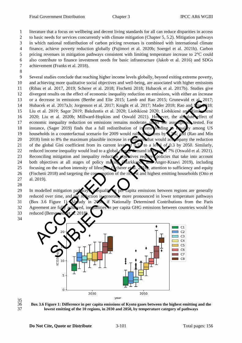
Final Government Distribution Chapter 3 IPCC AR6 WGIII
Do Not Cite, Quote or Distribute 3-101 Total pages: 156
literature that a focus on wellbeing and decent living standards for all can reduce disparities in access 1
to basic needs for services concurrently with climate mitigation (Chapter 5, 5.2). Mitigation pathways 2
in which national redistribution of carbon pricing revenues is combined with international climate 3
finance, achieve poverty reduction globally (Fujimori et al. 2020b; Soergel et al. 2021b). Carbon 4
pricing revenues in mitigation pathways consistent with limiting temperature increase to 2°C could 5
also contribute to finance investment needs for basic infrastructure (Jakob et al. 2016) and SDGs 6
achievement (Franks et al. 2018). 7
8
Several studies conclude that reaching higher income levels globally, beyond exiting extreme poverty, 9
and achieving more qualitative social objectives and well-being, are associated with higher emissions 10
(Ribas et al. 2017, 2019; Scherer et al. 2018; Fischetti 2018; Hubacek et al. 2017b). Studies give 11
divergent results on the effect of economic inequality reduction on emissions, with either an increase 12
or a decrease in emissions (Berthe and Elie 2015; Lamb and Rao 2015; Grunewald et al. 2017; 13
Hubacek et al. 2017a,b; Jorgenson et al. 2017; Knight et al. 2017; Mader 2018; Rao and Min 2018; 14
Liu et al. 2019; Sager 2019; Baležentis et al. 2020; Liobikienė 2020; Liobikienė and Rimkuvienė 15
2020; Liu et al. 2020b; Millward-Hopkins and Oswald 2021). However, the absolute effect of 16
economic inequality reduction on emissions remains moderate, under the assumptions tested. For 17
instance, (Sager 2019) finds that a full redistribution of income leading to equality among US 18
households in a counterfactual scenario for 2009 would raise emissions by 2.3%; and (Rao and Min 19
2018) limit to 8% the maximum plausible increase in emissions that would accompany the reduction 20
of the global Gini coefficient from its current level of 0.55 to a level of 0.3 by 2050. Similarly, 21
reduced income inequality would lead to a global energy demand increase of 7% (Oswald et al. 2021). 22
Reconciling mitigation and inequality reduction objectives requires policies that take into account 23
both objectives at all stages of policy making (Markkanen and Anger-Kraavi 2019), including 24
focusing on the carbon intensity of lifestyles (Scherer et al. 2018), attention to sufficiency and equity 25
(Fischetti 2018) and targeting the consumption of the richest and highest emitting households (Otto et 26
al. 2019). 27
28
In modelled mitigation pathways, inequality in per capita emissions between regions are generally 29
reduced over time, and the reduction is generally more pronounced in lower temperature pathways 30
(Box 3.6 Figure 1). Already in 2030, if Nationally Determined Contributions from the Paris 31
Agreement are fully achieved, inequalities in per capita GHG emissions between countries would be 32
reduced (Benveniste et al. 2018). 33
34
35 Box 3.6 Figure 1: Difference in per capita emissions of Kyoto gases between the highest emitting and the 36
lowest emitting of the 10 regions, in 2030 and 2050, by temperature category of pathways 37
ACCEPTED VERSION
SUBJECT TO FIN
AL EDITS
Final Government Distribution Chapter 3 IPCC AR6 WGIII
Do Not Cite, Quote or Distribute 3-102 Total pages: 156
1
Through avoiding impacts of climate change, which fall more heavily on low-income countries, 2
communities and households and exacerbate poverty, mitigation reduces inequalities and poverty (see 3
section 3.6.4.2). 4
5
END BOX HERE 6
7
The remainder of this section covers specific domains of sustainable development: food (3.7.2), water 8
(3.7.3), energy (3.7.4), health (3.7.5), biodiversity (3.7.6) and multisector - Cities, infrastructure, 9
industry, production & consumption (3.7.7). These represent the areas with the strongest research 10
connecting mitigation to sustainable development. The links to individual SDGs are given within 11
these sections. Each domain covers the benefits of avoided climate impacts and the implications 12
(synergies and trade-offs) of mitigation efforts. 13
14
3.7.2 Food 15
The goal of SDG2 is to achieve “zero-hunger” by 2030. According to the UN (2015), over 25% of the 16
global population currently experience food insecurity and nearly 40% of these experience severe 17
food insecurity, a situation worsened by the covid pandemic (Paslakis et al. 2021). 18
19
3.7.2.1 Benefits of avoided climate impacts along mitigation pathways 20
Climate change will reduce crop yields, increase food insecurity, and negatively influence nutrition 21
and mortality (high confidence) (AR6 WGII Chapter 5). Climate mitigation will thus reduce these 22
impacts, and hence reduce food insecurity (high confidence). The yield reduction of global food 23
production will increase food insecurity and influence nutrition and mortality (Springmann et al. 24
2016a; Hasegawa et al. 2014). For instance, (Springmann et al. 2016a) estimate that climate change 25
could lead to 315,000-736,000 additional deaths by 2050, though these could mostly be averted by 26
stringent mitigation efforts. Reducing warming reduces the impacts of climate change, including 27
extreme climates, on food production and risk of hunger (Hasegawa et al. 2014, 2021b). 28
29
3.7.2.2 Implications of mitigation efforts along pathways 30
Recent studies explore the effect of climate change mitigation on agricultural markets and food 31
security (Hasegawa et al. 2018; Havlík et al. 2014; Fujimori et al. 2019; Doelman et al. 2019). 32
Mitigation policies aimed at achieving 1.5-2°C, if not managed properly, could negatively affect the 33
food security through changes in land and food prices (high confidence), leading to increases in the 34
population at risk of hunger by 80 to 280 million people compared to baseline scenarios. These 35
studies assume uniform carbon prices on AFOLU sectors (with some sectoral caps) and do not 36
account for climate impacts on food production. 37
38
Mitigating climate change while ensuring that food security is not adversely affected requires a range 39
of different strategies and interventions (high confidence). (Fujimori et al. 2018) explore possible 40
economic solutions to these unintended impacts of mitigation (e.g., agricultural subsidies, food aid, 41
and domestic reallocation of income) with an additional small (<0.1%) change in global GDP. 42
Targeted food-security support is needed to shield impoverished and vulnerable people from the risk 43
of hunger that could be caused by the economic effects of policies narrowly focussed on climate 44
objectives. Introducing more biofuels and careful selection of bioenergy feedstocks could also reduce 45
negative impacts (FAO WFP, WHO 2017). Reconciling bioenergy demands with food and 46
biodiversity, as well as competition for land and water, will require changes in food systems – 47
agricultural intensification, open trade, less consumption of animal-products and reduced food losses 48
– and advanced biotechnologies (Henry et al. 2018; Xu et al. 2019). 49
50
ACCEPTED VERSION
SUBJECT TO FIN
AL EDITS
Final Government Distribution Chapter 3 IPCC AR6 WGIII
Do Not Cite, Quote or Distribute 3-103 Total pages: 156
There are many other synergistic measures for climate mitigation and food security. Agricultural 1
technological innovation can improve the efficiency of land use and food systems, thus reducing the 2
pressure on land from increasing food demand (Foley et al. 2011; Humpenöder et al. 2018; Popp et al. 3
2014; Obersteiner et al. 2016; Doelman et al. 2019). Furthermore, decreasing consumption of animal 4
products could contribute to SDG3.4 by reducing the risk of non-communicable diseases (Garnett 5
2016). 6
7
Taken together, climate changes will reduce crop yields, increase food insecurity and influence 8
nutrition and mortality (high confidence) (see 3.7.2.1). However, if measures are not properly 9
designed, mitigating climate change will also negatively impact on food consumption and security. 10
Additional solutions to negative impacts associated with climate mitigation on food production and 11
consumption include a transition to a sustainable agriculture and food system that is less resource 12
intensive, more resilient to a changing climate, and in line with biodiversity and social targets (Kayal 13
et al. 2019). 14
15
3.7.3 Water 16
Water is relevant to SDG 6 (clean water and sanitation), SDG 15 (ecosystem protection and water 17
systems), and SDG Targets 12.4 and 3.9 (water pollution and health). This section discusses water 18
quantity, water quality, and water-related extremes. See 3.7.5 for water-related health effects. 19
20
3.7.3.1 Benefits of avoided climate impacts along mitigation pathways 21
Global precipitation, evapotranspiration, runoff and water availability increase with warming 22
(Hanasaki et al. 2013; Greve et al. 2018) (see also WGII Chapter 4). Climate change also affects the 23
occurrence of and exposure to hydrological extremes (high confidence) (Arnell and Lloyd-Hughes 24
2014; Asadieh and Krakauer 2017; Dottori et al. 2018; IPCC 2019a; Naumann et al. 2018; Do et al. 25
2020) (see also WGII Chapter 4). Climate models project increases in precipitation intensity (high 26
confidence), local flooding (medium confidence), and drought risk (very high confidence) (Arnell and 27
Lloyd-Hughes 2014; Asadieh and Krakauer 2017; Dottori et al. 2018; IPCC 2019a) (see also WGII 28
Chapter 4). 29
30
The effect of climate change on water availability and hydrological extremes varies by region (high 31
confidence) due to differences in the spatial patterns of projected precipitation changes (Hanasaki et 32
al. 2013; Koutroulis et al. 2019; Schewe et al. 2014; Schlosser et al. 2014; Asadieh and Krakauer 33
2017; Dottori et al. 2018; Naumann et al. 2018) (see also WGII Chapter 4). Global exposure to water 34
stress is projected to increase with increased warming, but increases will not occur in all regions 35
(Arnell and Lloyd-Hughes 2014; Gosling and Arnell 2016; Hanasaki et al. 2013; IPCC 2019a; 36
Schewe et al. 2014). 37
38
Limiting warming could reduce water-related risks (high confidence) (O’Neill et al. 2017b; Byers et 39
al. 2018; Hurlbert et al. 2019) (see also WGII Chapter 4) and the population exposed to increased 40
water stress (Arnell and Lloyd-Hughes 2014; Gosling and Arnell 2016; Hanasaki et al. 2013; IPCC 41
2019a; Schewe et al. 2014). 42
43
The effect of climate change on water depends on the climate model, the hydrological model, and the 44
metric (high confidence) stress (Arnell and Lloyd-Hughes 2014; Gosling and Arnell 2016; Hanasaki 45
et al. 2013; IPCC 2019a; Schewe et al. 2014; Schlosser et al. 2014). However, the effect of 46
socioeconomic development could be larger than the effect of climate change (high confidence) 47
(Arnell and Lloyd-Hughes 2014; Schlosser et al. 2014; Graham et al. 2020). 48
49
ACCEPTED VERSION
SUBJECT TO FIN
AL EDITS

Final Government Distribution Chapter 3 IPCC AR6 WGIII
Do Not Cite, Quote or Distribute 3-104 Total pages: 156
Climate change can also affect water quality (both thermal and chemical) (Liu et al. 2017), leading to 1
increases in stream temperature and nitrogen loading in rivers (Ballard et al. 2019). 2
3
3.7.3.2 Implications of mitigation efforts along pathways 4
5
The effect of mitigation on water demand depends on the mitigation technologies deployed (high 6
confidence) (Bonsch et al. 2016; Chaturvedi et al. 2013a,b; Jakob and Steckel 2016; Hejazi et al. 7
2014; Kyle et al. 2013; Fujimori et al. 2017; Maïzi et al. 2017; Mouratiadou et al. 2016; Parkinson et 8
al. 2019; Bijl et al. 2018; Cui et al. 2018; Graham et al. 2018; Hanasaki et al. 2013). Some mitigation 9
options could increase water consumption (volume removed and not returned) while decreasing 10
withdrawals (total volume of water removed, some of which may be returned) (Kyle et al. 2013; 11
Mouratiadou et al. 2016; Fricko et al. 2016; Parkinson et al. 2019). Bioenergy and BECCS can 12
increase water withdrawals and water consumption (high confidence) (Bonsch et al. 2016; Chaturvedi 13
et al. 2013a; Hejazi et al. 2014; Jakob and Steckel 2016; Kyle et al. 2013; Fujimori et al. 2017; Maïzi 14
et al. 2017; Mouratiadou et al. 2016; Parkinson et al. 2019; Yamagata et al. 2018; Séférian et al. 2018) 15
(see also WGII Chapter 4). DACCS (Fuhrman et al. 2020) and CCS (Kyle et al. 2013; Fujimori et al. 16
2017) could increase water demand; however, the implications of CCS depend on the cooling 17
technology and when capture occurs (Magneschi et al. 2017; Maïzi et al. 2017; Giannaris et al. 2020). 18
Demand-side mitigation (e.g., dietary change, reduced food waste, reduced energy demand) can 19
reduce water demand (Bajželj et al. 2014; Aleksandrowicz et al. 2016; Springmann et al. 2018; Green 20
et al. 2018). Introducing specific measures (e.g., environmental flow requirements, improved 21
efficiency, priority rules) can reduce water withdrawals (Bertram et al. 2018; Bijl et al. 2018; 22
Parkinson et al. 2019). 23
24
The effect of mitigation on water quality depends on the mitigation option, its implementation, and 25
the aspect of quality considered (high confidence) (McElwee et al. 2020; Smith et al. 2019; Sinha et 26
al. 2019; Ng et al. 2010; Fuhrman et al. 2020; Flörke et al. 2019; Karlsson et al. 2020). 27
28
3.7.4 Energy 29
Energy is relevant to SDG7 on sustainable and affordable energy access. Access to sufficient levels of 30
reliable, affordable and renewable energy is essential for sustainable development. Currently, over 1 31
billion people still lack access to electricity (Ribas et al. 2019). 32
33
3.7.4.1 Benefits of avoided climate impacts along mitigation pathways 34
Climate change alters the production of energy through changes in temperature (hydropower, fossil 35
fuel, nuclear, solar, bioenergy, transmission and pipelines), precipitation (hydropower, fossil fuel, 36
nuclear, bioenergy), windiness (wind, wave), and cloudiness (solar) (high confidence). Increases in 37
temperature reduce efficiencies of thermal power plants (e.g., fossil fuel and nuclear plants) with air-38
cooled condensers by 0.4-0.7% oC increase in ambient temperature (Cronin et al. 2018a; Yalew, S. G. 39
et al. 2020; Simioni and Schaeffer 2019). Potentials and costs for renewable energy technologies are 40
also affected by climate change, though with considerable regional variation and uncertainty (Gernaat 41
et al. 2021). Biofuel yields could increase or decrease depending on the level of warming, changes in 42
precipitation, and the effect of CO2 fertilization (Calvin et al. 2013; Kyle et al. 2014; Gernaat et al. 43
2021). Coastal energy facilities could potentially be impacted by sea-level rise (Brown et al. 2014). 44
45
The energy sector uses large volumes of water (Fricko et al. 2016), making it highly vulnerable to 46
climate change (Tan and Zhi 2016) (high confidence). Thermoelectric and hydropower sources are the 47
most vulnerable to water stress (van Vliet et al. 2016). Restricted water supply to these power sources 48
can affect grid security and affordable energy access (Koch et al. 2014; Ranzani et al. 2018; Zhang et 49
al. 2018d).The hydropower facilities from high mountain areas of Central Europe, Iceland, Western 50
ACCEPTED VERSION
SUBJECT TO FIN
AL EDITS
Final Government Distribution Chapter 3 IPCC AR6 WGIII
Do Not Cite, Quote or Distribute 3-105 Total pages: 156
US/Canada, and Latin America (Hock et al. 2019) as well as Africa and China (Bartos and Chester 1
2015; Eyer and Wichman 2018; Tarroja et al. 2016; Savelsberg et al. 2018; Ranzani et al. 2018; 2
Zhang et al. 2018d; Conway et al. 2017; Zhou et al. 2018; Gaupp et al. 2015; Wang et al. 2019; Byers 3
et al. 2018) have experienced changes in seasonality and availability. 4
5
3.7.4.2 Implications of mitigation efforts along pathways 6
Extending energy access to all in line with SDG7 is compatible with strong mitigation consistent with 7
the Paris agreement (high confidence). The Low Energy Demand (LED) scenario projects that these 8
twin goals can be achieved by relying heavily on energy efficiency and rapid social transformations 9
(Grubler et al. 2018). The IEA’s Sustainable Development Scenario (IEA 2020a) achieves 10
development outcomes but with higher average energy use, and bottom-up modelling suggests that 11
decent living standards could be provided to all in 2040-2050 with roughly 150 EJ, or 40% of current 12
final energy use (Kikstra et al. 2021b; Millward-Hopkins et al. 2020). The trade-offs between climate 13
mitigation and increasing energy consumption of the world’s poorest are negligible (Rao and Min 14
2018; Scherer et al. 2018). 15
16
The additional energy demand to meet the basic cooling requirement in Global South is estimated to 17
be much larger than the electricity needed to provide basic residential energy services universally via 18
clean and affordable energy, as defined by SDG7 (IEA 2019; Mastrucci et al. 2019) (high 19
confidence). If conventional air conditioning systems are widely deployed to provide cooling, energy 20
use could rise significantly (van Ruijven et al. 2019; Falchetta and Mistry 2021; Bezerra et al. 2021), 21
thus creating a positive feedback further increasing cooling demand. However, the overall emissions 22
are barely altered by the changing energy demand composition with reductions in heating demand 23
occurring simultaneously (Isaac and van Vuuren 2009; Labriet et al. 2015; McFarland et al. 2015; 24
Clarke et al. 2018). Some mitigation scenarios show price increases of clean cooking fuels, slowing 25
the transition to clean cooking fuels (SDG 7.1) and leaving a billion people in 2050 still reliant on 26
solid fuels in South Asia (Cameron et al. 2016). 27
28
In contrast, future energy infrastructure could improve reliability, thus lowering dependence on high-29
carbon, high-air pollution backup diesel generators (Farquharson et al. 2018) that are often used to 30
cope with unreliable power in developing countries (Maruyama Rentschler et al. 2019). There can be 31
significant reliability issues where mini-grids are used to electrify rural areas (Numminen and Lund 32
2019). A stable, sustainable energy transition policy that considers national sustainable development 33
in the short- and long-term is critical in driving a transition to an energy future that addresses the 34
trilemma of energy security, equity, and sustainability (La Viña et al. 2018). 35
36
3.7.5 Health 37
38
SDG 3 aims to ensure healthy lives and promote well-being for all at all ages. Climate change is 39
increasingly causing injuries, illnesses, malnutrition, threats to mental health and well-being, and 40
deaths (see WGII Chapter 7). Mitigation policies and technologies to reduce GHG emissions are often 41
beneficial for human health on a shorter time scale than benefits in terms of slowing climate change 42
(Limaye et al. 2020). The financial value of health benefits from improved air quality alone is 43
projected to exceed the costs of meeting the goals of the Paris Agreement (Markandya et al. 2018). 44
45
3.7.5.1 Benefits of avoided climate impacts along mitigation pathways 46
47
The human health chapter of the WGII contribution to the AR6 concluded that climate change is 48
increasingly affecting a growing number of health outcomes, with negative net impacts at the global 49
scale and positive only in a few limited situations. There are few estimates of economic costs of 50
ACCEPTED VERSION
SUBJECT TO FIN
AL EDITS
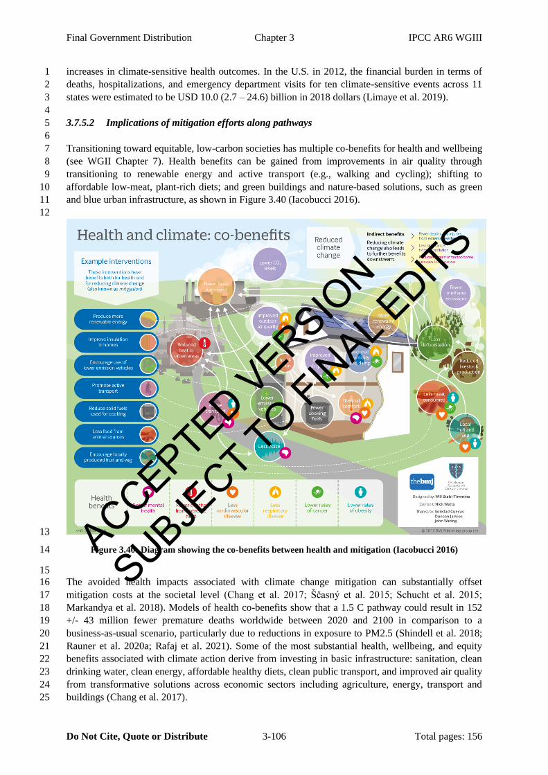
Final Government Distribution Chapter 3 IPCC AR6 WGIII
Do Not Cite, Quote or Distribute 3-106 Total pages: 156
increases in climate-sensitive health outcomes. In the U.S. in 2012, the financial burden in terms of 1
deaths, hospitalizations, and emergency department visits for ten climate-sensitive events across 11 2
states were estimated to be USD 10.0 (2.7 – 24.6) billion in 2018 dollars (Limaye et al. 2019). 3
4
3.7.5.2 Implications of mitigation efforts along pathways 5
6
Transitioning toward equitable, low-carbon societies has multiple co-benefits for health and wellbeing 7
(see WGII Chapter 7). Health benefits can be gained from improvements in air quality through 8
transitioning to renewable energy and active transport (e.g., walking and cycling); shifting to 9
affordable low-meat, plant-rich diets; and green buildings and nature-based solutions, such as green 10
and blue urban infrastructure, as shown in Figure 3.40 (Iacobucci 2016). 11
12
13
Figure 3.40: Diagram showing the co-benefits between health and mitigation (Iacobucci 2016) 14
15
The avoided health impacts associated with climate change mitigation can substantially offset 16
mitigation costs at the societal level (Chang et al. 2017; Ščasný et al. 2015; Schucht et al. 2015; 17
Markandya et al. 2018). Models of health co-benefits show that a 1.5 C pathway could result in 152 18
+/- 43 million fewer premature deaths worldwide between 2020 and 2100 in comparison to a 19
business-as-usual scenario, particularly due to reductions in exposure to PM2.5 (Shindell et al. 2018; 20
Rauner et al. 2020a; Rafaj et al. 2021). Some of the most substantial health, wellbeing, and equity 21
benefits associated with climate action derive from investing in basic infrastructure: sanitation, clean 22
drinking water, clean energy, affordable healthy diets, clean public transport, and improved air quality 23
from transformative solutions across economic sectors including agriculture, energy, transport and 24
buildings (Chang et al. 2017). 25
ACCEPTED VERSION
SUBJECT TO FIN
AL EDITS
Final Government Distribution Chapter 3 IPCC AR6 WGIII
Do Not Cite, Quote or Distribute 3-107 Total pages: 156
1
The health co-benefits of the NDCs for 2040 were compared for two scenarios, one consistent with 2
the goal of the Paris Agreement and the SDGs and the other also placing health as a central focus of 3
the policies (i.e., health in all climate policies scenario) (Hamilton et al. 2021), for Brazil, China, 4
Germany, India, Indonesia, Nigeria, South Africa, the UK, and the USA. Modelling of the energy, 5
food and agriculture, and transport sectors, and associated risk factors related to mortality, suggested 6
the sustainable pathways scenario could result in annual reductions of 1.18 million air pollution-7
related deaths, 5.86 million diet-related deaths, and 1.15 million deaths due to physical inactivity. 8
Adopting the more ambitious health in all climate policies scenario could result in further reductions 9
of 462,000 annual deaths attributable to air pollution, 572,000 annual deaths attributable to diet, and 10
943,000 annual deaths attributable to physical inactivity. These benefits were attributable to the 11
mitigation of direct greenhouse gas emissions and the commensurate actions that reduce exposure to 12
harmful pollutants, as well as improved diets and safe physical activity. 13
14
Cost-benefit analyses for climate mitigation in urban settings that do not account for health may 15
underestimate the potential cost savings and benefits (Hess et al. 2020). The net health benefits of 16
controlling air pollution as part of climate mitigation efforts could reach trillions of dollars annually, 17
depending on the air quality policies adopted globally (Markandya et al. 2018; Scovronick et al. 18
2019b). Air pollution reductions resulting from meeting the Paris Agreement targets were estimated to 19
provide health co-benefits-to-mitigation ratios of between 1.4 and 2.5 (Markandya et al. 2018). In 20
Asia, the benefit of air pollution reduction through mitigation measures were estimated to reduce 21
premature mortality by 0.79 million, with an associated health benefit of USD2.8 trillion versus 22
mitigation costs of USD840 billion, equating to 6% and 2% of GDP, respectively (Xie et al. 2018). 23
Similarly, stabilizing radiative forcing to 3.4 W/m2 in South Korea could cost USD1.3-8.5 billion in 24
2050 and could lead to a USD23.5 billion cost reduction from the combined benefits of avoided 25
premature mortality, health expenditures, and lost work hours (Kim et al. 2020). The health co-26
benefits related to physical exercise and reduced air pollution largely offset the costs of implementing 27
low CO2 emitting urban mobility strategies in three Austrian cities (Wolkinger et al. 2018). 28
29
Just in the United States of America, over the next 50 years, a 2°C pathway could prevent roughly 4.5 30
million premature deaths, about 3.5 million hospitalizations and emergency room visits, and 31
approximately 300 million lost workdays (Shindell 2020). The estimated yearly benefits of USD700 32
billion were more than the estimated cost of the energy transition. 33
34
3.7.6 Biodiversity (land and water) 35
36
Biodiversity covers Life Below Water (SDG 14) and Life On Land (SDG 15). Ecosystem services are 37
relevant to the goals of Zero Hunger (SDG 2), Good Health and Well Being (SDG 3), Clean Water 38
and Sanitation (SDG 6) and Responsible Consumption and Production (SDG 12), as well as being 39
essential to human existence (Díaz et al. 2019). 40
41
3.7.6.1 Benefits of avoided climate impacts along mitigation pathways 42
43
3.7.6.1.1 Terrestrial and freshwater aquatic ecosystems 44
Climate change is a major driver of species extinction and terrestrial and freshwater ecosystems 45
destruction (see WGII Chapter 2) (high confidence). Analysis shows that approximately half of all 46
species with long-term records have shifted their ranges in elevation and about two thirds have 47
advanced their timing of spring events (Parmesan and Hanley 2015). Under 3.2 °C warming, 49% of 48
insects, 44% of plants and 26% of vertebrates are projected to be at risk of extinction. At 2°C, this 49
falls to 18% of insects, 16% of plants and 8% of vertebrates and at 1.5°C, to 6% of insects, 8% of 50
ACCEPTED VERSION
SUBJECT TO FIN
AL EDITS
Final Government Distribution Chapter 3 IPCC AR6 WGIII
Do Not Cite, Quote or Distribute 3-108 Total pages: 156
plants and 4% of vertebrates (Warren et al. 2018). Incidents of migration of invasive species, 1
including pests and diseases, are also attributable to climate change, with negative impacts on food 2
security and vector-borne diseases. Moreover, if climate change reduces crop yields, cropland may 3
expand – a primary driver of biodiversity loss – in order to meet food demand (Molotoks et al. 2020). 4
Land restoration and halting land degradation under all mitigation scenarios has the potential for 5
synergy between mitigation and adaptation. 6
7
3.7.6.1.2 Marine and coastal ecosystems 8
Marine ecosystems are being affected by climate change and growing non-climate pressures including 9
temperature change, acidification, land-sourced pollution, sedimentation, resource extraction and 10
habitat destruction (high confidence) (IPCC 2019b; Bindoff et al. 2019). The impacts of climate 11
drivers and their combinations vary across taxa (WGII Chapter 3). The danger or warming and 12
acidification to coral reefs, rocky shores and kelp forests is well established (high confidence) (WGII 13
Chapter 3). Migration towards optimal thermal and chemical conditions (Burrows et al. 2019) 14
contributes to large scale redistribution of fish and invertebrate populations, and major impacts on 15
global marine biomass production and maximum sustainable yield (Bindoff et al. 2019). 16
17
3.7.6.2 Implications of mitigation efforts along pathways 18
Mitigation measures have the potential to reduce the progress of negative impacts on ecosystems, 19
although it is unlikely that all impacts can be mitigated (high confidence) (Ohashi et al. 2019). The 20
specifics of mitigation achievement are crucial, since large-scale deployment of some climate 21
mitigation and land-based CDR measures could have deleterious impacts on biodiversity (Santangeli 22
et al. 2016; Hof et al. 2018). 23
Climate change mitigation actions to reduce or slow negative impacts on ecosystems are likely to 24
support the achievement of SDGs 2, 3, 6, 12, 14 and 15. Some studies show that stringent and 25
constant GHG mitigation practices bring a net benefit to global biodiversity even if land-based 26
mitigation measures are also adopted (Ohashi et al. 2019), as opposed to delayed action which would 27
require much more widespread use of BECCS. Scenarios based on demand reductions of energy and 28
land-based production are expected to avoid many such consequences, due to their minimized reliance 29
on BECCS (Grubler et al. 2018; Conijn et al. 2018; Bowles et al. 2019; Soergel et al. 2021a). 30
Stringent mitigation that includes reductions in demand for animal-based foods and food-waste could 31
also relieve pressures on land-use and biodiversity (high confidence), both directly by reducing 32
agricultural land requirements (Leclère et al. 2020) and indirectly by reducing the need for land-based 33
CDR (van Vuuren et al. 2018). 34
35
As environmental conservation and sustainable use of the earth’s terrestrial species and ecosystems 36
are strongly related, recent studies have evaluated interconnections among key aspects of land and 37
show pathway to the global sustainable future of land (Erb et al. 2016; Humpenöder et al. 2018; Popp 38
et al. 2014; Obersteiner et al. 2016). Most studies agree that many biophysical options exist to achieve 39
global climate mitigation and sustainable land-use in future. Conserving local biodiversity requires 40
careful policy design in conjunction with land-use regulations and societal transformation in order to 41
minimize the conversion of natural habitats. 42
43
3.7.7 Cities and infrastructure 44
This subsection focuses upon SDG9, Industry, Innovation and Infrastructure and SDG11, Sustainable 45
Cities and Communities. 46
47
3.7.7.1 Benefits of avoided climate impacts along mitigation pathways 48
By 2100, urban population will be almost double and more urban areas will be built (Jiang and 49
O’Neill 2017), although Covid-19 may modify these trends (Kii 2021). Urbanization will amplify 50
ACCEPTED VERSION
SUBJECT TO FIN
AL EDITS

Final Government Distribution Chapter 3 IPCC AR6 WGIII
Do Not Cite, Quote or Distribute 3-109 Total pages: 156
projected air temperature changes in cities, including amplifying heat waves (see WGI Chapter 10, 1
Box 10.3). Benefits of climate mitigation in urban areas include reducing heat, air pollution and 2
flooding. Industrial infrastructure and production-consumption supply networks also benefit from 3
avoided impacts. 4
5
3.7.7.2 Implications of mitigation efforts along pathways 6
Many co-benefits to urban mitigation actions (see Chapter 8, Section 8.2.1) that improve the 7
liveability of cities and contribute to achieving SDG11. In particular, compact, urban form, efficient 8
technologies and infrastructure can play a valuable role in mitigation by reducing energy demand 9
(Güneralp et al. 2017; Creutzig et al. 2016), thus averting carbon lock-in, while reducing land sprawl 10
and hence increasing carbon storage and biodiversity (D’Amour et al. 2017). Benefits of mitigation 11
include air quality improvements from decreased traffic and congestion when private vehicles are 12
displaced by other modes; health benefits from increases in active travel; and lowered urban heat 13
island effects from green-blue infrastructures (section 8.2.1). 14
15
However, increasing urban density or enlarging urban green spaces can increase property prices and 16
reduce affordability (Section 8.2.1). Raising living conditions for slum dwellers & people living in 17
informal settlements will require significant materials and energy; however, regeneration can be 18
conducted in ways that avoid carbon-intense infrastructure lock-in (see Chapter 8 & 9). Cities affect 19
other regions through supply chains (Marinova et al. 2020). 20
21
Sustainable production, consumption and management of natural resources are consistent with, and 22
necessary for, mitigation (Chapters 5 & 11). Demand-side measures can lower requirements for 23
upstream material and energy use (Chapter 5). In terms of industrial production, transformational 24
changes across sectors will be necessary for mitigation (Chapter 11, sections 11.3 and 11.4). 25
26
Addressing multiple SDG arenas requires new systemic thinking in the areas of governance and 27
policy, such as those proposed by (Sachs et al. 2019). 28
29
3.8 Feasibility of socio/techno/economic transitions 30
The objective of this section is to discuss concepts of feasibility in the context of the low carbon 31
transition and pathways. We aim to identify drivers of low carbon scenarios feasibility and to 32
highlight enabling conditions which cam ameliorate feasibility concerns. 33
34
3.8.1 Feasibility frameworks for the low carbon transition and scenarios 35
Effectively responding to climate change and achieving sustainable development requires overcoming 36
a series of challenges to transition away from fossil-based economies. Feasibility can be defined in 37
many ways (see also Chapter 1). The political science literature (Majone 1975a,b; Gilabert and 38
Lawford-Smith 2012) distinguishes the feasibility of ‘what’ (i.e. emission reduction strategies),’when 39
and where” (i.e. in the year 2050, globally) and “whom” (i.e. cities). It distinguishes desirability from 40
political feasibility (von Stechow et al. 2015): the former represents a normative assessments of the 41
compatibility with societal goals (i.e. SDGs) while the latter evaluate the plausibility of what can be 42
attained given the prevailing context of transformation (Nielsen et al. 2020). Feasibility concerns are 43
context and time dependent and malleable: enabling conditions can help overcome them. For 44
example, public support for carbon taxes has been hard to secure but appropriate policy design and 45
household rebates can help dissipate opposition (Carattini et al. 2019; Murray and Rivers 2015). 46
47
Regarding scenarios, the feasibility ‘what’ question is the one most commonly dealt with in the 48
literature, though most of the studies have focused on expanding low carbon system, and yet political 49
ACCEPTED VERSION
SUBJECT TO FIN
AL EDITS
Final Government Distribution Chapter 3 IPCC AR6 WGIII
Do Not Cite, Quote or Distribute 3-110 Total pages: 156
constraints might arise mostly from phasing out fossil fuel-based ones (Spencer et al. 2018; Fattouh et 1
al. 2019). The ‘when and where’ dimension can also be related to the scenario assessment, but only 2
insofar the models generating them can differentiate time and geographical contextual factors. 3
Distinguishing mitigation potential by regional institutional capacity has a significant influence on the 4
costs of stabilizing climate (Iyer et al. 2015c). The ‘whom’ question is the most difficult to capture by 5
scenarios, given the multitude of actors involved as well as their complex interactions. The focus of 6
socio-technical transition sciences on the co-evolutionary processes can shed light on the dynamics of 7
feasibility (Nielsen et al. 2020). 8
9
The when-where-whom distinction allows depicting a feasibility frontier beyond which 10
implementation challenges prevent mitigation action (Jewell and Cherp 2020). Even if the current 11
feasibility frontier appears restraining in some jurisdictions, it is context-dependent and dynamic as 12
innovation proceeds and institutional capacity builds up (Nielsen et al. 2020). The question is whether 13
the feasibility frontier can move faster than the pace at which the carbon budget is being exhausted. 14
Jewell et al. (2019) show that the emission savings from the pledges of premature retirement of coal 15
plants is 150 times less than globally committed emissions from existing coal power plants. The 16
pledges come from countries with high institutional capacity and relatively low shares of coal in 17
electricity. Other factors currently limiting the capacity to steer transitions at the necessary speed 18
include the electoral market orientation of politicians (Willis 2017), the status quo orientation of 19
senior public officials (Geden 2016), path dependencies created by 'instrument constituencies' (Béland 20
and Howlett 2016), or the benefits of deliberate inconsistencies between talk, decisions and actions in 21
climate policy (Rickards et al. 2014). All in all, a number of different delay mechanisms in both 22
science and policy have been identified to potentially impede climate goal achievement (Karlsson and 23
Gilek 2020) - see also Chapter 13. 24
25
In addition to its contextual and dynamic nature, feasibility is a multi-dimensional concept. The IPCC 26
1.5°C special report distinguishes 6 dimensions of feasibility: geophysical, environmental-ecological, 27
technological, economic, socio-cultural and institutional. At the individual option level, different 28
mitigation strategies face various barriers as well as enablers (see Chapter 6 for the option-level 29
assessment). However, a systemic transformation involves interconnections of a wide range of 30
indicators. Model-based assessments are meant to capture the integrative elements of the transition 31
and of associated feasibility challenges. However, the translation of model-generated pathways into 32
feasibility concerns (Rogelj et al. 2018b) has developed only recently. Furthermore, multiple forms of 33
knowledge can be mobilized to support strategic decision-making and complement scenario analysis 34
(Turnheim and Nykvist 2019). We discuss both approaches next. 35
36
3.8.2 Feasibility appraisal of low carbon scenarios 37
Evaluating the feasibility of low carbon pathways can take different forms. In the narrowest sense, 38
there is feasibility pertaining the reporting of model-generated scenarios: here an infeasible scenario is 39
one which cannot meet the constraints embedded implicitly or explicitly in the models which 40
attempted to generate it. Second, there is a feasibility that relates to specific elements or overall 41
structure characterizing the low carbon transition compared to some specified benchmark. 42
43
3.8.2.1 Model solvability 44
In order to be generated, scenarios must be coherent with the constraints and assumptions embedded 45
in the models (i.e., deployment potential of given technologies, physical and geological limits) and in 46
the scenario design (i.e., carbon budget). Sometimes, models cannot solve specific scenarios. This 47
provides a first, coarse indication of feasibility concerns. Specific vetting criteria can be imposed, 48
such as carbon price values above which scenarios should not be reported, as in Clarke et al. (2009). 49
However, model solvability raises issues of aggregation in model ensemble. Since model solving is 50
ACCEPTED VERSION
SUBJECT TO FIN
AL EDITS
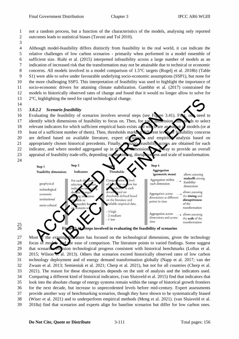
Final Government Distribution Chapter 3 IPCC AR6 WGIII
Do Not Cite, Quote or Distribute 3-111 Total pages: 156
not a random process, but a function of the characteristics of the models, analysing only reported 1
outcomes leads to statistical biases (Tavoni and Tol 2010). 2
3
Although model-feasibility differs distinctly from feasibility in the real world, it can indicate the 4
relative challenges of low carbon scenarios - primarily when performed in a model ensemble of 5
sufficient size. Riahi et al. (2015) interpreted infeasibility across a large number of models as an 6
indication of increased risk that the transformation may not be attainable due to technical or economic 7
concerns. All models involved in a model comparison of 1.5°C targets (Rogelj et al. 2018b) (Table 8
S1) were able to solve under favourable underlying socio-economic assumptions (SSP1), but none for 9
the more challenging SSP3. This interpretation of feasibility was used to highlight the importance of 10
socio-economic drivers for attaining climate stabilization. Gambhir et al. (2017) constrained the 11
models to historically observed rates of change and found that it would no longer allow to solve for 12
2°C, highlighting the need for rapid technological change. 13
14
3.8.2.2 Scenario feasibility 15
Evaluating the feasibility of scenarios involves several steps (see Figure 3.41). First, one need to 16
identify which dimensions of feasibility to focus on. Then, for each dimension, one needs to select 17
relevant indicators for which sufficient empirical basis exists and which are an output of models (or at 18
least of a sufficient number of them). Then, thresholds marking different levels of feasibility concerns 19
are defined based on available literature, expert elicitations and empirical analysis based on 20
appropriately chosen historical precedents. Finally, scenario feasibility scores are obtained for each 21
indicator, and where needed aggregated up in time or dimensions, as a way to provide an overall 22
appraisal of feasibility trade-offs, depending on the timing, disruptiveness and scale of transformation. 23
24
25 Figure 3.41: Steps involved in evaluating the feasibility of scenarios 26
Most of the existing literature has focused on the technological dimensions, given the technology 27
focus of models and the ease of comparison. The literature points to varied findings. Some suggest 28
that scenarios envision technological progress consistent with historical benchmarks (Loftus et al. 29
2015; Wilson et al. 2013). Others that scenarios exceed historically observed rates of low carbon 30
technology deployment and of energy demand transformation globally (Napp et al. 2017; van der 31
Zwaan et al. 2013; Semieniuk et al. 2021; Cherp et al. 2021), but not for all countries (Cherp et al. 32
2021). The reason for these discrepancies depends on the unit of analysis and the indicators used. 33
Comparing a different kind of historical indicators, (van Sluisveld et al. 2015) find that indicators that 34
look into the absolute change of energy systems remain within the range of historical growth frontiers 35
for the next decade, but increase to unprecedented levels before mid-century. Expert assessments 36
provide another way of benchmarking scenarios, though they have shown to be systematically biased 37
(Wiser et al. 2021) and to underperform empirical methods (Meng et al. 2021). (van Sluisveld et al. 38
2018a) find that scenarios and experts align for baseline scenarios but differ for low carbon ones. 39
ACCEPTED VERSION
SUBJECT TO FIN
AL EDITS

Final Government Distribution Chapter 3 IPCC AR6 WGIII
Do Not Cite, Quote or Distribute 3-112 Total pages: 156
Scenarios rely more on conventional technologies based on existing infrastructure (such as nuclear 1
and CCS) than what forecasted by experts. Overall, the technology assessment of the feasibility space 2
highlights that Paris-compliant transformations would have few precedents, but not zero (Cherp et al. 3
2021). 4
5
Recent approaches have addressed multiple dimensions of feasibility, an important advancement since 6
social and institutional aspects are as if not more important than technology ones (Jewell and Cherp 7
2020). Feasibility corridors of scenarios based on their scale, rate of change and disruptiveness have 8
been identified (Kriegler et al. 2018b; Warszawski et al. 2021). The reality check shows that many 9
1.5°C compatible scenarios violate the feasibility corridors. The ones which didn’t are associated with 10
a greater coverage of the available mitigation levers (Warszawski et al. 2021). 11
12
Brutschin et al. (2021) proposed an operational framework covering all six dimensions of feasibility. 13
They developed a set of multi-dimensional metrics capturing the timing, disruptiveness and the scale 14
of the transformative change within each dimension (as in Kriegler et al. (2018b)). Thresholds of 15
feasibility risks of different intensity are obtained through the review of the relevant literature and 16
empirical analysis of historical data. Novel indicators include governance levels (Andrijevic et al. 17
2020a). The 17 bottom-up indicators are then aggregated up across time and dimension, as way to 18
highlight feasibility trade-offs. Aggregation is done via compensatory approaches such as the 19
geometric mean. This is employed, for instance, for the Human Development Index. A conceptual 20
example of this approach as applied to the IPCC AR6 scenarios database is shown in Figure 3.42 and 21
further described in the Annex. 22
23
24 Figure 3.42: Example of multi-dimensional feasibility analysis and indicators used in the IPCC AR6 25 scenarios. The approach defines relevant indicators characterizing the key dimensions of feasibility. 26 Indicators capture the timing, scale and disruptiveness challenges. Low, medium and high feasibility 27 concerns are defined based on historical trends and available literature. Details about indicator and 28
thresholds values can be found in Annex III 29
In Figure 3.43, we show the results of applying the methodology of Brutschin et al. (2021) to the AR6 30
scenarios database. The charts highlight the dynamic nature of feasibility risks, which are mostly 31
concentrated in the decades before mid-century except for geophysical risks driven by CO2 removals 32
ACCEPTED VERSION
SUBJECT TO FIN
AL EDITS

Final Government Distribution Chapter 3 IPCC AR6 WGIII
Do Not Cite, Quote or Distribute 3-113 Total pages: 156
later in the century. Different dimensions pose differentiated challenges: for example, institutional 1
feasibility challenges appear to be the most relevant, in line with the qualitative literature. Thus, 2
feasibility concerns might be particularly relevant in countries with weaker institutional capacity. The 3
Figure also highlights the key role of policy and technology, as enabling factors. In particular (Panel 4
B), internationally coordinated and immediate emission reductions allow to smooth out feasibility 5
concerns and reduce long term challenges compared to delayed policy action, as a result of a more 6
gradual transition and lower requirements of CO2 removals. For the same climate objective, different 7
illustrative mitigation pathways entail somewhat different degrees and distributions of implementation 8
challenges (panel C). 9
10
ACCEPTED VERSION
SUBJECT TO FIN
AL EDITS

Final Government Distribution Chapter 3 IPCC AR6 WGIII
Do Not Cite, Quote or Distribute 3-114 Total pages: 156
Figure 3.43: Feasibility characteristics of the Paris-consistent scenarios in AR6 scenarios database, 1 applying the methodology by : Feasibility corridors for the AR6 scenarios database, applying the 2
methodology by (Brutschin et al. 2021). Panel A: the fraction of scenarios falling within 3 categories of 3 feasibility concerns (Plausible, Best Case, Unprecedented), for different times (2030, 2050, 2100), different 4 climate categories consistent with the Paris Agreement and five dimensions. Panel B: composite feasibility 5 score (obtained by geometric mean of underlying indicators) over time for scenarios with immediate and 6 delayed global mitigation efforts, for different climate categories (C1-C2-C3. Note: no C1 scenarios has 7
delayed participation). Panel C: Fraction of scenarios which in any point in time over the century exceed 8 the feasibility concerns, for C1 and C3 climate categories. Overlayed are the Illustrative Mitigation 9
Pathways (LP, SP, Ren: C1 category; Neg, GS: C3 category) 10
3.8.3 Feasibility in the light of socio-technical transitions 11
The limitations associated with quantitative low-carbon transition pathways stem from a predominant 12
reliance on techno-economic considerations with a simplified or non-existent representation of the 13
socio-political and institutional agreement. Accompanying the required deployment of low carbon 14
technologies will be the formation of new socio-technical systems (Bergek et al. 2008). With a socio-15
technical system being defined as a cluster of elements comprising of technology, regulation, user 16
practices and markets, cultural meaning, infrastructure, maintenance networks, and supply networks 17
(Geels and Geels 2005; Hofman et al. 2004); the interrelationship between technological systems and 18
social systems must be comprehensively understood. It is of vital importance that the pro-cess of 19
technical change must considered in its institutional and social context so as to ascertain potential 20
transition barriers which in turn provide an indication of pathway feasibility. In order to address the 21
multitudinous challenges associated with low-carbon transition feasibility and governance, it has been 22
opined that the robustness of evaluating pathways may be improved by the bridging of differing 23
quantitative-qualitative analytical approaches (Haxeltine et al. 2008; Foxon et al. 2010; Hughes 2013; 24
Wangel et al. 2013; Li et al. 2015; Turnheim et al. 2015; Geels et al. 2016a,b, 2018; Moallemi et al. 25
2017; De Cian et al. 2018; Li and Strachan 2019). The rationale for such analytical bridging is to 26
rectify the issue that in isolation each disciplinary approach only can generate a fragmented 27
comprehension of the transition pathway with the consequence being an incomplete identification of 28
associated challenges in terms of feasibility. Concerning low-carbon transition pathways generated by 29
IAMs, it has been argued that a comprehensive analysis should include social scientific enquiry 30
(Geels et al. 2016a, 2018; van Sluisveld et al. 2018b). The normative analysis of IAM pathways 31
assists in the generation of a vision or the formulation of a general plan with this being complemented 32
by socio-technical transition theory (Geels et al. 2016a). Such an approach thereby allowing for the 33
socio-political feasibility and the social acceptance and legitimacy of low-carbon options to be 34
considered. Combining computer models and the multi-level perspective can help identify ‘transition 35
bottlenecks’ (Geels et al. 2018). Similarly, increased resolution of integrated assessment models’ 36
actors has led to more realistic narratives of transition in terms of granularity and behaviour 37
(McCollum et al. 2017; van Sluisveld et al. 2018b). Increased data availability of actual behaviour 38
from smart technology lowers the barriers to representing behavioural change in computer 39
simulations, and thus better represent crucial demand side transformations (Creutzig et al. 2018). 40
Increasing the model resolution is a meaningful way forward. However, integrating a much broader 41
combination of real-life aspects and dynamics into models could lead to an increased complexity that 42
could restrict them to smaller fields of applications (De Cian et al. 2018). 43
44
Other elements of feasibility relate to social justice, which could be essential to enhance the political 45
and public acceptability of the low carbon transition. Reviewing the literature, one study finds that 46
employing social justice as an orienting principle can increase the political feasibility of low carbon 47
policies (Patterson et al. 2018). Three elements are identified as key: i) protecting vulnerable people 48
from climate change impacts, ii), protecting people from disruptions of transformation, iii), enhancing 49
the process of envisioning and implementing an equitable post-carbon society. 50
51
ACCEPTED VERSION
SUBJECT TO FIN
AL EDITS
Final Government Distribution Chapter 3 IPCC AR6 WGIII
Do Not Cite, Quote or Distribute 3-115 Total pages: 156
3.8.4 Enabling factors 1
There is strong agreement that the climate policy institutional framework as well as technological 2
progress have a profound impact on the attainability of low carbon pathways. Delaying international 3
cooperation reduces the available carbon budget and locks into carbon intensive infrastructure 4
exacerbating implementation challenges (Clarke et al. 2009; Bosetti et al. 2009; Krey and Riahi 2009; 5
Boucher et al. 2009; Keppo and Rao 2007; van Vliet et al. 2009; Knopf et al. 2011; Luderer et al. 6
2013; Jakob et al. 2012; Aboumahboub et al. 2014; Bertram et al. 2021; Popp et al. 2014; Rogelj et al. 7
2013a; Riahi et al. 2015; Kriegler et al. 2014a; Gambhir et al. 2017). Similarly, technological 8
availability influences the feasibility of climate stabilization, though differently for different 9
technologies (Iyer et al. 2015a; Kriegler et al. 2014a; Riahi et al. 2015). 10
11
One of the most relevant factors affecting mitigation pathways and their feasibility is the rate and kind 12
of socio-economic development. For example, certain socio-economic trends and assumptions 13
about policy effectiveness preclude achieving stringent mitigation futures (Rogelj et al. 2018b). 14
The risk of failure increases markedly in high growth, unequal and/or energy-intensive worlds -15
such as those characterized by the shared socio-economic pathways SSP3, SSP4 and SSP5. On the 16
other hand, socio-economic development conducive to mitigation relieves the energy sector 17
transformation from relying on large scale technology development: for example, the amount of 18
biomass with CCS in SSP1 is one third of that in SSP5. The reason why socio-economic trends matter 19
so much is that they both affect the CO2 emissions in counterfactual scenarios as well as the 20
mitigation capacity (Riahi et al. 2017; Rogelj et al. 2018b). Economic growth assumptions are the 21
most important determinant of scenario emissions (Marangoni et al. 2017). De- and post-growth 22
scenarios have been suggested as valuable alternatives to be considered (Hickel et al. 2021; Keyßer 23
and Lenzen 2021), though substantial challenges remain regarding political feasibility (Keyßer and 24
Lenzen 2021). 25
26
The type of policy instrument assumed to drive the decarbonization process also play a vital role for 27
determining feasibility. The majority of scenarios exploring climate stabilization pathways in the past 28
have focused on uniform carbon pricing as the most efficient instrument to regulate emissions. 29
However, carbon taxation raises political challenges (Beiser-McGrath and Bernauer 2019), see also 30
Chapter 13 and 14. Carbon pricing will transfer economic surplus from consumers and producers to 31
the government. Losses for producers will be highly concentrated in those industries possessing fixed 32
or durable assets with “high asset specificity” (Murphy 2002; Dolphin et al. 2020). These sectors have 33
opposed climate jurisdictions (Jenkins 2014). Citizens are sensitive to rising energy prices, though 34
revenue recycling can be used to increase support (Carattini et al. 2019). A recent model comparison 35
project confirms findings from the extant literature: using revenues to reduce pre-existing capital or, 36
to a lesser extent, labour taxes, reduces policy costs and eases distributional concerns (Mcfarland et al. 37
2018; Barron et al. 2018). 38
39
Nonetheless, winning support will require a mix of policies which go beyond carbon pricing, and 40
include subsidies, mandates and feebates (Rozenberg et al. 2018; Jenkins 2014). More recent 41
scenarios take into account a more comprehensive range of policies and regional heterogeneity in the 42
near to medium term (Roelfsema et al. 2020). Regulatory policies complementing carbon prices could 43
reduce the implementation challenges by increasing short term emission reduction, though they could 44
eventually reduce economic efficiency (Bertram et al. 2015b; Kriegler et al. 2018a). Innovation 45
policies such as subsidies to R&D have been shown to be desirable due to innovation market failures, 46
and also address the dynamic nature of political feasibility (Bosetti et al. 2011). 47
48
ACCEPTED VERSION
SUBJECT TO FIN
AL EDITS

Final Government Distribution Chapter 3 IPCC AR6 WGIII
Do Not Cite, Quote or Distribute 3-116 Total pages: 156
3.9 Methods of assessment and gaps in knowledge and data 1
3.9.1 AR6 mitigation pathways 2
The analysis in this chapter relies on the available literature as well as an assessment of the scenarios 3
contained in the AR6 scenarios database. Scenarios were submitted by research and other institutions 4
following an open call (see Annex III Part II). The scenarios included in the AR6 scenarios database 5
are an unstructured ensemble, as they are from multiple underlying studies and depend on which 6
institutions chose to submit scenarios to the database. As noted in Section 3.2, they do not represent 7
the full scenario literature or the complete set of possible scenarios. For example, scenarios that 8
include climate change impacts or economic degrowth are not fully represented, as these scenarios, 9
with a few exceptions, were not submitted to the database. Additionally, sensitivity studies, which 10
could help elucidate model behaviour and drivers of change, are mostly absent from the database - 11
though examples exist in the literature (Marangoni et al. 2017). 12
13
The AR6 scenarios database contains 3131 scenarios of which 2425 with global scope were 14
considered by this chapter, generated by almost 100 different model versions, from more than 50 15
model families. Of the 1686 vetted scenarios, 1202 provided sufficient information for a climate 16
categorization. Around 46% of the pathways are consistent with an end of century temperature of at 17
least likely limiting warming to below 2°C. There are many ways of constructing scenarios that limit 18
warming to a particular level and the choice of scenario construction has implications for the timing 19
of both net zero CO2 and GHG emissions and the deployment of CDR (Emmerling et al. 2019; Rogelj 20
et al. 2019b; Johansson et al. 2020). The AR6 scenarios database includes scenarios where 21
temperature is temporarily exceeded (40% of all scenarios in the database have median temperature in 22
2100 that is 0.1C lower than median peak temperature). Climate stabilization scenarios are typically 23
implemented by assuming a carbon price rising at a particular rate per year, though that rate varies 24
across model, scenario, and time period. Standard scenarios assume a global single carbon price to 25
minimize policy costs. Cost minimizing pathways can be reconciled with equity considerations 26
through posterior international transfers. Many scenarios extrapolate current policies and include non-27
market, regulatory instruments such as technology mandates. 28
29
Scenarios are not independent of each other and not representative of all possible outcomes, nor of the 30
underlying scenario generation process; thus, the statistical power of the database is limited. 31
Dependencies in the data generation process originate from various sources. Certain model groups, 32
and types, are over-represented. For example, 8 model teams contributed with 90% of scenarios. 33
Second, not all models can generate all scenarios, and these differences are not random, thereby 34
creating selection bias (Tavoni and Tol 2010). Third, there are strong model dependencies: the 35
modelling scientific community shares code and data, and several IAMs are open source. 36
37
3.9.2 Models assessed in this chapter 38
The models assessed in this chapter differ in their sectoral coverage and the level of complexity in 39
each sector. Models tend to have more detail in their representation of energy supply and 40
transportation, than they do for industry (Section 3.4; Annex III). Some models include detailed land 41
use models, while others exclude land models entirely and use supply curves to represent bioenergy 42
potential (Bauer et al. 2018a). IAMs do not include all mitigation options available in the literature 43
(Rogelj et al. 2018b; Smith et al. 2019). For example, most IAM pathways exclude many granular 44
demand-side mitigation options and land-based mitigation options found in more detailed sectoral 45
models; additionally, only a few pathways include CDR options beyond afforestation/reforestation 46
and BECCS. Section 3.4 and Chapter 12 include some results and comparisons to non-IAM models 47
(e.g., bottom-up studies and detailed sectoral models). These sectoral studies often include a more 48
complete set of mitigation options but exclude feedbacks and linkages across sectors which may alter 49
ACCEPTED VERSION
SUBJECT TO FIN
AL EDITS
Final Government Distribution Chapter 3 IPCC AR6 WGIII
Do Not Cite, Quote or Distribute 3-117 Total pages: 156
the mitigation potential of a given sector. There is an increasing focus in IAM studies on SDGs 1
(Section 3.7), with some studies reporting the implications of mitigation pathways on SDGs (e.g., 2
Bennich et al. (2020)) and others using achieving SDGs as a constraint on the scenario itself (van 3
Vuuren et al. 2015; Soergel et al. 2021a). However, IAMs are still limited in the SDGs they represent, 4
often focusing on energy, water, air pollution and land. On the economic side, the majority of the 5
models report information on marginal costs (i.e., carbon price). Only a subset provides full economic 6
implications measured by either economic activity or welfare. Also often missing, is detail about 7
economic inequality within countries or large aggregate regions. 8
9
For further details about the models and scenarios, see Annex III. 10
11
12
Frequently Asked Questions (FAQs) 13
FAQ 3.1 – Is it possible to stabilize warming without net negative CO2 and GHG emissions? 14
Yes. Achieving net zero CO2 emissions and sustaining them into the future is sufficient to stabilize 15
the CO2-induced warming signal which scales with the cumulative net amount of CO2 emissions. At 16
the same time, the warming signal of non-CO2 GHGs can be stabilized or reduced by declining 17
emissions that lead to stable or slightly declining concentrations in the atmosphere. For short-lived 18
GHGs with atmospheric lifetimes of less than 20 years, this is achieved when residual emissions are 19
reduced to levels that are lower than the natural removal of these gases in the atmosphere. Taken 20
together, mitigation pathways that bring CO2 emissions to net zero and sustain it, while strongly 21
reducing non-CO2 GHGs to levels that stabilize or decline their aggregate warming contribution, will 22
stabilize warming without using net negative CO2 emissions and with positive overall GHG emissions 23
when aggregated using GWP100. A considerable fraction of pathways limiting warming to 1.5°C 24
with no or limited overshoot and likely limiting warming to 2°C, respectively, do not or only 25
marginally (<10 GtCO2 cumulative until 2100) deploy net negative CO2 emissions (26% and 46%, 26
respectively) and do not reach net zero GHG emissions by the end of the century (48% and 70%, 27
respectively). This is no longer the case in pathways that return warming to 1.5°C after a high 28
overshoot (typically > 0.1°C). All of these pathways deploy net negative emissions on the order of 29
330 (26-623 GtCO2) (median and 5th-95th percentile) and 87% achieve net negative GHGs emissions 30
in AR6 GWP-100 before the end of the century. Hence, global net negative CO2 emissions, and net 31
zero or net negative GHG emissions, are only needed to decline, not to stabilize global warming. The 32
deployment of carbon dioxide removal (CDR) is distinct from the deployment of net negative CO2 33
emissions, because it is also used to neutralize residual CO2 emissions to achieve and sustain net zero 34
CO2 emissions. CDR deployment can be considerable in pathways without net negative emissions and 35
all pathways limiting warming to 1.5°C use it to some extent. 36
37
FAQ 3.2 – How can net zero emissions be achieved and what are the implications of net zero 38
emissions for the climate? 39
Halting global warming in the long term requires, at a minimum, that no additional CO2 emissions 40
from human activities are added to the atmosphere (i.e., CO2 emissions must reach “net” zero). Given 41
that CO2 emissions constitute the dominant human influence on global climate, global net zero CO2 42
emissions are a prerequisite for stabilizing warming at any level. However, CO2 is not the only 43
greenhouse gas that contributes to global warming and reducing emissions of other greenhouse gases 44
alongside CO2 towards net zero emissions of all GHGs would lower the level at which global 45
temperature would peak. The temperature implications of net zero GHG emissions depend on the 46
bundle of gases that is being considered, and the emissions metric used to calculate aggregated GHG 47
emissions and removals. If reached and sustained, global net zero GHG emissions using the 100-year 48
Global Warming Potential (GWP-100) will lead to gradually declining global temperature. 49
ACCEPTED VERSION
SUBJECT TO FIN
AL EDITS
Final Government Distribution Chapter 3 IPCC AR6 WGIII
Do Not Cite, Quote or Distribute 3-118 Total pages: 156
Not all emissions can be avoided. Achieving net zero CO2 emissions globally therefore requires deep 1
emissions cuts across all sectors and regions, along with active removal of CO2 from the atmosphere 2
to balance remaining emissions that may be too difficult, too costly or impossible to abate at that time. 3
Achieving global net zero GHG emissions would require, in addition, deep reductions of non-CO2 4
emissions and additional CO2 removals to balance remaining non-CO2 emissions. 5
Not all regions and sectors must reach net zero CO2 or GHG emissions individually to achieve global 6
net zero CO2 or GHG emissions, respectively; instead, positive emissions in one sector or region can 7
be compensated by net negative emissions from another sector or region. The time each sector or 8
region reaches net zero CO2 or GHG emissions depends on the mitigation options available, the cost 9
of those options, and the policies implemented (including any consideration of equity or fairness). 10
Most modelled pathways that likely limit warming to 2°C above pre-industrial levels and below use 11
land-based CO2 removal such as afforestation/reforestation and BECCS to achieve net zero CO2 and 12
net zero GHG emissions even while some CO2 and non-CO2 emissions continue to occur. Pathways 13
with more demand-side interventions that limit the amount of energy we use, or where the diet that we 14
consume is changed, can achieve net zero CO2, or net zero GHG emissions with less carbon dioxide 15
removal. All available studies require at least some kind of carbon dioxide removal to reach net zero; 16
that is, there are no studies where absolute zero GHG or even CO2 emissions are reached by deep 17
emissions reductions alone. 18
Total GHG emissions are greater than emissions of CO2 only; reaching net zero CO2 emissions 19
therefore occurs earlier, by up to several decades, than net zero GHG emissions in all modelled 20
pathways. In most modelled pathways that likely limit warming to 2°C above pre-industrial levels and 21
below in the most cost-effective way, the AFOLU and energy supply sectors reach net zero CO2 22
emissions several decades earlier than other sectors; however, many pathways show much reduced, 23
but still positive net GHG emissions in the AFOLU sector in 2100. 24
25
FAQ 3.3 – How plausible are high emissions scenarios, and how do they inform policy? 26
IAMs are used to develop a wide range of scenarios describing future trajectories for greenhouse gas 27
emissions based on a wide set of assumptions regarding socio-economic development, technological 28
changes, political development and climate policy. Typically, the IAM-based scenarios can be divided 29
into a) reference scenarios (describing possible trajectories in the absence of new stringent climate 30
policies) and b) mitigation scenarios (describing the impact of various climate policy assumptions). 31
Reference scenarios typically result in high emissions and, subsequently, high levels of climate 32
change (in the order of 2.5-4 °C during the 21st century). The purpose of such reference scenarios is 33
to explore the consequences of climate change and act as a reference for mitigation scenarios. The 34
possible emission levels for reference scenarios diverge from stabilising and even slowly declining 35
emissions (e.g., for current policy scenarios or SSP1) to very high emission levels (e.g., SSP5 and 36
RCP8.5). The latter leads to nearly 5 °C of warming by the end of the century for medium climate 37
sensitivity. Hausfather and Peters (2020) pointed out that since 2011, the rapid development of 38
renewable energy technologies and emerging climate policy have made it considerably less likely that 39
emissions could end up as high as RCP8.5. This means that reaching emissions levels as high as 40
RCP8.5 has become less likely. Still, high emissions cannot be ruled out for many reasons, including 41
political factors and, for instance, higher than anticipated population and economic growth. Climate 42
projections of RCP8.5 can also result from strong feedbacks of climate change on (natural) emission 43
sources and high climate sensitivity (see WGI Chapter 7). Therefore, their median climate impacts 44
might also materialise while following a lower emission path (e.g., Hausfather and Betts (2020)). All-45
in-all, this means that high-end scenarios have become considerably less likely since AR5 but cannot 46
be ruled out. High-end scenarios (like RCP8.5) can be very useful to explore high-end risks of climate 47
change but are not typical ‘business-as-usual” projections and should therefore not be presented as 48
such. 49
50
ACCEPTED VERSION
SUBJECT TO FIN
AL EDITS
Final Government Distribution Chapter 3 IPCC AR6 WGIII
Do Not Cite, Quote or Distribute 3-119 Total pages: 156
References 1
Abel, G. J., B. Barakat, S. KC, and W. Lutz, 2016: Meeting the Sustainable Development Goals leads 2
to lower world population growth. Proc. Natl. Acad. Sci., 113(50), 14294 LP – 14299, 3
doi:10.1073/pnas.1611386113. 4
Aboumahboub, T. et al., 2014: On the regional distribution of climate mitigation costs: the impact of 5
delayed cooperative action. Clim. Chang. Econ., 5(1), 1–27, doi:10.1142/S2010007814400028. 6
Acemoglu, D., P. Aghion, L. Bursztyn, and D. Hemous, 2012: The Environment and Directed 7
Technical Change. Am Econ Rev, 102(1), 131–166, doi:10.1257/aer.102.1.131. 8
Acemoglu, D., U. Akcigit, D. Hanley, and W. Kerr, 2016: Transition to clean technology. J. Polit. 9
Econ., 124(1), 52–104, doi:10.1086/684511. 10
Adler, M. et al., 2017: Priority for the worse-off and the social cost of carbon. Nat. Clim. Chang., 11
7(6), 443–449, doi:10.1038/nclimate3298. 12
Aghion, P., C. Hepburn, A. Teytelboym, and D. Zenghelis, 2019: Path dependence, innovation and 13
the economics of climate change. In: Handbook on Green Growth, Edward Elgar Publishing, 14
Cheltenham, UK, pp. 67–83. 15
Akimoto, K., F. Sano, J. Oda, H. Kanaboshi, and Y. Nakano, 2021: Climate change mitigation 16
measures for global net-zero emissions and the roles of CO2 capture and utilization and direct 17
air capture. Energy Clim. Chang., 2, 100057, doi:https://doi.org/10.1016/j.egycc.2021.100057. 18
Aldy, J. et al., 2016: Economic tools to promote transparency and comparability in the Paris 19
Agreement. Nat. Clim. Chang., 6(11), 1000–1004, doi:10.1038/nclimate3106. 20
Aleksandrowicz, L., R. Green, E. J. M. Joy, P. Smith, and A. Haines, 2016: The Impacts of Dietary 21
Change on Greenhouse Gas Emissions, Land Use, Water Use, and Health: A Systematic 22
Review. PLoS One, 11(11), e0165797. 23
Allen, M. R. et al., 2009: Warming caused by cumulative carbon emissions towards the trillionth 24
tonne. Nature, 458(7242), 1163–1166, doi:10.1038/nature08019. 25
Allen, M. R. et al., 2016: New use of global warming potentials to compare cumulative and short-26
lived climate pollutants. Nat. Clim. Chang., 6(8), 773–776, doi:10.1038/nclimate2998. 27
Allen, M. R. et al., 2018: Framing and Context Coordinating. In: Global Warming of 1.5°C. An IPCC 28
Special Report on the impacts of global warming of 1.5°C above pre-industrial levels and 29
related global greenhouse gas emission pathways, in the context of strengthening the global 30
response to the threat of climate change, pp. 49–91. 31
Anderegg, W. R. L. et al., 2020: Climate-driven risks to the climate mitigation potential of forests. 32
Science, 368(6497), eaaz7005, doi:10.1126/science.aaz7005. 33
Anderson, K., and A. Larkin, 2013: Avoiding dangerous climate change demands de-growth 34
strategies from wealthier nations. https://kevinanderson.info/blog/avoiding-dangerous-climate-35
change-demands-de-growth-strategies-from-wealthier-nations/. 36
Anderson, K., and G. Peters, 2016: The trouble with negative emissions. Science, 354(6309), 182–37
183, doi:10.1126/science.aah4567. 38
Andrijevic, M., J. Crespo Cuaresma, R. Muttarak, and C.-F. Schleussner, 2020a: Governance in 39
socioeconomic pathways and its role for future adaptive capacity. Nat. Sustain., 3(1), 35–41, 40
doi:10.1038/s41893-019-0405-0. 41
Andrijevic, M., C.-F. Schleussner, M. J. Gidden, D. L. McCollum, and J. Rogelj, 2020b: COVID-19 42
recovery funds dwarf clean energy investment needs. Science, 370(6514), 298–300, 43
doi:10.1126/science.abc9697. 44
Arinoa, Y. et al., 2016: Estimating option values of solar radiation management assuming that climate 45
sensitivity is uncertain. Proc. Natl. Acad. Sci. U. S. A., 113(21), 5886–5891, 46
doi:10.1073/pnas.1520795113. 47
Arnell, N. W., and B. Lloyd-Hughes, 2014: The global-scale impacts of climate change on water 48
resources and flooding under new climate and socio-economic scenarios. Clim. Change, 122(1–49
2), 127–140, doi:10.1007/s10584-013-0948-4. 50
Arvesen, A., G. Luderer, M. Pehl, B. L. Bodirsky, and E. G. Hertwich, 2018: Deriving life cycle 51
assessment coefficients for application in integrated assessment modelling. Environ. Model. 52
Softw., 99, 111–125, doi:https://doi.org/10.1016/j.envsoft.2017.09.010. 53
ACCEPTED VERSION
SUBJECT TO FIN
AL EDITS

Final Government Distribution Chapter 3 IPCC AR6 WGIII
Do Not Cite, Quote or Distribute 3-120 Total pages: 156
Asadieh, B., and N. Y. Krakauer, 2017: Global change in streamflow extremes under climate change 1
over the 21st century. Hydrol. Earth Syst. Sci., 21(11), 5863–5874, doi:10.5194/hess-21-5863-2
2017. 3
Auffhammer, M., P. Baylis, and C. H. Hausman, 2017: Climate change is projected to have severe 4
impacts on the frequency and intensity of peak electricity demand across the United States. 5
Proc. Natl. Acad. Sci. U. S. A., 114(8), 1886–1891, doi:10.1073/pnas.1613193114. 6
Azevedo, I., C. Bataille, J. Bistline, L. Clarke, and S. Davis, 2021: Net-Zero Emissions Energy 7
Systems: What We Know and Do Not Know. Energy Clim. Chang., , 100049. 8
Babacan, O. et al., 2020: Assessing the feasibility of carbon dioxide mitigation options in terms of 9
energy usage. Nat. Energy, 5(9), 720–728, doi:10.1038/s41560-020-0646-1. 10
Bajželj, B., and K. S. Richards, 2014: The positive feedback loop between the impacts of climate 11
change and agricultural expansion and relocation. Land, 3(3), 898–916, 12
doi:10.3390/land3030898. 13
Bajželj, B. et al., 2014: Importance of food-demand management for climate mitigation. Nat. Clim. 14
Chang., 4(10), 924–929, doi:10.1038/nclimate2353. 15
Baker, J. S., C. M. Wade, B. L. Sohngen, S. Ohrel, and A. A. Fawcett, 2019: Potential 16
complementarity between forest carbon sequestration incentives and biomass energy expansion. 17
Energy Policy, 126(August 2018), 391–401, doi:10.1016/j.enpol.2018.10.009. 18
Baležentis, T., G. Liobikienė, D. Štreimikienė, and K. Sun, 2020: The impact of income inequality on 19
consumption-based greenhouse gas emissions at the global level: {A} partially linear approach. 20
J. Environ. Manage., 267, 110635, doi:10.1016/j.jenvman.2020.110635. 21
Ballard, T. C., E. Sinha, and A. M. Michalak, 2019: Long-Term Changes in Precipitation and 22
Temperature Have Already Impacted Nitrogen Loading. Environ. Sci. Technol., 53(9), 5080–23
5090, doi:10.1021/acs.est.8b06898. 24
Barker, T., E. Alexandri, J. F. Mercure, Y. Ogawa, and H. Pollitt, 2016: GDP and employment effects 25
of policies to close the 2020 emissions gap. Clim. Policy, 16(4), 393–414, 26
doi:10.1080/14693062.2014.1003774. 27
Barron, A. R., A. A. Fawcett, M. A. C. Hafstead, J. R. Mcfarland, and A. C. Morris, 2018: POLICY 28
INSIGHTS FROM THE EMF 32 STUDY ON U.S. CARBON TAX SCENARIOS. Clim. 29
Chang. Econ., 09(01), 1840003, doi:10.1142/S2010007818400031. 30
Bartos, M. D., and M. V. Chester, 2015: Impacts of climate change on electric power supply in the 31
Western United States. Nat. Clim. Chang., 5(8), 748–752, doi:10.1038/nclimate2648. 32
Bastien-Olvera, B. A., and F. C. Moore, 2020: Use and non-use value of nature and the social cost of 33
carbon. Nat. Sustain., , 1–8, doi:10.1038/s41893-020-00615-0. 34
Battiston, S., A. Mandel, I. Monasterolo, F. Schütze, and G. Visentin, 2017: A climate stress-test of 35
the financial system. Nat. Clim. Chang., 7(4), 283–288, doi:10.1038/nclimate3255. 36
Battiston, S., I. Monasterolo, K. Riahi, and B. J. van Ruijven, 2021: Accounting for finance is key for 37
climate mitigation pathways. Science, 372(6545), 918–920, doi:10.1126/science.abf3877. 38
Bauer, N. et al., 2017: Shared Socio-Economic Pathways of the Energy Sector – Quantifying the 39
Narratives. Glob. Environ. Chang., 42, doi:10.1016/j.gloenvcha.2016.07.006. 40
Bauer, N. et al., 2018a: Global energy sector emission reductions and bioenergy use: overview of the 41
bioenergy demand phase of the EMF-33 model comparison. Clim. Change, , 42
doi:10.1007/s10584-018-2226-y. 43
Bauer, N., C. McGlade, J. Hilaire, and P. Ekins, 2018b: Divestment prevails over the green paradox 44
when anticipating strong future climate policies. Nat. Clim. Chang., 8(2), 130–134, 45
doi:10.1038/s41558-017-0053-1. 46
Bauer, N. et al., 2020: Quantification of an efficiency–sovereignty trade-off in climate policy. Nature, 47
588(7837), 261–266, doi:10.1038/s41586-020-2982-5. 48
Beach, R. H. et al., 2015: Climate change impacts on US agriculture and forestry: Benefits of global 49
climate stabilization. Environ. Res. Lett., 10(9), doi:10.1088/1748-9326/10/9/095004. 50
Beck, S., and M. Mahony, 2017: The IPCC and the politics of anticipation. Nat. Clim. Chang., 7(5), 51
311–313, doi:10.1038/nclimate3264. 52
Beck, S., and M. Mahony, 2018: The politics of anticipation: The IPCC and the negative emissions 53
technologies experience. Glob. Sustain., 1, 1–8, doi:10.1017/sus.2018.7. 54
Bednar, J. et al., 2021: Operationalizing the net-negative carbon economy. Nature, , 55
ACCEPTED VERSION
SUBJECT TO FIN
AL EDITS

Final Government Distribution Chapter 3 IPCC AR6 WGIII
Do Not Cite, Quote or Distribute 3-121 Total pages: 156
doi:10.1038/s41586-021-03723-9. 1
Beiser-McGrath, L. F., and T. Bernauer, 2019: Could revenue recycling make effective carbon 2
taxation politically feasible? Sci. Adv., 5(9), eaax3323, doi:10.1126/sciadv.aax3323. 3
Belaia, M., J. B. Moreno-Cruz, and D. W. Keith, 2021: Optimal Climate Policy in 3D: Mitigation, 4
Carbon Removal and Solar Geoengineering. Clim. Chang. Econ., , 2150008, 5
doi:10.1142/S2010007821500081. 6
Béland, D., and M. Howlett, 2016: How Solutions Chase Problems: Instrument Constituencies in the 7
Policy Process. Governance, 29(3), 393–409, doi:https://doi.org/10.1111/gove.12179. 8
Bennich, T., N. Weitz, and H. Carlsen, 2020: Deciphering the scientific literature on SDG 9
interactions: A review and reading guide. Sci. Total Environ., 728, 138405, 10
doi:10.1016/j.scitotenv.2020.138405. 11
Benveniste, H., O. Boucher, C. Guivarch, H. Le Treut, and P. Criqui, 2018: Impacts of nationally 12
determined contributions on 2030 global greenhouse gas emissions: uncertainty analysis and 13
distribution of emissions. Environ. Res. Lett., 13(1), 14022, doi:10.1088/1748-9326/aaa0b9. 14
Benveniste, H., J. C. Cuaresma, M. Gidden, and R. Muttarak, 2021: Tracing international migration in 15
projections of income and inequality across the Shared Socioeconomic Pathways. Clim. Change, 16
166(3), 39, doi:10.1007/s10584-021-03133-w. 17
Bergek, A., S. Jacobsson, and B. A. Sandén, 2008: ‘Legitimation’ and ‘development of positive 18
externalities’: two key processes in the formation phase of technological innovation systems. 19
Technol. Anal. Strateg. Manag., 20(5), 575–592, doi:10.1080/09537320802292768. 20
Berger, A. et al., 2017: How much can nuclear energy do about global warming? Int. J. Glob. Energy 21
Issues, 40(1/2), doi:10.1504/IJGEI.2017.080766. 22
Berthe, A., and L. Elie, 2015: Mechanisms explaining the impact of economic inequality on 23
environmental deterioration. Ecol. Econ., 116, 191–200, doi:10.1016/j.ecolecon.2015.04.026. 24
Bertram, C. et al., 2015a: Carbon lock-in through capital stock inertia associated with weak near-term 25
climate policies. Technol. Forecast. Soc. Change, 90(PA), 62–72, 26
doi:10.1016/j.techfore.2013.10.001. 27
Bertram, C. et al., 2015b: Complementing carbon prices with technology policies to keep climate 28
targets within reach. Nat. Clim. Chang., 5(3), 235–239, doi:10.1038/nclimate2514. 29
Bertram, C. et al., 2018: Targeted policies can compensate most of the increased sustainability risks in 30
1.5 °c mitigation scenarios. Environ. Res. Lett., 13(6), doi:10.1088/1748-9326/aac3ec. 31
Bertram, C. et al., 2021: Energy system developments and investments in the decisive decade for the 32
Paris Agreement goals. Environ. Res. Lett., 16(7), 74020, doi:10.1088/1748-9326/ac09ae. 33
Bezerra, P. et al., 2021: Impacts of a warmer world on space cooling demand in Brazilian households. 34
Energy Build., 234, 110696, doi:https://doi.org/10.1016/j.enbuild.2020.110696. 35
Bibas, R., A. Méjean, and M. Hamdi-Cherif, 2015: Energy efficiency policies and the timing of 36
action: An assessment of climate mitigation costs. Technol. Forecast. Soc. Change, 90(PA), 37
137–152, doi:10.1016/j.techfore.2014.05.003. 38
Bijl, D. L. et al., 2018: A Global Analysis of Future Water Deficit Based On Different Allocation 39
Mechanisms. Water Resour. Res., 54(8), 5803–5824, doi:10.1029/2017WR021688. 40
Bindoff, N., W. Cheung, J. Kairo, V. Arístegui, and R. Guinder, 2019: Changing ocean, marine 41
ecosystems, and dependent communities. 42
Bistline, J., M. Budolfson, and B. Francis, 2020: Deepening transparency about value-laden 43
assumptions in energy and environmental modelling: improving best practices for both 44
modellers and non-modellers. Clim. Policy, , 1–15, doi:10.1080/14693062.2020.1781048. 45
Bistline, J. E. T., and G. J. Blanford, 2021: Impact of carbon dioxide removal technologies on deep 46
decarbonization of the electric power sector. Nat. Commun., 12(1), 3732, doi:10.1038/s41467-47
021-23554-6. 48
Blanford, G. J., E. Kriegler, and M. Tavoni, 2014: Harmonization vs. fragmentation: Overview of 49
climate policy scenarios in EMF27. Clim. Change, 123(3–4), 383–396, doi:10.1007/s10584-50
013-0951-9. 51
Böhringer, C., E. J. Balistreri, and T. F. Rutherford, 2012: The role of border carbon adjustment in 52
unilateral climate policy: Overview of an Energy Modeling Forum study (EMF 29). Energy 53
Econ., 34, S97–S110. 54
Böhringer, C., K. E. Rosendahl, and H. B. Storrøsten, 2017: Robust policies to mitigate carbon 55
ACCEPTED VERSION
SUBJECT TO FIN
AL EDITS

Final Government Distribution Chapter 3 IPCC AR6 WGIII
Do Not Cite, Quote or Distribute 3-122 Total pages: 156
leakage. J. Public Econ., 149, 35–46, doi:https://doi.org/10.1016/j.jpubeco.2017.03.006. 1
Böhringer, C., S. Peterson, T. F. Rutherford, J. Schneider, and M. Winkler, 2021: Climate policies 2
after Paris: Pledge, Trade and Recycle: Insights from the 36th Energy Modeling Forum Study 3
(EMF36). Energy Econ., 103, 105471, doi:https://doi.org/10.1016/j.eneco.2021.105471. 4
Bonsch, M. et al., 2016: Trade-offs between land and water requirements for large-scale bioenergy 5
production. GCB Bioenergy, 8(1), 11–24, doi:10.1111/gcbb.12226. 6
Bosetti, V., C. Carraro, and M. Tavoni, 2009: Climate change mitigation strategies in fast-growing 7
countries: The benefits of early action. Energy Econ., 31(SUPPL. 2), S144–S151, 8
doi:10.1016/j.eneco.2009.06.011. 9
Bosetti, V., C. Carraro, R. Duval, and M. Tavoni, 2011: What should we expect from innovation? A 10
model-based assessment of the environmental and mitigation cost implications of climate-related 11
R&D. Energy Econ., 33(6), 1313–1320, doi:10.1016/j.eneco.2011.02.010. 12
Bosetti, V. et al., 2015: Sensitivity to energy technology costs: A multi-model comparison analysis. 13
Energy Policy, 80, 244–263, doi:https://doi.org/10.1016/j.enpol.2014.12.012. 14
Boucher, O., J. A. Lowe, and C. D. Jones, 2009: Implications of delayed actions in addressing carbon 15
dioxide emission reduction in the context of geo-engineering. Clim. Change, 92(3–4), 261–273, 16
doi:10.1007/s10584-008-9489-7. 17
Bowen, A., K. Kuralbayeva, and E. L. Tipoe, 2018: Characterising green employment: {The} impacts 18
of ‘greening’ on workforce composition. Energy Econ., 72, 263–275, 19
doi:10.1016/j.eneco.2018.03.015. 20
Bowles, N., S. Alexander, and M. Hadjikakou, 2019: The livestock sector and planetary boundaries: 21
A ‘limits to growth’ perspective with dietary implications. Ecol. Econ., 160(January), 128–136, 22
doi:10.1016/j.ecolecon.2019.01.033. 23
Boysen, L. R., W. Lucht, D. Gerten, and V. Heck, 2016: Impacts devalue the potential of large-scale 24
terrestrial CO2 removal through biomass plantations. Environ. Res. Lett., 11(9), 1–10, 25
doi:10.1088/1748-9326/11/9/095010. 26
Boysen, L. R. et al., 2017: The limits to global-warming mitigation by terrestrial carbon removal. 27
Earth’s Futur., 5(5), 463–474, doi:10.1002/2016EF000469. 28
BP, 2021: Statistical Review of World Energy 2021. Statistical Review of World Energy, 29
30
Brandi, C., 2015: Safeguarding the earth system as a priority for sustainable development and global 31
ethics: The need for an earth system SDG. J. Glob. Ethics, 11(1), 32–36, 32
doi:10.1080/17449626.2015.1006791. 33
Breyer, C., and M. Jefferson, 2020: Use and Abuse of Energy and Climate Scenarios—A Week of 34
Controversy on Scenarios. Econ. Energy Environ. Policy, 9, doi:10.5547/2160-5890.9.1.mjef. 35
Brockway, P. E., S. Sorrell, G. Semieniuk, M. K. Heun, and V. Court, 2021: Energy efficiency and 36
economy-wide rebound effects: A review of the evidence and its implications. Renew. Sustain. 37
Energy Rev., 141(December 2020), 110781, doi:10.1016/j.rser.2021.110781. 38
Brook, B. W., T. Blees, T. M. L. Wigley, and S. Hong, 2018: Silver Buckshot or Bullet: Is a Future 39
“Energy Mix” Necessary? Sustain. , 10(2), doi:10.3390/su10020302. 40
Brown, C., P. Alexander, A. Arneth, I. Holman, and M. Rounsevell, 2019: Achievement of Paris 41
climate goals unlikely due to time lags in the land system. Nat. Clim. Chang., 9(3), 203–208, 42
doi:10.1038/s41558-019-0400-5. 43
Brown, P. T., and H. Saunders, 2020: Approximate calculations of the net economic impact of global 44
warming mitigation targets under heightened damage estimates. PLoS One, 15(10), e0239520, 45
doi:10.1371/journal.pone.0239520. 46
Brown, P. T., J. Moreno-Cruz, and K. Caldeira, 2020: Break-even year: a concept for understanding 47
intergenerational trade-offs in climate change mitigation policy. Environ. Res. Commun., 2(9), 48
95002, doi:10.1088/2515-7620/abb413. 49
Brown, S., S. Hanson, and R. Nicholls, 2014: Implications of sea-level rise and extreme events around 50
Europe: A review of coastal energy infrastructure. Clim. Change, 122, doi:10.1007/s10584-013-51
0996-9. 52
Brutschin, E. et al., 2021: A multidimensional feasibility evaluation of low-carbon scenarios. Environ. 53
Res. Lett., 16(6), 64069, doi:10.1088/1748-9326/abf0ce. 54
Budolfson, M., F. Dennig, M. Fleurbaey, A. Siebert, and R. H. Socolow, 2017: The comparative 55
ACCEPTED VERSION
SUBJECT TO FIN
AL EDITS

Final Government Distribution Chapter 3 IPCC AR6 WGIII
Do Not Cite, Quote or Distribute 3-123 Total pages: 156
importance for optimal climate policy of discounting, inequalities and catastrophes. Clim. 1
Change, 145(3–4), 481–494, doi:10.1007/s10584-017-2094-x. 2
Budolfson, M. B. et al., 2021: Utilitarian benchmarks for emissions and pledges promote equity, 3
climate and development. Nat. Clim. Chang., 11(10), 827–833, doi:10.1038/s41558-021-01130-4
6. 5
Burgess, M. G., J. Ritchie, J. Shapland, and R. Pielke, 2020: IPCC baseline scenarios have over-6
projected CO2emissions and economic growth. Environ. Res. Lett., 16(1), doi:10.1088/1748-7
9326/abcdd2. 8
Burke, M., W. M. Davis, and N. S. Diffenbaugh, 2018: Large potential reduction in economic 9
damages under UN mitigation targets. Nature, 557(7706), 549–553, doi:10.1038/s41586-018-10
0071-9. 11
Burrows, M. T. et al., 2019: Ocean community warming responses explained by thermal affinities and 12
temperature gradients. Nat. Clim. Chang., 9(12), 959–963, doi:10.1038/s41558-019-0631-5. 13
Butnar, I. et al., 2020: A deep dive into the modelling assumptions for biomass with carbon capture 14
and storage (BECCS): A transparency exercise. Environ. Res. Lett., 15(8), doi:10.1088/1748-15
9326/ab5c3e. 16
Byers, E. et al., 2018: Global exposure and vulnerability to multi-sector development and climate 17
change hotspots. Environ. Res. Lett., 13(5), 055012, doi:10.1088/1748-9326/aabf45. 18
Cai, Y., and T. S. Lontzek, 2019: The Social Cost of Carbon with Economic and Climate Risks. J. 19
Polit. Econ., 127(6), 2684–2734, doi:10.1086/701890. 20
Cai, Y., K. L. Judd, T. M. Lenton, T. S. Lontzek, and D. Narita, 2015: Environmental tipping points 21
significantly affect the cost-benefit assessment of climate policies. Proc. Natl. Acad. Sci. U. S. 22
A., 112(15), 4606–4611, doi:10.1073/pnas.1503890112. 23
Cai, Y., T. M. Lenton, and T. S. Lontzek, 2016: Risk of multiple interacting tipping points should 24
encourage rapid CO2 emission reduction. Nat. Clim. Chang., 6(5), 520–525, 25
doi:10.1038/nclimate2964. 26
Cain, M. et al., 2019: Improved calculation of warming-equivalent emissions for short-lived climate 27
pollutants. npj Clim. Atmos. Sci., 2(1), doi:10.1038/s41612-019-0086-4. 28
Caldecott, B., 2017: Introduction to special issue: stranded assets and the environment. J. Sustain. 29
Financ. Invest., 7(1), 1–13, doi:10.1080/20430795.2016.1266748. 30
Calvin, K. et al., 2013: Implications of simultaneously mitigating and adapting to climate change: 31
Initial experiments using GCAM. Clim. Change, 117(3), 545–560, doi:10.1007/s10584-012-32
0650-y. 33
Calvin, K. et al., 2014a: EU 20-20-20 energy policy as a model for global climate mitigation. Clim. 34
Policy, 14(5), 581–598, doi:10.1080/14693062.2013.879794. 35
Calvin, K. et al., 2014b: Trade-offs of different land and bioenergy policies on the path to achieving 36
climate targets. Clim. Change, 123(3–4), 691–704, doi:10.1007/s10584-013-0897-y. 37
Calvin, K. et al., 2021: Bioenergy for climate change mitigation: Scale and sustainability. GCB 38
Bioenergy, 13(9), 1346–1371, doi:https://doi.org/10.1111/gcbb.12863. 39
Calvin, K. V., R. Beach, A. Gurgel, M. Labriet, and A. M. Loboguerrero Rodriguez, 2014c: 40
Agriculture, forestry, and other land-use emissions in Latin America. Energy Econ., 56, 615–41
624, doi:10.1016/j.eneco.2015.03.020. 42
Cameron, C. et al., 2016: Policy trade-offs between climate mitigation and clean cook-stove access in 43
South Asia. Nat. Energy, 1(1), 1–5, doi:10.1038/nenergy.2015.10. 44
Canadell, J. G., and P. M. S. Monteiro, 2019: Global Carbon and other Biogeochemical Cycles and 45
Feedbacks. In Climate Change 2021: The Physical Science Basis. Contribution of Working 46
Group I to the Sixth Assessment Report of the Intergovernmental Panel on Climate Change 47
[Masson-Delmotte, V., P. Zhai, A. Pirani, S.L. Connors, C. Péan, S. Berger, N. Caud, Y. Chen, 48
L. Goldfarb, M.I. Gomis, M. Huang, K. Leitzell, E. Lonnoy, J.B.R. Matthews, T.K. Maycock, T. 49
Waterfield, O. Yelekçi, R. Yu, and B. Zhou (eds.)]. Cambridge University Press. In Press. . 50
Carattini, S., S. Kallbekken, and A. Orlov, 2019: How to win public support for a global carbon tax. 51
Nature, 565, 289–291. 52
Carton, W., 2019: Carbon Unicorns and Fossil Futures: Whose Emissions Reduction Pathways Is the 53
IPCC Performing? In: Has It Come to This? The Promises and Perils of Geoengineering on the 54
Brink? 55
ACCEPTED VERSION
SUBJECT TO FIN
AL EDITS

Final Government Distribution Chapter 3 IPCC AR6 WGIII
Do Not Cite, Quote or Distribute 3-124 Total pages: 156
Chakravarty, S., and M. Tavoni, 2013: Energy poverty alleviation and climate change mitigation: Is 1
there a trade off? Energy Econ., 40, S67–S73, doi:10.1016/j.eneco.2013.09.022. 2
Chang, K. M. et al., 2017: Ancillary health effects of climate mitigation scenarios as drivers of policy 3
uptake: a review of air quality, transportation and diet co-benefits modeling studies. Environ. 4
Res. Lett., 12(11), 113001, doi:10.1088/1748-9326/aa8f7b. 5
Chateau, J., and A. Saint-Martin, 2013: Economic and employment impacts of climate change 6
mitigation policies in {OECD}: {A} general-equilibrium perspective. Int. Econ., 135–136, 79–7
103, doi:10.1016/j.inteco.2013.08.001. 8
Chaturvedi, V. et al., 2013a: Climate Policy Implications for Agricultural Water Demand. 9
Chaturvedi, V. et al., 2013b: Climate mitigation policy implications for global irrigation water 10
demand. Mitig. Adapt. Strateg. Glob. Chang., 20(3), 389–407, doi:10.1007/s11027-013-9497-4. 11
Chen, C., and M. Tavoni, 2013: Direct air capture of CO2 and climate stabilization: A model based 12
assessment. Clim. Change, 118(1), 59–72, doi:10.1007/s10584-013-0714-7. 13
Cherp, A., V. Vinichenko, J. Jewell, E. Brutschin, and B. Sovacool, 2018: Integrating techno-14
economic, socio-technical and political perspectives on national energy transitions: A meta-15
theoretical framework. Energy Res. Soc. Sci., 37(January 2017), 175–190, 16
doi:10.1016/j.erss.2017.09.015. 17
Cherp, A., V. Vinichenko, J. Tosun, J. A. Gordon, and J. Jewell, 2021: National growth dynamics of 18
wind and solar power compared to the growth required for global climate targets. Nat. Energy, 19
6(7), 742–754, doi:10.1038/s41560-021-00863-0. 20
Cherubini, F., R. M. Bright, and A. H. Strømman, 2013: Erratum: Global climate impacts of forest 21
bioenergy: What, when and how to measure? (Environmental Research Letters (2013) 8 22
(014049)). Environ. Res. Lett., 8(2), doi:10.1088/1748-9326/8/2/029503. 23
Christensen, P., K. Gillingham, and W. Nordhaus, 2018: Uncertainty in forecasts of long-run 24
economic growth. Proc. Natl. Acad. Sci. U. S. A., 115(21), 5409–5414, 25
doi:10.1073/pnas.1713628115. 26
Clarke, L. et al., 2009: International climate policy architectures: Overview of the EMF 22 27
International Scenarios. Energy Econ., 31(SUPPL. 2), S64–S81, 28
doi:10.1016/j.eneco.2009.10.013. 29
Clarke, L. et al., 2018: Effects of long-term climate change on global building energy expenditures. 30
Energy Econ., 72, 667–677, doi:10.1016/j.eneco.2018.01.003. 31
Clarke, L. E. et al., 2014: Assessing transformation pathways. In: Climate Change 2014: Mitigation of 32
Climate Change. Contribution of Working Group III to the Fifth Assessment Report of the 33
Intergovernmental Panel on Climate Change [Edenhofer, O., R.P.-M., S. Y. Sokona, E. 34
Farahani, S. Kadner, K. Seyboth, A. Adler, I. Baum, S. Brunner, P. Eickemeier, B. Kriemann, J. 35
Savolainen, and T.Z. and J.C.M. (eds. . Schlömer, C. von Stechow, (eds.)], Cambridge 36
University Press, Cambridge, United Kingdom and New York, NY, USA. 37
Cointe, B., C. Cassen, and A. Nadaï, 2019: Organising policy-relevant knowledge for climate action: 38
Integrated assessment modelling, the IPCC, and the emergence of a collective expertise on 39
socioeconomic emission scenarios. Sci. Technol. Stud., 32(4), 36–57, doi:10.23987/sts.65031. 40
Colelli, F. Pietro, and E. De Cian, 2020: Cooling demand in integrated assessment models: a 41
methodological review. Environ. Res. Lett., 15(11), 113005, doi:10.1088/1748-9326/abb90a. 42
Collins, M. et al., 2013: Long-term Climate Change: Projections, Commitments and Irreversibility. In: 43
Climate Change 2013: The Physical Science Basis. Contribution of Working Group I to the Fifth 44
Assessment Report of the Intergovernmental Panel on Climate Change [Stocker, T.F. et al., 45
(eds.)], Cambridge University Press, Cambridge, United Kingdom and New York, NY, USA, 46
pp. 1029–1136. 47
Collins, W. J. et al., 2018: Increased importance of methane reduction for a 1.5 degree target. 48
Environ. Res. Lett., 13(5), 54003, doi:10.1088/1748-9326/aab89c. 49
Conijn, J. G., P. S. Bindraban, J. J. Schröder, and R. E. E. Jongschaap, 2018: Can our global food 50
system meet food demand within planetary boundaries? Agric. Ecosyst. Environ., 251(December 51
2016), 244–256, doi:10.1016/j.agee.2017.06.001. 52
Conway, D., C. Dalin, W. A. Landman, and T. J. Osborn, 2017: Hydropower plans in eastern and 53
southern Africa increase risk of concurrent climate-related electricity supply disruption. Nat. 54
Energy, 2(12), 946–953, doi:10.1038/s41560-017-0037-4. 55
ACCEPTED VERSION
SUBJECT TO FIN
AL EDITS
Final Government Distribution Chapter 3 IPCC AR6 WGIII
Do Not Cite, Quote or Distribute 3-125 Total pages: 156
Cosbey, A., S. Droege, C. Fischer, and C. Munnings, 2019: Developing Guidance for Implementing 1
Border Carbon Adjustments: Lessons, Cautions, and Research Needs from the 2
Literature. Rev. Environ. Econ. Policy, 13(1), 3–22, doi:10.1093/reep/rey020. 3
Cowie, A. L. et al., 2021: Applying a science-based systems perspective to dispel misconceptions 4
about climate effects of forest bioenergy. GCB Bioenergy, 13(8), 1210–1231, 5
doi:https://doi.org/10.1111/gcbb.12844. 6
7
Crippa, M., E. et al., 2021: Fossil CO2 and GHG emissions of all world countries - 2021 Report. Joint 8
Research Centre. Ispra. Italy. 9
10
Creutzig, F. et al., 2016: Beyond Technology: Demand-Side Solutions for Climate Change Mitigation. 11
Annu. Rev. Environ. Resour., 41(1), 173–198, doi:10.1146/annurev-environ-110615-085428. 12
Creutzig, F. et al., 2017: The underestimated potential of solar energy to mitigate climate change. 2, 13
17140. 14
Creutzig, F. et al., 2018: Towards demand-side solutions for mitigating climate change. Nat. Clim. 15
Chang., 8(4), 268–271, doi:10.1038/s41558-018-0121-1. 16
Creutzig, F. et al., 2019: The mutual dependence of negative emission technologies and energy 17
systems. Energy Environ. Sci., 12(6), 1805–1817, doi:10.1039/c8ee03682a. 18
Cronin, J., G. Anandarajah, and O. Dessens, 2018a: Climate change impacts on the energy system: a 19
review of trends and gaps. Clim. Change, 151(2), 79–93, doi:10.1007/s10584-018-2265-4. 20
Cronin, J. A., D. Fullerton, and S. Sexton, 2018b: Vertical and Horizontal Redistributions from a 21
Carbon Tax and Rebate. J. Assoc. Environ. Resour. Econ., 6(S1), S169–S208, 22
doi:10.1086/701191. 23
Cui, R. Y. et al., 2018: Regional responses to future, demand-driven water scarcity. Environ. Res. 24
Lett., 13(9), 94006, doi:10.1088/1748-9326/aad8f7. 25
Cui, R. Y. et al., 2019: Quantifying operational lifetimes for coal power plants under the Paris goals. 26
Nat. Commun., 10(1), doi:10.1038/s41467-019-12618-3. 27
D’Alessandro, S., A. Cieplinski, T. Distefano, and K. Dittmer, 2020: Feasible alternatives to green 28
growth. Nat. Sustain., , 1–7, doi:10.1038/s41893-020-0484-y. 29
D’Amour, C. B. et al., 2017: Future urban land expansion and implications for global croplands. Proc. 30
Natl. Acad. Sci. U. S. A., 114(34), 8939–8944, doi:10.1073/pnas.1606036114. 31
Dagnachew, A. G. et al., 2020: Integrating energy access, efficiency and renewable energy policies in 32
Sub-Saharan Africa: a model-based analysis. Environ. Res. Lett., , doi:10.1088/1748-33
9326/abcbb9. 34
Daioglou, V., B. J. van Ruijven, and D. P. van Vuuren, 2012: Model projections for household energy 35
use in developing countries. Energy, 37(1), 601–615, doi:10.1016/j.energy.2011.10.044. 36
Daioglou, V. et al., 2014: Energy demand and emissions of the non-energy sector. Energy Environ. 37
Sci., 7(2), 482–498, doi:10.1039/c3ee42667j. 38
Daioglou, V., J. C. Doelman, B. Wicke, A. Faaij, and D. P. van Vuuren, 2019: Integrated assessment 39
of biomass supply and demand in climate change mitigation scenarios. Glob. Environ. Chang., 40
54, 88–101, doi:10.1016/j.gloenvcha.2018.11.012. 41
Daioglou, V. et al., 2020: Bioenergy technologies in long-run climate change mitigation: results from 42
the EMF-33 study. Clim. Change, 163(3), 1603–1620, doi:10.1007/s10584-020-02799-y. 43
Davis, S. J. et al., 2018: Net-zero emissions energy systems. Science, 360(6396), 44
doi:10.1126/science.aas9793. 45
Day, E., S. Fankhauser, N. Kingsmill, H. Costa, and A. Mavrogianni, 2019: Upholding labour 46
productivity under climate change: an assessment of adaptation options. Clim. Policy, 19(3), 47
367–385, doi:10.1080/14693062.2018.1517640. 48
De Cian, E. et al., 2018: Actors, decision-making, and institutions in quantitative system modelling. 49
Technol. Forecast. Soc. Change, (June 2015), 1–10, doi:10.1016/j.techfore.2018.10.004. 50
de Coninck, H. et al., 2018: Strengthening and Implementing the Global Response Supplementary 51
Material. In: Global Warming of 1.5°C, pp. 313–443. 52
DeAngelo, J. et al., 2021: Energy systems in scenarios at net-zero CO2 emissions. Nat. Commun., 53
12(1), 6096, doi:10.1038/s41467-021-26356-y. 54
den Elzen, M. G. J., D. P. van Vuuren, and J. van Vliet, 2010: Postponing emission reductions from 55
ACCEPTED VERSION
SUBJECT TO FIN
AL EDITS

Final Government Distribution Chapter 3 IPCC AR6 WGIII
Do Not Cite, Quote or Distribute 3-126 Total pages: 156
2020 to 2030 increases climate risks and long-term costs. Clim. Change, 99(1), 313–320, 1
doi:10.1007/s10584-010-9798-5. 2
den Elzen, M. G. J. et al., 2015: Enhanced policy scenarios for major emitting countries. Analysis of 3
current and planned policies, and selected enhanced mitigation measures. PBL Netherlands 4
Environmental Assessment Agency, NewClimate Institute, International Institute for Applied 5
Systems Analysis and Ecofys, Bilthoven, the Netherlands,. 6
Deng, H.-M., Q.-M. Liang, L.-J. Liu, and L. D. Anadon, 2017: Co-benefits of greenhouse gas 7
mitigation: a review and classification by type, mitigation sector, and geography. Environ. Res. 8
Lett., 12(12), 123001, doi:10.1088/1748-9326/aa98d2. 9
Dennig, F., M. B. Budolfson, M. Fleurbaey, A. Siebert, and R. H. Socolow, 2015: Inequality, climate 10
impacts on the future poor, and carbon prices. Proc. Natl. Acad. Sci., , 201513967, 11
doi:10.1073/pnas.1513967112. 12
Dessens, O., G. Anandarajah, and A. Gambhir, 2016: Limiting global warming to 2 °C: What do the 13
latest mitigation studies tell us about costs, technologies and other impacts? Energy Strateg. 14
Rev., 13–14, 67–76, doi:https://doi.org/10.1016/j.esr.2016.08.004. 15
Diaz, D., and F. Moore, 2017: Quantifying the economic risks of climate change. Nat. Clim. Chang., 16
7(11), 774–782, doi:10.1038/nclimate3411. 17
Díaz, S. et al., 2019: Summary for policymakers of the global assessment report on biodiversity and 18
ecosystem services of the Intergovernmental Science-Policy Platform on Biodiversity and 19
Ecosystem Services. Intergov. Sci. Platf. Biodivers. Ecosyst. Serv.,. 20
Dietz, S., and N. Stern, 2015: Endogenous Growth, Convexity of Damage and Climate Risk: How 21
Nordhaus’ Framework Supports Deep Cuts in Carbon Emissions. Econ. J., 125(583), 574–620, 22
doi:10.1111/ecoj.12188. 23
Dietz, T., E. Ostrom, and P. C. Stern, 2003: The Struggle to Govern the Commons. Science, 24
302(5652), 1907–1912, doi:10.1126/science.1091015. 25
Do, H. X. et al., 2020: Historical and future changes in global flood magnitude - evidence from a 26
model-observation investigation. Hydrol. Earth Syst. Sci., 24(3), 1543–1564, doi:10.5194/hess-27
24-1543-2020. 28
Doelman, J. C., E. Stehfest, A. Tabeau, and H. van Meijl, 2019: Making the Paris agreement climate 29
targets consistent with food security objectives. Glob. Food Sec., 23, 93–103, 30
doi:https://doi.org/10.1016/j.gfs.2019.04.003. 31
Dolphin, G., M. G. Pollitt, and D. M. Newbery, 2020: The political economy of carbon pricing: a 32
panel analysis. Oxf. Econ. Pap., 72(2), 472–500. 33
Dominish, E., C. Briggs, S. Teske, and F. Mey, 2019: Just transition: Employment projections for the 34
2.0 °c and 1.5 °c scenarios. In: Achieving the Paris Climate Agreement Goals: Global and 35
Regional 100% Renewable Energy Scenarios with Non-Energy GHG Pathways for +1.5C and 36
+2C, Springer International Publishing, pp. 413–435. 37
Dorband, I. I., M. Jakob, M. Kalkuhl, and J. C. Steckel, 2019: Poverty and distributional effects of 38
carbon pricing in low- and middle-income countries – A global comparative analysis. World 39
Dev., 115, 246–257, doi:10.1016/j.worlddev.2018.11.015. 40
Dottori, F. et al., 2018: Increased human and economic losses from river flooding with anthropogenic 41
warming. Nat. Clim. Chang., 8(9), 781–786, doi:10.1038/s41558-018-0257-z. 42
Douenne, T., 2020: The Vertical and Horizontal Distributive Effects of Energy Taxes: A Case Study 43
of a French Policy. Energy J., 41(3), 231–254, doi:10.5547/01956574.41.3.tdou. 44
Drouet, L., V. Bosetti, and M. Tavoni, 2015: Selection of climate policies under the uncertainties in 45
the Fifth Assessment Report of the IPCC. Nat. Clim. Chang., 5(10), 937–943, 46
doi:10.1038/nclimate2721. 47
Drouet, L. et al., 2021: Net zero emission pathways reduce the physical and economic risks of climate 48
change. Nat. Clim. Chang., Accepted, doi:10.1038/s41558-021-01218-z. 49
Drupp, M. A., and M. C. Hänsel, 2021: Relative Prices and Climate Policy: How the Scarcity of 50
Nonmarket Goods Drives Policy Evaluation. Am. Econ. J. Econ. Policy, 13(1), 168–201, 51
doi:10.1257/pol.20180760. 52
Dwivedi, P., M. Khanna, R. Bailis, and A. Ghilardi, 2014: Potential greenhouse gas benefits of 53
transatlantic wood pellet trade. Environ. Res. Lett., 9(2), 24007, doi:10.1088/1748-54
9326/9/2/024007. 55
ACCEPTED VERSION
SUBJECT TO FIN
AL EDITS
Final Government Distribution Chapter 3 IPCC AR6 WGIII
Do Not Cite, Quote or Distribute 3-127 Total pages: 156
Edelenbosch, O., D. Rovelli, A. Levesque, and E. Al., 2021: Long term, cross country effects of 1
buildings insulation policies. 2
Edelenbosch, O. Y. et al., 2017a: Decomposing passenger transport futures: Comparing results of 3
global integrated assessment models. Transp. Res. Part D Transp. Environ., 55, 281–293, 4
doi:10.1016/j.trd.2016.07.003. 5
Edelenbosch, O. Y. et al., 2017b: Comparing projections of industrial energy demand and greenhouse 6
gas emissions in long-term energy models. Energy, 122, 701–710, 7
doi:https://doi.org/10.1016/j.energy.2017.01.017. 8
Edelenbosch, O. Y., D. P. van Vuuren, K. Blok, K. Calvin, and S. Fujimori, 2020: Mitigating energy 9
demand sector emissions: The integrated modelling perspective. Appl. Energy, 261(December 10
2019), 114347, doi:10.1016/j.apenergy.2019.114347. 11
Edmonds, J. et al., 2013: Can radiative forcing be limited to 2.6 Wm-2 without negative emissions 12
from bioenergy AND CO2 capture and storage? Clim. Change, 118(1), 29–43, 13
doi:10.1007/s10584-012-0678-z. 14
Edmonds, J. et al., 2021: How Much Could Article 6 Enhance Nationally Determined Contribution 15
Ambition Toward Paris Agreement Goals Through Economic Efficiency? Clim. Chang. Econ., 16
12(02), 2150007, doi:10.1142/S201000782150007X. 17
Emmerling, J., and M. Tavoni, 2018a: Exploration of the interactions between mitigation and solar 18
radiation management in cooperative and non-cooperative international governance settings. 19
Glob. Environ. Chang., 53, 244–251, doi:10.1016/j.gloenvcha.2018.10.006. 20
Emmerling, J., and M. Tavoni, 2018b: Climate Engineering and Abatement: A ‘flat’ Relationship 21
Under Uncertainty. Environ. Resour. Econ., 69(2), 395–415, doi:10.1007/s10640-016-0104-5. 22
Emmerling, J., and M. Tavoni, 2021: Representing inequalities in integrated assessment modeling of 23
climate change. One Earth, 4(2), 177–180, doi:https://doi.org/10.1016/j.oneear.2021.01.013. 24
Emmerling, J. et al., 2019: The role of the discount rate for emission pathways and negative 25
emissions. Environ. Res. Lett., 14(10), 104008, doi:10.1088/1748-9326/ab3cc9. 26
Emodi, N. V., T. Chaiechi, and A. B. M. R. Alam Beg, 2019: A techno-economic and environmental 27
assessment of long-term energy policies and climate variability impact on the energy system. 28
Energy Policy, 128(June 2018), 329–346, doi:10.1016/j.enpol.2019.01.011. 29
Erb, K.-H. et al., 2016: Exploring the biophysical option space for feeding the world without 30
deforestation. Nat. Commun., 7(1), 11382, doi:10.1038/ncomms11382. 31
Eyer, J., and C. J. Wichman, 2018: Does water scarcity shift the electricity generation mix toward 32
fossil fuels? Empirical evidence from the United States. J. Environ. Econ. Manage., 87, 224–33
241, doi:10.1016/j.jeem.2017.07.002. 34
Fajardy, M., and N. Mac Dowell, 2020: Recognizing the Value of Collaboration in Delivering Carbon 35
Dioxide Removal. One Earth, 3(2), 214–225, doi:https://doi.org/10.1016/j.oneear.2020.07.014. 36
Falchetta, G., and M. N. Mistry, 2021: The role of residential air circulation and cooling demand for 37
electrification planning: Implications of climate change in sub-Saharan Africa. Energy Econ., 38
99, 105307, doi:https://doi.org/10.1016/j.eneco.2021.105307. 39
Fankhaeser, S., F. Sehlleier, and N. Stern, 2008: Climate change, innovation and jobs. Clim. Policy, 40
8(4), 421–429. 41
FAO, 2018: The future of food and agriculture – Alternative pathways to 2050 | Global Perspectives 42
Studies | Food and Agriculture Organization of the United Nations. 224 pp. 43
http://www.fao.org/global-perspectives-studies/resources/detail/en/c/1157082/. 44
FAO WFP, WHO, U., 2017: The State of Food Security and Nutrition in the World 2017 Builiding 45
Resilience for Peace and Food Security. FAO PP - Rome,. 46
Farfan, J., and C. Breyer, 2017: Structural changes of global power generation capacity towards 47
sustainability and the risk of stranded investments supported by a sustainability indicator. J. 48
Clean. Prod., 141, 370–384, doi:10.1016/j.jclepro.2016.09.068. 49
Farquharson, D., P. Jaramillo, and C. Samaras, 2018: Sustainability implications of electricity outages 50
in sub-Saharan Africa. Nat. Sustain., 1(10), 589–597, doi:10.1038/s41893-018-0151-8. 51
Fattouh, B., R. Poudineh, and R. West, 2019: The rise of renewables and energy transition: what 52
adaptation strategy exists for oil companies and oil-exporting countries? Energy Transitions, 53
3(1), 45–58, doi:10.1007/s41825-019-00013-x. 54
Favero, A., A. Daigneault, and B. Sohngen, 2020: Forests: Carbon sequestration, biomass energy, or 55
ACCEPTED VERSION
SUBJECT TO FIN
AL EDITS

Final Government Distribution Chapter 3 IPCC AR6 WGIII
Do Not Cite, Quote or Distribute 3-128 Total pages: 156
both? Sci. Adv., 6(13), eaay6792, doi:10.1126/sciadv.aay6792. 1
Fawcett, A. A. et al., 2015: Can Paris pledges avert severe climate change? Science, 350(6265), 1168–2
1169, doi:10.1126/science.aad5761. 3
Fekete, H. et al., 2015: Impacts of good practice policies on regional and global greenhouse gas 4
emissions. NewClimate Institute, PBL Netherlands Environmental Assessment Agency and 5
International Institute for Applied Systems Analysis,. 6
Fekete, H. et al., 2021: A review of successful climate change mitigation policies in major emitting 7
economies and the potential of global replication. Renew. Sustain. Energy Rev., 137, 110602, 8
doi:https://doi.org/10.1016/j.rser.2020.110602. 9
Fisch-Romito, V., and C. Guivarch, 2019: Transportation infrastructures in a low carbon world: An 10
evaluation of investment needs and their determinants. Transp. Res. Part D Transp. Environ., 11
72(May), 203–219, doi:10.1016/j.trd.2019.04.014. 12
Fisch-Romito, V., C. Guivarch, F. Creutzig, J. C. Minx, and M. W. Callaghan, 2020: Systematic map 13
of the literature on carbon lock-in induced by long-lived capital. Environ. Res. Lett., , 14
doi:10.1088/1748-9326/aba660. 15
Fischer, C., and R. G. Newell, 2008: Environmental and technology policies for climate mitigation. J. 16
Environ. Econ. Manage., 55(2), 142–162, doi:10.1016/j.jeem.2007.11.001. 17
Fischetti, M., 2018: A Good Life for All. Sci. Am., 318(6), 84, doi:10.1038/scientificamerican0618-18
84. 19
Fleurbaey, M. et al., 2019: The Social Cost of Carbon: Valuing Inequality, Risk, and Population for 20
Climate Policy. Monist, 102(1), 84–109, doi:10.1093/monist/ony023. 21
Flörke, M., I. Bärlund, M. T. van Vliet, A. F. Bouwman, and Y. Wada, 2019: Analysing trade-offs 22
between SDGs related to water quality using salinity as a marker. Curr. Opin. Environ. Sustain., 23
36, 96–104, doi:10.1016/j.cosust.2018.10.005. 24
Fofrich, R. et al., 2020: Early retirement of power plants in climate mitigation scenarios. Environ. 25
Res. Lett., 15(9), 94064, doi:10.1088/1748-9326/ab96d3. 26
Foley, J. A. et al., 2011: Solutions for a cultivated planet. Nature, 478(7369), 337–342, 27
doi:10.1038/nature10452. 28
Forster, P. M. et al., 2020: Current and future global climate impacts resulting from COVID-19. Nat. 29
Clim. Chang., 10(10), 913–919, doi:10.1038/s41558-020-0883-0. 30
Foxon, T. J., G. P. Hammond, and P. J. G. Pearson, 2010: Developing transition pathways for a low 31
carbon electricity system in the UK. Technol. Forecast. Soc. Change, 77(8), 1203–1213, 32
doi:10.1016/j.techfore.2010.04.002. 33
Franks, M., K. Lessmann, M. Jakob, J. C. Steckel, and O. Edenhofer, 2018: Mobilizing domestic 34
resources for the Agenda 2030 via carbon pricing. Nat. Sustain., 1(7), 350–357, 35
doi:10.1038/s41893-018-0083-3. 36
Freire-González, J., 2018: Environmental taxation and the double dividend hypothesis in CGE 37
modelling literature: A critical review. J. Policy Model., 40(1), 194–223, 38
doi:10.1016/j.jpolmod.2017.11.002. 39
Fremstad, A., and M. Paul, 2019: The {Impact} of a {Carbon} {Tax} on {Inequality}. Ecol. Econ., 40
163, 88–97, doi:10.1016/j.ecolecon.2019.04.016. 41
Fricko, O. et al., 2016: Energy sector water use implications of a 2°C climate policy. Environ. Res. 42
Lett., 11(3), 34011, doi:10.1088/1748-9326/11/3/034011. 43
Friedlingstein, P. et al., 2020: Global Carbon Budget 2020. Earth Syst. Sci. Data Discuss., 12(4), 1–3, 44
doi:10.5194/essd-2020-286. 45
Fuglestvedt, J. et al., 2018: Implications of possible interpretations of ‘greenhouse gas balance’ in the 46
Paris Agreement. Philos. Trans. R. Soc. A Math. Phys. Eng. Sci., 376(2119), 20160445, 47
doi:10.1098/rsta.2016.0445. 48
Fuhrman, J., H. McJeon, S. C. Doney, W. Shobe, and A. F. Clarens, 2019: From Zero to Hero?: Why 49
Integrated Assessment Modeling of Negative Emissions Technologies Is Hard and How We Can 50
Do Better. Front. Clim., 1(December), doi:10.3389/fclim.2019.00011. 51
Fuhrman, J. et al., 2020: Food–energy–water implications of negative emissions technologies in a 52
+1.5 °C future. Nat. Clim. Chang., 10(10), 920–927, doi:10.1038/s41558-020-0876-z. 53
Fuhrman, J. et al., 2021: The Role of Direct Air Capture and Negative Emissions Technologies in the 54
Shared Socioeconomic Pathways towards +1.5˚C and +2˚C Futures. Environ. Res. Lett,. 55
ACCEPTED VERSION
SUBJECT TO FIN
AL EDITS
Final Government Distribution Chapter 3 IPCC AR6 WGIII
Do Not Cite, Quote or Distribute 3-129 Total pages: 156
Fujimori, S., M. Kainuma, T. Masui, T. Hasegawa, and H. Dai, 2014: The effectiveness of energy 1
service demand reduction: A scenario analysis of global climate change mitigation. Energy 2
Policy, 75, 379–391, doi:10.1016/j.enpol.2014.09.015. 3
Fujimori, S., T. Masui, and Y. Matsuoka, 2015: Gains from emission trading under multiple 4
stabilization targets and technological constraints. Energy Econ., 48, 306–315, 5
doi:10.1016/j.eneco.2014.12.011. 6
Fujimori, S. et al., 2016a: Will international emissions trading help achieve the objectives of the Paris 7
Agreement? Environ. Res. Lett., 11(10), 104001, doi:10.1088/1748-9326/11/10/104001. 8
Fujimori, S. et al., 2016b: Implication of Paris Agreement in the context of long-term climate 9
mitigation goals. Springerplus, 5(1), 1620, doi:10.1186/s40064-016-3235-9. 10
Fujimori, S., N. Hanasaki, and T. Masui, 2017: Projections of industrial water withdrawal under 11
shared socioeconomic pathways and climate mitigation scenarios. Sustain. Sci., 12(2), 275–292, 12
doi:10.1007/s11625-016-0392-2. 13
Fujimori, S. et al., 2018: Inclusive climate change mitigation and food security policy under 1.5 °C 14
climate goal. Environ. Res. Lett., 13(7), 74033, doi:10.1088/1748-9326/aad0f7. 15
Fujimori, S. et al., 2019: A multi-model assessment of food security implications of climate change 16
mitigation. Nat. Sustain., 2(5), 386–396, doi:10.1038/s41893-019-0286-2. 17
Fujimori, S. et al., 2020a: Measuring the sustainable development implications of climate change 18
mitigation. Environ. Res. Lett., 15(8), 85004, doi:10.1088/1748-9326/ab9966. 19
Fujimori, S., T. Hasegawa, and K. Oshiro, 2020b: An assessment of the potential of using carbon tax 20
revenue to tackle poverty. Environ. Res. Lett., 15(11), 114063, doi:10.1088/1748-9326/abb55d. 21
22
Fullerton, D., and E. Muehlegger, 2019: Who Bears the Economic Burdens of Environmental 23
Regulations? Rev. Environ. Econ. Policy, 13(1), 62–82, doi:10.1093/reep/rey023. 24
Fuso Nerini, F. et al., 2018: Mapping synergies and trade-offs between energy and the Sustainable 25
Development Goals. Nat. Energy, 3(1), 10–15, doi:10.1038/s41560-017-0036-5. 26
Fuss, S., W. H. Reuter, J. Szolgayová, and M. Obersteiner, 2013: Optimal mitigation strategies with 27
negative emission technologies and carbon sinks under uncertainty. Clim. Change, 118(1), 73–28
87, doi:10.1007/s10584-012-0676-1. 29
Fuss, S. et al., 2014: COMMENTARY: Betting on negative emissions. Nat. Clim. Chang., 4(10), 30
850–853, doi:10.1038/nclimate2392. 31
Fuss, S. et al., 2018: Negative emissions - Part 2: Costs, potentials and side effects. Environ. Res. 32
Lett., 13, 2–4, doi:https://doi.org/10.1088/1748-9326/aabf9f. 33
Fuss, S. et al., 2020: Moving toward Net-Zero Emissions Requires New Alliances for Carbon Dioxide 34
Removal. One Earth, 3(2), 145–149, doi:10.1016/j.oneear.2020.08.002. 35
Fyson, C. L., S. Baur, M. Gidden, and C. F. Schleussner, 2020: Fair-share carbon dioxide removal 36
increases major emitter responsibility. Nat. Clim. Chang., 10(9), 836–841, doi:10.1038/s41558-37
020-0857-2. 38
Galik, C. S., 2020: A continuing need to revisit BECCS and its potential. Nat. Clim. Chang., 10(1), 2–39
3, doi:10.1038/s41558-019-0650-2. 40
Gambhir, A. et al., 2017: Assessing the feasibility of global long-term mitigation scenarios. Energies, 41
10(1), doi:10.3390/en10010089. 42
Gambhir, A., I. Butnar, P. H. Li, P. Smith, and N. Strachan, 2019: A review of criticisms of integrated 43
assessment models and proposed approaches to address these, through the lens of BECCs. 44
Energies, 12(9), doi:10.3390/en12091747. 45
Garcia-Casals, X., R. Ferroukhi, and B. Parajuli, 2019: Measuring the socio-economic footprint of the 46
energy transition. Energy Transitions, 3(1–2), 105–118, doi:10.1007/s41825-019-00018-6. 47
Garnett, T., 2016: Plating up solutions. Science, 353(6305), 1202–1204, doi:10.1126/science.aah4765. 48
Gaupp, F., J. Hall, and S. Dadson, 2015: The role of storage capacity in coping with intra- and inter-49
annual water variability in large river basins. Environ. Res. Lett., 10(12), doi:10.1088/1748-50
9326/10/12/125001. 51
Gazzotti, P. et al., 2021: Persistent inequality in economically optimal climate policies. Nat. 52
Commun., 12(1), 3421, doi:10.1038/s41467-021-23613-y. 53
Geden, O., 2015: Policy: Climate advisers must maintain integrity. Nature, 521(7550), 27–28, 54
doi:10.1038/521027a. 55
ACCEPTED VERSION
SUBJECT TO FIN
AL EDITS

Final Government Distribution Chapter 3 IPCC AR6 WGIII
Do Not Cite, Quote or Distribute 3-130 Total pages: 156
Geden, O., 2016: The Paris Agreement and the inherent inconsistency of climate policymaking. 1
WIREs Clim. Chang., 7(6), 790–797, doi:https://doi.org/10.1002/wcc.427. 2
Geden, O., and A. Löschel, 2017: Define limits for temperature overshoot targets. Nat. Geosci., 3
10(12), 881–882, doi:10.1038/s41561-017-0026-z. 4
Geels, D. I. F. W., and I. F. W. Geels, 2005: The dynamics of transitions in socio-technical systems: 5
A multi-level analysis of the transition pathway from horse-drawn carriages to automobiles 6
(1860–1930). Technol. Anal. Strateg. Manag., 17(4), 445–476, 7
doi:10.1080/09537320500357319. 8
Geels, F. W., 2018: Disruption and low-carbon system transformation: Progress and new challenges 9
in socio-technical transitions research and the Multi-Level Perspective. Energy Res. Soc. Sci., 10
37(October), 224–231, doi:10.1016/j.erss.2017.10.010. 11
Geels, F. W., F. Berkhout, and D. P. Van Vuuren, 2016a: Bridging analytical approaches for low-12
carbon transitions. Nat. Clim. Chang., 6(6), 576–583, doi:10.1038/nclimate2980. 13
Geels, F. W. et al., 2016b: The enactment of socio-technical transition pathways: A reformulated 14
typology and a comparative multi-level analysis of the German and UK low-carbon electricity 15
transitions (1990-2014). Res. Policy, 45(4), 896–913, doi:10.1016/j.respol.2016.01.015. 16
Geels, F. W., A. McMeekin, and B. Pfluger, 2018: Socio-technical scenarios as a methodological tool 17
to explore social and political feasibility in low-carbon transitions: Bridging computer models 18
and the multi-level perspective in UK electricity generation (2010–2050). Technol. Forecast. 19
Soc. Change, , doi:10.1016/j.techfore.2018.04.001. 20
Geiges, A. et al., 2019: Incremental improvements of 2030 targets insufficient to achieve the Paris 21
Agreement goals. Earth Syst. Dyn. Discuss., (September), 1–18, doi:10.5194/esd-2019-54. 22
Gernaat, D. E. H. J. et al., 2021: Climate change impacts on renewable energy supply. Nat. Clim. 23
Chang., 11(2), 119–125, doi:10.1038/s41558-020-00949-9. 24
Giannaris, S., C. Bruce, B. Jacobs, W. Srisang, and D. Janowczyk, 2020: Implementing a second 25
generation CCS facility on a coal fired power station – results of a feasibility study to retrofit 26
SaskPower’s Shand power station with CCS. Greenh. Gases Sci. Technol., 10(3), 506–518, 27
doi:https://doi.org/10.1002/ghg.1989. 28
Giannousakis, A. et al., 2021: How uncertainty in technology costs and carbon dioxide removal 29
availability affect climate mitigation pathways. Energy, 216, 119253, 30
doi:https://doi.org/10.1016/j.energy.2020.119253. 31
Giarola, S. et al., 2021: Challenges in the harmonisation of global integrated assessment models: A 32
comprehensive methodology to reduce model response heterogeneity. Sci. Total Environ., 783, 33
146861, doi:https://doi.org/10.1016/j.scitotenv.2021.146861. 34
Gilabert, P., and H. Lawford-Smith, 2012: Political Feasibility: A Conceptual Exploration. Polit. 35
Stud., 60(4), 809–825, doi:10.1111/j.1467-9248.2011.00936.x. 36
Glanemann, N., S. N. Willner, and A. Levermann, 2020: Paris {Climate} {Agreement} passes the 37
cost-benefit test. Nat. Commun., 11(1), 110, doi:10.1038/s41467-019-13961-1. 38
González, M. F., and T. Ilyina, 2016: Impacts of artificial ocean alkalinization on the carbon cycle 39
and climate in Earth system simulations. Geophys. Res. Lett., 43(12), 6493–6502, 40
doi:10.1002/2016GL068576. 41
Gosling, S. N., and N. W. Arnell, 2016: A global assessment of the impact of climate change on water 42
scarcity. Clim. Change, 134(3), 371–385, doi:10.1007/s10584-013-0853-x. 43
Gota, S., C. Huizenga, K. Peet, N. Medimorec, and S. Bakker, 2019: Decarbonising transport to 44
achieve Paris Agreement targets. Energy Effic., 12(2), 363–386, doi:10.1007/s12053-018-9671-45
3. 46
Goulder, L. H., and I. W. H. Parry, 2008: Instrument choice in environmental policy. Rev. Environ. 47
Econ. Policy, 2(2), 152–174. 48
Graham, N. T. et al., 2018: Water Sector Assumptions for the Shared Socioeconomic Pathways in an 49
Integrated Modeling Framework. Water Resour. Res., 54(9), 6423–6440, 50
doi:10.1029/2018WR023452. 51
Graham, N. T. et al., 2020: Humans drive future water scarcity changes across all Shared 52
Socioeconomic Pathways. Environ. Res. Lett., 15(1), doi:10.1088/1748-9326/ab639b. 53
Graichen, J., S. Healy, A. Siemons, N. Höhne, and T. Kuramochi, 2017: International Climate 54
Initiatives – A way forward to close the emissions gap? , 28. 55
ACCEPTED VERSION
SUBJECT TO FIN
AL EDITS

Final Government Distribution Chapter 3 IPCC AR6 WGIII
Do Not Cite, Quote or Distribute 3-131 Total pages: 156
Grant, N., A. Hawkes, T. Napp, and A. Gambhir, 2020: The appropriate use of reference scenarios in 1
mitigation analysis. Nat. Clim. Chang., 10(7), 605–610, doi:10.1038/s41558-020-0826-9. 2
Grant, N., A. Hawkes, S. Mittal, and A. Gambhir, 2021: The policy implications of an uncertain 3
carbon dioxide removal potential. Joule, 5, doi:10.1016/j.joule.2021.09.004. 4
Grassi, G. et al., 2018: Reconciling global-model estimates and country reporting of anthropogenic 5
forest CO2 sinks. Nat. Clim. Chang., 8(10), 914–920, doi:10.1038/s41558-018-0283-x. 6
Grassi, G. et al., 2021: Critical adjustment of land mitigation pathways for assessing countries’ 7
climate progress. Nat. Clim. Chang., 11(5), 425–434, doi:10.1038/s41558-021-01033-6. 8
Green, R. F. et al., 2018: Greenhouse gas emissions and water footprints of typical dietary patterns in 9
India. Sci. Total Environ., 643, 1411–1418, doi:https://doi.org/10.1016/j.scitotenv.2018.06.258. 10
Greve, P. et al., 2018: Global assessment of water challenges under uncertainty in water scarcity 11
projections. Nat. Sustain., 1(9), 486–494, doi:10.1038/s41893-018-0134-9. 12
Griscom, B. W. et al., 2017: Natural climate solutions. Proc. Natl. Acad. Sci., (6), 1–6, 13
doi:10.1073/pnas.1710465114. 14
Grubb, M., C. Wieners, and P. Yang, 2021: Modeling myths: On DICE and dynamic realism in 15
integrated assessment models of climate change mitigation. WIREs Clim. Chang., 12(3), e698, 16
doi:https://doi.org/10.1002/wcc.698. 17
Grubler, A. et al., 2018: A low energy demand scenario for meeting the 1.5 °c target and sustainable 18
development goals without negative emission technologies. Nat. Energy, 3(6), 515–527, 19
doi:10.1038/s41560-018-0172-6. 20
Grunewald, N., S. Klasen, I. Martínez-Zarzoso, and C. Muris, 2017: The Trade-off Between Income 21
Inequality and Carbon Dioxide Emissions. Ecol. Econ., 142, 249–256, 22
doi:10.1016/j.ecolecon.2017.06.034. 23
Guivarch, C., and A. Pottier, 2018: Climate Damage on Production or on Growth: What Impact on the 24
Social Cost of Carbon? Environ. Model. Assess., 23(2), 117–130, doi:10.1007/s10666-017-9572-25
4. 26
Guivarch, C., R. Crassous, O. Sassi, and S. Hallegatte, 2011: The costs of climate policies in a 27
second-best world with labour market imperfections. Clim. Policy, 11(1), 768–788, 28
doi:10.3763/cpol.2009.0012. 29
Güneralp, B. et al., 2017: Global scenarios of urban density and its impacts on building energy use 30
through 2050. Proc. Natl. Acad. Sci., 114(34), 8945 LP – 8950, doi:10.1073/pnas.1606035114. 31
Gütschow, J., M. L. Jeffery, M. Schaeffer, and B. Hare, 2018: Extending Near-Term Emissions 32
Scenarios to Assess Warming Implications of Paris Agreement NDCs. Earth’s Futur., 6(9), 33
1242–1259, doi:https://doi.org/10.1002/2017EF000781. 34
Haberl, H. et al., 2020: A systematic review of the evidence on decoupling of GDP, resource use and 35
GHG emissions, part II: synthesizing the insights. Environ. Res. Lett., 15(6), 65003, 36
doi:10.1088/1748-9326/ab842a. 37
Hall, C., T. P. Dawson, J. I. Macdiarmid, R. B. Matthews, and P. Smith, 2017: The impact of 38
population growth and climate change on food security in Africa: looking ahead to 2050. Int. J. 39
Agric. Sustain., 15(2), 124–135, doi:10.1080/14735903.2017.1293929. 40
Hallegatte, S., A. Vogt-Schilb, J. Rozenberg, M. Bangalore, and C. Beaudet, 2020: From Poverty to 41
Disaster and Back: a Review of the Literature. Econ. Disasters Clim. Chang., , 1–25. 42
Hamilton, I. et al., 2021: The public health implications of the Paris Agreement: a modelling study. 43
Lancet Planet. Heal., 5(2), e74–e83, doi:10.1016/S2542-5196(20)30249-7. 44
Hanaoka, T., and T. Masui, 2020: Exploring effective short-lived climate pollutant mitigation 45
scenarios by considering synergies and trade-offs of combinations of air pollutant measures and 46
low carbon measures towards the level of the 2 °C target in Asia. Environ. Pollut., 261, 113650, 47
doi:10.1016/j.envpol.2019.113650. 48
Hanasaki, N. et al., 2013: A global water scarcity assessment under Shared Socio-economic Pathways 49
- Part 2: Water availability and scarcity. Hydrol. Earth Syst. Sci., 17(7), 2375–2391, 50
doi:10.5194/hess-17-2393-2013. 51
Hänsel, M. C. et al., 2020: Climate economics support for the UN climate targets. Nat. Clim. Chang., , 52
1–9, doi:10.1038/s41558-020-0833-x. 53
Hansen, K., C. Breyer, and H. Lund, 2019: Status and perspectives on 100% renewable energy 54
systems. Energy, 175, 471–480, doi:https://doi.org/10.1016/j.energy.2019.03.092. 55
ACCEPTED VERSION
SUBJECT TO FIN
AL EDITS
Final Government Distribution Chapter 3 IPCC AR6 WGIII
Do Not Cite, Quote or Distribute 3-132 Total pages: 156
Hanssen, S. V. et al., 2020: The climate change mitigation potential of bioenergy with carbon capture 1
and storage. Nat. Clim. Chang., 10(11), 1023–1029, doi:10.1038/s41558-020-0885-y. 2
Hardt, L., and D. W. O’Neill, 2017: Ecological Macroeconomic Models: Assessing Current 3
Developments. Ecol. Econ., 134, 198–211, doi:10.1016/j.ecolecon.2016.12.027. 4
Harmsen, J. H. M. et al., 2019a: Long-term marginal abatement cost curves of non-CO2 greenhouse 5
gases. Environ. Sci. Policy, 99(March), 136–149, doi:10.1016/j.envsci.2019.05.013. 6
Harmsen, M. et al., 2019b: The role of methane in future climate strategies: mitigation potentials and 7
climate impacts. Clim. Change, , doi:10.1007/s10584-019-02437-2. 8
Harmsen, M. et al., 2020: Taking some heat off the NDCs? The limited potential of additional short-9
lived climate forcers’ mitigation. Clim. Change, 163(3), 1443–1461, doi:10.1007/s10584-019-10
02436-3. 11
Harmsen, M. et al., 2021: Integrated assessment model diagnostics: key indicators and model 12
evolution. Environ. Res. Lett., 16(5), 54046, doi:10.1088/1748-9326/abf964. 13
Harmsen, M. J. H. M. et al., 2016: How climate metrics affect global mitigation strategies and costs: a 14
multi-model study. Clim. Change, 136(2), 203–216, doi:10.1007/s10584-016-1603-7. 15
Hasegawa, T. et al., 2014: Climate change impact and adaptation assessment on food consumption 16
utilizing a new scenario framework. Environ. Sci. Technol., 48(1), 438–445, 17
doi:10.1021/es4034149. 18
Hasegawa, T. et al., 2015: Consequence of Climate Mitigation on the Risk of Hunger. Environ. Sci. 19
Technol., 49(12), 7245–7253, doi:10.1021/es5051748. 20
Hasegawa, T. et al., 2018: Risk of increased food insecurity under stringent global climate change 21
mitigation policy. Nat. Clim. Chang., 8(8), 699–703, doi:10.1038/s41558-018-0230-x. 22
Hasegawa, T. et al., 2021a: Land-based implications of early climate actions without global net-23
negative emissions. Nat. Sustain., , doi:10.1038/s41893-021-00772-w. 24
Hasegawa, T. et al., 2021b: Extreme climate events increase risk of global food insecurity and 25
adaptation needs. Nat. Food, 2(8), 587–595, doi:10.1038/s43016-021-00335-4. 26
Hatfield-Dodds, S. et al., 2017: Assessing global resource use and greenhouse emissions to 2050, with 27
ambitious resource efficiency and climate mitigation policies. J. Clean. Prod., 144, 403–414, 28
doi:10.1016/j.jclepro.2016.12.170. 29
Hausfather, Z., and G. P. Peters, 2020: Emissions – the ‘business as usual’ story is misleading. 30
Nature, 577(7792), 618–620, doi:10.1038/d41586-020-00177-3. 31
Havlík, P. et al., 2014: Climate change mitigation through livestock system transitions. Proc. Natl. 32
Acad. Sci. U. S. A., 111(10), 3709–3714, doi:10.1073/pnas.1308044111. 33
Haxeltine, A. et al., 2008: A Conceptual Framework for transition modelling. Int. J. Innov. Sustain. 34
Dev., 3(1/2), 93, doi:10.1504/IJISD.2008.018195. 35
Hejazi, M. et al., 2014: Long-term global water projections using six socioeconomic scenarios in an 36
integrated assessment modeling framework. Technol. Forecast. Soc. Change, 81, 205–226. 37
Helwegen, K. G., C. E. Wieners, J. E. Frank, and H. A. Dijkstra, 2019: Complementing CO2 emission 38
reduction by solar radiation management might strongly enhance future welfare. Earth Syst. 39
Dynam., 10(3), 453–472, doi:10.5194/esd-10-453-2019. 40
Henry, R. C. et al., 2018: Food supply and bioenergy production within the global cropland planetary 41
boundary. PLoS One, 13(3), e0194695. 42
Hepburn, C., B. O’Callaghan, N. Stern, J. Stiglitz, and D. Zenghelis, 2020: Will COVID-19 fiscal 43
recovery packages accelerate or retard progress on climate change? 44
Hess, J. J. et al., 2020: Guidelines for Modeling and Reporting Health Effects of Climate Change 45
Mitigation Actions. Environ. Health Perspect., 128(11), 115001, doi:10.1289/EHP6745. 46
Heutel, G., J. Moreno-Cruz, and S. Shayegh, 2018: Solar geoengineering, uncertainty, and the price of 47
carbon. J. Environ. Econ. Manage., 87, 24–41, doi:https://doi.org/10.1016/j.jeem.2017.11.002. 48
Hickel, J., and G. Kallis, 2020: Is Green Growth Possible? New Polit. Econ., 25(4), 469–486, 49
doi:10.1080/13563467.2019.1598964. 50
Hickel, J. et al., 2021: Urgent need for post-growth climate mitigation scenarios. Nat. Energy, 6(8), 51
766–768, doi:10.1038/s41560-021-00884-9. 52
Hilaire, J. et al., 2019: Negative emissions and international climate goals—learning from and about 53
mitigation scenarios. Clim. Change, 157(2), 189–219, doi:10.1007/s10584-019-02516-4. 54
Hirt, L. F., G. Schell, M. Sahakian, and E. Trutnevyte, 2020: A review of linking models and socio-55
ACCEPTED VERSION
SUBJECT TO FIN
AL EDITS
Final Government Distribution Chapter 3 IPCC AR6 WGIII
Do Not Cite, Quote or Distribute 3-133 Total pages: 156
technical transitions theories for energy and climate solutions. Environ. Innov. Soc. Transitions, 1
35, 162–179, doi:10.1016/j.eist.2020.03.002. 2
Hock, R. et al., 2019: High Mountain Areas. In: IPCC Special Report for the Ocean and Cryosphere 3
in the Changing Climate [H.-O. Pörtner, D.C. Roberts, V. Masson-Delmotte, P. Zhai, M. 4
Tignor, E. Poloczanska, K. Mintenbeck, A. Alegría, M. Nicolai, A. Okem, J. Petzold, B. Rama, 5
N.M. Weyer (eds.)]., In Press. 6
Hoekstra, A., M. Steinbuch, and G. Verbong, 2017: Creating Agent-Based Energy Transition 7
Management Models That Can Uncover Profitable Pathways to Climate Change Mitigation. 8
Complexity, 2017, 1967645, doi:10.1155/2017/1967645. 9
Hof, A. F. et al., 2017: Global and regional abatement costs of Nationally Determined Contributions 10
(NDCs) and of enhanced action to levels well below 2 °C and 1.5 °C. Environ. Sci. Policy, 71, 11
30–40, doi:10.1016/j.envsci.2017.02.008. 12
Hof, C. et al., 2018: Bioenergy cropland expansion may offset positive effects of climate change 13
mitigation for global vertebrate diversity. Proc. Natl. Acad. Sci., 115(52), 13294 LP – 13299, 14
doi:10.1073/pnas.1807745115. 15
Hofman, P., B. Elzen, and F. W. Geels, 2004: Sociotechnical scenarios as a new policy tool to explore 16
system innovations: Co-evolution of technology and society in the Netherland’s electricity 17
domain. Innov. Manag. policy Pract., 6(2), 344–360, doi:10.5172/impp.2004.6.2.344. 18
Hofmann, M., S. Mathesius, E. Kriegler, D. P. va. van Vuuren, and H. J. Schellnhuber, 2019: Strong 19
time dependence of ocean acidification mitigation by atmospheric carbon dioxide removal. Nat. 20
Commun., 10(1), 5592, doi:10.1038/s41467-019-13586-4. 21
Höglund-Isaksson, L., A. Gómez-Sanabria, Z. Klimont, P. Rafaj, and W. Schöpp, 2020: Technical 22
potentials and costs for reducing global anthropogenic methane emissions in the 2050 timeframe 23
–results from the GAINS model. Environ. Res. Commun., 2(2), 25004, doi:10.1088/2515-24
7620/ab7457. 25
Höhne, N. et al., 2021: Wave of net zero emission targets opens window to meeting the Paris 26
Agreement. Nat. Clim. Chang., 11(10), 820–822, doi:10.1038/s41558-021-01142-2. 27
Holz, C., L. S. Siegel, E. Johnston, A. P. Jones, and J. Sterman, 2018: Ratcheting ambition to limit 28
warming to 1.5 °c-trade-offs between emission reductions and carbon dioxide removal. Environ. 29
Res. Lett., 13(6), doi:10.1088/1748-9326/aac0c1. 30
Honegger, M., and D. Reiner, 2018: The political economy of negative emissions technologies: 31
consequences for international policy design. Clim. Policy, 18(3), 306–321, 32
doi:10.1080/14693062.2017.1413322. 33
Honegger, M., A. Michaelowa, and J. Roy, 2021: Potential implications of carbon dioxide removal for 34
the sustainable development goals. Clim. Policy, 21(5), 678–698, 35
doi:10.1080/14693062.2020.1843388. 36
Hong, S., C. J. A. Bradshaw, and B. W. Brook, 2014a: South Korean energy scenarios show how 37
nuclear power can reduce future energy and environmental costs. Energy Policy, 74, 569–578, 38
doi:https://doi.org/10.1016/j.enpol.2014.05.054. 39
Hong, S., C. J. A. Bradshaw, and B. W. Brook, 2014b: Nuclear power can reduce emissions and 40
maintain a strong economy: Rating Australia’s optimal future electricity-generation mix by 41
technologies and policies. Appl. Energy, 136, 712–725, 42
doi:https://doi.org/10.1016/j.apenergy.2014.09.062. 43
Houghton, R. A., and A. A. Nassikas, 2017: Global and regional fluxes of carbon from land use and 44
land cover change 1850–2015. Global Biogeochem. Cycles, 31, 456–472. 45
Howard, D. B., R. Soria, J. Thé, R. Schaeffer, and J.-D. Saphores, 2020: The energy-climate-health 46
nexus in energy planning: A case study in Brazil. Renew. Sustain. Energy Rev., 132, 110016, 47
doi:https://doi.org/10.1016/j.rser.2020.110016. 48
Howard, P. H., and T. Sterner, 2017: Few and {Not} {So} {Far} {Between}: {A} {Meta}-analysis of 49
{Climate} {Damage} {Estimates}. Environ. Resour. Econ., , doi:10.1007/s10640-017-0166-z. 50
Hubacek, K. et al., 2017a: Global carbon inequality. Energy, Ecol. Environ., 2(6), 361–369, 51
doi:10.1007/s40974-017-0072-9. 52
Hubacek, K., G. Baiocchi, K. Feng, and A. Patwardhan, 2017b: Poverty eradication in a carbon 53
constrained world. Nat. Commun., 8(1), 1–8, doi:10.1038/s41467-017-00919-4. 54
Hughes, N., 2013: Towards improving the relevance of scenarios for public policy questions: A 55
ACCEPTED VERSION
SUBJECT TO FIN
AL EDITS
Final Government Distribution Chapter 3 IPCC AR6 WGIII
Do Not Cite, Quote or Distribute 3-134 Total pages: 156
proposed methodological framework for policy relevant low carbon scenarios. Technol. 1
Forecast. Soc. Change, 80(4), 687–698, doi:10.1016/j.techfore.2012.07.009. 2
Humpenöder, F. et al., 2018: Large-scale bioenergy production: How to resolve sustainability trade-3
offs? Environ. Res. Lett., 13(2), doi:10.1088/1748-9326/aa9e3b. 4
Huppmann, D., J. Rogelj, E. Kriegler, V. Krey, and K. Riahi, 2018: A new scenario resource for 5
integrated 1.5 °C research. Nat. Clim. Chang., 8(12), 1027–1030, doi:10.1038/s41558-018-0317-6
4. 7
Hurlbert, M. et al., 2019: Risk management and decision making in relation to. SRCCL Spec. Rep. 8
Clim. Chang. L., , 235. 9
Iacobucci, G., 2016: NHS is unprepared for risks posed by climate change, warn leading UK health 10
bodies. BMJ, 352, i1781, doi:10.1136/bmj.i1781. 11
IEA, 2011: Climate change. International Energy Agency (IEA), Paris, France, 267–268 pp. 12
IEA, 2019: World Energy Outlook 2019. , Paris, https://www.iea.org/reports/world-energy-outlook-13
2019. 14
IEA, 2020a: World Energy Outlook 2020. , Paris, https://www.iea.org/reports/world-energy-outlook-15
2020. 16
IEA, 2020b: Global Energy Review 2020. , Paris, https://www.iea.org/reports/global-energy-review-17
2020. 18
IEA, 2021a: Net Zero by 2050. A Roadmap for the Global Energy Sector. , Paris, 224 pp. 19
https://www.iea.org/reports/net-zero-by-2050. 20
IEA, 2021b: Conditions and requirements for the technical feasibility of a power system with a high 21
share of renewables in France towards 2050. https://www.iea.org/reports/conditions-and-22
requirements-for-the-technical-feasibility-of-a-power-system-with-a-high-share-of-renewables-23
in-france-towards-2050. 24
IEA, 2021: CO2 Emissions from Fossil Fuel Combustion 2021v 25
26
IMF, 2020: World Economic Outlook, October 2020: a long and difficult ascent. 27
https://www.imf.org/en/Publications/WEO/Issues/2020/09/30/world-economic-outlook-october-28
2020#Full Report and Executive Summary. 29
IMF, 2021: World Economic Outlook - October 2021. 30
https://www.imf.org/en/Publications/WEO/Issues/2021/10/12/world-economic-outlook-october-31
2021. 32
IPCC, 2018: Summary for Policy Makers. In: Global Warming of 1.5°C. An IPCC Special Report on 33
the impacts of global warming of 1.5°C above pre-industrial levels and related global 34
greenhouse gas emission pathways, in the context of strengthening the global response to the 35
threat of climate change, [Masson-Delmotte, V. et al., (eds.)], World Meteorological 36
Organization, Geneva, Switzerland. 37
IPCC, 2019a: Summary for Policy Makers. In: Climate Change and Land: an IPCC special report on 38
climate change, desertification, land degradation, sustainable land management, food security, 39
and greenhouse gas fluxes in terrestrial ecosystems [Shukla, P.R. et al., (eds.)]. 40
IPCC, 2019b: IPCC Special Report on the Ocean and Cryosphere in a Changing Climate. 1–765 pp. 41
https://www.ipcc.ch/srocc/chapter/summary-for-policymakers/. 42
Isaac, M., and D. P. van Vuuren, 2009: Modeling global residential sector energy demand for heating 43
and air conditioning in the context of climate change. Energy Policy, 37(2), 507–521, 44
doi:10.1016/j.enpol.2008.09.051. 45
Ivanova, D. et al., 2020: Quantifying the potential for climate change mitigation of consumption 46
options. Environ. Res. Lett., 15(9), 93001, doi:10.1088/1748-9326/ab8589. 47
Iyer, G. et al., 2015a: Diffusion of low-carbon technologies and the feasibility of long-term climate 48
targets. Technol. Forecast. Soc. Change, 90(PA), 103–118, doi:10.1016/j.techfore.2013.08.025. 49
Iyer, G. C. et al., 2015b: The contribution of Paris to limit global warming to 2 °c. Environ. Res. Lett., 50
10(12), doi:10.1088/1748-9326/10/12/125002. 51
Iyer, G. C. et al., 2015c: Improved representation of investment decisions in assessments of CO 2 52
mitigation. Nat. Clim. Chang., 5(5), 436–440, doi:10.1038/nclimate2553. 53
Jackson, R. B., E. I. Solomon, J. G. Canadell, M. Cargnello, and C. B. Field, 2019: Methane removal 54
and atmospheric restoration. Nat. Sustain., 2(6), 436–438, doi:10.1038/s41893-019-0299-x. 55
ACCEPTED VERSION
SUBJECT TO FIN
AL EDITS
Final Government Distribution Chapter 3 IPCC AR6 WGIII
Do Not Cite, Quote or Distribute 3-135 Total pages: 156
Jacobson, M. Z., M. A. Delucchi, M. A. Cameron, and B. V Mathiesen, 2018: Matching demand with 1
supply at low cost in 139 countries among 20 world regions with 100% intermittent wind, water, 2
and sunlight (WWS) for all purposes. Renew. Energy, 123, 236–248, 3
doi:https://doi.org/10.1016/j.renene.2018.02.009. 4
Jafino, B. A., J. H. Kwakkel, and B. Taebi, 2021: Enabling assessment of distributive justice through 5
models for climate change planning: A review of recent advances and a research agenda. WIREs 6
Clim. Chang., 12(4), e721, doi:https://doi.org/10.1002/wcc.721. 7
Jakob, M., and J. C. Steckel, 2016: Implications of climate change mitigation for sustainable 8
development. Environ. Res. Lett., 11(10), doi:10.1088/1748-9326/11/10/104010. 9
Jakob, M., G. Luderer, J. Steckel, M. Tavoni, and S. Monjon, 2012: Time to act now? Assessing the 10
costs of delaying climate measures and benefits of early action. Clim. Change, , 1–21. 11
Jakob, M. et al., 2016: Carbon Pricing Revenues Could Close Infrastructure Access Gaps. World 12
Dev., 84, 254–265, doi:10.1016/j.worlddev.2016.03.001. 13
Jakob, M. et al., 2020: The future of coal in a carbon-constrained climate. Nat. Clim. Chang., , 1–3, 14
doi:10.1038/s41558-020-0866-1. 15
Jeffery, M. L., J. Gütschow, M. R. Rocha, and R. Gieseke, 2018: Measuring Success: Improving 16
Assessments of Aggregate Greenhouse Gas Emissions Reduction Goals. Earth’s Futur., 6(9), 17
1260–1274, doi:10.1029/2018EF000865. 18
Jenkins, J. D., 2014: Political economy constraints on carbon pricing policies: What are the 19
implications for economic efficiency, environmental efficacy, and climate policy design? Energy 20
Policy, 69, 467–477, doi:10.1016/j.enpol.2014.02.003. 21
Jewell, J., and A. Cherp, 2020: On the political feasibility of climate change mitigation pathways: Is it 22
too late to keep warming below 1.5°C? Wiley Interdiscip. Rev. Clim. Chang., 11(1), 1–12, 23
doi:10.1002/wcc.621. 24
Jewell, J., V. Vinichenko, L. Nacke, and A. Cherp, 2019: Prospects for powering past coal. Nat. Clim. 25
Chang., 9(8), 592–597, doi:10.1038/s41558-019-0509-6. 26
Jia, G. et al., 2019: Land-climate interactions. In: Climate Change and Land: an IPCC special report 27
on climate change, desertification, land degradation, sustainable land management, food 28
security, and greenhouse gas fluxes in terrestrial ecosystems, pp. 131–247. 29
Jiang, K. J., K. Tamura, and T. Hanaoka, 2017: Can we go beyond INDCs: Analysis of a future 30
mitigation possibility in China, Japan, EU and the U.S. Adv. Clim. Chang. Res., 8(2), 117–122, 31
doi:10.1016/j.accre.2017.05.005. 32
Jiang, L., and B. C. O’Neill, 2017: Global urbanization projections for the Shared Socioeconomic 33
Pathways. Glob. Environ. Chang., 42, 193–199, 34
doi:https://doi.org/10.1016/j.gloenvcha.2015.03.008. 35
Johansson, Å. et al., 2013: Long-term growth scenarios, OECD Economics Department Working 36
Papers No. 1000. (1000), 90. 37
Johansson, D. J. A., C. Azar, M. Lehtveer, and G. P. Peters, 2020: The role of negative carbon 38
emissions in reaching the Paris climate targets: The impact of target formulation in integrated 39
assessment models. Environ. Res. Lett, In press, doi:10.1088/1748-9326/abc3f0. 40
Johnson, V. C. A., F. Sherry-Brennan, and P. J. G. Pearson, 2016: Alternative liquid fuels in the UK 41
in the inter-war period (1918–1938): Insights from a failed energy transition. Environ. Innov. 42
Soc. Transitions, 20, 33–47, doi:10.1016/j.eist.2015.12.001. 43
Jones, C. D. et al., 2021: The Climate Response to Emissions Reductions Due to COVID-19: Initial 44
Results From CovidMIP. Geophys. Res. Lett., 48(8), e2020GL091883, 45
doi:https://doi.org/10.1029/2020GL091883. 46
Jorgenson, A., J. Schor, and X. Huang, 2017: Income Inequality and Carbon Emissions in the United 47
States: A State-level Analysis, 1997–2012. Ecol. Econ., 134, 40–48, 48
doi:10.1016/j.ecolecon.2016.12.016. 49
Kahn, M. E. et al., 2019: Long-Term Macroeconomic Effects of Climate Change: A Cross-Country 50
Analysis. 51
Kallis, G., C. Kerschner, and J. Martinez-Alier, 2012: The economics of degrowth. Ecol. Econ., 84, 52
172–180, doi:10.1016/j.ecolecon.2012.08.017. 53
Kallis, G., S. Paulson, G. D’Alisa, and F. Demaria, 2020: The case for degrowth. John Wiley & Sons,. 54
Karlsson, M., and M. Gilek, 2020: Mind the gap: Coping with delay in environmental governance. 55
ACCEPTED VERSION
SUBJECT TO FIN
AL EDITS
Final Government Distribution Chapter 3 IPCC AR6 WGIII
Do Not Cite, Quote or Distribute 3-136 Total pages: 156
Ambio, 49(5), 1067–1075, doi:10.1007/s13280-019-01265-z. 1
Karlsson, M., E. Alfredsson, and N. Westling, 2020: Climate policy co-benefits: a review. Clim. 2
Policy, 20(3), 292–316, doi:10.1080/14693062.2020.1724070. 3
Kaufman, N., A. R. Barron, W. Krawczyk, P. Marsters, and H. McJeon, 2020: A near-term to net zero 4
alternative to the social cost of carbon for setting carbon prices. Nat. Clim. Chang., 10(11), 5
1010–1014, doi:10.1038/s41558-020-0880-3. 6
Kayal, M., H. Lewis, J. Ballard, and E. Kayal, 2019: Humanity and the 21 st century’s resource 7
gauntlet: a commentary on Ripple et al.’s article “World scientists’ warning to humanity: a 8
second notice”. Rethink. Ecol., 4, 21–30. 9
KC, S., and W. Lutz, 2017: The human core of the shared socioeconomic pathways: Population 10
scenarios by age, sex and level of education for all countries to 2100. Glob. Environ. Chang., 42, 11
181–192, doi:10.1016/j.gloenvcha.2014.06.004. 12
Kefford, B. M., B. Ballinger, D. R. Schmeda-Lopez, C. Greig, and S. Smart, 2018: The early 13
retirement challenge for fossil fuel power plants in deep decarbonisation scenarios. Energy 14
Policy, 119, 294–306, doi:10.1016/j.enpol.2018.04.018. 15
Keller, D. P. et al., 2018a: The Carbon Dioxide Removal Model Intercomparison Project (CDRMIP): 16
Rationale and experimental protocol for CMIP6. Geosci. Model Dev., 11(3), 1133–1160, 17
doi:10.5194/gmd-11-1133-2018. 18
Keller, D. P. et al., 2018b: The Effects of Carbon Dioxide Removal on the Carbon Cycle. Curr. Clim. 19
Chang. Reports, 4(3), 250–265, doi:10.1007/s40641-018-0104-3. 20
Kemp-Benedict, E., 2018: Dematerialization, Decoupling, and Productivity Change. Ecol. Econ., 21
150(April), 204–216, doi:10.1016/j.ecolecon.2018.04.020. 22
Keohane, N., A. Petsonk, and A. Hanafi, 2017: Toward a club of carbon markets. Clim. Change, 23
144(1), 81–95, doi:10.1007/s10584-015-1506-z. 24
Keppo, I., and S. Rao, 2007: International climate regimes: Effects of delayed participation. Technol. 25
Forecast. Soc. Change, 74(7), 962–979, doi:10.1016/j.techfore.2006.05.025. 26
Keppo, I. et al., 2021: Exploring the possibility space: Taking stock of the diverse capabilities and 27
gaps in integrated assessment models. Environ. Res. Lett., 16, 053006. 28
Kermeli, K. et al., 2019: The scope for better industry representation in long-term energy models: 29
Modeling the cement industry. Appl. Energy, 240(February), 964–985, 30
doi:10.1016/j.apenergy.2019.01.252. 31
Keyßer, L. T., and M. Lenzen, 2021: 1.5 °C degrowth scenarios suggest the need for new mitigation 32
pathways. Nat. Commun., 12(1), 2676, doi:10.1038/s41467-021-22884-9. 33
Kii, M., 2021: Projecting future populations of urban agglomerations around the world and through 34
the 21st century. npj Urban Sustain., 1(1), 10, doi:10.1038/s42949-020-00007-5. 35
Kikstra, J. S. et al., 2021a: Climate mitigation scenarios with persistent COVID-19-related energy 36
demand changes. Nat. Energy, , doi:10.1038/s41560-021-00904-8. 37
Kikstra, J. S., A. Mastrucci, J. Min, K. Riahi, and N. D. Rao, 2021b: Decent living gaps and energy 38
needs around the world. Environ. Res. Lett., 16(9), 95006, doi:10.1088/1748-9326/ac1c27. 39
Kim, J. B. et al., 2017: Assessing climate change impacts, benefits of mitigation, and uncertainties on 40
major global forest regions under multiple socioeconomic and emissions scenarios. Environ. 41
Res. Lett., 12(4), doi:10.1088/1748-9326/aa63fc. 42
Kim, S. E. et al., 2020: Air quality co-benefits from climate mitigation for human health in South 43
Korea. Environ. Int., 136, 105507, doi:https://doi.org/10.1016/j.envint.2020.105507. 44
Kim, S. J., J. S. Baker, B. L. Sohngen, and M. Shell, 2018: Cumulative global forest carbon 45
implications of regional bioenergy expansion policies. Resour. Energy Econ., 53, 198–219, 46
doi:https://doi.org/10.1016/j.reseneeco.2018.04.003. 47
Kinney, P. L., 2018: Interactions of Climate Change, Air Pollution, and Human Health. Curr. 48
Environ. Heal. Reports, 5(1), 179–186, doi:10.1007/s40572-018-0188-x. 49
Kjellstrom, T. et al., 2016: Heat, Human Performance, and Occupational Health: A Key Issue for the 50
Assessment of Global Climate Change Impacts. Annu. Rev. Public Health, 37(1), 97–112, 51
doi:10.1146/annurev-publhealth-032315-021740. 52
Kjellstrom, T., C. Freyberg, B. Lemke, M. Otto, and D. Briggs, 2018: Estimating population heat 53
exposure and impacts on working people in conjunction with climate change. Int. J. 54
Biometeorol., 62(3), 291–306, doi:10.1007/s00484-017-1407-0. 55
ACCEPTED VERSION
SUBJECT TO FIN
AL EDITS

Final Government Distribution Chapter 3 IPCC AR6 WGIII
Do Not Cite, Quote or Distribute 3-137 Total pages: 156
Klenert, D. et al., 2018: Making carbon pricing work for citizens. Nat. Clim. Chang., 8(8), 669–677, 1
doi:10.1038/s41558-018-0201-2. 2
Knight, K. W., J. B. Schor, and A. K. Jorgenson, 2017: Wealth Inequality and Carbon Emissions in 3
High-income Countries: Soc. Curr., , doi:10.1177/2329496517704872. 4
Knobloch, F., H. Pollitt, U. Chewpreecha, V. Daioglou, and J. F. Mercure, 2017: Simulating the deep 5
decarbonisation of residential heating for limiting global warming to 1.5°C. arXiv, 12, 521–550. 6
Knopf, B., G. Luderer, and O. Edenhofer, 2011: Exploring the feasibility of low stabilization targets. 7
Wiley Interdiscip. Rev. Clim. Chang., 2(4), 617–626, doi:10.1002/wcc.124. 8
Köberle, A. et al., 2021: The Cost of Mitigation Revisited. Nat. Clim. Chang., Accepted. 9
Köberle, A. C., 2019: The Value of BECCS in IAMs: a Review. Curr. Sustain. Energy Reports, 6(4), 10
107–115, doi:10.1007/s40518-019-00142-3. 11
Koch, H., S. Vögele, F. Hattermann, and S. Huang, 2014: Hydro-climatic conditions and 12
thermoelectric electricity generation - Part II: Model application to 17 nuclear power plants in 13
Germany. Energy, 69, 700–707, doi:10.1016/j.energy.2014.03.071. 14
Köhler, J. et al., 2019: An agenda for sustainability transitions research: State of the art and future 15
directions. Environ. Innov. Soc. Transitions, 31, 1–32, 16
doi:https://doi.org/10.1016/j.eist.2019.01.004. 17
Köhler, J., B. Turnheim, and M. Hodson, 2020: Low carbon transitions pathways in mobility: 18
Applying the MLP in a combined case study and simulation bridging analysis of passenger 19
transport in the Netherlands. Technol. Forecast. Soc. Change, 151, 20
doi:10.1016/j.techfore.2018.06.003. 21
Koomey, J., 2013: Moving beyond benefit–cost analysis of climate change. Environ. Res. Lett., 8(4), 22
41005, doi:10.1088/1748-9326/8/4/041005. 23
Kornek, U., D. Klenert, O. Edenhofer, and M. Fleurbaey, 2021: The social cost of carbon and 24
inequality: When local redistribution shapes global carbon prices. J. Environ. Econ. Manage., 25
107, 102450, doi:https://doi.org/10.1016/j.jeem.2021.102450. 26
Koutroulis, A. G. et al., 2019: Global water availability under high-end climate change: A 27
vulnerability based assessment. Glob. Planet. Change, 175(August 2018), 52–63, 28
doi:10.1016/j.gloplacha.2019.01.013. 29
Krey, V., and K. Riahi, 2009: Implications of delayed participation and technology failure for the 30
feasibility, costs, and likelihood of staying below temperature targets—Greenhouse gas 31
mitigation scenarios for the 21st century. Energy Econ., 31, S94--S106, doi:doi: 32
10.1016/j.eneco.2009.07.001. 33
Krey, V. et al., 2012: Urban and rural energy use and carbon dioxide emissions in Asia. Energy Econ., 34
34(SUPPL. 3), S272–S283, doi:10.1016/j.eneco.2012.04.013. 35
Krey, V. et al., 2019: Looking under the hood: A comparison of techno-economic assumptions across 36
national and global integrated assessment models. Energy, 172, 1254–1267, 37
doi:10.1016/j.energy.2018.12.131. 38
Kriegler, E. et al., 2013a: WHAT DOES the 2°C TARGET IMPLY for A GLOBAL CLIMATE 39
AGREEMENT in 2020? The LIMITS STUDY on DURBAN PLATFORM SCENARIOS. Clim. 40
Chang. Econ., 4(4), 1340008, doi:10.1142/S2010007813400083. 41
Kriegler, E., O. Edenhofer, L. Reuster, G. Luderer, and D. Klein, 2013b: Is atmospheric carbon 42
dioxide removal a game changer for climate change mitigation? Clim. Change, 118(1), 45–57, 43
doi:10.1007/s10584-012-0681-4. 44
Kriegler, E. et al., 2014a: The role of technology for achieving climate policy objectives: Overview of 45
the EMF 27 study on global technology and climate policy strategies. Clim. Change, 123(3–4), 46
353–367, doi:10.1007/s10584-013-0953-7. 47
Kriegler, E. et al., 2014b: A new scenario framework for climate change research: The concept of 48
shared climate policy assumptions. Clim. Change, 122(3), 401–414, doi:10.1007/s10584-013-49
0971-5. 50
Kriegler, E. et al., 2015: Making or breaking climate targets: The AMPERE study on staged accession 51
scenarios for climate policy. Technol. Forecast. Soc. Change, 90(PA), 24–44, 52
doi:10.1016/j.techfore.2013.09.021. 53
Kriegler, E. et al., 2016: Will economic growth and fossil fuel scarcity help or hinder climate 54
stabilization?: Overview of the RoSE multi-model study. Clim. Change, 136(1), 55
ACCEPTED VERSION
SUBJECT TO FIN
AL EDITS

Final Government Distribution Chapter 3 IPCC AR6 WGIII
Do Not Cite, Quote or Distribute 3-138 Total pages: 156
doi:10.1007/s10584-016-1668-3. 1
Kriegler, E. et al., 2018a: Short term policies to keep the door open for Paris climate goals. Environ. 2
Res. Lett., 13(7), 74022, doi:10.1088/1748-9326/aac4f1. 3
Kriegler, E. et al., 2018b: Pathways limiting warming to 1.5°C: A tale of turning around in no time? 4
Philos. Trans. R. Soc. A Math. Phys. Eng. Sci., 376(2119), 20160457, 5
doi:10.1098/rsta.2016.0457. 6
Kuramochi, T. et al., 2018: Ten key short-term sectoral benchmarks to limit warming to 1.5°C. Clim. 7
Policy, 18(3), 287–305, doi:10.1080/14693062.2017.1397495. 8
Kyle, P. et al., 2013: Influence of climate change mitigation technology on global demands of water 9
for electricity generation. Int. J. Greenh. Gas Control, 13, 112–123, 10
doi:10.1016/j.ijggc.2012.12.006. 11
Kyle, P., C. Müller, K. Calvin, and A. Thomson, 2014: Meeting the radiative forcing targets of the 12
representative concentration pathways in a world with agricultural climate impacts. Earth’s 13
Futur., 2(2), 83–98, doi:10.1002/2013ef000199. 14
La Viña, A. G., J. M. Tan, T. I. M. Guanzon, M. J. Caleda, and L. Ang, 2018: Navigating a trilemma: 15
Energy security, equity, and sustainability in the Philippines’ low-carbon transition. Energy Res. 16
Soc. Sci., 35(October), 37–47, doi:10.1016/j.erss.2017.10.039. 17
Labriet, M. et al., 2015: Worldwide impacts of climate change on energy for heating and cooling. 18
Mitig. Adapt. Strateg. Glob. Chang., 20(7), 1111–1136, doi:10.1007/s11027-013-9522-7. 19
Laganière, J., D. Paré, E. Thiffault, and P. Y. Bernier, 2017: Range and uncertainties in estimating 20
delays in greenhouse gas mitigation potential of forest bioenergy sourced from Canadian forests. 21
GCB Bioenergy, 9(2), 358–369, doi:https://doi.org/10.1111/gcbb.12327. 22
Lamb, W. F., and N. D. Rao, 2015: Human development in a climate-constrained world: What the 23
past says about the future. Glob. Environ. Chang., 33, 14–22, 24
doi:10.1016/j.gloenvcha.2015.03.010. 25
Lamb, W. F. et al., 2020: What are the social outcomes of climate policies? {A} systematic map and 26
review of the ex-post literature. Environ. Res. Lett., , doi:10.1088/1748-9326/abc11f. 27
Lamers, P., and M. Junginger, 2013: The “debt” is in the detail: a synthesis of recent temporal forest 28
carbon analyses on woody biomass forenergy. Biofuels, Bioprod. Biorefining, , 29
doi:10.1002/bbb.1407. 30
Lane, J. L. et al., 2016: Understanding constraints to the transformation rate of global energy 31
infrastructure. Wiley Interdiscip. Rev. Energy Environ., 5(1), 33–48, doi:10.1002/wene.177. 32
Le Quéré, C. et al., 2021: Fossil CO2 emissions in the post-COVID-19 era. Nat. Clim. Chang., 11(3), 33
197–199, doi:10.1038/s41558-021-01001-0. 34
Leach, M. et al., 2007: Understanding governance: Pathways to sustainability. 35
Leal Filho, W. et al., 2018: Reinvigorating the sustainable development research agenda: the role of 36
the sustainable development goals (SDG). Int. J. Sustain. Dev. World Ecol., 25(2), 131–142, 37
doi:10.1080/13504509.2017.1342103. 38
Leclère, D. et al., 2020: Bending the curve of terrestrial biodiversity needs an integrated strategy. 39
Nature, 585(7826), 551–556, doi:10.1038/s41586-020-2705-y. 40
Lefèvre, J. et al., 2021: A pathway design framework for sectoral deep decarbonization: the case of 41
passenger transportation. Clim. Policy, 21(1), 93–106, doi:10.1080/14693062.2020.1804817. 42
Lehtveer, M., and F. Hedenus, 2015a: Nuclear power as a climate mitigation strategy – technology 43
and proliferation risk. J. Risk Res., 18(3), 273–290, doi:10.1080/13669877.2014.889194. 44
Lehtveer, M., and F. Hedenus, 2015b: How much can nuclear power reduce climate mitigation cost? – 45
Critical parameters and sensitivity. Energy Strateg. Rev., 6, 12–19, 46
doi:https://doi.org/10.1016/j.esr.2014.11.003. 47
Leimbach, M., and A. Giannousakis, 2019: Burden sharing of climate change mitigation: global and 48
regional challenges under shared socio-economic pathways. Clim. Change, 155(2), 273–291, 49
doi:10.1007/s10584-019-02469-8. 50
Lemoine, D., and C. P. Traeger, 2016: Economics of tipping the climate dominoes. Nat. Clim. 51
Chang., 6(5), 514–519, doi:10.1038/nclimate2902. 52
Lenton, T. M. et al., 2019: Climate tipping points - too risky to bet against. Nature, 575, 592–595. 53
Levesque, A. et al., 2018: How much energy will buildings consume in 2100? A global perspective 54
within a scenario framework. Energy, 148, 514–527, doi:10.1016/j.energy.2018.01.139. 55
ACCEPTED VERSION
SUBJECT TO FIN
AL EDITS
Final Government Distribution Chapter 3 IPCC AR6 WGIII
Do Not Cite, Quote or Distribute 3-139 Total pages: 156
Levi, M., T. Kjellstrom, and A. Baldasseroni, 2018: Impact of climate change on occupational health 1
and productivity: a systematic literature review focusing on workplace heat. Med. Lav., 109(3), 2
163–179, doi:10.23749/mdl.v109i3.6851. 3
Li, F. G. N., and N. Strachan, 2019: Take me to your leader: Using socio-technical energy transitions 4
(STET) modelling to explore the role of actors in decarbonisation pathways. Energy Res. Soc. 5
Sci., 51, 67–81, doi:10.1016/j.erss.2018.12.010. 6
Li, F. G. N., E. Trutnevyte, and N. Strachan, 2015: A review of socio-technical energy transition 7
(STET) models. Technol. Forecast. Soc. Change, 100(C), 290–305. 8
Li, M. et al., 2018: Air quality co-benefits of carbon pricing in {China}. Nat. Clim. Chang., 8(5), 9
398–403, doi:10.1038/s41558-018-0139-4. 10
Li, N. et al., 2019: Air {Quality} {Improvement} {Co}-benefits of {Low}-{Carbon} {Pathways} 11
toward {Well} {Below} the 2 °{C} {Climate} {Target} in {China}. Environ. Sci. Technol., 12
53(10), 5576–5584, doi:10.1021/acs.est.8b06948. 13
Limaye, V. S., W. Max, J. Constible, and K. Knowlton, 2019: Estimating the Health-Related Costs of 14
10 Climate-Sensitive U.S. Events During 2012. GeoHealth, 3(9), 245–265, 15
doi:https://doi.org/10.1029/2019GH000202. 16
Limaye, V. S., W. Max, J. Constible, and K. Knowlton, 2020: Estimating The Costs Of Inaction And 17
The Economic Benefits Of Addressing The Health Harms Of Climate Change. Health Aff., 18
39(12), 2098–2104, doi:10.1377/hlthaff.2020.01109. 19
Liobikienė, G., 2020: The revised approaches to income inequality impact on production-based and 20
consumption-based carbon dioxide emissions: literature review. Environ. Sci. Pollut. Res., 27(9), 21
8980–8990, doi:10.1007/s11356-020-08005-x. 22
Liobikienė, G., and D. Rimkuvienė, 2020: The role of income inequality on consumption-based 23
greenhouse gas emissions under different stages of economic development. Environ. Sci. Pollut. 24
Res., , doi:10.1007/s11356-020-10244-x. 25
Liu, C., Y. Jiang, and R. Xie, 2019: Does income inequality facilitate carbon emission reduction in the 26
{US}? J. Clean. Prod., 217, 380–387, doi:10.1016/j.jclepro.2019.01.242. 27
Liu, J.-Y. et al., 2020a: The importance of socioeconomic conditions in mitigating climate change 28
impacts and achieving Sustainable Development Goals. Environ. Res. Lett., 16(1), 14010, 29
doi:10.1088/1748-9326/abcac4. 30
Liu, J. et al., 2017: Water scarcity assessments in the past, present, and future. Earth’s Futur., 5(6), 31
545–559, doi:10.1002/2016EF000518. 32
Liu, J. Y., S. Fujimori, and T. Masui, 2016: Temporal and spatial distribution of global mitigation 33
cost: INDCs and equity. Environ. Res. Lett., 11(11), doi:10.1088/1748-9326/11/11/114004. 34
Liu, J. Y. et al., 2018: Socioeconomic factors and future challenges of the goal of limiting the increase 35
in global average temperature to 1.5 °C. Carbon Manag., 9(5), 447–457, 36
doi:10.1080/17583004.2018.1477374. 37
Liu, S. et al., 2021: Health Benefits of Emission Reduction under 1.5 °C Pathways Far Outweigh 38
Climate-Related Variations in China. Environ. Sci. Technol., 55(16), 10957–10966, 39
doi:10.1021/acs.est.1c01583. 40
Liu, Y., M. Zhang, and R. Liu, 2020b: The {Impact} of {Income} {Inequality} on {Carbon} 41
{Emissions} in {China}: {A} {Household}-{Level} {Analysis}. Sustainability, 12(7), 2715, 42
doi:10.3390/su12072715. 43
Liu, Z. et al., 2020c: Near-real-time monitoring of global CO2 emissions reveals the effects of the 44
COVID-19 pandemic. Nat. Commun., 11(1), 5172, doi:10.1038/s41467-020-18922-7. 45
Loftus, P. J., A. M. Cohen, J. C. S. Long, and J. D. Jenkins, 2015: A critical review of global 46
decarbonization scenarios: what do they tell us about feasibility? Wiley Interdiscip. Rev. Clim. 47
Chang., 6(1), 93–112. 48
Longden, T., 2014: Travel intensity and climate policy: The influence of different mobility futures on 49
the diffusion of battery integrated vehicles. Energy Policy, 72(2014), 219–234, 50
doi:10.1016/j.enpol.2014.04.034. 51
Lontzek, T. S., Y. Cai, K. L. Judd, and T. M. Lenton, 2015: Stochastic integrated assessment of 52
climate tipping points indicates the need for strict climate policy. Nat. Clim. Chang., 5(5), 441–53
444, doi:10.1038/nclimate2570. 54
Lovins, A. B., D. Ürge-Vorsatz, L. Mundaca, D. M. Kammen, and J. W. Glassman, 2019: 55
ACCEPTED VERSION
SUBJECT TO FIN
AL EDITS
Final Government Distribution Chapter 3 IPCC AR6 WGIII
Do Not Cite, Quote or Distribute 3-140 Total pages: 156
Recalibrating climate prospects. Environ. Res. Lett., 14(12), 120201, doi:10.1088/1748-1
9326/ab55ab. 2
Lucena, A. F. P. et al., 2018: Interactions between climate change mitigation and adaptation: The case 3
of hydropower in Brazil. Energy, 164, 1161–1177, doi:10.1016/j.energy.2018.09.005. 4
Luderer, G. et al., 2013: Economic mitigation challenges: How further delay closes the door for 5
achieving climate targets. Environ. Res. Lett., 8(3), 034033, doi:10.1088/1748-9326/8/3/034033. 6
Luderer, G., C. Bertram, K. Calvin, E. De Cian, and E. Kriegler, 2016: Implications of weak near-7
term climate policies on long-term mitigation pathways. Clim. Change, 136(1), 127–140, 8
doi:10.1007/s10584-013-0899-9. 9
Luderer, G. et al., 2018: Residual fossil CO2 emissions in 1.5-2 °c pathways. Nat. Clim. Chang., 8(7), 10
626–633, doi:10.1038/s41558-018-0198-6. 11
Luderer, G. et al., 2021: Impact of declining renewable energy costs on electrification in low-emission 12
scenarios. Nat. Energy, , in press, doi:10.1038/s41560-021-00937-z. 13
Lund, M. T. et al., 2020: A continued role of short-lived climate forcers under the Shared 14
Socioeconomic Pathways. Earth Syst. Dyn., 11(4), 977–993, doi:10.5194/esd-11-977-2020. 15
Lynch, J., M. Cain, R. Pierrehumbert, and M. Allen, 2020: Demonstrating GWP*: a means of 16
reporting warming-equivalent emissions that captures the contrasting impacts of short- and long-17
lived climate pollutants. Environ. Res. Lett., 15(4), 44023, doi:10.1088/1748-9326/ab6d7e. 18
MacDougall, A. H., and P. Friedlingstein, 2015: The Origin and Limits of the Near Proportionality 19
between Climate Warming and Cumulative CO2 Emissions. J. Clim., 28(10), 4217–4230, 20
doi:10.1175/jcli-d-14-00036.1. 21
Mader, S., 2018: The nexus between social inequality and {CO2} emissions revisited: {Challenging} 22
its empirical validity. Environ. Sci. Policy, 89, 322–329, doi:10.1016/j.envsci.2018.08.009. 23
Magneschi, G., T. Zhang, and R. Munson, 2017: The Impact of CO2 Capture on Water Requirements 24
of Power Plants. Energy Procedia, 114(November 2016), 6337–6347, 25
doi:10.1016/j.egypro.2017.03.1770. 26
Maïzi, N., S. Bouckaert, and E. Assoumou, 2017: Long-Term Water and Energy Issues in European 27
Power Systems. Compet. Water Resour. Exp. Manag. Approaches US Eur., , 233–251, 28
doi:10.1016/B978-0-12-803237-4.00013-6. 29
Majone, G., 1975a: The feasibility of social policies. Policy Sci., 6(1), 49–69, 30
doi:10.1007/BF00186755. 31
Majone, G., 1975b: On the Notion of Political Feasibility*. Eur. J. Polit. Res., 3(3), 259–274, 32
doi:10.1111/j.1475-6765.1975.tb00780.x. 33
Malerba, D., and K. S. Wiebe, 2021: Analysing the effect of climate policies on poverty through 34
employment channels. Environ. Res. Lett., 16(3), 35013, doi:10.1088/1748-9326/abd3d3. 35
Marangoni, G. et al., 2017: Sensitivity of projected long-term CO 2 emissions across the Shared 36
Socioeconomic Pathways. Nat. Clim. Chang., 7(2), 113–117, doi:10.1038/nclimate3199. 37
Marcucci, A., S. Kypreos, and E. Panos, 2017: The road to achieving the long-term Paris targets: 38
energy transition and the role of direct air capture. Clim. Change, 144(2), 181–193, 39
doi:10.1007/s10584-017-2051-8. 40
Marinova, S., S. Deetman, E. van der Voet, and V. Daioglou, 2020: Global construction materials 41
database and stock analysis of residential buildings between 1970-2050. J. Clean. Prod., 247, 42
119146, doi:https://doi.org/10.1016/j.jclepro.2019.119146. 43
Markandya, A. et al., 2018: Health co-benefits from air pollution and mitigation costs of the {Paris} 44
{Agreement}: a modelling study. Lancet Planet. Heal., 2(3), e126--e133, doi:10.1016/S2542-45
5196(18)30029-9. 46
Markhvida, M., B. Walsh, S. Hallegatte, and J. Baker, 2020: Quantification of disaster impacts 47
through household well-being losses. Nat. Sustain., , 1–10, doi:10.1038/s41893-020-0508-7. 48
Markkanen, S., and A. Anger-Kraavi, 2019: Social impacts of climate change mitigation policies and 49
their implications for inequality. Clim. Policy, 19(7), 827–844, 50
doi:10.1080/14693062.2019.1596873. 51
Maruyama Rentschler, J. E., M. G. M. Kornejew, S. Hallegatte, J. M. Braese, and M. A. B. 52
Obolensky, 2019: Underutilized potential: The business costs of unreliable infrastructure in 53
developing countries. World Bank policy Res. Work. Pap., (8899). 54
Mastrucci, A., E. Byers, S. Pachauri, and N. D. Rao, 2019: Improving the SDG energy poverty 55
ACCEPTED VERSION
SUBJECT TO FIN
AL EDITS

Final Government Distribution Chapter 3 IPCC AR6 WGIII
Do Not Cite, Quote or Distribute 3-141 Total pages: 156
targets: Residential cooling needs in the Global South. Energy Build., 186, 405–415, 1
doi:10.1016/j.enbuild.2019.01.015. 2
Mastrucci, A., B. van Ruijven, E. Byers, M. Poblete-Cazenave, and S. Pachauri, 2021: Global 3
scenarios of residential heating and cooling energy demand and CO2 emissions. Clim. Change, 4
168(3), 14, doi:10.1007/s10584-021-03229-3. 5
Matthews, H. D., N. P. Gillett, P. A. Stott, and K. Zickfeld, 2009: The proportionality of global 6
warming to cumulative carbon emissions. Nature, 459(7248), 829–832, 7
doi:10.1038/nature08047. 8
McCollum, D. L. et al., 2017: Improving the behavioral realism of global integrated assessment 9
models: An application to consumers’ vehicle choices. Transp. Res. Part D Transp. Environ., 10
55, 322–342, doi:10.1016/j.trd.2016.04.003. 11
McCollum, D. L. et al., 2018a: Energy investment needs for fulfilling the Paris Agreement and 12
achieving the Sustainable Development Goals. Nat. Energy, 3(7), 589, doi:10.1038/s41560-018-13
0179-z. 14
McCollum, D. L. et al., 2018b: Connecting the sustainable development goals by their energy inter-15
linkages. Environ. Res. Lett., 13(3), doi:10.1088/1748-9326/aaafe3. 16
McElwee, P. et al., 2020: The impact of interventions in the global land and agri-food sectors on 17
Nature’s Contributions to People and the UN Sustainable Development Goals. Glob. Chang. 18
Biol., 26(9), 4691–4721, doi:10.1111/gcb.15219. 19
McFarland, J. et al., 2015: Impacts of rising air temperatures and emissions mitigation on electricity 20
demand and supply in the United States: a multi-model comparison. Clim. Change, 131(1), 111–21
125, doi:10.1007/s10584-015-1380-8. 22
Mcfarland, J. R., A. A. Fawcett, A. C. Morris, J. M. Reilly, and P. J. Wilcoxen, 2018: OVERVIEW 23
OF THE EMF 32 STUDY ON U.S. CARBON TAX SCENARIOS. Clim. Chang. Econ., 09(01), 24
1840002, doi:10.1142/S201000781840002X. 25
Mcjeon, H. et al., 2021: Fossil energy deployment through midcentury consistent with 2 ° C climate 26
stabilization. Energy Clim. Chang., 2(April), 100034, doi:10.1016/j.egycc.2021.100034. 27
Meckling, J., T. Sterner, and G. Wagner, 2017: Policy sequencing toward decarbonization. Nat. 28
Energy, 2(12), 918–922, doi:10.1038/s41560-017-0025-8. 29
Meijl, H. Van et al., 2018: Comparing impacts of climate change and mitigation on global agriculture 30
by 2050. Environ. Res. Lett., 13. 31
Meinshausen, M. et al., 2009: Greenhouse-gas emission targets for limiting global warming to 2°C. 32
Nature, 458(7242), 1158–1162, doi:10.1038/nature08017. 33
Meinshausen, M. et al., 2020: The shared socio-economic pathway (SSP) greenhouse gas 34
concentrations and their extensions to 2500. Geosci. Model Dev., 13(8), 3571–3605, 35
doi:10.5194/gmd-13-3571-2020. 36
Méjean, A., C. Guivarch, J. Lefèvre, and M. Hamdi-Cherif, 2019: The transition in energy demand 37
sectors to limit global warming to 1.5 °C. Energy Effic., 12(2), 441–462, doi:10.1007/s12053-38
018-9682-0. 39
Méjean, A., A. Pottier, M. Fleurbaey, and S. Zuber, 2020: Catastrophic climate change, population 40
ethics and intergenerational equity. Clim. Change, 163(2), 873–890, doi:10.1007/s10584-020-41
02899-9. 42
Meng, J., R. Way, E. Verdolini, and L. Diaz Anadon, 2021: Comparing expert elicitation and model-43
based probabilistic technology cost forecasts for the energy transition. Proc. Natl. Acad. Sci., 44
118(27), e1917165118, doi:10.1073/pnas.1917165118. 45
Mengel, M., A. Nauels, J. Rogelj, and C. F. Schleussner, 2018: Committed sea-level rise under the 46
Paris Agreement and the legacy of delayed mitigation action. Nat. Commun., 9(1), 601, 47
doi:10.1038/s41467-018-02985-8. 48
Mercure, J. F. et al., 2018: Macroeconomic impact of stranded fossil fuel assets. Nat. Clim. Chang., 49
8(7), 588–593, doi:10.1038/s41558-018-0182-1. 50
Mercure, J. F. et al., 2019: Modelling innovation and the macroeconomics of low-carbon transitions: 51
theory, perspectives and practical use. Clim. Policy, 19(8), 1019–1037, 52
doi:10.1080/14693062.2019.1617665. 53
Messner, D., 2015: A social contract for low carbon and sustainable development. Reflections on non-54
linear dynamics of social realignments and technological innovations in transformation 55
ACCEPTED VERSION
SUBJECT TO FIN
AL EDITS
Final Government Distribution Chapter 3 IPCC AR6 WGIII
Do Not Cite, Quote or Distribute 3-142 Total pages: 156
processes. Technol. Forecast. Soc. Change, 98, 260–270, doi:10.1016/j.techfore.2015.05.013. 1
Meyer, M., A. Löschel, and C. Lutz, 2021: Carbon price dynamics in ambitious climate mitigation 2
scenarios: an analysis based on the IAMC 1.5 °C scenario explorer. Environ. Res. Commun., 3
3(8), 81007, doi:10.1088/2515-7620/ac02ad. 4
Millward-Hopkins, J., and Y. Oswald, 2021: ‘Fair’ inequality, consumption and climate mitigation. 5
Environ. Res. Lett., 16(3), 34007, doi:10.1088/1748-9326/abe14f. 6
Millward-Hopkins, J., J. K. Steinberger, N. D. Rao, and Y. Oswald, 2020: Providing decent living 7
with minimum energy: A global scenario. Glob. Environ. Chang., 65, 102168, 8
doi:https://doi.org/10.1016/j.gloenvcha.2020.102168. 9
Mima, S., and P. Criqui, 2015: The Costs of Climate Change for the European Energy System, an 10
Assessment with the POLES Model. Environ. Model. Assess., 20(4), 303–319, 11
doi:10.1007/s10666-015-9449-3. 12
Mitchell, S. R., M. E. Harmon, and K. E. B. O’Connell, 2012: Carbon debt and carbon sequestration 13
parity in forest bioenergy production. GCB Bioenergy, , doi:10.1111/j.1757-1707.2012.01173.x. 14
Mittal, S., H. Dai, S. Fujimori, T. Hanaoka, and R. Zhang, 2017: Key factors influencing the global 15
passenger transport dynamics using the AIM/transport model. Transp. Res. Part D Transp. 16
Environ., 55, 373–388, doi:10.1016/j.trd.2016.10.006. 17
Moallemi, E. A., L. Aye, F. J. de Haan, and J. M. Webb, 2017: A dual narrative-modelling approach 18
for evaluating socio-technical transitions in electricity sectors. J. Clean. Prod., 162, 1210–1224, 19
doi:10.1016/j.jclepro.2017.06.118. 20
Molotoks, A. et al., 2020: Comparing the impact of future cropland expansion on global biodiversity 21
and carbon storage across models and scenarios. Philos. Trans. R. Soc. B Biol. Sci., 375(1794), 22
20190189, doi:10.1098/rstb.2019.0189. 23
Moore, F. C., and D. B. Diaz, 2015: Temperature impacts on economic growth warrant stringent 24
mitigation policy. Nat. Clim. Chang., 5(2), 127–131, doi:10.1038/nclimate2481. 25
Moreno-Cruz, J. B., and S. Smulders, 2017: Revisiting the economics of climate change: the role of 26
geoengineering. Res. Econ., 71(2), 212–224, doi:10.1016/j.rie.2016.12.001. 27
Moss, R. H. et al., 2010: The next generation of scenarios for climate change research and assessment. 28
Nature, 463(7282), 747–756, doi:10.1038/nature08823. 29
Mouratiadou, I. et al., 2016: The impact of climate change mitigation on water demand for energy and 30
food: An integrated analysis based on the Shared Socioeconomic Pathways. Environ. Sci. Policy, 31
64, 48–58, doi:10.1016/J.ENVSCI.2016.06.007. 32
Moyer, E. J., M. D. Woolley, N. J. Matteson, M. J. Glotter, and D. A. Weisbach, 2014: Climate 33
impacts on economic growth as drivers of uncertainty in the social cost of carbon. J. Legal Stud., 34
43(2), 401–425, doi:10.1086/678140. 35
Muldoon-Smith, K., and P. Greenhalgh, 2019: Suspect foundations: Developing an understanding of 36
climate-related stranded assets in the global real estate sector. Energy Res. Soc. Sci., 54, 60–67, 37
doi:10.1016/j.erss.2019.03.013. 38
Müller-Casseres, E. et al., 2021a: Production of alternative marine fuels in Brazil: An integrated 39
assessment perspective. Energy, 219, 119444, doi:https://doi.org/10.1016/j.energy.2020.119444. 40
Müller-Casseres, E., O. Y. Edelenbosch, A. Szklo, R. Schaeffer, and D. P. van Vuuren, 2021b: Global 41
futures of trade impacting the challenge to decarbonize the international shipping sector. Energy, 42
237, 121547, doi:10.1016/j.energy.2021.121547. 43
Mundaca, L., D. Ürge-Vorsatz, and C. Wilson, 2019: Demand-side approaches for limiting global 44
warming to 1.5 °C. Energy Effic., 12(2), 343–362, doi:10.1007/s12053-018-9722-9. 45
Muratori, M. et al., 2020: EMF-33 insights on bioenergy with carbon capture and storage (BECCS). 46
Clim. Change, , doi:10.1007/s10584-020-02784-5. 47
Murphy, K. J., 2002: Explaining executive compensation: Managerial power versus the perceived cost 48
of stock options. Univ. Chicago Law Rev., 69(3), 847–869, doi:10.2307/1600633. 49
Murray, B., and N. Rivers, 2015: British Columbia’s revenue-neutral carbon tax: A review of the 50
latest “grand experiment” in environmental policy. Energy Policy, 86, 674–683, 51
doi:https://doi.org/10.1016/j.enpol.2015.08.011. 52
Napp, T. et al., 2017: Exploring the feasibility of low-carbon scenarios using historical energy 53
transitions analysis. Energies, 10(1), doi:10.3390/en10010116. 54
Napp, T. A. et al., 2019: The role of advanced demand-sector technologies and energy demand 55
ACCEPTED VERSION
SUBJECT TO FIN
AL EDITS

Final Government Distribution Chapter 3 IPCC AR6 WGIII
Do Not Cite, Quote or Distribute 3-143 Total pages: 156
reduction in achieving ambitious carbon budgets. Appl. Energy, 238(January), 351–367, 1
doi:10.1016/j.apenergy.2019.01.033. 2
NASEM, 2017: Valuing climate damages: updating estimation of the social cost of carbon dioxide. 3
[National Academies of Sciences, Engineering, And M., (ed.)]. National Academies Press,. 4
NASEM, 2019: Negative Emissions Technologies and Reliable Sequestration: A Research Agenda. 5
National Academies Press, Washington D.C,. 6
NASEM, 2021: Reflecting Sunlight: Recommendations for Solar Geoengineering Research and 7
Research Governance. National Academies Press, Washington D.C,. 8
Naumann, G. et al., 2018: Global Changes in Drought Conditions Under Different Levels of 9
Warming. Geophys. Res. Lett., 45(7), 3285–3296, doi:10.1002/2017GL076521. 10
Nemet, G. F. et al., 2018: Negative emissions - Part 3: Innovation and upscaling. Environ. Res. Lett., 11
13(6), 063003, doi:10.1088/1748-9326/aabff4. 12
Network for Greening the Financial System, 2021: NGFS Climate Scenarios for central banks and 13
supervisors. https://www.ngfs.net/ngfs-scenarios-portal/. 14
Neumann, F., and T. Brown, 2021: The near-optimal feasible space of a renewable power system 15
model. Electr. Power Syst. Res., 190, 106690, doi:10.1016/j.epsr.2020.106690. 16
Ng, T. L., J. W. Eheart, X. Cai, and F. Miguez, 2010: Modeling miscanthus in the Soil and Water 17
Assessment Tool (SWAT) to simulate its water quality effects as a bioenergy crop. Environ. Sci. 18
Technol., 44(18), 7138–7144, doi:10.1021/es9039677. 19
Niamir, L., T. Filatova, A. Voinov, and H. Bressers, 2018: Transition to low-carbon economy: 20
Assessing cumulative impacts of individual behavioral changes. Energy Policy, 118, 325–345, 21
doi:10.1016/j.enpol.2018.03.045. 22
Niamir, L. et al., 2020: Assessing the macroeconomic impacts of individual behavioral changes on 23
carbon emissions. Clim. Change, 158(2), 141–160, doi:10.1007/s10584-019-02566-8. 24
Nicholls, Z. et al., 2021: Reduced Complexity Model Intercomparison Project Phase 2: Synthesizing 25
Earth System Knowledge for Probabilistic Climate Projections. Earth’s Futur., 9(6), 26
e2020EF001900, doi:https://doi.org/10.1029/2020EF001900. 27
Nielsen, K. S. et al., 2020: Improving Climate Change Mitigation Analysis: A Framework for 28
Examining Feasibility. One Earth, 3(3), 325–336, doi:10.1016/j.oneear.2020.08.007. 29
Nieto, J., Ó. Carpintero, L. J. Miguel, and I. de Blas, 2020: Macroeconomic modelling under energy 30
constraints: {Global} low carbon transition scenarios. Energy Policy, 137, 111090, 31
doi:10.1016/j.enpol.2019.111090. 32
Nikas, A. et al., 2021: Perspective of comprehensive and comprehensible multi-model energy and 33
climate science in Europe. Energy, 215, 119153, doi:10.1016/j.energy.2020.119153. 34
Nordhaus, W., 2015: Climate clubs: Overcoming free-riding in international climate policy. Am. 35
Econ. Rev., 105(4), 1339–1370, doi:10.1257/aer.15000001. 36
Nordhaus, W., 2019: Economics of the disintegration of the Greenland ice sheet. Proc. Natl. Acad. 37
Sci., 116(25), 12261 LP – 12269, doi:10.1073/pnas.1814990116. 38
Numminen, S., and P. Lund, 2019: Evaluation of the reliability of solar micro-grids in emerging 39
markets – Issues and solutions. Energy Sustain. Dev., 48, 34–42, doi:10.1016/j.esd.2018.10.006. 40
O’Neill, B. et al., 2020a: Chapter 16: Key Risks Across Sectors and Regions. In: AR6 Climate Change 41
2021: Impacts, Adaptation and Vulnerability [IPCC, (ed.)]. 42
O’Neill, B. C. et al., 2014: A new scenario framework for climate change research: The concept of 43
shared socioeconomic pathways. Clim. Change, 122(3), 387–400, doi:10.1007/s10584-013-44
0905-2. 45
O’Neill, B. C. et al., 2016: The Scenario Model Intercomparison Project (ScenarioMIP) for CMIP6. 46
Geosci. Model Dev., 9(9), 3461–3482, doi:10.5194/gmd-9-3461-2016. 47
O’Neill, B. C. et al., 2017a: The roads ahead: Narratives for shared socioeconomic pathways 48
describing world futures in the 21st century. Glob. Environ. Chang., 42, 169–180, 49
doi:10.1016/j.gloenvcha.2015.01.004. 50
O’Neill, B. C. et al., 2017b: IPCC reasons for concern regarding climate change risks. Nat. Clim. 51
Chang., 7(1), 28–37, doi:10.1038/nclimate3179. 52
O’Neill, B. C. et al., 2020b: Achievements and needs for the climate change scenario framework. Nat. 53
Clim. Chang., 10(12), 1074–1084, doi:10.1038/s41558-020-00952-0. 54
O’Sullivan, J. N., 2018: Synergy between Population Policy, Climate Adaptation and Mitigation BT - 55
ACCEPTED VERSION
SUBJECT TO FIN
AL EDITS
Final Government Distribution Chapter 3 IPCC AR6 WGIII
Do Not Cite, Quote or Distribute 3-144 Total pages: 156
Pathways to a Sustainable Economy : Bridging the Gap between Paris Climate Change 1
Commitments and Net Zero Emissions. [Hossain, M., R. Hales, and T. Sarker, (eds.)], Springer 2
International Publishing, Cham, pp. 103–125. 3
Ó Broin, E., and C. Guivarch, 2017: Transport infrastructure costs in low-carbon pathways. Transp. 4
Res. Part D Transp. Environ., 55, 389–403, doi:10.1016/j.trd.2016.11.002. 5
Obersteiner, M. et al., 2016: Assessing the land resource–food price nexus of the Sustainable 6
Development Goals. Sci. Adv., 2(9), e1501499, doi:10.1126/sciadv.1501499. 7
OECD, 2021: Real GDP long-term forecast (indicator). OECD Data, , doi:10.1787/d927bc18-en. 8
Ohashi, H. et al., 2019: Biodiversity can benefit from climate stabilization despite adverse side effects 9
of land-based mitigation. Nat. Commun., 10(1), 5240, doi:10.1038/s41467-019-13241-y. 10
Ohlendorf, N., M. Jakob, J. C. Minx, C. Schröder, and J. C. Steckel, 2021: Distributional Impacts of 11
Carbon Pricing: A Meta-Analysis. Environ. Resour. Econ., 78(1), 1–42, doi:10.1007/s10640-12
020-00521-1. 13
Oswald, Y., J. K. Steinberger, D. Ivanova, and J. Millward-Hopkins, 2021: Global redistribution of 14
income and household energy footprints: a computational thought experiment. Glob. Sustain., 4, 15
e4, doi:DOI: 10.1017/sus.2021.1. 16
Otto, I. M., K. M. Kim, N. Dubrovsky, and W. Lucht, 2019: Shift the focus from the super-poor to the 17
super-rich. Nat. Clim. Chang., 9(2), 82–84, doi:10.1038/s41558-019-0402-3. 18
Ou, Y. et al., 2021: Deep Mitigation of CO2 and non-CO2 Greenhouse Gases towards 1.5°C and 2°C 19
Futures. Nat. Commun.,. 20
Pachauri, S., 2014: Household electricity access a trivial contributor to CO 2 emissions growth in 21
India. Nat. Clim. Chang., 4(12), 1073–1076, doi:10.1038/nclimate2414. 22
Pachauri, S. et al., 2013: Pathways to achieve universal household access to modern energy by 2030. 23
Environ. Res. Lett., 8(2), doi:10.1088/1748-9326/8/2/024015. 24
Pahle, M. et al., 2018: Sequencing to ratchet up climate policy stringency. Nat. Clim. Chang., 8(10), 25
861–867, doi:10.1038/s41558-018-0287-6. 26
Pai, S., J. Emmerling, L. Drouet, H. Zerriffi, and J. Jewell, 2021: Meeting well-below 2°C target 27
would increase energy sector jobs globally. One Earth, 4(7), 1026–1036, 28
doi:https://doi.org/10.1016/j.oneear.2021.06.005. 29
Paltsev, S., J. Morris, H. Kheshgi, and H. Herzog, 2021: Hard-to-Abate Sectors: The role of industrial 30
carbon capture and storage (CCS) in emission mitigation. Appl. Energy, 300(June), 31
doi:10.1016/j.apenergy.2021.117322. 32
Pan, X., M. den Elzen, N. Höhne, F. Teng, and L. Wang, 2017: Exploring fair and ambitious 33
mitigation contributions under the Paris Agreement goals. Environ. Sci. Policy, 74, 49–56, 34
doi:10.1016/j.envsci.2017.04.020. 35
Pan, X. et al., 2020: Implications of near-term mitigation on China’s long-term energy transitions for 36
aligning with the Paris goals. Energy Econ., 90, 104865, doi:10.1016/j.eneco.2020.104865. 37
Parkinson, S. et al., 2019: Balancing clean water-climate change mitigation trade-offs. Environ. Res. 38
Lett., 14(1), 014009, doi:10.1088/1748-9326/aaf2a3. 39
Parmesan, C., and M. E. Hanley, 2015: Plants and climate change: Complexities and surprises. Ann. 40
Bot., 116(6), 849–864, doi:10.1093/aob/mcv169. 41
Paroussos, L. et al., 2019: Climate clubs and the macro-economic benefits of international cooperation 42
on climate policy. Nat. Clim. Chang., 9(7), 542–546, doi:10.1038/s41558-019-0501-1. 43
Paslakis, G., G. Dimitropoulos, and D. K. Katzman, 2021: A call to action to address COVID-19–44
induced global food insecurity to prevent hunger, malnutrition, and eating pathology. Nutr. Rev., 45
79(1), 114–116, doi:10.1093/nutrit/nuaa069. 46
Patterson, J. J. et al., 2018: Political feasibility of 1.5°C societal transformations: the role of social 47
justice. Curr. Opin. Environ. Sustain., 31, 1–9, doi:10.1016/j.cosust.2017.11.002. 48
Pauliuk, S., A. Arvesen, K. Stadler, and E. G. Hertwich, 2017: Industrial ecology in integrated 49
assessment models. Nat. Clim. Chang., 7(1), 13–20, doi:10.1038/nclimate3148. 50
Pedersen, J. S. T. et al., 2020: Variability in historical emissions trends suggests a need for a wide 51
range of global scenarios and regional analyses. Commun. Earth Environ., 1(1), 1–7, 52
doi:10.1038/s43247-020-00045-y. 53
Pehl, M. et al., 2017: Understanding future emissions from low-carbon power systems by integration 54
of life-cycle assessment and integrated energy modelling. Nat. Energy, 2(12), 939–945, 55
ACCEPTED VERSION
SUBJECT TO FIN
AL EDITS

Final Government Distribution Chapter 3 IPCC AR6 WGIII
Do Not Cite, Quote or Distribute 3-145 Total pages: 156
doi:10.1038/s41560-017-0032-9. 1
Perrier, Q., and P. Quirion, 2018: How shifting investment towards low-carbon sectors impacts 2
employment: Three determinants under scrutiny. Energy Econ., 75, 464–483, 3
doi:10.1016/j.eneco.2018.08.023. 4
Peters, G. P., and O. Geden, 2017: Catalysing a political shift from low to negative carbon. Nat. Clim. 5
Chang., 7(9), 619–621, doi:10.1038/nclimate3369. 6
Pfeiffer, A., C. Hepburn, A. Vogt-Schilb, and B. Caldecott, 2018: Committed emissions from existing 7
and planned power plants and asset stranding required to meet the Paris Agreement. Environ. 8
Res. Lett., 13(5), doi:10.1088/1748-9326/aabc5f. 9
Pfenninger, S., and J. Keirstead, 2015: Renewables, nuclear, or fossil fuels? Scenarios for Great 10
Britain’s power system considering costs, emissions and energy security. Appl. Energy, 152, 83–11
93, doi:https://doi.org/10.1016/j.apenergy.2015.04.102. 12
Pianta, S., E. Brutschin, B. van Ruijven, and V. Bosetti, 2021: Faster or slower decarbonization? 13
Policymaker and stakeholder expectations on the effect of the COVID-19 pandemic on the 14
global energy transition. Energy Res. Soc. Sci., 76, 102025, 15
doi:https://doi.org/10.1016/j.erss.2021.102025. 16
Pielke, R., and J. Ritchie, 2021: Distorting the view of our climate future: The misuse and abuse of 17
climate pathways and scenarios. Energy Res. Soc. Sci., 72, 101890, 18
doi:https://doi.org/10.1016/j.erss.2020.101890. 19
Pierson, P., 2000: Increasing Returns, Path Dependence, and the Study of Politics. Am. Polit. Sci. 20
Rev., 94(2), 251–267, doi:10.2307/2586011. 21
Pietzcker, R. C. et al., 2014: Long-term transport energy demand and climate policy: Alternative 22
visions on transport decarbonization in energy-economy models. Energy, 64, 95–108, 23
doi:10.1016/j.energy.2013.08.059. 24
Pietzcker, R. C. et al., 2017: System integration of wind and solar power in integrated assessment 25
models: A cross-model evaluation of new approaches. Energy Econ., 64, 583–599, 26
doi:https://doi.org/10.1016/j.eneco.2016.11.018. 27
Pihl, H., 2020: A Climate Club as a complementary design to the UN Paris agreement. Policy Des. 28
Pract., 3(1), 45–57, doi:10.1080/25741292.2019.1710911. 29
Pindyck, R. S., 2017: The use and misuse of models for climate policy. Rev. Environ. Econ. Policy, 30
11(1), 100–114, doi:10.1093/reep/rew012. 31
Piontek, F. et al., 2019: Economic Growth Effects of Alternative Climate Change Impact Channels in 32
Economic Modeling. Environ. Resour. Econ., 73(4), 1357–1385, doi:10.1007/s10640-018-33
00306-7. 34
Pizer, W. A., and S. Sexton, 2019: The Distributional Impacts of Energy Taxes. Rev. Environ. Econ. 35
Policy, 13(1), 104–123, doi:10.1093/reep/rey021. 36
Poblete-Cazenave, M., S. Pachauri, E. Byers, A. Mastrucci, and B. van Ruijven, 2021: Global 37
scenarios of household access to modern energy services under climate mitigation policy. Nat. 38
Energy, 6(8), 824–833, doi:10.1038/s41560-021-00871-0. 39
Pollitt, H., and J. F. Mercure, 2018: The role of money and the financial sector in energy-economy 40
models used for assessing climate and energy policy. Clim. Policy, 18(2), 184–197, 41
doi:10.1080/14693062.2016.1277685. 42
Pollitt, H., E. Alexandri, U. Chewpreecha, and G. Klaassen, 2015: Macroeconomic analysis of the 43
employment impacts of future EU climate policies. Clim. Policy, 15(5), 604–625, 44
doi:10.1080/14693062.2014.953907. 45
Pollitt, H., R. Lewney, B. Kiss-Dobronyi, and X. Lin, 2021: Modelling the economic effects of 46
COVID-19 and possible green recovery plans: a post-Keynesian approach. Clim. Policy, , 1–15, 47
doi:10.1080/14693062.2021.1965525. 48
Popp, A. et al., 2014: Land-use transition for bioenergy and climate stabilization: Model comparison 49
of drivers, impacts and interactions with other land use based mitigation options. Clim. Change, 50
123(3–4), 495–509, doi:10.1007/s10584-013-0926-x. 51
Popp, A. et al., 2017: Land-use futures in the shared socio-economic pathways. Glob. Environ. 52
Chang., 42, 331–345, doi:10.1016/j.gloenvcha.2016.10.002. 53
Pretis, F., M. Schwarz, K. Tang, K. Haustein, and M. R. Allen, 2018: Uncertain impacts on economic 54
growth when stabilizing global temperatures at 1.5°{C} or 2°{C} warming. Phil. Trans. R. Soc. 55
ACCEPTED VERSION
SUBJECT TO FIN
AL EDITS
Final Government Distribution Chapter 3 IPCC AR6 WGIII
Do Not Cite, Quote or Distribute 3-146 Total pages: 156
A, 376(2119), 20160460, doi:10.1098/rsta.2016.0460. 1
Price, J., and I. Keppo, 2017: Modelling to generate alternatives: A technique to explore uncertainty 2
in energy-environment-economy models. Appl. Energy, 195, 356–369, 3
doi:10.1016/j.apenergy.2017.03.065. 4
Pye, S. et al., 2018: Assessing qualitative and quantitative dimensions of uncertainty in energy 5
modelling for policy support in the United Kingdom. Energy Res. Soc. Sci., 46, 332–344, 6
doi:https://doi.org/10.1016/j.erss.2018.07.028. 7
Rafaj, P. et al., 2018: Outlook for clean air in the context of sustainable development goals. Glob. 8
Environ. Chang., 53, 1–11, doi:https://doi.org/10.1016/j.gloenvcha.2018.08.008. 9
Rafaj, P. et al., 2021: Air quality and health implications of 1.5 °C–2 °C climate pathways under 10
considerations of ageing population: a multi-model scenario analysis. Environ. Res. Lett., 16(4), 11
45005, doi:10.1088/1748-9326/abdf0b. 12
Ranzani, A., M. Bonato, E. R. Patro, L. Gaudard, and C. De Michele, 2018: Hydropower future: 13
Between climate change, renewable deployment, carbon and fuel prices. Water (Switzerland), 14
10(9), 1–17, doi:10.3390/w10091197. 15
Rao, N. D., 2014: International and intranational equity in sharing climate change mitigation burdens. 16
Int. Environ. Agreements Polit. Law Econ., 14(2), 129–146, doi:10.1007/s10784-013-9212-7. 17
Rao, N. D., and J. Min, 2018: Less global inequality can improve climate outcomes. Wiley Interdiscip. 18
Rev. Clim. Chang., 9(2), 1–6, doi:10.1002/wcc.513. 19
Rao, N. D., B. J. Van Ruijven, K. Riahi, and V. Bosetti, 2017a: Improving poverty and inequality 20
modelling in climate research. Nat. Clim. Chang., 7(12), 857–862, doi:10.1038/s41558-017-21
0004-x. 22
Rao, N. D., J. Min, and A. Mastrucci, 2019a: Energy requirements for decent living in India, Brazil 23
and South Africa. Nat. Energy, 4(12), 1025–1032, doi:10.1038/s41560-019-0497-9. 24
Rao, N. D., P. Sauer, M. Gidden, and K. Riahi, 2019b: Income inequality projections for the Shared 25
Socioeconomic Pathways (SSPs). Futures, 105, 27–39, 26
doi:https://doi.org/10.1016/j.futures.2018.07.001. 27
Rao, S. et al., 2016: A multi-model assessment of the co-benefits of climate mitigation for global air 28
quality. Environ. Res. Lett., 11(12), doi:10.1088/1748-9326/11/12/124013. 29
Rao, S. et al., 2017b: Future air pollution in the Shared Socio-economic Pathways. Glob. Environ. 30
Chang., 42, 346–358, doi:10.1016/j.gloenvcha.2016.05.012. 31
Rauner, S. et al., 2020a: Coal-exit health and environmental damage reductions outweigh economic 32
impacts. Nat. Clim. Chang., , 1–5, doi:10.1038/s41558-020-0728-x. 33
Rauner, S., J. Hilaire, D. Klein, J. Strefler, and G. Luderer, 2020b: Air quality co-benefits of 34
ratcheting up the NDCs. Clim. Change, , doi:10.1007/s10584-020-02699-1. 35
Realmonte, G. et al., 2019: An inter-model assessment of the role of direct air capture in deep 36
mitigation pathways. Nat. Commun., 10(1), 1–12, doi:10.1038/s41467-019-10842-5. 37
Reisinger, A. et al., 2021: How necessary and feasible are reductions of methane emissions from 38
livestock to support stringent temperature goals ? Philos. Trans. R. Soc. A, 379(20200452). 39
Rengs, B., M. Scholz-Wäckerle, and J. van den Bergh, 2020: Evolutionary macroeconomic 40
assessment of employment and innovation impacts of climate policy packages. J. Econ. Behav. 41
Organ., 169, 332–368, doi:https://doi.org/10.1016/j.jebo.2019.11.025. 42
Rezai, A., L. Taylor, and D. Foley, 2018: Economic {Growth}, {Income} {Distribution}, and 43
{Climate} {Change}. Ecol. Econ., 146, 164–172, doi:10.1016/j.ecolecon.2017.10.020. 44
Riahi, K. et al., 2012: Chapter 17 - Energy Pathways for Sustainable Development. In: Global Energy 45
Assessment - Toward a Sustainable Future, , Cambridge University Press, Cambridge, UK and 46
New York, NY, USA and the International Institute for Applied Systems Analysis, Laxenburg, 47
Austria, pp. 1203–1306. 48
Riahi, K. et al., 2015: Locked into Copenhagen pledges - Implications of short-term emission targets 49
for the cost and feasibility of long-term climate goals. Technol. Forecast. Soc. Change, 90(A), 50
8–23, doi:10.1016/j.techfore.2013.09.016. 51
Riahi, K. et al., 2017: The Shared Socioeconomic Pathways and their energy, land use, and 52
greenhouse gas emissions implications: An overview. Glob. Environ. Chang., 42, 153–168, 53
doi:10.1016/j.gloenvcha.2016.05.009. 54
Riahi, K. et al., 2021: Long-term economic benefits of stabilizing warming without overshoot – the 55
ACCEPTED VERSION
SUBJECT TO FIN
AL EDITS
Final Government Distribution Chapter 3 IPCC AR6 WGIII
Do Not Cite, Quote or Distribute 3-147 Total pages: 156
ENGAGE model intercomparison. Nat. Clim. Chang., In press, doi: 10.1038/s41558-021-01215-1
2. 2
Ribas, A., A. F. P. Lucena, and R. Schaeffer, 2017: Bridging the energy divide and securing higher 3
collective well-being in a climate-constrained world. Energy Policy, 108, 435–450, 4
doi:10.1016/j.enpol.2017.06.017. 5
Ribas, A., A. F. P. Lucena, and R. Schaeffer, 2019: Closing the energy divide in a climate-constrained 6
world: A focus on the buildings sector. Energy Build., 199, 264–274, 7
doi:10.1016/j.enbuild.2019.06.053. 8
Rickards, L., J. Wiseman, and Y. Kashima, 2014: Barriers to effective climate change mitigation: the 9
case of senior government and business decision makers. WIREs Clim. Chang., 5(6), 753–773, 10
doi:https://doi.org/10.1002/wcc.305. 11
Ricke, K., L. Drouet, K. Caldeira, and M. Tavoni, 2018: Country-level social cost of carbon. Nat. 12
Clim. Chang., 8(10), 895–900, doi:10.1038/s41558-018-0282-y. 13
Rickels, W., F. Reith, D. Keller, A. Oschlies, and M. F. Quaas, 2018: Integrated Assessment of 14
Carbon Dioxide Removal. Earth’s Futur., 6(3), 565–582, doi:10.1002/2017EF000724. 15
Rickels, W. et al., 2020: Who turns the global thermostat and by how much? Energy Econ., 91, 16
104852, doi:https://doi.org/10.1016/j.eneco.2020.104852. 17
Roberts, J. T. et al., 2020: Four agendas for research and policy on emissions mitigation and well-18
being. Glob. Sustain., 3, doi:10.1017/sus.2019.25. 19
Robertson, S., 2020: Transparency, trust, and integrated assessment models: An ethical consideration 20
for the Intergovernmental Panel on Climate Change. Wiley Interdiscip. Rev. Clim. Chang., 21
n/a(n/a), e679, doi:10.1002/wcc.679. 22
Rochedo, P. R. R. et al., 2018: The threat of political bargaining to climate mitigation in Brazil. Nat. 23
Clim. Chang., 8(8), 695–698, doi:10.1038/s41558-018-0213-y. 24
Rochedo, P. R. R. et al., 2021: Is Green Recovery Enough? Analysing the Impacts of Post-COVID-19 25
Economic Packages. Energies , 14(17), doi:10.3390/en14175567. 26
Röder, M. et al., 2019: Understanding the timing and variation of greenhouse gas emissions of forest 27
bioenergy systems. Biomass and Bioenergy, 121, 99–114, 28
doi:https://doi.org/10.1016/j.biombioe.2018.12.019. 29
Roe, S. et al., 2019: Contribution of the land sector to a 1.5 °C world. Nat. Clim. Chang., 9(11), 817–30
828, doi:10.1038/s41558-019-0591-9. 31
Roelfsema, M. et al., 2018: Reducing global GHG emissions by replicating successful sector 32
examples: the ‘good practice policies’ scenario. Clim. Policy, 18(9), 1103–1113, 33
doi:10.1080/14693062.2018.1481356. 34
Roelfsema, M. et al., 2020: Taking stock of national climate policies to evaluate implementation of 35
the Paris Agreement. Nat. Commun., 11(1), 2096, doi:10.1038/s41467-020-15414-6. 36
Rogelj, J., D. L. Mccollum, B. C. O’Neill, and K. Riahi, 2013a: 2020 emissions levels required to 37
limit warming to below 2°C. Nat. Clim. Chang., 3(4), 405–412, doi:10.1038/nclimate1758. 38
Rogelj, J., D. L. McCollum, A. Reisinger, M. Meinshausen, and K. Riahi, 2013b: Probabilistic cost 39
estimates for climate change mitigation. Nature, 493(7430), 79–83, doi:10.1038/nature11787. 40
Rogelj, J. et al., 2014: Disentangling the effects of CO<sub>2</sub> and short-lived 41
climate forcer mitigation. Proc. Natl. Acad. Sci., 111(46), 16325 LP – 16330, 42
doi:10.1073/pnas.1415631111. 43
Rogelj, J., M. Meinshausen, M. Schaeffer, R. Knutti, and K. Riahi, 2015a: Impact of short-lived non-44
CO2mitigation on carbon budgets for stabilizing global warming. Environ. Res. Lett., 10(7), 45
075001, doi:10.1088/1748-9326/10/7/075001. 46
Rogelj, J. et al., 2015b: Mitigation choices impact carbon budget size compatible with low 47
temperature goals. Environ. Res. Lett., 10(7), 75003, doi:10.1088/1748-9326/10/7/075003. 48
Rogelj, J. et al., 2015c: Zero emission targets as long-term global goals for climate protection. 49
Environ. Res. Lett., 10(10), 105007, doi:10.1088/1748-9326/10/10/105007. 50
Rogelj, J. et al., 2016: Paris Agreement climate proposals need a boost to keep warming well below 51
2°C. Nature, 534(7609), 631–639, doi:10.1038/nature18307. 52
Rogelj, J. et al., 2018a: Mitigation pathways compatible with 1.5°C in the context of sustainable 53
development. In: Global warming of 1.5°C. An IPCC Special Report on the impacts of global 54
warming of 1.5°C above pre-industrial levels and related global greenhouse gas emission 55
ACCEPTED VERSION
SUBJECT TO FIN
AL EDITS
Final Government Distribution Chapter 3 IPCC AR6 WGIII
Do Not Cite, Quote or Distribute 3-148 Total pages: 156
pathways, in the context of strengthening the global response to the threat of climate change, 1
[Masson-Delmotte, V. et al., (eds.)], p. pp. in press. 2
Rogelj, J. et al., 2018b: Scenarios towards limiting global mean temperature increase below 1.5 °c. 3
Nat. Clim. Chang., 8(4), 325–332, doi:10.1038/s41558-018-0091-3. 4
Rogelj, J., P. M. Forster, E. Kriegler, C. J. Smith, and R. Séférian, 2019a: Estimating and tracking the 5
remaining carbon budget for stringent climate targets. Nature, 571(7765), 335–342, 6
doi:10.1038/s41586-019-1368-z. 7
Rogelj, J. et al., 2019b: A new scenario logic for the Paris Agreement long-term temperature goal. 8
Nature, 573(7774), 357–363, doi:10.1038/s41586-019-1541-4. 9
Rogelj, J., O. Geden, A. Cowie, and A. Reisinger, 2021: Net-zero emissions targets are vague: three 10
ways to fix. Nature, 591, 365–368, doi:https://doi.org/10.1038/d41586-021-00662-3. 11
Rose, A., D. Wei, N. Miller, and T. Vandyck, 2017a: Equity, {Emissions} {Allowance} {Trading} 12
and the {Paris} {Agreement} on {Climate} {Change}. Econ. Disasters Clim. Chang., 1(3), 203–13
232, doi:10.1007/s41885-017-0012-3. 14
Rose, S. K., D. B. Diaz, and G. J. Blanford, 2017b: Understanding the social cost of carbon: a model 15
diagnostic and inter-comparison study. Clim. Chang. Econ., 08(02), 1750009, 16
doi:10.1142/S2010007817500099. 17
Rosen, R. A., 2021: Why the shared socioeconomic pathway framework has not been useful for 18
improving climate change mitigation policy analysis. Technol. Forecast. Soc. Change, 166, 19
120611, doi:https://doi.org/10.1016/j.techfore.2021.120611. 20
Rozenberg, J., and M. Fay, 2019: Making Infrastructure Needs Assessments Useful and Relevant. In: 21
Beyond the Gap: How Countries Can Afford the Infrastructure They Need while Protecting the 22
Planet, Sustainable Infrastructure Series, The World Bank, pp. 29–46. 23
Rozenberg, J., S. J. Davis, U. Narloch, and S. Hallegatte, 2015: Climate constraints on the carbon 24
intensity of economic growth. Environ. Res. Lett., 10(9), 95006, doi:10.1088/1748-25
9326/10/9/095006. 26
Rozenberg, J., A. Vogt-Schilb, and S. Hallegatte, 2018: Instrument choice and stranded assets in the 27
transition to clean capital. J. Environ. Econ. Manage., (xxxx), doi:10.1016/j.jeem.2018.10.005. 28
Sachs, J. D. et al., 2019: Six Transformations to achieve the Sustainable Development Goals. Nat. 29
Sustain., 2(9), 805–814, doi:10.1038/s41893-019-0352-9. 30
Sager, L., 2019: Income inequality and carbon consumption: {Evidence} from {Environmental} 31
{Engel} curves. Energy Econ., 84, 104507, doi:10.1016/j.eneco.2019.104507. 32
Samadi, S. et al., 2017: Sufficiency in energy scenario studies: Taking the potential benefits of 33
lifestyle changes into account. Technol. Forecast. Soc. Change, 124, 126–134, 34
doi:10.1016/j.techfore.2016.09.013. 35
Sanderson, B. M., and B. C. O’Neill, 2020: Assessing the costs of historical inaction on climate 36
change. Sci. Rep., 10(1), 1–12, doi:10.1038/s41598-020-66275-4. 37
Sanderson, B. M., B. C. O’Neill, and C. Tebaldi, 2016: What would it take to achieve the Paris 38
temperature targets? Geophys. Res. Lett., 43(13), 7133–7142, doi:10.1002/2016GL069563. 39
Sanjuán, M. A., C. Argiz, P. Mora, and A. Zaragoza, 2020: Carbon Dioxide Uptake in the Roadmap 40
2050 of the Spanish Cement Industry. Energies , 13(13), doi:10.3390/en13133452. 41
Santangeli, A. et al., 2016: Global change synergies and trade-offs between renewable energy and 42
biodiversity. GCB Bioenergy, 8(5), 941–951, doi:https://doi.org/10.1111/gcbb.12299. 43
Savelsberg, J., M. Schillinger, I. Schlecht, and H. Weigt, 2018: The impact of climate change on 44
Swiss hydropower. Sustain., 10(7), doi:10.3390/su10072541. 45
Saygin, D., J. Rigter, B. Caldecott, N. Wagner, and D. Gielen, 2019: Power sector asset stranding 46
effects of climate policies. Energy Sources, Part B Econ. Plan. Policy, 14(4), 99–124, 47
doi:10.1080/15567249.2019.1618421. 48
Ščasný, M., E. Massetti, J. Melichar, and S. Carrara, 2015: Quantifying the Ancillary Benefits of the 49
Representative Concentration Pathways on Air Quality in Europe. Environ. Resour. Econ., 50
62(2), 383–415, doi:10.1007/s10640-015-9969-y. 51
Scherer, L. et al., 2018: Trade-offs between social and environmental Sustainable Development 52
Goals. Environ. Sci. Policy, 90, 65–72, doi:10.1016/j.envsci.2018.10.002. 53
Schewe, J. et al., 2014: Multimodel assessment of water scarcity under climate change. Proc. Natl. 54
Acad. Sci. U. S. A., 111(9), 3245–3250, doi:10.1073/pnas.1222460110. 55
ACCEPTED VERSION
SUBJECT TO FIN
AL EDITS

Final Government Distribution Chapter 3 IPCC AR6 WGIII
Do Not Cite, Quote or Distribute 3-149 Total pages: 156
Schinko, T., G. Bachner, S. P. Schleicher, and K. W. Steininger, 2017: Modeling for insights not 1
numbers: The long-term low-carbon transformation. Atmósfera, 30(2), 137–161, 2
doi:https://doi.org/10.20937/ATM.2017.30.02.05. 3
Schleussner, C. F. et al., 2016a: Differential climate impacts for policy-relevant limits to global 4
warming: The case of 1.5 °c and 2 °c. Earth Syst. Dyn., 7(2), 327–351, doi:10.5194/esd-7-327-5
2016. 6
Schleussner, C. F. et al., 2016b: Science and policy characteristics of the Paris Agreement temperature 7
goal. Nat. Clim. Chang., 6(9), 827–835, doi:10.1038/nclimate3096. 8
Schlosser, C. A. et al., 2014: The future of global water stress: An integrated assessment. Earth’s 9
Futur., 2(8), 341–361, doi:10.1002/2014ef000238. 10
Schucht, S. et al., 2015: Moving towards ambitious climate policies: Monetised health benefits from 11
improved air quality could offset mitigation costs in Europe. Environ. Sci. Policy, 50, 252–269, 12
doi:https://doi.org/10.1016/j.envsci.2015.03.001. 13
Schultes, A. et al., 2018: Optimal international technology cooperation for the low-carbon 14
transformation. Clim. Policy, 18(9), 1165–1176, doi:10.1080/14693062.2017.1409190. 15
Schultes, A. et al., 2021: Economic damages from on-going climate change imply deeper near-term 16
emission cuts. Munich Pers. Repec Arch., (August). 17
Scovronick, N. et al., 2017: Impact of population growth and population ethics on climate change 18
mitigation policy. Proc. Natl. Acad. Sci., 114(46), 12338 LP – 12343, 19
doi:10.1073/pnas.1618308114. 20
Scovronick, N. et al., 2019a: The impact of human health co-benefits on evaluations of global climate 21
policy. Nat. Commun., 10(1), 1–12, doi:10.1038/s41467-019-09499-x. 22
Scovronick, N. et al., 2019b: Human Health and the Social Cost of Carbon: A Primer and Call to 23
Action. Epidemiology, 30(5). 24
Scovronick, N. et al., 2021: The importance of health co-benefits under different climate policy 25
cooperation frameworks. Environ. Res. Lett., 16(5), 55027, doi:10.1088/1748-9326/abf2e7. 26
Séférian, R., M. Rocher, C. Guivarch, and J. Colin, 2018: Constraints on biomass energy deployment 27
in mitigation pathways: The case of water scarcity. Environ. Res. Lett., 13(5), doi:10.1088/1748-28
9326/aabcd7. 29
SEI, IISD, ODI, E3G, and UNEP, 2020: The Production Gap Report: 2020 Special Report. 30
http://productiongap.org/2020report. 31
Semieniuk, G., L. Taylor, A. Rezai, and D. K. Foley, 2021: Plausible energy demand patterns in a 32
growing global economy with climate policy. Nat. Clim. Chang., 11(4), 313–318, 33
doi:10.1038/s41558-020-00975-7. 34
Sepulveda, N. A., J. D. Jenkins, F. J. de Sisternes, and R. K. Lester, 2018: The Role of Firm Low-35
Carbon Electricity Resources in Deep Decarbonization of Power Generation. Joule, 2(11), 36
2403–2420, doi:https://doi.org/10.1016/j.joule.2018.08.006. 37
Shan, Y. et al., 2021: Impacts of COVID-19 and fiscal stimuli on global emissions and the Paris 38
Agreement. Nat. Clim. Chang., 11(3), 200–206, doi:10.1038/s41558-020-00977-5. 39
Sharmina, M. et al., 2020: Decarbonising the critical sectors of aviation, shipping, road freight and 40
industry to limit warming to 1.5–2°C. Clim. Policy, 0(0), 1–20, 41
doi:10.1080/14693062.2020.1831430. 42
Shayegh, S., V. Bosetti, and M. Tavoni, 2021: Future Prospects of Direct Air Capture Technologies : 43
Insights From an Expert Elicitation Survey. 3(May), 1–14, doi:10.3389/fclim.2021.630893. 44
Shindell, D., 2020: Health and Economic Benefits of a 2oC Climate Policy. 45
Shindell, D., and C. J. Smith, 2019: Climate and air-quality benefits of a realistic phase-out of fossil 46
fuels. Nature, 573(7774), 408–411, doi:10.1038/s41586-019-1554-z. 47
Shindell, D. et al., 2012: Simultaneously Mitigating Near-Term Climate Change and Improving 48
Human Health and Food Security. Science, 335(6065), 183–189, doi:10.1126/science.1210026. 49
Shindell, D. et al., 2017a: A climate policy pathway for near- and long-term benefits. Science, 50
356(6337), 493–494, doi:10.1126/science.aak9521. 51
Shindell, D., G. Faluvegi, K. Seltzer, and C. Shindell, 2018: Quantified, localized health benefits of 52
accelerated carbon dioxide emissions reductions. Nat. Clim. Chang., 8(4), 291–295, 53
doi:10.1038/s41558-018-0108-y. 54
Shindell, D. T., J. S. Fuglestvedt, and W. J. Collins, 2017b: The social cost of methane: theory and 55
ACCEPTED VERSION
SUBJECT TO FIN
AL EDITS
Final Government Distribution Chapter 3 IPCC AR6 WGIII
Do Not Cite, Quote or Distribute 3-150 Total pages: 156
applications. Faraday Discuss., 200(0), 429–451, doi:10.1039/C7FD00009J. 1
Simioni, T., and R. Schaeffer, 2019: Georeferenced operating-efficiency solar potential maps with 2
local weather conditions – An application to Brazil. Sol. Energy, 184(October 2018), 345–355, 3
doi:10.1016/j.solener.2019.04.006. 4
Sinha, E., A. M. Michalak, K. V. Calvin, and P. J. Lawrence, 2019: Societal decisions about climate 5
mitigation will have dramatic impacts on eutrophication in the 21 st century. Nat. Commun., 6
10(1), 939, doi:10.1038/s41467-019-08884-w. 7
Skeie, R. B., G. P. Peters, J. Fuglestvedt, and R. Andrew, 2021: A future perspective of historical 8
contributions to climate change. Clim. Change, 164(1), 24, doi:10.1007/s10584-021-02982-9. 9
Smith, C. J. et al., 2018: FAIR v1.3: A simple emissions-based impulse response and carbon cycle 10
model. Geosci. Model Dev., 11(6), 2273–2297, doi:10.5194/gmd-11-2273-2018. 11
Smith, P. et al., 2016: Biophysical and economic limits to negative CO2 emissions. Nat. Clim. 12
Chang., 6(1), 42–50, doi:10.1038/nclimate2870. 13
Smith, P. et al., 2019: Interlinkages Between Desertification, Land Degradation, Food Security and 14
Greenhouse Gas Fluxes: Synergies, Trade-offs and Integrated Response Options. In: Climate 15
Change and Land: an IPCC special report on climate change, desertification, land degradation, 16
sustainable land management, food security, and greenhouse gas fluxes in terrestrial ecosystems 17
[Shukla, P.R. et al., (eds.)]. 18
Smith, P. et al., 2020a: Which practices co-deliver food security, climate change mitigation and 19
adaptation, and combat land degradation and desertification? Glob. Chang. Biol., 26(3), 1532–20
1575, doi:10.1111/gcb.14878. 21
Smith, S. J. et al., 2020b: Impact of methane and black carbon mitigation on forcing and temperature: 22
a multi-model scenario analysis. Clim. Change, , doi:10.1007/s10584-020-02794-3. 23
Smith, S. J. et al., 2020c: The Energy Modeling Forum (EMF)-30 study on short-lived climate 24
forcers: introduction and overview. Clim. Change, 163(3), 1399–1408, doi:10.1007/s10584-020-25
02938-5. 26
Smith, S. M., 2021: A case for transparent net-zero carbon targets. Commun. Earth Environ., 2(1), 24, 27
doi:10.1038/s43247-021-00095-w. 28
Soergel, B. et al., 2021a: A sustainable development pathway for climate action within the UN 2030 29
Agenda. Nat. Clim. Chang., 11(8), 656–664, doi:10.1038/s41558-021-01098-3. 30
Soergel, B. et al., 2021b: Combining ambitious climate policies with efforts to eradicate poverty. Nat. 31
Commun., 12(1), 2342, doi:10.1038/s41467-021-22315-9. 32
Sognnaes, I. et al., 2021: A multi-model analysis of long-term emissions and temperature implications 33
of current mitigation efforts. Nat. Clim. Chang., Accepted, doi:10.1038/s41558-021-01206-3. 34
Spencer, T. et al., 2015: Beyond the Numbers: Understanding the Transformation Induced by INDCs. 35
(October 2015). 36
Spencer, T. et al., 2018: The 1.5°C target and coal sector transition: at the limits of societal feasibility. 37
Clim. Policy, 18(3), 335–351, doi:10.1080/14693062.2017.1386540. 38
Springmann, M. et al., 2016a: Global and regional health effects of future food production under 39
climate change: A modelling study. Lancet, 387(10031), 1937–1946, doi:10.1016/S0140-40
6736(15)01156-3. 41
Springmann, M., H. C. J. Godfray, M. Rayner, and P. Scarborough, 2016b: Analysis and valuation of 42
the health and climate change cobenefits of dietary change. Proc. Natl. Acad. Sci., 113(15), 43
4146–4151, doi:10.1073/pnas.1523119113. 44
Springmann, M. et al., 2018: Health and nutritional aspects of sustainable diet strategies and their 45
association with environmental impacts: a global modelling analysis with country-level detail. 46
Lancet Planet. Heal., 2(10), e451–e461, doi:https://doi.org/10.1016/S2542-5196(18)30206-7. 47
Steckel, J. C., R. J. Brecha, M. Jakob, J. Strefler, and G. Luderer, 2013: Development without energy? 48
Assessing future scenarios of energy consumption in developing countries. Ecol. Econ., 90, 53–49
67, doi:https://doi.org/10.1016/j.ecolecon.2013.02.006. 50
Steckel, J. C. et al., 2021: Distributional impacts of carbon pricing in developing Asia. Nat. Sustain., , 51
doi:10.1038/s41893-021-00758-8. 52
Stehfest, E. et al., 2009: Climate benefits of changing diet. Clim. Change, 95(1), 83–102, 53
doi:10.1007/s10584-008-9534-6. 54
Stehfest, E. et al., 2019: Key determinants of global land-use projections. Nat. Commun., 10(1), 1–10, 55
ACCEPTED VERSION
SUBJECT TO FIN
AL EDITS

Final Government Distribution Chapter 3 IPCC AR6 WGIII
Do Not Cite, Quote or Distribute 3-151 Total pages: 156
doi:10.1038/s41467-019-09945-w. 1
Steinberg, D. C. et al., 2020: Correction to: Decomposing supply-side and demand-side impacts of 2
climate change on the US electricity system through 2050 (Climatic Change, (2020), 158, 2, 3
(125-139), 10.1007/s10584-019-02506-6). Clim. Change, 158, 125–139, doi:10.1007/s10584-4
020-02660-2. 5
Stern, D. I., J. C. V. Pezzey, and N. R. Lambie, 2012: Where in the world is it cheapest to cut carbon 6
emissions? Aust. J. Agric. Resour. Econ., 56(3), 315–331, doi:10.1111/j.1467-7
8489.2011.00576.x. 8
Stern, N., 2013: The Structure of Economic Modeling of the Potential Impacts of Climate Change: 9
Grafting Gross Underestimation of Risk onto Already Narrow Science Models. J. Econ. Lit., 10
51(3), 838–859, doi:10.1257/jel.51.3.838. 11
Stern, N., 2016: Economics: Current climate models are grossly misleading. Nature, 530(7591), 407–12
409, doi:10.1038/530407a. 13
Stern, N., and J. Stiglitz, 2021: The economics of immense risk, urgent action and radical change: 14
towards new approaches to the economics of climate change. J. Econ. Methodol., Accepted. 15
Sterner, T., and U. M. Persson, 2008: An Even Sterner Review: Introducing Relative Prices into the 16
Discounting Debate. Rev. Environ. Econ. Policy, 2(1), 61–76, doi:10.1093/reep/rem024. 17
Stoerk, T., G. Wagner, and R. E. T. Ward, 2018: Policy Brief—Recommendations for Improving the 18
Treatment of Risk and Uncertainty in Economic Estimates of Climate Impacts in 19
the Sixth Intergovernmental Panel on Climate Change Assessment Report. Rev. 20
Environ. Econ. Policy, 12(2), 371–376, doi:10.1093/reep/rey005. 21
Stolbova, V., I. Monasterolo, and S. Battiston, 2018: A {Financial} {Macro}-{Network} {Approach} 22
to {Climate} {Policy} {Evaluation}. Ecol. Econ., 149, 239–253, 23
doi:10.1016/j.ecolecon.2018.03.013. 24
Strefler, J. et al., 2018: Between Scylla and Charybdis: Delayed mitigation narrows the passage 25
between large-scale CDR and high costs. Environ. Res. Lett., 13(4), 044015, doi:10.1088/1748-26
9326/aab2ba. 27
Strefler, J. et al., 2021a: Carbon dioxide removal technologies are not born equal. Environ. Res. Lett., 28
16(7), 74021, doi:10.1088/1748-9326/ac0a11. 29
Strefler, J. et al., 2021b: Alternative carbon price trajectories can avoid excessive carbon removal. 30
Nat. Commun., 12, 2264, doi:https://doi.org/10.1038/s41467-021-22211-2. 31
Stua, M., 2017: Article 6 of the Paris agreement as foundation for the mitigation alliance. In: From the 32
Paris Agreement to a Low-Carbon Bretton Woods: Rationale for the Establishment of a 33
Mitigation Alliance [Stua, M., (ed.)], Springer, Cham., pp. 49–66. 34
Sugiyama, M., Y. Arino, T. Kosugi, A. Kurosawa, and S. Watanabe, 2018: Next steps in 35
geoengineering scenario research: limited deployment scenarios and beyond. Clim. Policy, 36
18(6), 681–689, doi:10.1080/14693062.2017.1323721. 37
Tachiiri, K., D. Silva Herran, X. Su, and M. Kawamiya, 2019: Effect on the Earth system of realizing 38
a 1.5 °c warming climate target after overshooting to the 2 °c level. Environ. Res. Lett., 14(12), 39
124063, doi:10.1088/1748-9326/ab5199. 40
Taconet, N., A. Méjean, and C. Guivarch, 2020: Influence of climate change impacts and mitigation 41
costs on inequality between countries. Clim. Change, 160(1), 15–34, doi:10.1007/s10584-019-42
02637-w. 43
Taconet, N., C. Guivarch, and A. Pottier, 2021: Social Cost of Carbon Under Stochastic Tipping 44
Points. Environ. Resour. Econ., 78(4), 709–737, doi:10.1007/s10640-021-00549-x. 45
Tait, L., and H. Winkler, 2012: Estimating greenhouse gas emissions associated with achieving 46
universal access to electricity for all households in South Africa. J. Energy South. Africa, 23(4), 47
8–17, doi:10.17159/2413-3051/2012/v23i4a3174. 48
Takakura, J. et al., 2019: Dependence of economic impacts of climate change on anthropogenically 49
directed pathways. Nat. Clim. Chang., 9(10), 737–741, doi:10.1038/s41558-019-0578-6. 50
Takemura, T., and K. Suzuki, 2019: Weak global warming mitigation by reducing black carbon 51
emissions. Sci. Rep., 9(1), 4419, doi:10.1038/s41598-019-41181-6. 52
Tan, C., and Q. Zhi, 2016: The energy-water nexus: A literature review of the dependence of energy 53
on water. Energy Procedia, 88, 277–284, doi:10.1016/j.egypro.2016.06.154. 54
Tanaka, K., and B. C. O’Neill, 2018: The Paris Agreement zero-emissions goal is not always 55
ACCEPTED VERSION
SUBJECT TO FIN
AL EDITS
Final Government Distribution Chapter 3 IPCC AR6 WGIII
Do Not Cite, Quote or Distribute 3-152 Total pages: 156
consistent with the 1.5 °c and 2 °c temperature targets. Nat. Clim. Chang., 8(4), 319–324, 1
doi:10.1038/s41558-018-0097-x. 2
Tarroja, B., A. AghaKouchak, and S. Samuelsen, 2016: Quantifying climate change impacts on 3
hydropower generation and implications on electric grid greenhouse gas emissions and 4
operation. Energy, 111, 295–305, doi:10.1016/j.energy.2016.05.131. 5
Tavoni, M., and R. S. J. Tol, 2010: Counting only the hits? The risk of underestimating the costs of 6
stringent climate policy: A letter. Clim. Change, 100(3), 769–778, doi:10.1007/s10584-010-7
9867-9. 8
Tavoni, M. et al., 2015: Post-2020 climate agreements in the major economies assessed in the light of 9
global models. Nat. Clim. Chang., 5(2), 119–126, doi:10.1038/nclimate2475. 10
Tavoni, M. et al., 2017: Challenges and Opportunities for Integrated Modeling of Climate 11
Engineering. FEEM Work. Pap., 38, doi:10.2139/ssrn.3035166. 12
The World Bank, 2021: World Development Indicators. DataBank,. 13
Thompson, T. M., S. Rausch, R. K. Saari, and N. E. Selin, 2014: A systems approach to evaluating 14
the air quality co-benefits of US carbon policies. Nat. Clim. Chang., 4(10), 917–923, 15
doi:10.1038/nclimate2342. 16
Tokarska, K. B., K. Zickfeld, and J. Rogelj, 2019: Path Independence of Carbon Budgets When 17
Meeting a Stringent Global Mean Temperature Target After an Overshoot. Earth’s Futur., 7(12), 18
1283–1295, doi:10.1029/2019EF001312. 19
Tol, R. S. J., 1994: The damage costs of climate change: a note on tangibles and intangibles, applied 20
to DICE. Energy Policy, 22(5), 436–438, doi:https://doi.org/10.1016/0301-4215(94)90173-2. 21
Tong, D. et al., 2019: Committed emissions from existing energy infrastructure jeopardize 1.5 °C 22
climate target. Nature, 3(May), doi:10.1038/s41586-019-1364-3. 23
Trutnevyte, E., 2016: Does cost optimization approximate the real-world energy transition? Energy, 24
106, 182–193, doi:10.1016/j.energy.2016.03.038. 25
Trutnevyte, E. et al., 2019a: Societal Transformations in Models for Energy and Climate Policy: The 26
Ambitious Next Step. One Earth, 1(4), 423–433, doi:10.1016/j.oneear.2019.12.002. 27
Trutnevyte, E. et al., 2019b: Societal Transformations in Models for Energy and Climate Policy: The 28
Ambitious Next Step. One Earth, 1(4), 423–433, doi:10.1016/j.oneear.2019.12.002. 29
Tsutsui, J., H. Yamamoto, S. Sakamoto, and M. Sugiyama, 2020: The role of advanced end-use 30
technologies in long-term climate change mitigation: the interlinkage between primary 31
bioenergy and energy end-use. Clim. Change, 163(3), 1659–1673, doi:10.1007/s10584-020-32
02839-7. 33
Turner, S. W. D., M. Hejazi, S. H. Kim, L. Clarke, and J. Edmonds, 2017: Climate impacts on 34
hydropower and consequences for global electricity supply investment needs. Energy, 141, 35
2081–2090, doi:10.1016/j.energy.2017.11.089. 36
Turnheim, B., and B. Nykvist, 2019: Opening up the feasibility of sustainability transitions pathways 37
(STPs): Representations, potentials, and conditions. Res. Policy, 48(3), 775–788, 38
doi:10.1016/j.respol.2018.12.002. 39
Turnheim, B. et al., 2015: Evaluating sustainability transitions pathways: Bridging analytical 40
approaches to address governance challenges. Glob. Environ. Chang., 35(2015), 239–253, 41
doi:10.1016/j.gloenvcha.2015.08.010. 42
Ueckerdt, F. et al., 2019: The economically optimal warming limit of the planet. Earth Syst. Dyn., 43
10(4). 44
UN, 2019: World Population Prospects 2019: Highlights (ST/ESA/SER.A/423). , New York, 1–39 pp. 45
https://population.un.org/wpp/Publications/Files/WPP2019_Highlights.pdf. 46
UNEP, 2019: Bridging the Gap – Enhancing Mitigation Ambition and Action at G20 Level and 47
Globally: Pre-release version of a chapter in the forthcoming UNEP Emissions Gap Report 48
2019. Emiss. Gap Rep. 2019, , 82. 49
UNEP, 2020: Emissions Gap Report 2020. UN Environment Programme, Nairobi, 50
https://www.unep.org/emissions-gap-report-2020. 51
Unruh, G. C., 2019: The Real Stranded Assets of Carbon Lock-In. One Earth, 1(4), 399–401, 52
doi:10.1016/j.oneear.2019.11.012. 53
Ürge-Vorsatz, D. et al., 2020: Advances Toward a Net-Zero Global Building Sector. Annu. Rev. 54
Environ. Resour., 45(1), 227–269, doi:10.1146/annurev-environ-012420-045843. 55
ACCEPTED VERSION
SUBJECT TO FIN
AL EDITS

Final Government Distribution Chapter 3 IPCC AR6 WGIII
Do Not Cite, Quote or Distribute 3-153 Total pages: 156
van Beek, L., M. Hajer, P. Pelzer, D. van Vuuren, and C. Cassen, 2020: Anticipating futures through 1
models: the rise of Integrated Assessment Modelling in the climate science-policy interface 2
since 1970. Glob. Environ. Chang., 65(October), 102191, doi:10.1016/j.gloenvcha.2020.102191. 3
van de Ven, D. J., M. González-Eguino, and I. Arto, 2018: The potential of behavioural change for 4
climate change mitigation: a case study for the European Union. Mitig. Adapt. Strateg. Glob. 5
Chang., 23(6), 853–886, doi:10.1007/s11027-017-9763-y. 6
van den Berg, N. J. et al., 2019: Improved modelling of lifestyle changes in Integrated Assessment 7
Models: Cross-disciplinary insights from methodologies and theories. Energy Strateg. Rev., 26, 8
100420, doi:10.1016/j.esr.2019.100420. 9
van den Berg, N. J. et al., 2020: Implications of various effort-sharing approaches for national carbon 10
budgets and emission pathways. Clim. Change, 162(4), 1805–1822, doi:10.1007/s10584-019-11
02368-y. 12
van den Bergh, J. C. J. M., and W. J. W. Botzen, 2014: A lower bound to the social cost of CO2 13
emissions. Nat. Clim. Chang., 4(4), 253–258, doi:10.1038/nclimate2135. 14
van der Ploeg, F., and A. de Zeeuw, 2018: Climate tipping and economic growth: Precautionary 15
capital and the price of carbon. J. Eur. Econ. Assoc., 16(5), 1577–1617, 16
doi:10.1093/jeea/jvx036. 17
van der Wijst, K.-I., A. F. Hof, and D. P. van Vuuren, 2021a: Costs of avoiding net negative 18
emissions under a carbon budget. Environ. Res. Lett., 16(6), 64071, doi:10.1088/1748-19
9326/ac03d9. 20
van der Wijst, K.-I., A. F. Hof, and D. P. van Vuuren, 2021b: On the optimality of 2°C targets and a 21
decomposition of uncertainty. Nat. Commun., 12(1), 2575, doi:10.1038/s41467-021-22826-5. 22
van der Zwaan, B. C. C. et al., 2013: A Cross-Model Comparison of Global Long-Term Technology 23
Diffusion Under a 2oC Climate Change Control Target. Clim. Chang. Econ., 4(4), 1–25, 24
doi:10.1142/S2010007813400137. 25
van Ruijven, B. J. et al., 2016: Long-term model-based projections of energy use and CO 2 emissions 26
from the global steel and cement industries. Resour. Conserv. Recycl., 112, 15–36, 27
doi:10.1016/j.resconrec.2016.04.016. 28
van Ruijven, B. J., E. De Cian, and I. Sue Wing, 2019: Amplification of future energy demand growth 29
due to climate change. Nat. Commun., 10(1), 1–12, doi:10.1038/s41467-019-10399-3. 30
van Sluisveld, M. A. E., S. H. Martínez, V. Daioglou, and D. P. van Vuuren, 2016: Exploring the 31
implications of lifestyle change in 2°C mitigation scenarios using the IMAGE integrated 32
assessment model. Technol. Forecast. Soc. Change, 102, 309–319, 33
doi:10.1016/j.techfore.2015.08.013. 34
van Sluisveld, M. A. E. et al., 2018a: Comparing future patterns of energy system change in 2 °C 35
scenarios to expert projections. Glob. Environ. Chang., 50(March), 201–211, 36
doi:10.1016/j.gloenvcha.2018.03.009. 37
van Sluisveld, M. A. E. et al., 2018b: Aligning integrated assessment modelling with socio-technical 38
transition insights: An application to low-carbon energy scenario analysis in Europe. Technol. 39
Forecast. Soc. Change, (October 2017), 119177, doi:10.1016/j.techfore.2017.10.024. 40
van Sluisveld, M. A. E., H. S. De Boer, V. Daioglou, A. F. Hof, and D. P. Van Vuuren, 2021: A race 41
to zero - Assessing the position of heavy industry in a global net-zero CO 2 emissions context. 42
Energy Clim. Chang., 2(July), doi:10.1016/j.egycc.2021.100051. 43
van Sluisveld, M. A. E. E. et al., 2015: Comparing future patterns of energy system change in 2°C 44
scenarios with historically observed rates of change. Glob. Environ. Chang., 35, 436–449, 45
doi:10.1016/j.gloenvcha.2015.09.019. 46
van Soest, H. L. et al., 2017a: Early action on Paris Agreement allows for more time to change energy 47
systems. Clim. Change, 144(2), 165–179, doi:10.1007/s10584-017-2027-8. 48
van Soest, H. L. et al., 2017b: Low-emission pathways in 11 major economies: Comparison of cost-49
optimal pathways and Paris climate proposals. Clim. Change, 142(3–4), 491–504, 50
doi:10.1007/s10584-017-1964-6. 51
van Soest, H. L. et al., 2019: Analysing interactions among Sustainable Development Goals with 52
Integrated Assessment Models. Glob. Transitions, 1, 210–225, doi:10.1016/j.glt.2019.10.004. 53
van Soest, H. L. et al., 2021a: A Global Roll-out of Nationally Relevant Policies can Bridge the 54
Emissions Gap. Nat. Commun., Accepted, doi:10.1038/s41467-021-26595-z. 55
ACCEPTED VERSION
SUBJECT TO FIN
AL EDITS
Final Government Distribution Chapter 3 IPCC AR6 WGIII
Do Not Cite, Quote or Distribute 3-154 Total pages: 156
van Soest, H. L., M. G. J. den Elzen, and D. P. van Vuuren, 2021b: Net-zero emission targets for 1
major emitting countries consistent with the Paris Agreement. Nat. Commun., 12(1), 1–9, 2
doi:10.1038/s41467-021-22294-x. 3
van Vliet, J., M. G. J. den Elzen, and D. P. van Vuuren, 2009: Meeting radiative forcing targets under 4
delayed participation. Energy Econ., 31(SUPPL. 2), S152–S162, 5
doi:10.1016/j.eneco.2009.06.010. 6
van Vliet, M. T. H., D. Wiberg, S. Leduc, and K. Riahi, 2016: Power-generation system vulnerability 7
and adaptation to changes in climate and water resources. Nat. Clim. Chang., 6(4), 375–380, 8
doi:10.1038/nclimate2903. 9
van Vuuren, D. P., and K. Riahi, 2011: The relationship between short-term emissions and long-term 10
concentration targets. Clim. Change, 104(3–4), 793–801, doi:10.1007/s10584-010-0004-6. 11
van Vuuren, D. P. et al., 2007: Stabilizing greenhouse gas concentrations at low levels: an assessment 12
of reduction strategies and costs. Clim. Change, 81(2), 119–159, doi:10.1007/s10584-006-9172-13
9. 14
van Vuuren, D. P., B. de Vries, A. Beusen, and P. S. C. Heuberger, 2008: Conditional probabilistic 15
estimates of 21st century greenhouse gas emissions based on the storylines of the IPCC-SRES 16
scenarios. Glob. Environ. Chang., 18(4), 635–654, doi:10.1016/j.gloenvcha.2008.06.001. 17
van Vuuren, D. P. et al., 2011: The representative concentration pathways: An overview. Clim. 18
Change, 109(1), 5–31, doi:10.1007/s10584-011-0148-z. 19
van Vuuren, D. P. et al., 2015: Pathways to achieve a set of ambitious global sustainability objectives 20
by 2050: Explorations using the IMAGE integrated assessment model. Technol. Forecast. Soc. 21
Change, 98, 303–323, doi:10.1016/J.TECHFORE.2015.03.005. 22
van Vuuren, D. P., A. F. Hof, M. A. E. van Sluisveld, and K. Riahi, 2017: Open discussion of 23
negative emissions is urgently needed. Nat. Energy, 2(12), 902–904, doi:10.1038/s41560-017-24
0055-2. 25
van Vuuren, D. P. et al., 2018: Alternative pathways to the 1.5 °c target reduce the need for negative 26
emission technologies. Nat. Clim. Chang., 8(5), 391–397, doi:10.1038/s41558-018-0119-8. 27
van Vuuren, D. P. et al., 2019: Integrated scenarios to support analysis of the food–energy–water 28
nexus. Nat. Sustain., 2(12), 1132–1141, doi:10.1038/s41893-019-0418-8. 29
van Vuuren, D. P. et al., 2020: The costs of achieving climate targets and the sources of uncertainty. 30
Nat. Clim. Chang., , 1–6, doi:10.1038/s41558-020-0732-1. 31
Vandyck, T., K. Keramidas, B. Saveyn, A. Kitous, and Z. Vrontisi, 2016: A global stocktake of the 32
Paris pledges: Implications for energy systems and economy. Glob. Environ. Chang., 41, 46–63, 33
doi:10.1016/j.gloenvcha.2016.08.006. 34
Vandyck, T. et al., 2018: Air quality co-benefits for human health and agriculture counterbalance 35
costs to meet Paris Agreement pledges. Nat. Commun., 9(1), 1–11, doi:10.1038/s41467-018-36
06885-9. 37
Vandyck, T., K. Keramidas, S. Tchung-Ming, M. Weitzel, and R. Van Dingenen, 2020: Quantifying 38
air quality co-benefits of climate policy across sectors and regions. Clim. Change, 163(3), 1501–39
1517, doi:10.1007/s10584-020-02685-7. 40
Venton, D., 2016: Core Concept: Can bioenergy with carbon capture and storage make an impact? 41
Proc. Natl. Acad. Sci., 113(47), 13260 LP – 13262, doi:10.1073/pnas.1617583113. 42
Vogt-Schilb, A., G. Meunier, and S. Hallegatte, 2018: When starting with the most expensive option 43
makes sense: Optimal timing, cost and sectoral allocation of abatement investment. J. Environ. 44
Econ. Manage., 88, 210–233, doi:10.1016/j.jeem.2017.12.001. 45
von Stechow, C. et al., 2015: Integrating Global Climate Change Mitigation Goals with Other 46
Sustainability Objectives: A Synthesis. Annu. Rev. Environ. Resour., 40(1), 363–394, 47
doi:10.1146/annurev-environ-021113-095626. 48
von Stechow, C. et al., 2016: 2°C and SDGs: United they stand, divided they fall? Environ. Res. Lett., 49
11(3), doi:10.1088/1748-9326/11/3/034022. 50
Vrontisi, Z. et al., 2018: Enhancing global climate policy ambition towards a 1.5 °C stabilization: a 51
short-term multi-model assessment. Environ. Res. Lett., 13(4), 44039, doi:10.1088/1748-52
9326/aab53e. 53
Vrontisi, Z., K. Fragkiadakis, M. Kannavou, and P. Capros, 2020: Energy system transition and 54
macroeconomic impacts of a {European} decarbonization action towards a below 2° {C} 55
ACCEPTED VERSION
SUBJECT TO FIN
AL EDITS
Final Government Distribution Chapter 3 IPCC AR6 WGIII
Do Not Cite, Quote or Distribute 3-155 Total pages: 156
climate stabilization. Clim. Change, , 1–19. 1
Wachsmuth, J., and V. Duscha, 2019: Achievability of the Paris targets in the EU—the role of 2
demand-side-driven mitigation in different types of scenarios. Energy Effic., 12(2), 403–421, 3
doi:10.1007/s12053-018-9670-4. 4
Waisman, H. et al., 2019: A pathway design framework for national low greenhouse gas emission 5
development strategies. Nat. Clim. Chang., 9(4), 261–268, doi:10.1038/s41558-019-0442-8. 6
Wang, Y. et al., 2019: Vulnerability of existing and planned coal-fired power plants in Developing 7
Asia to changes in climate and water resources. Energy Environ. Sci., 12(10), 3164–3181, 8
doi:10.1039/c9ee02058f. 9
Wangel, J., S. Gustafsson, and Ö. Svane, 2013: Goal-based socio-technical scenarios: Greening the 10
mobility practices in the Stockholm City District of Bromma, Sweden. Futures, 47, 79–92, 11
doi:10.1016/j.futures.2013.01.005. 12
Warren, R., J. Price, E. Graham, N. Forstenhaeusler, and J. VanDerWal, 2018: The projected effect on 13
insects, vertebrates, and plants of limiting global warming to 1.5°C rather than 2°C. Science, 14
360(6390), 791 LP – 795, doi:10.1126/science.aar3646. 15
Warszawski, L. et al., 2021: All options, not silver bullets, needed to limit global warming to 1.5 °C: a 16
scenario appraisal. Environ. Res. Lett., 16(6), 64037, doi:10.1088/1748-9326/abfeec. 17
Watts, N., W. N. Adger, and P. Agnolucci, 2015: Health and climate change: Policy responses to 18
protect public health. Environnement, Risques et Sante, 14(6), 466–468, doi:10.1016/S0140-19
6736(15)60854-6. 20
Wei, Y.-M. et al., 2020: Self-preservation strategy for approaching global warming targets in the post-21
Paris Agreement era. Nat. Commun., 11(1), 1624, doi:10.1038/s41467-020-15453-z. 22
Welsby, D., J. Price, S. Pye, and P. Ekins, 2021: Unextractable fossil fuels in a 1.5 °C world. Nature, 23
597(7875), 230–234, doi:10.1038/s41586-021-03821-8. 24
Weyant, J., 2017: Some Contributions of Integrated Assessment Models of Global Climate Change. 25
Rev. Environ. Econ. Policy, 11(1), 115–137, doi:10.1093/reep/rew018. 26
Willett, W. et al., 2019: Food in the Anthropocene: the EAT–Lancet Commission on healthy diets 27
from sustainable food systems. Lancet, 393(10170), 447–492, doi:10.1016/S0140-28
6736(18)31788-4. 29
Willis, R., 2017: How Members of Parliament understand and respond to climate changett. Sociol. 30
Rev., 66(3), 475–491, doi:10.1177/0038026117731658. 31
Wilson, C., A. Grubler, N. Bauer, V. Krey, and K. Riahi, 2013: Future capacity growth of energy 32
technologies: are scenarios consistent with historical evidence? Clim. Change, 118(2), 381–395, 33
doi:10.1007/s10584-012-0618-y. 34
Wilson, C., H. Pettifor, E. Cassar, L. Kerr, and M. Wilson, 2019: The potential contribution of 35
disruptive low-carbon innovations to 1.5 °C climate mitigation. Energy Effic., 12(2), 423–440, 36
doi:10.1007/s12053-018-9679-8. 37
Winning, M. et al., 2019: Nationally Determined Contributions under the Paris Agreement and the 38
costs of delayed action. Clim. Policy, 19(8), 947–958, doi:10.1080/14693062.2019.1615858. 39
Wise, M. et al., 2015: An approach to computing marginal land use change carbon intensities for 40
bioenergy in policy applications. Energy Econ., 50, 337–347, doi:10.1016/j.eneco.2015.05.009. 41
Wise, M., M. Muratori, and P. Kyle, 2017: Biojet fuels and emissions mitigation in aviation: An 42
integrated assessment modeling analysis. Transp. Res. Part D Transp. Environ., 52, 244–253, 43
doi:10.1016/j.trd.2017.03.006. 44
Wiser, R. et al., 2021: Expert elicitation survey predicts 37% to 49% declines in wind energy costs by 45
2050. Nat. Energy, 6(5), 555–565, doi:10.1038/s41560-021-00810-z. 46
Wolkinger, B. et al., 2018: Evaluating Health Co-Benefits of Climate Change Mitigation in Urban 47
Mobility. Int. J. Environ. Res. Public Health, 15(5), doi:10.3390/ijerph15050880. 48
Xie, Y. et al., 2018: Co-benefits of climate mitigation on air quality and human health in Asian 49
countries. Environ. Int., 119, 309–318, doi:https://doi.org/10.1016/j.envint.2018.07.008. 50
Xu, H., M. Wu, and M. Ha, 2019: A county-level estimation of renewable surface water and 51
groundwater availability associated with potential large-scale bioenergy feedstock production 52
scenarios in the United States. GCB Bioenergy, 11(4), 606–622, 53
doi:https://doi.org/10.1111/gcbb.12576. 54
Xu, Y., and V. Ramanathan, 2017: Well below 2 °C: Mitigation strategies for avoiding dangerous to 55
ACCEPTED VERSION
SUBJECT TO FIN
AL EDITS
Final Government Distribution Chapter 3 IPCC AR6 WGIII
Do Not Cite, Quote or Distribute 3-156 Total pages: 156
catastrophic climate changes. Proc. Natl. Acad. Sci. U. S. A., 114(39), 10315–10323, 1
doi:10.1073/pnas.1618481114. 2
Yalew, S. G. et al., 2020: Global trends in climate change impacts on the energy sector and the need 3
for multi-model assessments. Nat. Energy, 5, 794–802 (2020). doi:10.1038/s41560-020-0664-z 4
Yalew, S. G. et al., 2020: Impacts of climate change on energy systems in global and regional 5
scenarios. Nat. Energy, 5(10), 794–802, doi:10.1038/s41560-020-0664-z. 6
Yamagata, Y. et al., 2018: Estimating water–food–ecosystem trade-offs for the global negative 7
emission scenario (IPCC-RCP2.6). Sustain. Sci., 13(2), 301–313, doi:10.1007/s11625-017-0522-8
5. 9
Yang, X., J. Pang, F. Teng, R. Gong, and C. Springer, 2021: The environmental co-benefit and 10
economic impact of China’s low-carbon pathways: Evidence from linking bottom-up and top-11
down models. Renew. Sustain. Energy Rev., 136, 110438, 12
doi:https://doi.org/10.1016/j.rser.2020.110438. 13
Yeh, S. et al., 2017: Detailed assessment of global transport-energy models’ structures and 14
projections. Transp. Res. Part D Transp. Environ., 55, 294–309, doi:10.1016/j.trd.2016.11.001. 15
Yumashev, D. et al., 2019: Climate policy implications of nonlinear decline of Arctic land permafrost 16
and other cryosphere elements. Nat. Commun., 10(1), 1900, doi:10.1038/s41467-019-09863-x. 17
Zanchi, G., N. Pena, and N. Bird, 2012: Is woody bioenergy carbon neutral? A comparative 18
assessment of emissions from consumption of woody bioenergy and fossil fuel. GCB Bioenergy, 19
4(6), 761–772, doi:https://doi.org/10.1111/j.1757-1707.2011.01149.x. 20
Zappa, W., M. Junginger, and M. van den Broek, 2019: Is a 100% renewable European power system 21
feasible by 2050? Appl. Energy, 233–234, 1027–1050, 22
doi:https://doi.org/10.1016/j.apenergy.2018.08.109. 23
Zenghelis, D., 2019: Securing Decarbonisation and Growth. Natl. Inst. Econ. Rev., 250(1), R54–R60, 24
doi:10.1177/002795011925000118. 25
Zhang, R., and S. Fujimori, 2020: The role of transport electrification in global climate change 26
mitigation scenarios. Environ. Res. Lett., 15(3), doi:10.1088/1748-9326/ab6658. 27
Zhang, R., S. Fujimori, H. Dai, and T. Hanaoka, 2018a: Contribution of the transport sector to climate 28
change mitigation: Insights from a global passenger transport model coupled with a computable 29
general equilibrium model. Appl. Energy, 211(November 2017), 76–88, 30
doi:10.1016/j.apenergy.2017.10.103. 31
Zhang, R., S. Fujimori, and T. Hanaoka, 2018b: The contribution of transport policies to the 32
mitigation potential and cost of 2{\textbackslash}hspace0.167em°{C} and 33
1.5{\textbackslash}hspace0.167em°{C} goals. Environ. Res. Lett., 13(5), 54008, 34
doi:10.1088/1748-9326/aabb0d. 35
Zhang, R., S. Fujimori, and T. Hanaoka, 2018c: The contribution of transport policies to the 36
mitigation potential and cost of 2 °C and 1.5 °C goals. Environ. Res. Lett., 13(5), 54008, 37
doi:10.1088/1748-9326/aabb0d. 38
Zhang, X. et al., 2018d: Impacts of climate change, policy and Water-Energy-Food nexus on 39
hydropower development. Renew. Energy, 116, 827–834, doi:10.1016/j.renene.2017.10.030. 40
Zhou, T., N. Voisin, and T. Fu, 2018: Non-stationary hydropower generation projections constrained 41
by environmental and electricity grid operations over the western United States. Environ. Res. 42
Lett., 13(7), doi:10.1088/1748-9326/aad19f. 43
Zhou, W. et al., 2019: A comparison of low carbon investment needs between China and Europe in 44
stringent climate policy scenarios. Environ. Res. Lett., 14(5), 054017, doi:10.1088/1748-45
9326/ab0dd8. 46
Zhou, Y. et al., 2014: Modeling the effect of climate change on U.S. state-level buildings energy 47
demands in an integrated assessment framework. Appl. Energy, 113, 1077–1088, 48
doi:10.1016/j.apenergy.2013.08.034. 49
Zickfeld, K., A. H. MacDougall, and H. Damon Matthews, 2016: On the proportionality between 50
global temperature change and cumulative CO2 emissions during periods of net negative CO2 51
emissions. Environ. Res. Lett., 11(5), 055006, doi:10.1088/1748-9326/11/5/055006. 52
Zickfeld, K., D. Azevedo, S. Mathesius, and H. D. Matthews, 2021: Asymmetry in the climate–53
carbon cycle response to positive and negative CO2 emissions. Nat. Clim. Chang., 11(7), 613–54
617, doi:10.1038/s41558-021-01061-2. 55
ACCEPTED VERSION
SUBJECT TO FIN
AL EDITS