www.elsevier.com/locate/apm

Applied Mathematical Modelling 30 (2006) 437–445

Weighted Kolmogrov–Smirnov type testsfor grouped Rayleigh data

Ayman Baklizi *

Department of Statistics, Yarmouk University, Irbid, Jordan

Received 1 April 2004; received in revised form 1 April 2005; accepted 25 May 2005Available online 20 July 2005

Abstract

We consider goodness of fit tests for the Rayleigh distribution with grouped data. New Kolmogrov–Smirnov type tests are suggested and compared with the traditional chi-square and likelihood ratio tests.The results show that some of the suggested tests have a good power performance as compared with thetraditional ones.� 2005 Elsevier Inc. All rights reserved.

Keywords: Bootstrap; Goodness of fit; Grouped data; Kolmogrov–Smirnov test; Rayleigh distribution

1. Introduction

Goodness of fit tests have a long history starting from the paper of Pearson in 1900 [1] on chi-squared tests. Next came the test statistics based on the empirical distribution function like theKolmogrov–Smirnov and the Cramer von-Mises statistics. Since then the properties and powerperformance of this test and other modifications, extensions and alternatives have been studiedextensively. The book of D�Agostino and Stephens [2] reviews much of that work. The Kolmo-grov–Smirnov test was originally employed to test the hypothesis that a complete random samplehas come from a fully specified continuous distribution. If X(1), . . . ,X(n) denote the order statistics

0307-904X/$ - see front matter � 2005 Elsevier Inc. All rights reserved.doi:10.1016/j.apm.2005.05.012

* Tel./fax: +962 7271100.E-mail address: baklizi1@hotmail.com

438 A. Baklizi / Applied Mathematical Modelling 30 (2006) 437–445

of a sample of size n from X and we want to test the null hypothesis that the distribution functionof X is the completely specified distribution function F(x), then the Kolmogrov–Smirnov statisticis defined as Dn ¼ supxjF nðxÞ � F ðxÞj, where Fn(x) is the empirical distribution function of X.

However, in many situations of practical interest, the hypothesized distribution may not bespecified completely. Furthermore, the collected data may not be complete observations, theymay be in a form of counts of observations in certain intervals. This type of data is often calledgrouped data. Grouped data arise frequently in life testing experiments when inspecting the testunits intermittently for failure; this procedure is frequently used because it requires less testing ef-fort than continuous inspection. The data obtained from intermittent inspection consists only ofthe number of failures in each inspection interval. Other examples of natural occurrences ofgrouped data are given in Pettitt and Stephens [3].

Many attempts have been made to adapt and study the properties of the Kolmogorov-Smirnovtest and other tests based on the empirical distribution function when used with grouped anddiscontinuous data. Schmid [4] obtained the asymptotic distribution of the Kolmogrov–Smirnovstatistic for some discontinuous cases. Conover [5] studied the application of the Kolmogrov–Smirnov test to grouped data and provided a method for finding exact critical values for one sidedhypotheses, he also provided approximate critical values for two sided hypotheses. Maag et al. [6]extended certain tests based on measures of goodness of fit proposed originally by Riedwyl [7] tothe case of grouped data and studied the asymptotic null distributions of the test statistics. Pettittand Stephens [3] studied the two sided Kolmogrov–Smirnov statistic when applied to groupeddata, provided tables of critical values and developed some approximations.

The Kolmogrov–Smirnov test depends only on the supremum distance between the hypothe-sized and the empirical distribution functions, thus one may expect that tests based on the dis-tances at all data points will be more powerful. Damianou and Kemp [8] consider a subclass ofthe Kolmogrov–Smirnov type statistics which utilizes the distances between the empirical andthe hypothesized distribution functions at all data points and obtained more powerful tests thanthe Kolmogrov–Smirnov test for both discrete and continuous data. Gulati and Neus [9] devel-oped weighted Kolmogrov–Smirnov type statistics for the case of grouped data from the exponen-tial distribution with unknown mean and studied their power performance.

In this paper we shall consider the case of grouped Rayleigh data with unknown scale param-eter. Weighted Kolmogrov–Smirnov type tests are studied and compared in terms of power withthe chi-square goodness of fit test and the likelihood ratio goodness of fit test using bootstraptechniques. The proposed tests are given in Section 2. A simulation study is designed to study theirpower performance in Section 3. The results and conclusions are given in the final section.

2. Parameter estimation and goodness of fit statistics

Suppose, we have a random sample of size n from the Rayleigh distribution with probabilitydensity function given by

f ðx;rÞ ¼ xr2

e�x2

2r2 ; x > 0; r > 0.

Assume that the inspection times are ti, i = 1, . . . ,k � 1. Assume that t0 = 0 and tk =1. Thus theintervals are [0, t1), [t1, t2), . . . , [tk�1,1); and the ith interval is [ti�1, ti). Let ri be the number of failures

A. Baklizi / Applied Mathematical Modelling 30 (2006) 437–445 439

in the ith interval and let Pi be the probability of failure in the ith interval. It is clear that the jointdistribution of r1, . . ., rk is multinomial with parameters n, P1, . . .,Pk. The likelihood function is

given by LðrÞ ¼ n!Qk

i¼1ri!� ��1Qk

i¼1Prii . The MLE r̂ is the solution of the equation

Pki¼1ri

o ln P ior ¼ 0,

where

P i ¼ p ti�1 < X < tið Þ ¼ e�t2i�1=2r2 � e�t2i =2r

2

ando ln P i

or¼ t2i�1

r3�

t2i �t2i�1

r3 e�ðt2i �t2i�1Þ=2r2

1� e�ðt2i �t2i�1

Þ=2r2

!.

The solution does not exist in a closed form and an iterative numerical method like the Newton–Raphson technique is needed. The solution that maximizes the likelihood function exists if r1 < nand rk < n, otherwise no acceptable solution exists Kulldorff [10].

Following Gulati and Neus [9], define the following quantities at the inspection timest1, . . . , tk�1: F nðtiÞ ¼ 1

n

Pij¼1rj and F ðti; r̂Þ ¼ 1� expð�t2i =r̂

2Þ. Fn(ti) is the empirical distributionfunction evaluated at the upper bound of the ith interval or group and F ðti; r̂Þ is the maximumlikelihood estimator of the distribution function of the Rayleigh distribution at ti. A natural mea-sure of distance between the two estimators at ti is Si ¼ jF nðtiÞ � F ðti; r̂Þj, and the following sta-tistics that are weighted function of the distances Si at all inspection times t1, . . . , tk�1 can bedefined as

Q1 ¼Xk�1

i¼1

Si;

Q2 ¼Xk�1

i¼1

F ti; r̂ð Þ 1� F ti; r̂ð Þð Þð Þ�1=2Si;

Q3 ¼Xk�1

i¼1

k=2� ið Þ2Si.

The statistics Q2 and Q3 are weighted Kolmogrov–Smirnov type statistics. The statistic Q2 givesmore weight to the tails of the distribution while Q3 gives more weight to the center of the distri-bution. Large values of each statistic provide evidence against the null hypothesis. The distribu-tions of the above type of statistics are explored in Damianou and Kemp [8] and Gulati and Neus[9], they are rather complicated and do not exist in closed forms. Thus we use the bootstrap tech-niques Efron and Tibshirani [11]; Davison and Hinkley [12] to find the appropriate P-values. Theprocedure for obtaining the bootstrap P-value is as follows Davison and Hinkley [12]. Let t be theobserved value of the test statistic T calculated from the original data. Let t1, . . . , tB be the valuesof the test statistic calculated from the B re-samples. Let m be the number of ti, i = 1, . . . ,B whichexceed t, then the bootstrap P-value is (m + 1)/(B + 1).

For a given grouped data set, the procedure is as follows:

(1) Find the MLE of r and calculate F ti; r̂ð Þ, i = 1, . . . ,k � 1.(2) Calculate the test statistic Q1(Q2 or Q3).(3) Generate a bootstrap sample of size n using F ti; r̂ð Þ, group it in the intervals above, calculate

the MLE r̂� based on the bootstrap sample and use it to calculate F ti; r̂�ð Þ, i = 1, . . . ,k � 1.

440 A. Baklizi / Applied Mathematical Modelling 30 (2006) 437–445

(4) Calculate Q�1ðQ�

2 or Q�3Þ from the bootstrap sample.

(5) Repeat step (3) a number (B) of times and then calculate the fraction of samples that lead toa bootstrap test statistic greater than the corresponding value obtained in step 2.

(6) The null hypothesis is rejected if the bootstrap P-value is less than the significance levelchosen.

The following section provides the details of a simulation study performed to study the powerperformance of the proposed tests and compare them with the chi-square test and the likelihoodratio test for grouped data Agresti [13].

3. Power performance of the tests

A simulation study is conducted with the following indices:

n: the sample size and is taken as 50 and 100.k: the number of inspection intervals and is taken as 2, 3, 7, and 10.t1, . . . , tk�1: the inspection points and are chosen to be equally spaced.a: the significance level of the test and is taken as 0.01 and 0.05.

The distributions used to generate the samples are

(1)(a) The Rayleigh distribution with r = 1.(b) The Rayleigh distribution with r = 0.7.(c) The Rayleigh distribution with r = 1.5.(2) The Weibull distribution with shape parameter (1.34).(3) The Weibull distribution with shape parameter (1.67).(4) The Weibull distribution with shape parameter (2.5).(5) The standard half logistic distribution.(6) The standard half normal distribution.(7) The chi-square distribution with 4 degrees of freedom.(8) The chi-square distribution with 3 degrees of freedom.(9) The Gamma distribution with shape parameter 2.

(10) The Gamma distribution with shape parameter 3.

For each combination of the simulation indices 3000 samples of chosen size n are generated andgrouped, then r̂ is calculated and the five test statistics (Q1,Q2,Q3, the chi-square and the likeli-hood ratio tests) are computed. For each sample we generated (B = 500) bootstrap samples of thechosen size n from the Rayleigh distribution with scale parameter r̂ (parametric bootstrap) andthe test statistics are calculated for each bootstrap sample. The bootstrap P-value of each testis calculated as the proportion of the (B = 500) bootstrap samples with calculated test valuesgreater than that of the original data. The power of each test is determined as the proportionof samples with P-values less than the chosen significance level of the test.

A. Baklizi / Applied Mathematical Modelling 30 (2006) 437–445 441

4. Results and conclusions

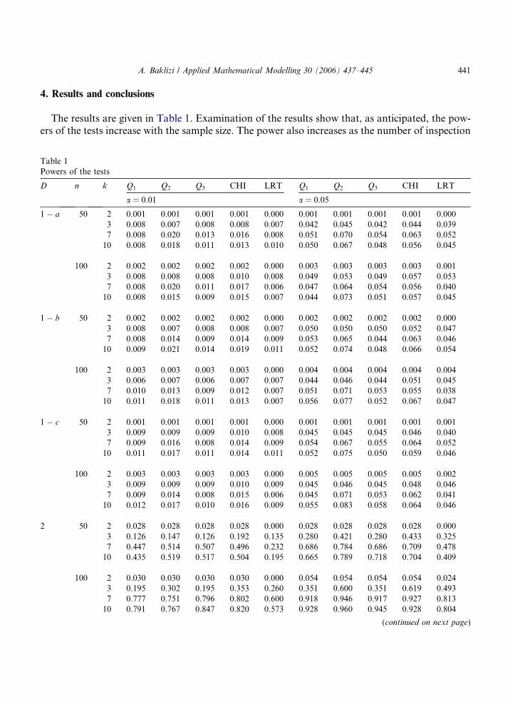
The results are given in Table 1. Examination of the results show that, as anticipated, the pow-ers of the tests increase with the sample size. The power also increases as the number of inspection

Table 1Powers of the tests

D n k Q1 Q2 Q3 CHI LRT Q1 Q2 Q3 CHI LRT

a = 0.01 a = 0.05

1 � a 50 2 0.001 0.001 0.001 0.001 0.000 0.001 0.001 0.001 0.001 0.0003 0.008 0.007 0.008 0.008 0.007 0.042 0.045 0.042 0.044 0.0397 0.008 0.020 0.013 0.016 0.008 0.051 0.070 0.054 0.063 0.05210 0.008 0.018 0.011 0.013 0.010 0.050 0.067 0.048 0.056 0.045

100 2 0.002 0.002 0.002 0.002 0.000 0.003 0.003 0.003 0.003 0.0013 0.008 0.008 0.008 0.010 0.008 0.049 0.053 0.049 0.057 0.0537 0.008 0.020 0.011 0.017 0.006 0.047 0.064 0.054 0.056 0.04010 0.008 0.015 0.009 0.015 0.007 0.044 0.073 0.051 0.057 0.045

1 � b 50 2 0.002 0.002 0.002 0.002 0.000 0.002 0.002 0.002 0.002 0.0003 0.008 0.007 0.008 0.008 0.007 0.050 0.050 0.050 0.052 0.0477 0.008 0.014 0.009 0.014 0.009 0.053 0.065 0.044 0.063 0.04610 0.009 0.021 0.014 0.019 0.011 0.052 0.074 0.048 0.066 0.054

100 2 0.003 0.003 0.003 0.003 0.000 0.004 0.004 0.004 0.004 0.0043 0.006 0.007 0.006 0.007 0.007 0.044 0.046 0.044 0.051 0.0457 0.010 0.013 0.009 0.012 0.007 0.051 0.071 0.053 0.055 0.03810 0.011 0.018 0.011 0.013 0.007 0.056 0.077 0.052 0.067 0.047

1 � c 50 2 0.001 0.001 0.001 0.001 0.000 0.001 0.001 0.001 0.001 0.0013 0.009 0.009 0.009 0.010 0.008 0.045 0.045 0.045 0.046 0.0407 0.009 0.016 0.008 0.014 0.009 0.054 0.067 0.055 0.064 0.05210 0.011 0.017 0.011 0.014 0.011 0.052 0.075 0.050 0.059 0.046

100 2 0.003 0.003 0.003 0.003 0.000 0.005 0.005 0.005 0.005 0.0023 0.009 0.009 0.009 0.010 0.009 0.045 0.046 0.045 0.048 0.0467 0.009 0.014 0.008 0.015 0.006 0.045 0.071 0.053 0.062 0.04110 0.012 0.017 0.010 0.016 0.009 0.055 0.083 0.058 0.064 0.046

2 50 2 0.028 0.028 0.028 0.028 0.000 0.028 0.028 0.028 0.028 0.0003 0.126 0.147 0.126 0.192 0.135 0.280 0.421 0.280 0.433 0.3257 0.447 0.514 0.507 0.496 0.232 0.686 0.784 0.686 0.709 0.47810 0.435 0.519 0.517 0.504 0.195 0.665 0.789 0.718 0.704 0.409

100 2 0.030 0.030 0.030 0.030 0.000 0.054 0.054 0.054 0.054 0.0243 0.195 0.302 0.195 0.353 0.260 0.351 0.600 0.351 0.619 0.4937 0.777 0.751 0.796 0.802 0.600 0.918 0.946 0.917 0.927 0.81310 0.791 0.767 0.847 0.820 0.573 0.928 0.960 0.945 0.928 0.804

(continued on next page)

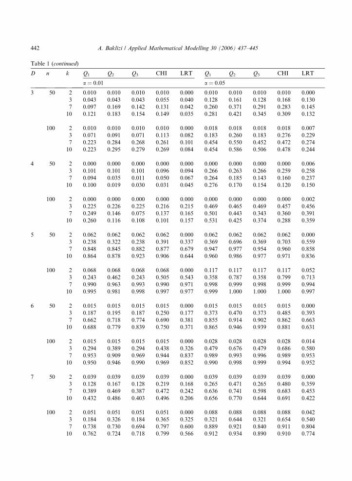
Table 1 (continued)

D n k Q1 Q2 Q3 CHI LRT Q1 Q2 Q3 CHI LRT

a = 0.01 a = 0.05

3 50 2 0.010 0.010 0.010 0.010 0.000 0.010 0.010 0.010 0.010 0.0003 0.043 0.043 0.043 0.055 0.040 0.128 0.161 0.128 0.168 0.1307 0.097 0.169 0.142 0.131 0.042 0.260 0.371 0.291 0.283 0.14510 0.121 0.183 0.154 0.149 0.035 0.281 0.421 0.345 0.309 0.132

100 2 0.010 0.010 0.010 0.010 0.000 0.018 0.018 0.018 0.018 0.0073 0.071 0.091 0.071 0.113 0.082 0.183 0.260 0.183 0.276 0.2297 0.223 0.284 0.268 0.261 0.101 0.454 0.550 0.452 0.472 0.27410 0.223 0.295 0.279 0.269 0.084 0.454 0.586 0.506 0.478 0.244

4 50 2 0.000 0.000 0.000 0.000 0.000 0.000 0.000 0.000 0.000 0.0063 0.101 0.101 0.101 0.096 0.094 0.266 0.263 0.266 0.259 0.2587 0.094 0.035 0.011 0.050 0.067 0.264 0.185 0.143 0.160 0.23710 0.100 0.019 0.030 0.031 0.045 0.276 0.170 0.154 0.120 0.150

100 2 0.000 0.000 0.000 0.000 0.000 0.000 0.000 0.000 0.000 0.0023 0.225 0.226 0.225 0.216 0.215 0.469 0.465 0.469 0.457 0.4567 0.249 0.146 0.075 0.137 0.165 0.501 0.443 0.343 0.360 0.39110 0.260 0.116 0.108 0.101 0.157 0.531 0.425 0.374 0.288 0.359

5 50 2 0.062 0.062 0.062 0.062 0.000 0.062 0.062 0.062 0.062 0.0003 0.238 0.322 0.238 0.391 0.337 0.369 0.696 0.369 0.703 0.5597 0.848 0.845 0.882 0.877 0.679 0.947 0.977 0.954 0.960 0.85810 0.864 0.878 0.923 0.906 0.644 0.960 0.986 0.977 0.971 0.836

100 2 0.068 0.068 0.068 0.068 0.000 0.117 0.117 0.117 0.117 0.0523 0.243 0.462 0.243 0.505 0.543 0.358 0.787 0.358 0.799 0.7137 0.990 0.963 0.993 0.990 0.971 0.998 0.999 0.998 0.999 0.99410 0.995 0.981 0.998 0.997 0.977 0.999 1.000 1.000 1.000 0.997

6 50 2 0.015 0.015 0.015 0.015 0.000 0.015 0.015 0.015 0.015 0.0003 0.187 0.195 0.187 0.250 0.177 0.373 0.470 0.373 0.485 0.3937 0.662 0.718 0.774 0.690 0.381 0.855 0.914 0.902 0.862 0.66310 0.688 0.779 0.839 0.750 0.371 0.865 0.946 0.939 0.881 0.631

100 2 0.015 0.015 0.015 0.015 0.000 0.028 0.028 0.028 0.028 0.0143 0.294 0.389 0.294 0.438 0.326 0.479 0.676 0.479 0.686 0.5807 0.953 0.909 0.969 0.944 0.837 0.989 0.993 0.996 0.989 0.95310 0.950 0.946 0.990 0.969 0.852 0.990 0.998 0.999 0.994 0.952

7 50 2 0.039 0.039 0.039 0.039 0.000 0.039 0.039 0.039 0.039 0.0003 0.128 0.167 0.128 0.219 0.168 0.265 0.471 0.265 0.480 0.3597 0.389 0.469 0.387 0.472 0.242 0.636 0.741 0.598 0.683 0.45310 0.432 0.486 0.403 0.496 0.206 0.656 0.770 0.644 0.691 0.422

100 2 0.051 0.051 0.051 0.051 0.000 0.088 0.088 0.088 0.088 0.0423 0.184 0.326 0.184 0.365 0.325 0.321 0.644 0.321 0.654 0.5407 0.738 0.730 0.694 0.797 0.600 0.889 0.921 0.840 0.911 0.80410 0.762 0.724 0.718 0.799 0.566 0.912 0.934 0.890 0.910 0.774

442 A. Baklizi / Applied Mathematical Modelling 30 (2006) 437–445

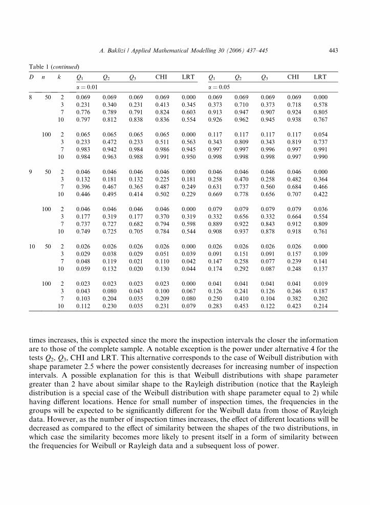
Table 1 (continued)

D n k Q1 Q2 Q3 CHI LRT Q1 Q2 Q3 CHI LRT

a = 0.01 a = 0.05

8 50 2 0.069 0.069 0.069 0.069 0.000 0.069 0.069 0.069 0.069 0.0003 0.231 0.340 0.231 0.413 0.345 0.373 0.710 0.373 0.718 0.5787 0.776 0.789 0.791 0.824 0.603 0.913 0.947 0.907 0.924 0.80510 0.797 0.812 0.838 0.836 0.554 0.926 0.962 0.945 0.938 0.767

100 2 0.065 0.065 0.065 0.065 0.000 0.117 0.117 0.117 0.117 0.0543 0.233 0.472 0.233 0.511 0.563 0.343 0.809 0.343 0.819 0.7377 0.983 0.942 0.984 0.986 0.945 0.997 0.997 0.996 0.997 0.99110 0.984 0.963 0.988 0.991 0.950 0.998 0.998 0.998 0.997 0.990

9 50 2 0.046 0.046 0.046 0.046 0.000 0.046 0.046 0.046 0.046 0.0003 0.132 0.181 0.132 0.225 0.181 0.258 0.470 0.258 0.482 0.3647 0.396 0.467 0.365 0.487 0.249 0.631 0.737 0.560 0.684 0.46610 0.446 0.495 0.414 0.502 0.229 0.669 0.778 0.656 0.707 0.422

100 2 0.046 0.046 0.046 0.046 0.000 0.079 0.079 0.079 0.079 0.0363 0.177 0.319 0.177 0.370 0.319 0.332 0.656 0.332 0.664 0.5547 0.737 0.727 0.682 0.794 0.598 0.889 0.922 0.843 0.912 0.80910 0.749 0.725 0.705 0.784 0.544 0.908 0.937 0.878 0.918 0.761

10 50 2 0.026 0.026 0.026 0.026 0.000 0.026 0.026 0.026 0.026 0.0003 0.029 0.038 0.029 0.051 0.039 0.091 0.151 0.091 0.157 0.1097 0.048 0.119 0.021 0.110 0.042 0.147 0.258 0.077 0.239 0.14110 0.059 0.132 0.020 0.130 0.044 0.174 0.292 0.087 0.248 0.137

100 2 0.023 0.023 0.023 0.023 0.000 0.041 0.041 0.041 0.041 0.0193 0.043 0.080 0.043 0.100 0.067 0.126 0.241 0.126 0.246 0.1877 0.103 0.204 0.035 0.209 0.080 0.250 0.410 0.104 0.382 0.20210 0.112 0.230 0.035 0.231 0.079 0.283 0.453 0.122 0.423 0.214

A. Baklizi / Applied Mathematical Modelling 30 (2006) 437–445 443

times increases, this is expected since the more the inspection intervals the closer the informationare to those of the complete sample. A notable exception is the power under alternative 4 for thetests Q2, Q3, CHI and LRT. This alternative corresponds to the case of Weibull distribution withshape parameter 2.5 where the power consistently decreases for increasing number of inspectionintervals. A possible explanation for this is that Weibull distributions with shape parametergreater than 2 have about similar shape to the Rayleigh distribution (notice that the Rayleighdistribution is a special case of the Weibull distribution with shape parameter equal to 2) whilehaving different locations. Hence for small number of inspection times, the frequencies in thegroups will be expected to be significantly different for the Weibull data from those of Rayleighdata. However, as the number of inspection times increases, the effect of different locations will bedecreased as compared to the effect of similarity between the shapes of the two distributions, inwhich case the similarity becomes more likely to present itself in a form of similarity betweenthe frequencies for Weibull or Rayleigh data and a subsequent loss of power.

444 A. Baklizi / Applied Mathematical Modelling 30 (2006) 437–445

As to the comparison for the five competing tests, it appears that the Q2 test and the chi-squared test have the best performance with the chi-squared test better for smaller significance lev-els or smaller number of inspection intervals, and the Q2 test better otherwise. Overall, the worsttest in terms of power appears to be the LRT.

A general comment concerning the number of inspection times, the powers of the tests are quitelow for k = 2, a much greater power can be achieved by increasing the increasing k by only 1, thatis for k = 3. Greater power could be achieved by increasing k to 7, but afterward the increase inpower is relatively minor.

5. Recommendations and further research

The results obtained from this study encourage the use of either the chi-squared or the Q2 testdepending on the significance level and the number of intervals (inspection times) chosen. Thework in this paper can be extended in various directions. One can consider other models of prac-tical importance in grouped data settings like the Weibull, lognormal, . . . etc. Another possibilityis to study the choice and number of class boundaries (Inspection times) that lead to the highestpower of a given test. Higher order corrections to the likelihood ratio test Bandorff-Nielsen andCox [14] may be developed and investigated to improve the somewhat bad performance it has inthe present study. Another direction is to modify the tests to situations where there is a possibilityof censoring and withdrawal from the experiment. This possibility is currently under consider-ation by the author.

Acknowledgments

The author thanks the editor and the referee for their careful reading and their comments andsuggestions that improved the paper.

References

[1] K. Pearson, On a criterion that a given system of deviations from the probable in the case of a correlated system ofvariables is such that it can be reasonably supposed to have arisen from random sampling, Philos. Mag., 5th series50 (1900) 157–175.

[2] R.B. D�Agostino, M.A. Stephens (Eds.), Goodness-of-fit Techniques, Marcel Dekker, 1986.[3] A.N. Pettitt, M.A. Stephens, The Kolmogrov–Smirnov goodness-of-fit statistic with discrete and grouped data,

Technometrics 19 (1977) 205–210.[4] P. Schmid, On the Kolmogrov and Smirnov limit theorems for discontinuous distribution functions, Ann. Math.

Stat. 29 (1958) 1011–1027.[5] W.J. Conover, A Kolmogrov goodness-of-fit test for discontinuous distributions, J. Am. Stat. Assoc. 67 (1972)

591–596.[6] U.R. Maag, P. Streit, P.A. Drouilly, Goodness-of-fit test for grouped data, J. Am. Stat. Assoc. 68 (1973) 462–465.[7] H. Reidwyl, Goodness of fit, J. Am. Stat. Assoc. 62 (1967) 390–398.[8] C. Damianou, A.W. Kemp, New goodness of fit statistics for discrete and continuous data, Am. J. Math. Manag.

Sci. 10 (1990) 275–307.

A. Baklizi / Applied Mathematical Modelling 30 (2006) 437–445 445

[9] S. Gulati, J. Neus, Goodness of fit statistics for the exponential distribution when the data are grouped, Commun.Stat.: Theor. Meth. 32 (3) (2003) 681–700.

[10] G. Kulldorff, Estimation from Grouped and Partially Grouped Samples, Wiley, 1961.[11] B. Efron, R. Tibshirani, An Introduction to the Bootstrap, Chapman and Hall, 1993.[12] A.C. Davison, D.V. Hinkley, Bootstrap Methods and Their Application, Cambridge University Press, 1997.[13] A. Agresti, Categorical Data Analysis, Wiley, 1990.[14] O. Barndorff-Neilsen, D.R. Cox, Inference and Asymptotics, Chapman and Hall, 1994.