arX

iv:1

112.

5603

v1 [

cond

-mat

.qua

nt-g

as]

23

Dec

201

1

Weak localization with nonlinear bosonic matter waves

Timo Hartmanna, Josef Michla, Cyril Petitjeanb,c, Thomas Wellensd, Juan-Diego Urbinaa,Klaus Richtera, Peter Schlaghecke

aInstitut fur Theoretische Physik, Universitat Regensburg, 93040 Regensburg, GermanybSPSMS-INAC-CEA, 17 Rue des Martyrs, 38054 Grenoble Cedex 9, FrancecLaboratoire de Physique, ENS Lyon, 46, Allee d’Italie, 69007 Lyon, France

dInstitut fur Physik, Albert-Ludwigs-Universitat Freiburg, Hermann-Herder-Str. 3, 79104 Freiburg,

GermanyeDepartement de Physique, Universite de Liege, 4000 Liege, Belgium

Abstract

We investigate the coherent propagation of dilute atomic Bose-Einstein condensatesthrough irregularly shaped billiard geometries that are attached to uniform incoming andoutgoing waveguides. Using the mean-field description based on the nonlinear Gross-Pita-evskii equation, we develop a diagrammatic theory for the self-consistent stationary scatter-ing state of the interacting condensate, which is combined with the semiclassical represen-tation of the single-particle Green function in terms of chaotic classical trajectories withinthe billiard. This analytical approach predicts a universal dephasing of weak localizationin the presence of a small interaction strength between the atoms, which is found to bein good agreement with the numerically computed reflection and transmission probabilitiesof the propagating condensate. The numerical simulation of this quasi-stationary scatter-ing process indicates that this interaction-induced dephasing mechanism may give rise toa signature of weak antilocalization, which we attribute to the influence of non-universalshort-path contributions.

Keywords:

weak localization, coherent backscattering, Bose-Einstein condensates, semiclassicaltheory, nonlinear wave propagation, quantum transport

1. Introduction

Recent technological advances in the manipulation of ultracold atoms on microscopiclength scales have paved the way towards the exploration of scattering and transport phe-nomena with coherent interacting matter waves. Key experiments in this context includethe creation of flexible waveguide geometries with optical dipole beams [1] and on atomchips [2, 3], the coherent propagation of Bose-Einstein condensed atoms in such waveguidesby means of guided atom lasers [4, 5], the realization of optical billiard confinements [6, 7, 8]and microscopic scattering and disorder potentials for cold atoms [9, 10], as well as the detec-tion of individual atoms within a condensate through photoionization on an atom chip [11].Moreover, it was recently demonstrated [12] that artificial gauge potentials, which lead to a

Preprint submitted to Annals of Physics December 26, 2011

breaking of time-reversal invariance in the same way as do magnetic fields for electrons, canbe induced for cold atoms by means of Raman dressing with two laser beams that include afinite orbital angular momentum [13, 14, 15]. Together with the possibility of combining dif-ferent atomic (bosonic and fermionic) species and of manipulating their interaction throughFeshbach resonances, the combination of these tools gives rise to a number of possible scat-tering and transport scenarios that are now ready for experimental investigation.

A particularly prominent quantum transport phenomenon in mesoscopic physics is weaklocalization [16, 17]. This concept refers to an appreciable enhancement of the reflection (or,in the solid-state context, of the electronic resistance) in the presence of a two- or three-dimensional ballistic or disordered scattering region, as compared to the expectation basedon a classical, i.e. incoherent, transport process. This enhancement, which in turn implies areduction of the transmission (or of the electronic conductance) due to current conservation,is in particular caused by “coherent backscattering”, i.e. by the constructive interferencebetween backscattered classical paths and their time-reversed counterparts, which was firstobserved in experiments on the scattering of laser light from disordered media [18, 19]. Inthe solid-state context, weak localization is most conveniently detected by measuring theelectronic conductance in dependence of a weak magnetic field that is oriented perpendicularto the scattering region, such that it causes a dephasing between backscattered paths andtheir time-reversed counterparts. A characteristic peak structure at zero magnetic field isthen tyipcally observed [20, 21].

From the electronic point of view, the presence of interaction between the particles thatparticipate at this scattering process is generally expected to give rise to an additionaldephasing mechanism of this subtle interference phenomenon [22, 23, 24]. In the contextof ultracold bosonic atoms, this expectation is partly confirmed by previous theoreticalstudies on the coherent propagation of an interacting Bose-Einstein condensate througha two-dimensional disorder potential [25], which employed numerical simulations as wellas diagrammatic representations based on the mean-field description of the condensate interms of the nonlinear Gross-Pitaevskii equation. This study did indeed reveal a reduction ofthe height of the coherent backscattering peak with increasing effective interaction strengthbetween the atoms. It also predicted, however, that this coherent backscattering peak mightturn into a dip at finite (but still rather small) interaction strengths [25]. This scenario isreminiscent of weak antilocalization due to spin-orbit interaction, which was observed inmesoscopic magnetotransport [26].

In order to gain a new perspective on this novel phenomenon, we investigate, in thiswork, the coherent propagation of Bose-Einstein condensates through ballistic scatteringgeometries that exhibit chaotic classical dynamics. Such propagation processes could beexperimentally realized by guided atom lasers in which the optical waveguides are locally“deformed” by means of additional optical potentials (e.g. by focusing another red-detunedlaser onto this waveguide). Alternatively, atom chips [2, 3] or atom-optical billiards [6, 7, 8]could be used in order to engineer chaotic scattering geometries for ultracold atoms. Fromthe theoretical point of view, the wave transport through such scattering geometries can bedescribed using the semiclassical representation of the Green function in terms of classicaltrajectories. The constructive intereference of reflected trajectories with their time-reversed

2

counterparts gives then rise to coherent backscattering [27], while a complete understandingof weak localization, in particular the corresponding reduction of the transmitted current,requires additional, classically correlated trajectory pairs [28, 29].

In order to account for the presence of atom-atom interaction on the mean-field levelof the nonlinear Gross-Pitaevskii equation, we combine, in this paper, the semiclassical ap-proach with the framework of nonlinear diagrammatic theory developed in Refs. [30, 31, 32].For the sake of simplicity, we shall, as is described in Section 2, restrict ourselves to idealchaotic billiard dynamics consisting of free motion that is confined by hard-wall boundaries.Since such billiard geometries give rise to uniform average densities within the scatteringregion, we can, as demonstrated in Sections 3 and 4, derive explicit analytical expressions forthe retro-reflection and transmission probabilities as a function of the effective interactionstrength. As shown in Section 5, these expressions agree very well with the numericallycomputed retro-reflection and transmission probabilities for two exemplary billiard geome-tries as far as the deviation from the case of noninteracting (single-particle) transport isconcerned. On the absolute scale, however, the height of the weak localization peak is re-duced in this noninteracting case by the presence of short-path contributions, in particularby self-retracing trajectories, which, as shown in Section 5, consequently turn this peak intoa finite dip in the presence of a small interaction strength. We shall therefore argue in Sec-tion 6 that such short-path contributions are at the origin of this weak antilocalization-likephenomenon.

2. Setup of the nonlinear scattering process

We consider the quasistationary transport of coherent bosonic matter waves through two-dimensional waveguide structures that are perturbed by the presence of a wide quantum-dot-like scattering potential. Such propagating matter waves can be generated by means ofa guided atom laser [4, 5] where ultracold atoms are coherently outcoupled from a trappingpotential that contains a Bose-Einstein condensate. The control of the outcoupling process,which, e.g., can be achieved by applying a radiofrequency field that flips the spin of theatoms in the (magnetic) trap [4], permits one, in principle, to generate an energeticallywell-defined beam of atoms that propagate along the (horizontally oriented) waveguide inits transverse ground mode [33]. This waveguide, as well as the quantum-dot-like scatteringpotential, can be engineered by means of focused red-detuned laser beams which providean attractive effective potential for the atoms that is proportional to their intensity. Therestriction to two spatial dimensions can, furthermore, be realized by applying, in addition,a tight one-dimensional optical lattice perpendicular to the waveguide (i.e. oriented alongthe vertical direction).

The central object of study in this work is the phenomenon of weak localization. Inthe context of electronic mesoscopic physics, this quantum interference phenomenon can bedetected by measuring the electronic conductance, which is directly related to the quantumtransmission through the Landauer-Buttiker theory [34, 35, 36], as a function of the strengthof an externally applied magnetic field which breaks time-reversal invariance within the scat-tering region. Such a time-reversal breaking mechanism can also be induced for cold atoms

3

xL

W~

W

a

xL

W~

b

W

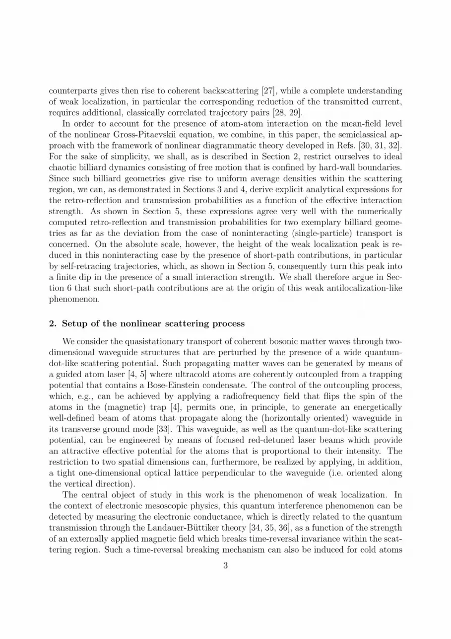
Figure 1: Shapes of the billiards a and b under consideration, plotted together with the density of a stationaryscattering state. We indicate, in addition, the widths W and W of the incident and the transmittedwaveguides, respectively, as well as the horizontal position xL at which the incident and reflected parts ofthe scattering wavefunction are decomposed in transverse eigenmodes of the waveguide. The semiclassicalaverage that is undertaken in order to obtain the mean retro-reflection probability involves an average ofthe retro-reflection probability within a finite window of chemical potentials µ for different incident channelsand different locations of the circular and the lower semicircular obstacle in the case of billiards a and b,respectively.

[12, 13, 14, 15], e.g., by coherently coupling two intra-atomic levels via a STIRAP process,using two laser beams of which one involves a nonvanishing orbital angular momentum [13].This gives rise to an effective vector potential in the kinetic term of the Schrodinger equation,which is assumed such that it generates an effective “magnetic field” that is homogeneouswithin the scattering region and vanishes within the attached waveguides.

The main purpose of this study is to investigate how the scenario of weak localizationis affected by the presence of a weak atom-atom interaction within the matter-wave beam.In lowest order in the interaction strength, the presence of such an atom-atom interactionis accounted for by a nonlinear contribution to the effective potential in the Schrodingerequation describing the motion of the atoms, which is proportional to the local density ofatoms and which gives rise to the celebrated Gross-Pitaevskii equation [37]. The strengthof this nonlinear contribution can be controlled by the scale of the confinement in thetransverse (vertical) spatial direction. We shall make, in the following, the simplifyingassumption that this nonlinearity is present only within the scattering region and vanisheswithin the waveguides. We furthermore assume that the waveguides are perfectly uniform,and that the two-dimensional scattering geometry can be described by perfect “billiard”potentials which combine a vanishing potential background within the waveguides and thescattering region with infinitely high hard walls along their boundaries. These assumptionsconsiderably simplify the analytical and numerical treatment of the problem, and allow forthe identification of well-defined asymptotic scattering states within the waveguides. Twosuch billiard configurations are shown in Fig. 1.

The dynamics of this matter-wave scattering process is then well modelled by an inho-

4

mogeneous two-dimensional Gross-Pitaevskii equation [38]

i~∂

∂tΨ(r, t) =

[− 1

2m

(~

i∇−A(r)

)2

+ V (r) + g~2

2m|Ψ(r, t)|2

]Ψ(r, t) + S(r, t) (1)

with r ≡ (x, y). Here m is the mass of the atoms and V (r) represents the confinementpotential that defines the waveguides and the scattering region. The effective vector potentialA(r) vanishes within the waveguides. Within the scattering billiard we choose it as

A(r) ≡ 1

2Bez × (r− r0) =

1

2B[(x− x0)ey − (y − y0)ex] (2)

where r0 ≡ (x0, y0) represents an arbitrarily chosen reference point and ex, ey, ez are theunit vectors in our spatial coordinate system. In the presence of an harmonic transverse(vertical) confinement with oscillation frequency ω⊥ ≡ ω⊥(r), the effective two-dimensionalinteraction strength is given by g(r) = 4

√2πas/a⊥(r) with a⊥(r) ≡

√~/[mω⊥(r)] where as

denotes the s-wave scattering length of the atoms. As stated above, we assume that g isconstant within the billiard and vanishes in the waveguides.

The source amplitude S(r, t) describes the coherent injection of atoms from the Bose-Einstein condensate within the reservoir trap. Assuming that only one transverse eigenmodein the waveguide is populated, we may write S as

S(r, t) = S0χi(y)δ(x− xL)exp

(− i

~µt

)(3)

where χi(y) denotes the normalized wavefunction associated with the transverse eigenmodewith the excitation index i, characterized by the energy Ei, into which the source injects theatoms from the condensate (typically one would attempt to achieve coherent injection intothe transverse ground mode, with i = 1, in an atom-laser experiment [4]). xL represents anarbitrary longitudinal coordinate within the waveguide (which, without loss of generality,is assumed to be oriented along the x axis) and µ is the chemical potential with which theatoms are injected into the waveguide. Making the ansatz

Ψ(r, t) ≡ ψ(r, t)exp

(− i

~µt

)(4)

we obtain

i~∂

∂tψ(r, t) = (H − µ)ψ(r, t) + g

~2

2m|ψ(r, t)|2ψ(r, t) + S0χi(y)δ(x− xL) (5)

with the single-particle Hamiltonian

H =1

2m

[~

i∇−A(r)

]2+ V (r) . (6)

5

The time evolution of the scattering wavefunction can be considered to take place inthe presence of an adiabatically slow increase of the source amplitude S0 from zero to agiven maximal value. In the absence of interaction, this process would necessarily lead to astationary scattering state, whose decomposition into the transverse eigenmodes within thewaveguides allows one to determine the associated channel-resolved reflection and transmis-sion amplitudes. In the special case of a perfectly uniform waveguide without any scatteringpotential and in the absence of the vector potential A, this stationary state is given by

ψ(x, y) = −i mS0

~pli(µ)χi(y) exp

[− i

~pli(µ) |x− xL|

](7)

where pli(µ) ≡√2mµ−Ei denotes the longitudinal component of the momentum associated

with the transverse mode χi. Such a stationary scattering state is, in general, not obtainedin the presence of interaction. Indeed, a finite nonlinearity strength g may, in combinationwith a weak scattering potential, lead to a permanently time-dependent, turbulent-like flowacross the scattering region [39, 40, 41, 25, 38], which in dimensionally restricted waveguidegeometries should correspond to a loss of coherence on a microscopic level of the many-bodyscattering problem [38].

In the following, we shall restrict ourselves to rather small nonlinearities for which westill obtain, in most cases, stable quasistationary scattering states within the billiard underconsideration [42]. In the subsequent two sections, we shall develop a semiclassical theoryfor the self-consistent scattering state that is obtained as a solution of Eq. (5). Section 3focuses on contributions related to coherent backscattering, while loop corrections in next-to leading order in the inverse number of energetically accessible channels are taken intoaccount in section 4.

3. Semiclassical theory of nonlinear coherent backscattering

3.1. Coherent backscattering in the linear case

The key ingredient of a semiclassical description of this nonlinear scattering process isthe representation of the retarded quantum Green function

G0(r, r′, E) ≡ 〈r|(E −H0 + i0)−1|r′〉 (8)

in terms of all classical (single-particle) trajectories (pγ,qγ)(t) within the billiard, indexedby γ, that propagate from the initial point r′ to the final point r at total energy E. Here,we deliberately exclude the vector potential A(r), i.e. the underlying Hamiltonian is givenby

H0 =p2

2m+ V (r) (9)

where p ≡ −i~∇ represents the quantum momentum operator. The semiclassical repre-sentation of the Green function can be derived from the Fourier transform of the quantum

6

propagator in Feynman’s path integral representation, which is evaluated in the formal limit~ → 0 using the method of stationary phase. It reads [43]

G0(r, r′, E) =

∑

γ

Aγ(r, r′, E)exp

[i

~Sγ(r, r

′, E)− iπ

2µγ

]. (10)

Here,

Sγ(r, r′, E) =

∫ Tγ

0

pγ(t) · qγ(t)dt (11)

is the classical action integral along the trajectory γ (Tγ denotes the total propagation timefrom r′ to r), µγ represents the integer Maslov index that counts the number of conjugatepoints along the trajectory (which, in a billiard, also involves twice the number of bouncingsat the walls, in addition to the number of conjugate points inside the billiard), and

Aγ(r, r′, E) =

2π√2πi~

3

√| detD2Sγ(r, r′, E)| (12)

is an amplitude that smoothly depends on r and r′, with

| detD2Sγ(r, r′, E)| =

∣∣∣∣det∂(p′, r′, T )

∂(r, r′, E)

∣∣∣∣ . (13)

the Jacobian of the transformation from the initial phase space variables (p′, r′) and thepropagation time T to the final and initial positions (r, r′) and the energy E.

The presence of a weak effective magnetic field is now incorporated in a perturbativemanner using the eikonal approximation. As shown in Appendix Appendix B, this yieldsthe well-known modification of the Green function

G(r, r′, E) =∑

γ

Aγ(r, r′, E) exp

i

~[Sγ(r, r

′, E)− φγ(r, r′, E)]− i

π

2µγ

(14)

with φγ(r, r′, E) = −ϕγ(r, r

′, E)− ϕγ(r, r′, E) and

ϕγ(r, r′, E) ≡ 1

m

∫ Tγ

0

pγ(t) ·A[qγ(t)]dt , (15)

ϕ(d)γ (r, r′, E) ≡ − 1

2m

∫ Tγ

0

A2[qγ(t)]dt (16)

where the integration is peformed along the unperturbed trajectory qγ(t). While the latter

(diamagnetic) contribution ϕ(d)γ gives only rise to a spatial modulation of the effective po-

tential background within the billiard, the former (paramagnetic) contribution ϕγ explicitlybreaks the time-reversal symmetry of the system and plays a crucial role for the intensity ofcoherent backscattering.

7

This expression for the Green function can be directly used in order to construct thescattering state ψ(r) that arises as a stationary solution of Eq. (5). We obtain

ψ(r) = S0

∫G[r, (xL, y

′), µ]χi(y′)dy′ (17)

where χi represents the energetically lowest transverse eigenmode within the waveguide.Assuming billiard-like waveguides with a vanishing potential background and infinitely highhard walls along their boundaries, the nth normalized transverse eigenmode (n > 0) is givenby

χn(y) =

√2

Wsin(pny

~

)=

1

2i

√2

W

[exp

(i

~pny

)− exp

(− i

~pny

)]for 0 ≤ y ≤W (18)

and χn(y) = 0 otherwise. pn ≡ nπ~/W is the quantized transverse momentum and Wrepresents the width of the waveguide. We can therefore write

ψ(r) =S0

i

√π~

W

G [r, (xL, pi), µ]−G [r, (xL,−pi), µ]

(19)

where

G[r, (x′, p′y), E] ≡1√2π~

∫ W

0

G[r, (x′, y′), E]exp

(i

~p′yy

′

)dy′ (20)

denotes a partial Fourier transform of G[r, (x′, y′), E].Inserting the semiclassical expression (14) for the Green function G, this partial Fourier

transform can again be evaluated using the stationary phase approximation. The stationaryphase condition yields (pi

γ)y[r, (x′, y′), E] = p′y, i.e. p

′y should be the y-component of the

initial momentum of the trajectory. The integration over y′ yields the prefactor√

2πi~/αwith

α ≡ ∂2

∂y′2Sγ [r, (x

′, y′), E] = −∂[r, (x′, p′y), E]

∂[r, (x′, y′), E]. (21)

Combining it with the prefactor√

| detD2Sγ | according to the expression (13) and with theother prefactors that are contained within the amplitude Aγ , we finally obtain

G(r, z′, E) =∑

γ

Aγ(r, z′, E) exp

i

~

[Sγ(r, z

′, E)− φγ(r, z′, E)

]−iπ

2µγ

(22)

with

Aγ(r, z′, E) =

2π√i

√2πi~

3

√∣∣∣∣det∂[p′, (x′, y′), T ]

∂[r, (x′, p′y), E]

∣∣∣∣ , (23)

µγ = µγ +

1 : ∂2

∂y′2Sγ(r, r

′, E) < 0

0 : otherwise, (24)

Sγ(r, z′, E) = Sγ

r,[x′, y′γ(r, z

′, E)], E+ p′yy

′γ(r, z

′, E) , (25)

8

and φγ(r, z′, E) defined according to Eq. (B.9), where the initial phase-space point of the

trajectories γ is given by the combination z′ ≡ (x′, p′y) and y′γ(r, z

′, E) denotes the resultinginitial y coordinate.

Channel-resolved reflection and transmission amplitudes can now be computed by pro-jecting ψ onto the transverse eigenmodes of the waveguides. This involves again a partialFourier transform of the Green function, this time in the final coordinate. In particular, thereflection amplitude into channel n is obtained from

ψn ≡∫ W

0

χ∗n(y)ψ(xL, y)dy (26)

= S0π~

W

G[(xL, pn), (xL, pi), µ]− G[(xL, pn), (xL,−pi), µ]

−G[(xL,−pn), (xL, pi), µ] + G[(xL,−pn), (xL,−pi), µ]

≡ S0π~

W

[G(z−n , z

+1 , µ)− G(z+n , z

+1 , µ)− G(z−n , z

−1 , µ) + G(z+n , z

−1 , µ)

](27)

with

G[(x, py), r′, E] ≡ 1√

2π~

∫ W

0

G[(x, y), r′, E]exp

(− i

~pyy

)dy , (28)

G[(x, py), z′, E] ≡ 1√

2π~

∫ W

0

G[(x, y), z′, E]exp

(− i

~pyy

)dy (29)

where we define

z±n ≡

(xL,±pn) for incoming trajectories (with p′x > 0)(xL,∓pn) for outgoing trajectories (with px < 0)

. (30)

Similarly as for G, the semiclassical evaluation of this Fourier transform using Eq. (22) yields[27, 44, 45]

G(z, z′, E) =∑

γ

Aγ(z, z′, E) exp

i

~

[Sγ(z, z

′, E)− φγ(z, z′, E)

]−iπ

2µγ

(31)

with

Aγ(z, z′, E) =

2πi√2πi~

3

√∣∣∣∣det∂[(p′x, p

′y), (x

′, y′), T ]

∂[(x, py), (x′, p′y), E]

∣∣∣∣ , (32)

µγ = µγ +

1 : ∂2

∂y2Sγ(r, z

′, E) < 0

0 : otherwise, (33)

Sγ(z, z′, E) = Sγ [x, yγ(z, z′, E)] , z′, E − pyyγ(z, z

′, E) , (34)

and φγ(z, z′, E) defined according to Eq. (B.9), where the final phase-space point of the

trajectories γ is given by the combination z ≡ (x, py) (and yγ is the final y coordinate).

9

From Eq. (31) it becomes obvious that subtle interferences between different classicaltrajectories may give rise to channel-resolved reflection and transmission probabilities thatstrongly fluctuate under variation of the incident chemical potential µ ≡ E. Those fluc-tuations generally cancel, however, when performing an average within a finite window ofchemical potentials. Specifically, the calculation of |ψn|2 involves sums over pairs of tra-jectories γ and γ′, whose contributions contain phase factors that depend on the difference

Sγ− Sγ′ of the associated action integrals. These differences strongly vary with the chemicalpotential µ unless the two trajectories γ and γ′ are somehow correlated.

An obvious correlation arises if the two trajectories happen to be identical, in which casethe phase factor is unity. In the framework of the diagonal approximation, we only take intoaccount this specific case, i.e., we approximate the double sum

∑γ,γ′ by a single sum

∑γ

where γ′ is taken to be identical to γ. The energy average 〈|ψn|2〉 of |ψn|2 is then given by

〈|ψn|2〉 ≃ 〈|ψn|2〉d (35)

=

∣∣∣∣S0π~

W

∣∣∣∣2 [⟨∣∣∣G(z+n , z+1 , µ)

∣∣∣2⟩

d

+

⟨∣∣∣G(z+n , z−1 , µ)∣∣∣2⟩

d

+

⟨∣∣∣G(z−n , z+1 , µ)∣∣∣2⟩

d

+

⟨∣∣∣G(z−n , z−1 , µ)∣∣∣2⟩

d

](36)

with

⟨∣∣∣G(z, z′, E)∣∣∣2⟩

d

=∑

γ

⟨∣∣∣Aγ(z, z′, E)

∣∣∣2⟩.

As shown in Appendix Appendix C, this sum is evaluated using the generalized Hannay-Ozorio de Almeida sum rule [46, 47]. Defining by τD the “dwell time” of the system, i.e. themean evolution time that a classical trajectory spends within the billiard before escapingto one of the waveguides, and introducing the “Heisenberg time” as τH ≡ mΩ/~ where Ωdenotes the area of the billiard, we obtain [see Eq. (C.15)]

⟨∣∣∣G(z, z′, E)∣∣∣2⟩

d

=

(mW

2π~2

)2τDτH

1√2mE − p2y

1√2mE − p′2y

. (37)

Inserting this expression into Eq. (36) and defining

pln(E) ≡√

2mE − p2n =√

2mE − (nπ~/W )2 (38)

as the longitudinal component of the momentum that is associated with the transverse modeχn finally yields

〈|ψn|2〉d =

∣∣∣∣mS0

~

∣∣∣∣2τDτH

1

pln(µ)pli(µ)

. (39)

This expression can be used in order to determine the steady current jn of atoms that arereflected into channel n, according to

jn =pln(µ)

m〈|ψn|2〉 . (40)

10

Dividing it by the incident current which is derived from Eq. (7) as

ji =m|S0|2~2pli(µ)

, (41)

we obtain the reflection probability into channel n as

rni ≡ jn/ji = τD/τH . (42)

The same reasoning can be applied to the outgoing waveguide on the other, transmittedside of the billiard. Again we obtain tni = τD/τH as the probability for transmission intothe transverse channel n of the outgoing waveguide, even if its witdh W is different fromthe width W of the incoming guide. The total reflection and transmission probabilities Rand T are then simply related to the numbers of open channels Nc and Nc in the incomingand outgoing waveguide according to R = NcτD/τH and T = NcτD/τH , where we evaluateNc = 2W/λdB and Nc = 2W/λdB in the semiclassical limit, with λdB ≡ 2π~/

√2mµ the de

Broglie wavelength of the atoms. We can furthermore use the general expression [27, 28]

τD =πΩ

(W + W )v(43)

for the mean survival time of a classical particle propagating with velocity v in a chaoticbilliard with area Ω that contains two openings of width W and W , which yields

τDτH

=λdB/2

W + W=

1

Nc + Nc

. (44)

We then arrive at the intuitive results R = W/(W + W ) and T = W/(W + W ), i.e. thetotal reflection and transmission probabilities are simply given by the relative widths of thecorresponding waveguides.

The diagonal approximation therefore yields predictions for reflection and transmissionthat are expected for incoherent, classical particles in a chaotic cavity. It represents inleading order in the inverse total channel number (Nc + Nc)

−1 the contributions for allchannels on the transmitted side, and for all reflected channels except for the channel n = iin which the matter-wave beam is injected into the billiard. In this incident channel, thereis another, equally important possibility to pair the trajectories γ and γ′ in the doublesums that are involved in the calculation of |ψi|2: γ′ can be chosen to be the time-reversed

counterpart of γ, the existence of which is guaranteed by the time-reversal symmetry of H0.Consequently, Eq. (35) has to be corrected for the special case n = i according to

〈|ψi|2〉 ≃ 〈|ψi|2〉d + 〈|ψi|2〉c (45)

where the “crossed” or “Cooperon”-type contribution

〈|ψi|2〉c =

∣∣∣∣S0π~

W

∣∣∣∣2 [⟨∣∣∣G(z+i , z+i , µ)

∣∣∣2⟩

c

+

⟨∣∣∣G(z−i , z−i , µ)∣∣∣2⟩

c

+⟨G

∗

(z+i , z−i , µ) G(z

−i , z

+i , µ)

⟩

c+⟨G

∗

(z−i , z+i , µ) G(z

+i , z

−i , µ)

⟩

c

](46)

11

contains all those combinations of trajectories for which γ′ is the time-reversed counterpart of

γ. Obviously, the action integrals Sγ and Maslov indices µγ are identical for the trajectoriesγ and their time-reversed counterparts. This is not the case, however, for the modification

φγ of the action integral that is induced by the vector potential, whose paramagnetic part

ϕγ [Eq. (15)] changes sign when integrating along the trajectory γ in the opposite direction.We therefore obtain

⟨G

∗

(z′, z, E) G(z, z′, E)⟩c=∑

γ

⟨∣∣∣Aγ(z, z′, E)

∣∣∣2

exp

[2i

~ϕγ(z, z

′, E)

]⟩. (47)

To provide some physical insight into the role of this additional phase factor, we use therepresentation (2) of the vector potential within the billiard. Using pγ(t) = mqγ(t) alongtrajectories γ generated by H0, the paramagnetic contribution to the effective action integralreads then

ϕγ(z, z′, E) =

B

2ez ·

∫ Tγ

0

[qγ(t)− r0]× qγ(t) dt (48)

where r0 is an arbitrarily chosen reference point. Within the billiard, the trajectories(pγ,qγ)(t) can be decomposed into segments of straight lines that connect subsequent re-

flection points at the billiard boundary. Denoting those reflection points by q(1)γ , . . . ,q

(N−1)γ

and defining q(0)γ ≡ r′ and q

(N)γ ≡ r, the initial and final points of the trajectory, we rewrite

Eq. (48) as

ϕγ(z, z′, E) = B

N∑

j=1

aj≡BA (49)

where

aj =1

2ez ·

[(q(j−1)

γ − r0)× (q(j)γ − r0)

](50)

is the directed area of the triangle spanned by the reflection points q(j−1)γ and q

(j)γ as well as by

the reference point r0. Quite obviously, ϕγ is independent of the particular choice of r0, or ofany other gauge transformation A 7→ A+∇χ that vanishes within the waveguide, providedthe initial and final points r′ and r of the trajectory γ are identical or, less restrictively, lieboth within the same, incident waveguide where the vector potential vanishes (in which casea straight-line integration

∫A · dq from r′ to r would formally close the trajectory without

adding any further contribution to ϕγ).The central limit theorem is now applied in order to obtain the probability distribution

P (Tγ,A) for accumulating the area A after the propagation time Tγ [27, 28, 44, 45]. Wehave

P (Tγ,A) =1√

πηΩ3/2vTγexp

(− A2

ηΩ3/2vTγ

)(51)

where Ω is the area of the billiard, v is the velocity of the particle, and η is a dimensionlessscaling parameter that characterizes the geometry of the system and that can be numer-ically computed from the classical dynamics within the billiard as described in Appendix

12

Appendix D. This distribution is now used to obtain an average value of the magnetic phasefactor according to

⟨exp

[2i

~ϕγ(z, z

′, E)

]⟩=

∫ +∞

−∞

P (Tγ,A)exp

(2i

~BA

)dA = exp

(−TγτB

)(52)

with

τB ≡ ~2

ηΩ3/2vB2(53)

the characteristic time scale for magnetic dephasing.With this information, we can now follow the derivation of the Hannay-Ozorio de Almeida

sum rule, as explicited in Appendix Appendix C, in order to evaluate the expression (47),with the only complication that each contribution in the sum over trajectories needs to beweighted by the “dephasing” factor exp(−Tγ/τB). This yields⟨G

∗

(z′, z, E) G(z, z′, E)⟩

c=

(mW

2π~2

)2(τHτD

+τHτB

)−11√

2mE − p2y

1√2mE − p′2y

. (54)

Hence, we obtain

〈|ψi|2〉c =∣∣∣∣mS0

~pli(µ)

∣∣∣∣2(

τHτD

+τHτB

)−1

(55)

in very close analogy with Eq. (39), which altogether yields

〈|ψi|2〉 ≃ 〈|ψi|2〉d + 〈|ψi|2〉c =∣∣∣∣mS0

~pli(µ)

∣∣∣∣2(

1 +1

1 + τD/τB

)τDτH

. (56)

This gives rise to an enhanced probability for retro-reflection into the incident channel n = i,namely

rii =

(1 +

1

1 + τD/τB

)τDτH

=

(1 +

1

1 +B2/B20

)τDτH

(57)

with

B0 ≡~√

ηvτDΩ3/2, (58)

as compared to reflection into different channels described by Eq. (42), which is the char-acteristic signature of coherent backscattering. Note that, due to conservation of the totalflux, increased retro-reflection for n = i implies decreased reflection or transmission intoother channels n 6= i. This will be subject of Section 4 below.

The above prediction (57) is expected to be valid for chaotic cavities in the semiclassicallimit of small ~ (i.e. of a small de Broglie wavelength as compared to the size of the scatteringregion) and in the limit of small widths of the leads. Leads of finite widths, as the ones thatare considered in the scattering geometries shown in Fig. 1, will give rise to non-universalcorrections to Eq. (57) that are related to short reflected or transmitted paths. In particular,

13

the presence of self-retracing trajectories, which are identical to their time-reversed coun-terparts, affects the probability for retro-reflection due to coherent backscattering, as thosetrajectories are evidently doubly counted in the addition of ladder and crossed contributions.Hence, the enhancement of this retro-reflection probability with respect to the incoherentladder background (42) will, in practice, be reduced as compared to Eq. (57), due to thepresence of short and therefore semiclassically relevant self-retracing trajectories.

3.2. Diagrammatic representation of nonlinear scattering states

We now consider the presence of a weak interaction strength g > 0 in the Gross-Pitaevskiiequation (5). As a consequence, the scattering process becomes nonlinear and the final(stationary or time-dependent) scattering state may depend on the “history” of the process,i.e. on the initial matter-wave population within the scattering region as well as on thespecific ramping process of the source amplitude. We shall assume that the scatteringregion is initially empty (i.e., ψ(r, t) = 0 for t → −∞) and that the source amplitude S0 isadiabatically ramped from zero to a given maximal value S0, on a time scale that is muchlarger than any other relevant time scale of the scattering system. This adiabatic rampingis formally expressed as S0(t) = S0f(t/tR) where f(τ) is a real dimensionless function thatmonotonously increases from 0 (for t→ −∞) to 1 (for t→ ∞) and tR → ∞ is a very largeramping time scale. Redefining ψ(r, t) ≡ f(t/tR)ψ(r, t) and neglecting terms of the order of1/tR, we obtain from Eq. (5)

i~∂

∂tψ(r, t) = (H − µ)ψ(r, t) + S(r, t) (59)

as effective Gross-Pitaevskii equation for ψ, with

S(r, t) ≡ S0χi(y)δ(x− xL) + g(t)~2

2m|ψ(r, t)|2ψ(r, t) (60)

and g(t) ≡ f 2(t/tR)g. For weak enough nonlinearities g and long enough ramping timescales tR, Eq. (59) can be considered as describing an effectively linear scattering problemthe source term of which is gradually adapted according to Eq. (60). We can thereforeexpress the time-dependent scattering wavefunction as

ψ(r, t) =

∫d2r′G(r, r′, µ)S(r′, t) (61)

where G ≡ (µ−H+i0)−1 is the Green function of the linear scattering problem [see Eq. (14)].In the limit of long evolution times t→ ∞, we thereby obtain

ψ(r) = S0

∫G[r, (xL, y

′), µ]χi(y′)dy′ +

∫d2r′G(r, r′, µ)g

~2

2m|ψ(r′)|2ψ(r′) (62)

as self-consistent equation for the scattering wavefunction, which generalizes the expression(17) obtained for the linear case.

14

In rather close analogy with the numerical procedure that is employed for computing astationary scattering state, we can construct a self-consistent solution of Eq. (62) by startingwith the expression (17) for the linear case and by iteratively inserting the subsequentexpressions obtained for ψ(r) on the right-hand side of Eq. (62). This naturally leads to apower series in the nonlinearity,

ψ(r) = ψ(0)(r) +∞∑

n=1

gnδψ(n)(r) , (63)

where ψ(0)(r) represents the solution of Eq. (17), i.e. the scattering state of the noninteractingsystem.

It is instructive to evaluate the semiclassical representation of the first-order correctionto the linear scattering wavefunction ψ(0), given by

δψ(1)(r) =~2

2m

∫d2r′G(r, r′, µ)|ψ(0)(r′)|2ψ(0)(r′) . (64)

Using the expression (19) for the scattering state of the noninteracting system, we obtain

δψ(1)(r) =~2

2m

S0

i

√π~

W|S0|2

π~

W

∑

ν1,ν2,ν3=±1

ν1ν2ν3

×∫d2r′G(r, r′, µ)G(r′, zν1i , µ)G

∗(r′, zν2i , µ)G(r

′, zν3i , µ) (65)

with z±1i ≡ z±i as defined in Eq. (30). Inserting the semiclassical expansion for the Green

function, given by Eqs. (14) and (22), yields

δψ(1)(r) =~2

2m

S0

i

√π~

W|S0|2

π~

W

∑

ν1,ν2,ν3=±1

ν1ν2ν3

×∫d2r′

∑

γ0

∑

γ1,γ2,γ3

Aγ0(r, r′, µ)Aγ1(r

′, zν1i , µ)A∗

γ2(r′, zν2i , µ)Aγ3(r

′, zν3i , µ)

× exp

i

~

[Sγ0(r, r

′, µ) + Sγ1(r′, zν1i , µ)− Sγ2(r

′, zν2i , µ) + Sγ3(r′, zν3i , µ)

]

× exp

− i

~

[φγ0(r, r

′, µ) + φγ1(r′, zν1i , µ)− φγ2(r

′, zν2i , µ) + φγ3(r′, zν3i , µ)

]

× exp

[−iπ

2

(µγ0 + µγ1 − µγ2 + µγ3

)](66)

where the indices γ0 and γℓ (ℓ = 1, 2, 3) represent trajectories that connect r′ and r as wellas zνℓi and r′, respectively.

Neglecting, as done in Section 3, the modification of the trajectories γ0 and γ1/2/3 due tothe presence of the weak magnetic field, a stationary-phase evaluation of the spatial integralin Eq. (66) yields the condition

piγ0(r, r

′, µ) + pfγ2(r

′, zν2i , µ) = pfγ1(r

′, zν1i , µ) + pfγ3(r

′, zν3i , µ) . (67)

15

Noting that all involved momenta are evaluated at the same spatial point r′, this conditionis satisfied if and only if

piγ0(r, r′, µ) = pf

γ1(r′, zν1i , µ) and pf

γ2(r′, zν2i , µ) = pf

γ3(r′, zν3i , µ) (68)

orpiγ0(r, r′, µ) = pf

γ3(r′, zν3i , µ) and pf

γ2(r′, zν2i , µ) = pf

γ1(r′, zν1i , µ) (69)

orpiγ0(r, r′, µ) = −pf

γ2(r′, zν2i , µ) and pf

γ1(r′, zν1i , µ) = −pf

γ3(r′, zν3i , µ) (70)

holds true. The cases (68) and (69) are essentially equivalent and imply , in case (68) [or incase (69)], that the trajectories γ2 and γ3 (or γ2 and γ1) are identical and that γ0 representsthe direct continuation of the trajectory γ1 (or γ3) from r′ to r. This latter conditiondetermines the stationary points of r′, which have to lie along the trajectories from zν1i (orzν3i ) to r.

Case (70) is more involved. It implies, on the one hand, that the time-reversed counter-part of trajectory γ3 represent the direct continuation of trajectory γ1 (using the fact thatthe scattering system under consideration is, in the absence of the magnetic field, invariantwith respect to time reversal), which determines the stationary points of r′ along reflectedtrajectories from zν1i to zν3i . On the other hand, γ0 represents a part of the time-reversedcounterpart of trajectory γ2, which necessarily implies that the point of observation r hasto lie along γ2. This latter condition generally represents an additional restriction of the setof stationary points in Eq. (66) (namely that r′ lie on the continuation of a trajectory fromzν2i to r), which substantially reduces the weight of contributions resulting from case (70)as compared to those emanating from cases (68) and (69). An exception of this rule arisesif the point of observation r is identical with or lies rather close to zν2i , in which case allcontributions resulting from Eqs. (68)–(70) are of comparable order.

In full generality, we can express the first-order correction to the linear scattering wave-function in the semiclassical regime as

δψ(1)(r) = 2δψ(1)ℓ (r) + δψ(1)

c (r) (71)

where δψ(1)ℓ (r) and δψ

(1)c (r) contain the contributions that respectively emanate from the

cases (68), (69) as well as from the case (70). Considering an observation point r that lies

deep inside the billiard, we neglect ψ(1)c (r) for the moment. The expression for δψ

(1)ℓ (r) can

be cast in a form that is, apart from a source-dependent prefactor, exactly equivalent tothe first-order term in the Born series of a perturbed Green function, where the effectiveperturbation Hamiltonian δH corresponds here to the density |ψ(0)(r)|2d of the noninteractingscattering wavefunction as evaluated by the diagonal approximation, i.e. to

|ψ(0)(r)|2d = |S0|2π~

W

[∑

γ

∣∣Aγ(r, z+i , µ)

∣∣2 +∑

γ

∣∣Aγ(r, z−i , µ)

∣∣2]. (72)

16

In close analogy with the first-order modification (B.6) of the semiclassical Green functionin the presence of a weak perturbation, we then obtain

δψ(1)ℓ (r) =

S0

i

√π~

W

∑

ν=±1

ν∑

γ

(− i

~

)~2

2m

∫ Tγ

0

|ψ(0)[qγ(t)]|2d dt

×Aγ(r, zνi , µ) exp

i

~

[Sγ(r, z

νi , µ)− φγ(r, z

νi , µ)

]− i

π

2µγ

(73)

δψ(1)ℓ and δψ

(1)c shall, in the following, be termed “ladder” and “crossed” contributions,

respectively.To illustrate this point, it is useful to introduce a diagrammatic representation for this

nonlinear scattering problem. Following Ref. [32], we represent by andthe Green function G(r, r′, µ) and its complex conjugate G∗(r, r′, µ), respectively. The (four-legged) vertex represents a scattering event of ψ at its own density modulations, describedby the second term of the right-hand side of Eq. (62), and denotes the corresponding vertexfor ψ∗, appearing in the complex conjugate counterpart of Eq. (62). The source is depictedby the vertical bar , i.e. represents the scattering wavefunction of the noninteractingsystem, given by the convolution of the Green function with the source. We can then expressEq. (62) and its complex conjugate as

= + , (74)

= + , (75)

where and respectively represent the self-consistent stationary scatteringwavefunction ψ(r) of the nonlinear system and its complex conjugate ψ∗(r). Going up to the

17

second order in the power-series expansion (63), we obtain the diagrammatic representation

= + +

+ + +O(g3) . (76)

The semiclassical evaluation of the first-order term according to Eqs. (71) and (73),

neglecting the contribution of δψ(1)c , can be expressed as

≃ 2 (77)

in diagrammatic terms. In close analogy with the corresponding ladder diagrams in disor-dered systems [30, 31, 32], the parallel arrows symbolize the semiclassical evaluationof G∗G in the diagonal approximation, with G and G∗ following the same trajectories thatconnects a given initial with a given final point. The diagram , on the other hand,indicates that the nonlinearity event takes place along a continuous trajectory that connectsthe source with a given final point at the end of the arrow. As already discussed above, thefactor 2 in Eqs. (71) and (77) originates from the two equivalent conditions (68) and (69).In other words, the red arrow on the left-hand side of Eq. (77) can be paired with either oneof the two incoming black arrows.

3.3. Ladder contributions

It is suggestive to pursue the analogy with the Born series of a linear Green functionand to introduce a modified Green function Gℓ (the ℓ stands for “ladder contributions”),symbolized by , in which the contribution of the density-induced perturbation issummed up to all orders in the nonlinearity g. The Dyson equation that this Green functionsatisfies is represented as

= + 2 + 4 + . . .

= + 2 . (78)

18

Applying the stationary phase approximation, the explicit expression for this modified Greenfunction reads, in analogy with Eq. (B.8),

Gℓ(r, r′, µ) =

∑

γ

Aγ(r, r′, µ) exp

i

~[Sγ(r, r

′, µ)− φγ(r, r′, µ)− χγ(r, r

′, µ)]−iπ2µγ

(79)

with χγ(r, r′, µ) ≡ 2g(~2/2m)

∫ Tγ

0|ψ(0)[qγ(t)]|2d dt. On this level, the nonlinearity therefore

induces an effective modification of the action integral along the trajectory γ, in close analogywith the change in action for the dynamics in the presence of a weak static disorder potential[48]. This modification, however, does not at all affect the calculation of mean densitieswithin the billiard using the diagonal approximation: evaluating the wavefunction ψ(r)according to Eq. (19) with G being replaced by Gℓ, we would essentially obtain |ψ(r)|2d =|ψ(0)(r)|2d, the latter being given by Eq. (72) where the phases χγ appearing in Eq. (79) dropout.

The same reasoning applies if we replace ψ(0) by ψ in the definition of the nonlinearity-induced modification of the effective action associated with the trajectory γ, i.e., to (re-)define

χγ(r, r′, µ) ≡ g

~2

m

∫ Tγ

0

|ψ[qγ(t)]|2d dt (80)

and to use this expression in the definition of Gℓ according to Eq. (79). This amounts toreplacing the diagrammatic representation (78) by

= + 2 (81)

which, when being expanded in powers of g and evaluated using the stationary phase ap-proximation, involves all possible ladder-type (parallel) pairings of G and G∗, i.e.,

= + 2 + 4

+4 + 4 +O(g3) (82)

up to second order in g. The mean density within the billiard as evaluated using the diagonalapproximation is then given by

|ψ(r)|2d = |S0|2π~

W

[∑

γ

∣∣Aγ(r, z+i , µ)

∣∣2 +∑

γ

∣∣Aγ(r, z−i , µ)

∣∣2]

(83)

19

as in the case of the linear scattering problem [see Eq. (72)] [49].It is worthwhile to calculate the energy average of the density within the billiard using

the Hannay-Ozorio de Almeida sum rule [47]. As shown in Appendix Appendix C, we have[see Eq. (C.13)]

∑

γ

⟨∣∣Aγ(r, z′, µ)

∣∣2⟩

=m2W

2π~4

τDτH

1√2mµ− p′2y

. (84)

This eventually yields

⟨|ψ(r)|2

⟩d=

∣∣∣∣mS0

~

∣∣∣∣2τDτH

1

~pli(µ)=mji

~

τDτH

=τDΩji (85)

when being expressed in terms of the incident current ji = m|S0|2/[~2pli(µ)]. The meandensity is therefore obtained from an equidistribution of the population in the case of astationary flow, which is given by the ratio of the feeding rate ji and the decay rate τ−1

D .

3.4. Crossed contributions

As seen above, the nonlinear ladder contributions vanish on average. However, we haveso far neglected the influence of terms arising from the association of trajectories accordingto the remaining (and less intuitive) case (70). As was argued above, the contributionsof such terms to the local density is generally suppressed with respect to the ladder-typecontributions arising from the cases (68) and (69), due to the fact that case (70) requiresnot only the time-reversed counterpart of trajectory γ3 to represent the direct continuationof trajectory γ1, but also that the point of observation r lie on the trajectory γ2 connectingthe source with the interaction point r′. In the case of retro-reflection into the incidentchannel, however, where r lies directly at the location of the source, this latter condition issatisfied by default, and we should therefore expect a finite contribution from this “crossed”association of trajectories to the probability of coherent backscattering.

It is instructive to first compute the influence of such crossed terms in linear order inthe nonlinearity. We evaluate for this purpose the remaining term δψ

(1)c (r) in Eq. (71) that

is associated with the case (70). The requirement that the time-reversed counterpart of γ3represent the direct continuation of γ1 allows one to apply the stationary phase approxima-tion in order to evaluate the spatial integral in Eq. (66). In close analogy with Eq. (73), wethen obtain a single sum over all trajectories γ that connect the initial phase-space pointzν1i with the final point zν3i (ν1, ν3 = ±1) both being associated with the incident channelχi(y). An important extension as compared to the structure of Eq. (73) is provided by theparamagnetic contribution (15) to the effective action integral, which changes its sign underthe time-reversal of the trajectory γ3.

Calculating the overlap of δψ(1)c (r) with the incident channel, we obtain the associated

20

first-order correction to the backscattering amplitude as

δψ(c)i ≡

∫ W

0

χ∗i (y)δψ

(1)c (xL, y)dy (86)

= S0π~

W

∑

ν1,ν3=±1

(−ν1ν3)∑

γ

Aγ(zν3i , z

ν1i , µ)

× exp

i

~

[Sγ(z

ν3i , z

ν1i , µ)− φγ(z

ν3i , z

ν1i , µ)

]− i

π

2µγ

×(− i

~

)~2

2m

∫ Tγ

0

C(0)[qγ(t)] exp

−2i

~ϕγ[z

ν3i ,qγ(t), µ]

dt (87)

where we define

C(0)(r) = |S0|2π~

W

∑

γ2

∣∣Aγ2(r, z+i , µ)

∣∣2 exp[−2i

~ϕγ2(r, z

+i , µ)

]

+∑

γ2

∣∣Aγ2(r, z−i , µ)

∣∣2 exp[−2i

~ϕγ2(r, z

−i , µ)

](88)

as “crossed density” within the billiard. The latter quantity can be interpreted as thesemiclassical evaluation of

C(0)(r) = |S0|2π~

W

[G

∗(r, z+i , µ)G(z

+i , r, µ) +G

∗(r, z−i , µ)G(z

−i , r, µ)

](89)

within the diagonal approximation. In contrast to the actual density within the billiard,given in leading order by the expression (83), C(0)(r) is, in general, not invariant under gaugetransformations A 7→ A+∇χ of the effective vector potential A(r), due to the presence ofthe phase factors containing the paramagnetic contribution to the effective action integral.The combination of those phase factors with the corresponding one arising in Eq. (87),however, gives rise to an overall expression that is invariant under gauge transformations.

To verify this, we introduce for each point r within the billiard a straight-line trajectory,denoted by the index ω, that connects this point to a fixed reference point rL within theincident lead, given, e.g., by rL ≡ (xL,W/2). This straight-line trajectory can be defined as

qω(t) ≡ r+t

Tω(rL − r) , (90)

pω(t) ≡ ~

Tω(rL − r) , (91)

with Tω ≡ ~|rL − r|/√2mµ [50]. We now define for each “incident” trajectory γ, i.e. whichconnects a phase-space point z within the incident lead to a spatial point r within thebilliard, its “completion” as γ ≡ ω γ. In physical terms, γ traces the motion of a particlethat follows γ and is then scattered back to the incident lead due to the presence of a local

21

perturbation within the billiard (a point scatterer) at position r. We obviously have therelation

ϕγ(rL, r, z, µ) = ϕω(rL, r, µ) + ϕγ(r, z, µ) (92)

for the paramagnetic action integral along the trajectory γ. As integrations of p(t) ·A[q(t)]along paths that are entirely contained within the incident lead obviously vanish due tothe local absence of the vector potential, we can state that ϕγ(rL, r, z, µ) is invariant undergauge transformations. Analogously, a trajectory γ′ that leads from a spatial point r withinthe billiard to a phase-space point z within the incident lead is “completed” as γ′ ≡ γ′ ωwith the associated paramagnetic action integral

ϕγ′(z, r, rL, µ) = ϕγ′(z, r, µ) + ϕω(r, rL, µ) . (93)

The crossed density (88) can therefore be re-expressed in terms of such completed tra-jectories γ2 through

C(0)(r) = c(0)(r) exp

[2i

~ϕω(rL, r, µ)

](94)

where its gauge-invariant part is introduced as

c(0)(r) ≡ |S0|2π~

W

∑

γ2

∣∣Aγ2(rL, r, z+i , µ)

∣∣2 exp[−2i

~ϕγ2(rL, r, z

+i , µ)

]

+∑

γ2

∣∣Aγ2(rL, r, z−i , µ)

∣∣2 exp[−2i

~ϕγ2(rL, r, z

−i , µ)

]. (95)

As in the case of “ordinary” backscattering trajectories, the energy average of the param-agnetic phase factor of γ yields, in analogy with Eq. (52),

⟨exp

[−2i

~ϕγ(rL, r, z, µ)

]⟩= exp

(−TγτB

)(96)

with τB the characteristic time scale associated with the magnetic field, defined by Eq. (53).We neglect in this expression the contribution of Tω to the total propagation time of γ (whichis, in fact, canceled in the nonlinear diagrams contributing to the backscattering probabilityto be discussed below, as the latter involve, by construction, flux integrals along closedpaths) and assume Tγ ≃ Tγ . In perfect analogy with the derivation of the energy-averageddensity within the billiard, we then obtain [see Eqs. (C.8) and (C.13)]

⟨c(0)(r)

⟩=

∣∣∣∣mS0

~

∣∣∣∣2(

τHτD

+τHτB

)−11

~pli(µ)=τDτH

1

1 + τD/τB

m

~ji ≡

⟨c(0)⟩

(97)

for the energy average of the gauge-invariant part of the crossed density.This expression can be used in order to evaluate the first-order correction to the crossed

contribution 〈|ψi|2〉(g)c of the nonlinear backscattering probability according to

〈|ψi|2〉(g)c = 〈|ψi|2〉(0)c + g[⟨ψ∗i δψ

(c)i

⟩+⟨(δψ

(c)i

)∗ψi

⟩]+O(g2) (98)

22

where 〈|ψi|2〉(0)c represents the linear crossed contribution as defined in Eq. (46). Within thediagonal approximation, we obtain

⟨ψ∗i δψ

(c)i

⟩= − i

~

~2

2m

∣∣∣∣S0π~

W

∣∣∣∣2 ∑

ν1,ν3=±1

∑

γ

⟨∣∣∣Aγ(zν3i , z

ν1i , µ)

∣∣∣2⟩∫ Tγ

0

dt⟨c(0)[qγ(t)]

⟩

×⟨exp

−2i

~ϕγ [z

ν3i ,qγ(t), rL, µ]

+ exp

2i

~ϕγ[rL,qγ(t), z

ν1i , µ]

⟩(99)

where, in the second line of Eq. (99), we account for the fact that each trajectory γ canbe paired with itself as well as with its time-reversed counterpart, the latter giving rise toa different paramagnetic phase factor. For both possibilities of the pairing, the remainingpiece of the trajectory γ, respecively connecting qγ(t) with zν3i as well as zν1i with qγ(t), canbe “completed” by combining it with the straight-line trajectory ω from qγ(t) to rL that isintroduced through the factorization (94).

We can now perform the energy average of the paramagnetic phase factors according toEq. (96), taking into account that the effective propagation times of the pieces of trajectoriesunder consideration equal Tγ−t as well as t, respectively, for the two phase factors appearingin the second line of Eq. (99) (the additional contribution of the straight-line trajectory ω tothe total propagation time is neglected). This gives, for both phase factors, rise to integralsthat are straightforwardly evaluated as

∫ Tγ

0

exp

(− t

τB

)dt = τB

[1− exp

(−TγτB

)]. (100)

We therefore obtain

⟨ψ∗i δψ

(c)i

⟩= − i

~

~2

2m

∣∣∣∣S0π~

W

∣∣∣∣2 ⟨c(0)⟩ ∑

ν1,ν3=±1

2τB∑

γ

⟨∣∣∣Aγ(zν3i , z

ν1i , µ)

∣∣∣2⟩[

1− exp

(−TγτB

)]

(101)which, after applying the Hannay-Ozorio de Almeida sum rule [see Eq. (C.15)], is evaluatedas ⟨

ψ∗i δψ

(c)i

⟩= −i

∣∣∣∣mS0

~pli(µ)

∣∣∣∣4(

τHτD

+τHτB

)−2pli(µ)τDm

(102)

using the expression (97) for the average of the crossed density⟨c(0)⟩. As this expression is

purely imaginary, the modification of the backscattering probability due to the presence ofthe nonlinearity vanishes in first order in g, as seen from Eq. (98).

Going beyond the first order in g, we can express the full nonlinear coherent backscat-tering probability, as evaluated using the semiclassical stationary phase approximation, in

23

diagrammatic terms according to

= + +

+ + 2 + 2 +O(g3) . (103)

Here, represents, according to Eq. (81), the modified Green function Gℓ due tothe inclusion of ladder contributions. All types of ladder diagrams that were discussed inthe previous subsection 3.3 are therefore implicitly included in this representation. As inEq. (82), the prefactors 2 symbolize the fact that two different possibilities of pairings haveto be counted for certain diagrams.

In analogy with the derivation undertaken in Ref. [32], this series of diagrams can beexactly summed yielding

= + + + (104)

where we define the nonlinear crossed density and its complex conjugate in aself-consistent manner through

= + 2 , (105)

= + 2 , (106)

24

This nonlinear crossed density can be expressed through a transport equation of the form

C(g)(r) = C(0)(r) + 2g~2

2m|S0|2

π~

W

∑

ν1,ν2=±1

ν1ν2

×∫d2r′C(g)(r′)Gℓ(r

′, r, µ)Gℓ(r′, zν1i , µ)G

∗

ℓ(r, zν2i , µ) (107)

which involves the modified Green function (79) that takes into account the average shiftof the effective potential within the billiard due to the presence of the nonlinearity. Beinginvariant under time-reversal, the nonlinearity-induced contribution χγ (80) to the actionintegral does not play any role for the determination of the nonlinear crossed density. Indeed,applying the stationary phase and diagonal approximations in Eq. (107), we obtain

C(g)(r) = C(0)(r) + g|S0|2π~3

mW

∑

ν=±1

∣∣Aγ(r, zνi , µ)

∣∣2

×(− i

~

)∫ Tγ

0

C(g)[qγ(t)] exp

−2i

~ϕγ[r,qγ(t), µ]

dt (108)

which does not involve any reference to χγ.Quite obviously, the nonlinear crossed density C(g)(r) is not invariant under gauge trans-

formations of the effective vector potential. In perfect analogy with C(0)(r), however, we candescribe the explicit gauge dependence of C(g)(r) in terms of a phase factor that containsthe paramagnetic contribution of a straight-line trajectory ω from r to the reference pointrL within the incident lead [50]. In analogy with Eq. (94), we therefore propose

C(g)(r) ≡ c(g)(r) exp

[2i

~ϕω(rL, r, µ)

](109)

as definition for the gauge-invariant part c(g)(r) of the nonlinear crossed density, which inturn satisfies the gauge-invariant transport equation

c(g)(r) = c(0)(r) + g|S0|2π~3

mW

∑

ν=±1

∣∣Aγ(r, zνi , µ)

∣∣2

×(− i

~

)∫ Tγ

0

c(g)[qγ(t)] exp

−2i

~ϕγ[r,qγ(t), rL, µ]

dt . (110)

We can now compute the energy average of c(g)(r) by assuming that it is, as the one forc(0)(r) [see Eq. (97)], independent of the position r within the billiard, which is to be verifieda posteriori. Using Eqs. (96), (97), and (100), (C.8), and (C.13), we obtain

⟨c(g)⟩

=⟨c(0)⟩− ig|S0|2

π~2

mW

⟨c(g)⟩ ∑

ν=±1

∑

γ

⟨∣∣Aγ(r, zνi , µ)

∣∣2⟩[

1− exp

(−TγτB

)]

=⟨c(0)⟩− ig

~τDm

∣∣∣∣mS0

~

∣∣∣∣2(

τHτD

+τHτB

)−11

~pli(µ)

⟨c(g)⟩

=⟨c(0)⟩− ig

~τDm

⟨c(0)⟩ ⟨c(g)⟩

(111)

25

which is straightforwardly solved as

⟨c(g)⟩=

⟨c(0)⟩

1 + igτD~

m〈c(0)〉 . (112)

We are now in a position to evaluate the full nonlinear coherent backscattering prob-ability according to the diagrammatic representation (104). Denoting the linear crossedcontribution to the backscattering probability by

c(0)ii ≡

∣∣∣∣~pli(µ)

mS0

∣∣∣∣2

〈|ψi|2〉c =(τHτD

+τHτB

)−1

(113)

we have, as a generalization of Eq. (57),

rii =τDτH

+ c(g)ii (114)

with

c(g)ii = c

(0)ii +

(π~2pli(µ)

mW

)2 ⟨gδc

(1)ii + g

(δc

(1)ii

)∗+ g2δc

(2)ii

⟩(115)

where we introduce

δc(1)ii =

~2

2m

∑

ν1,ν2,ν3,ν4=±1

ν1ν2ν3ν4

∫d2rC(g)(r)Gℓ(r, z

ν1i , µ)Gℓ(r, z

ν2i , µ)G

∗

ℓ(zν3i , z

ν4i , µ) (116)

and

δc(2)ii =

(~2

2m

)2 ∑

ν1,ν2,ν3,ν4=±1

ν1ν2ν3ν4

∫d2rC(g)(r)Gℓ(r, z

ν1i , µ)Gℓ(r, z

ν2i , µ)

×∫d2r′

[C(g)(r′)

]∗G

∗

ℓ(r′, zν3i , µ)G

∗

ℓ(r′, zν4i , µ) (117)

as contributions that result from the nonlinear diagrams in Eq. (104). Again, stationaryphase and diagonal approximations are employed in order to evaluate these contributions,and we also use Eqs. (109) and (112) in order to express the nonlinear crossed density C(g)(r).This yields for the energy average

⟨δc

(1)ii

⟩= −i ~

2m

⟨c(g)⟩∑

ν1,ν2

∑

γ

⟨∣∣∣Aγ(zν1i , z

ν2i , µ)

∣∣∣2⟩

(118)

×∫ Tγ

0

dt

⟨exp

−2i

~ϕγ[z

ν1i ,qγ(t), rL, µ]

+ exp

2i

~ϕγ[rL,qγ(t), z

ν2i , µ]

⟩

= −i~τDm

⟨c(g)⟩( mW

π~2pli(µ)

)2(τHτD

+τHτB

)−1

(119)

26

(the real part of which is nonzero due to the fact that⟨c(g)⟩is complex) and

⟨δc

(2)ii

⟩=

~2

2m2

∣∣⟨c(g)⟩∣∣2∑

ν1,ν2

∑

γ

⟨∣∣∣Aγ(zν1i , z

ν2i , µ)

∣∣∣2⟩

(120)

×∫ Tγ

0

dt

∫ Tγ

0

dt′⟨exp

−2i

~ϕγ[rL,qγ(t), z

ν2i , µ] +

2i

~ϕγ [rL,qγ(t

′), zν2i , µ]

⟩

=~2τ 2Dm2

∣∣⟨c(g)⟩∣∣2(

mW

π~2pli(µ)

)2(τHτD

+τHτB

)−1

(121)

where we evaluate∫ Tγ

0

dt

∫ Tγ

0

dt′⟨exp

−2i

~ϕγ [rL,qγ(t), z

ν2i , µ] +

2i

~ϕγ[rL,qγ(t

′), zν2i , µ]

⟩

=

∫ Tγ

0

dt

∫ t

0

dt′⟨exp

−2i

~ϕγ[qγ(t),qγ(t

′), µ]

⟩+ c.c.

= 2τ 2B

[TγτB

+ exp

(−TγτB

)− 1

]. (122)

Altogether, we then obtain

c(g)ii = c

(0)ii

∣∣∣∣1− igτD~

m

⟨c(g)⟩∣∣∣∣

2

= c(0)ii

∣∣∣∣∣1−igτD

~

m

⟨c(0)⟩

1 + igτD~

m〈c(0)〉

∣∣∣∣∣

2

=c(0)ii

1 +(gτD

~

m〈c(0)〉

)2 (123)

which together with Eq. (97) yields

c(g)ii =

c(0)ii

1 +(gjiτDc

(0)ii

)2 =

τDτH

1

1 + τD/τB

m

~ji

1 +

(gjiτD

τDτH

1

1 + τD/τB

)2 (124)

where ji is the incident current. The probability for retro-reflection into the incident channeln = i is then obtained as

rii =τDτH

+τD/τH

1 +τDτB

+

(gjiτ 2D/τH

)2

1 + τD/τB

. (125)

This is the main result of Section 3. It essentially states that the presence of the nonlinearityg constitutes another dephasing mechanism in addition to the magnetic field.

3.5. Alternative approach in terms of nonlinearity blocks

Inspired from Refs. [30, 31, 32], we outline, in this subsection, an alternative approach todetermine the nonlinearity-induced modifications to the retro-reflection probability, which

27

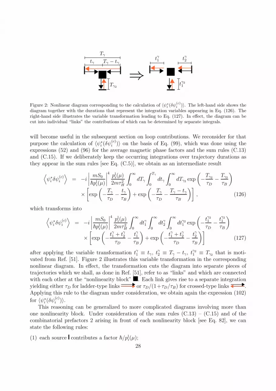
Figure 2: Nonlinear diagram corresponding to the calculation of 〈ψ∗

i(δψ

(c)i

)〉. The left-hand side shows thediagram together with the durations that represent the integration variables appearing in Eq. (126). Theright-hand side illustrates the variable transformation leading to Eq. (127). In effect, the diagram can becut into individual “links” the contributions of which can be determined by separate integrals.

will become useful in the subsequent section on loop contributions. We reconsider for thatpurpose the calculation of 〈ψ∗

i (δψ(c)i )〉 on the basis of Eq. (99), which was done using the

expressions (52) and (96) for the average magnetic phase factors and the sum rules (C.13)and (C.15). If we deliberately keep the occurring integrations over trajectory durations asthey appear in the sum rules [see Eq. (C.5)], we obtain as an intermediate result

⟨ψ∗i δψ

(c)i

⟩= −i

∣∣∣∣mS0

~pli(µ)

∣∣∣∣4pli(µ)

2mτ 2H

∫ ∞

0

dTγ

∫ Tγ

0

dtγ

∫ ∞

0

dTγ2 exp

(−Tγ2τD

− Tγ2τB

)

×[exp

(−TγτD

− tγτB

)+ exp

(−TγτD

− Tγ − tγτB

)], (126)

which transforms into

⟨ψ∗i δψ

(c)i

⟩= −i

∣∣∣∣mS0

~pli(µ)

∣∣∣∣4pli(µ)

2mτ 2H

∫ ∞

0

dtγ1

∫ ∞

0

dtγ2

∫ ∞

0

dtγ21 exp

(−t

γ21

τD− tγ21τB

)

×[exp

(−t

γ1 + tγ2τD

− tγ1τB

)+ exp

(−t

γ1 + tγ2τD

− tγ2τB

)](127)

after applying the variable transformation tγ1 ≡ tγ , tγ2 ≡ Tγ − tγ , t

γ21 ≡ Tγ2 that is moti-

vated from Ref. [51]. Figure 2 illustrates this variable transformation in the correspondingnonlinear diagram. In effect, the transformation cuts the diagram into separate pieces oftrajectories which we shall, as done in Ref. [51], refer to as “links” and which are connectedwith each other at the “nonlinearity block” . Each link gives rise to a separate integrationyielding either τD for ladder-type links or τD/(1+τD/τB) for crossed-type links .Applying this rule to the diagram under consideration, we obtain again the expression (102)

for 〈ψ∗i (δψ

(c)i )〉.

This reasoning can be generalized to more complicated diagrams involving more thanone nonlinearity block. Under consideration of the sum rules (C.13) – (C.15) and of thecombinatorial prefactors 2 arising in front of each nonlinearity block [see Eq. 82], we canstate the following rules:

(1) each source contributes a factor ~/pli(µ);

28

Figure 3: Relevant diagrams for the calculation of the nonlinear contribution to the backscattering proba-bility. Diagrams (a), (b), and (c) respectively correspond to the second, the third, and the fourth term onthe right-hand side of Eq. (104) as well as to the second, the third, and the fourth line of Eq. (128).

(2) each arrow emanating from a source contributes a factor S0 (and each conjugatearrow a factor S∗

0);

(3) each trajectory, scattering from lead to lead or ending at a nonlinearity event within thebilliard, contributes a factor m2/(~4τH);

(4) each nonlinearity event in the scattering wavefunction contributes a factor −ig~/m(and each nonlinearity event in the conjugate wavefunction contributes a factorig~/m);

(5) each ladder-type link contributes a factor τD;

(6) each crossed-type link contributes a factor (1/τD + 1/τB)−1.

Using these rules, we can re-calculate the crossed contribution c(g)ii to the retro-reflection

intensity. In contrast to Section 3.4, we do not explicitly need to introduce the nonlinearcrossed density C(g)(r) as done in Eq. (107). Instead, we directly sum over all possible com-binations of crossed diagrams as they are depicted in Fig. 3. Together with the contribution

29

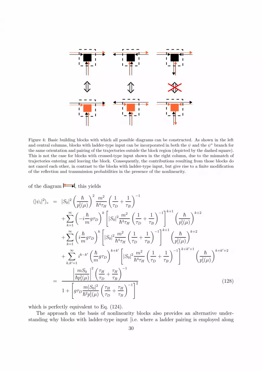
Figure 4: Basic building blocks with which all possible diagrams can be constructed. As shown in the leftand central columns, blocks with ladder-type input can be incorporated in both the ψ and the ψ∗ branch forthe same orientation and pairing of the trajectories outside the block region (depicted by the dashed square).This is not the case for blocks with crossed-type input shown in the right column, due to the mismatch oftrajectories entering and leaving the block. Consequently, the contributions resulting from those blocks donot cancel each other, in contrast to the blocks with ladder-type input, but give rise to a finite modificationof the reflection and transmission probabilities in the presence of the nonlinearity.

of the diagram , this yields

〈|ψi|2〉c = |S0|2(

~

pli(µ)

)2m2

~4τH

(1

τD+

1

τB

)−1

+

∞∑

k=1

(−i ~mgτD

)k[|S0|2

m2

~4τH

(1

τD+

1

τB

)−1]k+1(

~

pli(µ)

)k+2

+

∞∑

k=1

(i~

mgτD

)k[|S0|2

m2

~4τH

(1

τD+

1

τB

)−1]k+1(

~

pli(µ)

)k+2

+∞∑

k,k′=1

ik−k′(~

mgτD

)k+k′[|S0|2

m2

~4τH

(1

τD+

1

τB

)−1]k+k′+1(

~

pli(µ)

)k+k′+2

=

∣∣∣∣mS0

~pli(µ)

∣∣∣∣2(

τHτD

+τHτB

)−1

1 +

[gτD

m|S0|2~2pli(µ)

(τHτD

+τHτB

)−1]2 (128)

which is perfectly equivalent to Eq. (124).The approach on the basis of nonlinearity blocks also provides an alternative under-

standing why blocks with ladder-type input [i.e. where a ladder pairing is employed along

30

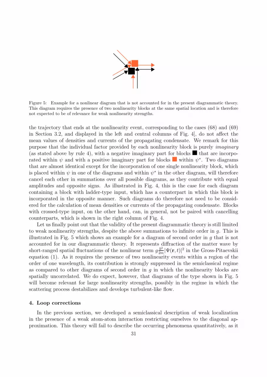
Figure 5: Example for a nonlinear diagram that is not accounted for in the present diagrammatic theory.This diagram requires the presence of two nonlinearity blocks at the same spatial location and is thereforenot expected to be of relevance for weak nonlinearity strengths.

the trajectory that ends at the nonlinearity event, corresponding to the cases (68) and (69)in Section 3.2, and displayed in the left and central columns of Fig. 4], do not affect themean values of densities and currents of the propagating condensate. We remark for thispurpose that the individual factor provided by each nonlinearity block is purely imaginary

(as stated above by rule 4), with a negative imaginary part for blocks that are incorpo-rated within ψ and with a positive imaginary part for blocks within ψ∗. Two diagramsthat are almost identical except for the incorporation of one single nonlinearity block, whichis placed within ψ in one of the diagrams and within ψ∗ in the other diagram, will thereforecancel each other in summations over all possible diagrams, as they contribute with equalamplitudes and opposite signs. As illustrated in Fig. 4, this is the case for each diagramcontaining a block with ladder-type input, which has a counterpart in which this block isincorporated in the opposite manner. Such diagrams do therefore not need to be consid-ered for the calculation of mean densities or currents of the propagating condensate. Blockswith crossed-type input, on the other hand, can, in general, not be paired with cancellingcounterparts, which is shown in the right column of Fig. 4.

Let us finally point out that the validity of the present diagrammatic theory is still limitedto weak nonlinearity strengths, despite the above summations to infinite order in g. This isillustrated in Fig. 5 which shows an example for a diagram of second order in g that is notaccounted for in our diagrammatic theory. It represents diffraction of the matter wave byshort-ranged spatial fluctuations of the nonlinear term g ~2

2m|Ψ(r, t)|2 in the Gross-Pitaevskii

equation (1). As it requires the presence of two nonlinearity events within a region of theorder of one wavelength, its contribution is strongly suppressed in the semiclassical regimeas compared to other diagrams of second order in g in which the nonlinearity blocks arespatially uncorrelated. We do expect, however, that diagrams of the type shown in Fig. 5will become relevant for large nonlinearity strengths, possibly in the regime in which thescattering process destabilizes and develops turbulent-like flow.

4. Loop corrections

In the previous section, we developed a semiclassical description of weak localizationin the presence of a weak atom-atom interaction restricting ourselves to the diagonal ap-proximation. This theory will fail to describe the occurring phenomena quantitatively, as it

31

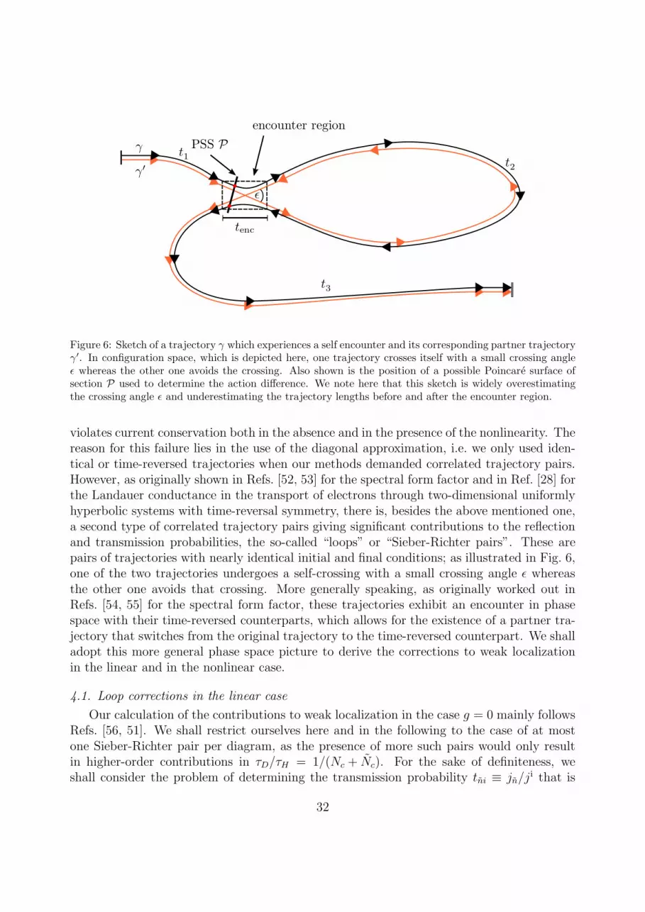
Figure 6: Sketch of a trajectory γ which experiences a self encounter and its corresponding partner trajectoryγ′. In configuration space, which is depicted here, one trajectory crosses itself with a small crossing angleǫ whereas the other one avoids the crossing. Also shown is the position of a possible Poincare surface ofsection P used to determine the action difference. We note here that this sketch is widely overestimatingthe crossing angle ǫ and underestimating the trajectory lengths before and after the encounter region.

violates current conservation both in the absence and in the presence of the nonlinearity. Thereason for this failure lies in the use of the diagonal approximation, i.e. we only used iden-tical or time-reversed trajectories when our methods demanded correlated trajectory pairs.However, as originally shown in Refs. [52, 53] for the spectral form factor and in Ref. [28] forthe Landauer conductance in the transport of electrons through two-dimensional uniformlyhyperbolic systems with time-reversal symmetry, there is, besides the above mentioned one,a second type of correlated trajectory pairs giving significant contributions to the reflectionand transmission probabilities, the so-called “loops” or “Sieber-Richter pairs”. These arepairs of trajectories with nearly identical initial and final conditions; as illustrated in Fig. 6,one of the two trajectories undergoes a self-crossing with a small crossing angle ǫ whereasthe other one avoids that crossing. More generally speaking, as originally worked out inRefs. [54, 55] for the spectral form factor, these trajectories exhibit an encounter in phasespace with their time-reversed counterparts, which allows for the existence of a partner tra-jectory that switches from the original trajectory to the time-reversed counterpart. We shalladopt this more general phase space picture to derive the corrections to weak localizationin the linear and in the nonlinear case.

4.1. Loop corrections in the linear case

Our calculation of the contributions to weak localization in the case g = 0 mainly followsRefs. [56, 51]. We shall restrict ourselves here and in the following to the case of at mostone Sieber-Richter pair per diagram, as the presence of more such pairs would only resultin higher-order contributions in τD/τH = 1/(Nc + Nc). For the sake of definiteness, weshall consider the problem of determining the transmission probability tni ≡ jn/j

i that is

32

associated with the scattering process from the incident channel i in the left lead to the finalchannel n in the right lead. Our purpose is therefore to calculate

⟨|ψ(0)

n |2⟩=

∣∣∣∣∣S0π~√WW

∣∣∣∣∣

2 ∑

ν1,ν′1=±1

∑

ν2,ν′2=±1

ν1ν′1ν2ν

′2

⟨G(zν1n , z

ν′1

i , µ)G

∗ (zν2n , z

ν′2

i , µ)⟩

. (129)

As this quantity involves a product of two Green functions, we are concerned with sumsover pairs of classical trajectories γ, γ′ here. In the context of the diagonal approximation,we already evaluated in Section 3 the most dominant contribution to this transmissionprobability, for which γ′ is identical to γ.

The next group of systematically correlated trajectories consists of pairs γ, γ′ that ex-hibit, as sketched in Fig. 6, a self-encounter in phase space [52, 28, 51]. Their action differencecan be determined by defining a Poincare surface of section P within the encounter region,which is oriented perpendicular to γ on the first passage of this trajectory through it, i.e.,which is pierced by the first stretch of γ at its origin. Linearizing the classical dynamicsin the vicinity of this trajectory, we can define two basis vectors es and eu within the two-dimensional surface of section P that are respectively oriented along the stable and unstablemanifold of γ. The action difference between γ and γ′ is then evaluated as [54, 55]

∆Sγ,γ′≡Sγ − Sγ′ = su (130)

where s and u denote the coordinates with respect to the basis vectors es and eu, respectively,at which the trajectory γ pierces through P for the second time. Obviously, ∆Sγ,γ′ can besufficiently small, i.e. of the order of ~, if, as depicted in Fig. 6, one of the two trajectoriesexhibits a self-crossing in configuration space with a very small crossing angle ǫ [52, 28].The partner trajectory, whose existence and uniqueness is granted by the chaoticity of theclassical dynamics, will then avoid that self-crossing and follow the loop in between the twopiercings through P in the opposite direction.

In order to evaluate the contributions of such Sieber-Richter pairs to Eq. (129), weneed to determine the probability of a trajectory γ to exhibit a near-encounter in phasespace. Due to ergodicity, the probability density for the trajectory γ to pierce again throughthe Poincare surface of section in the opposite direction at given coordinates s and u andafter a given propagation time t2 after the first piercing is given by the Liouville measureδ[µ−H0(p,q)]/Σ(µ) with (p,q) the coordinates of the second piercing in the full phasespace and Σ(µ)≡

∫d2q′

∫d2p′δ[µ−H0(p

′,q′)] the phase-space volume of the energy shell. Ifwe want to calculate the probability density for a trajectory γ with a given total propagationtime T to have a partner trajectory γ′ with a given action difference ∆Sγ,γ′ ≡ ∆S, we aretempted to integrate this Liouville measure over all “intermediate” propagation times t2between the first and the second intersection through the Poincare surface of section P, overall “initial” propagation times t1 from the incident channel to the first intersection through P,over all “final” propagation times t3 from the second intersection through P to the outgoingchannel, as well as over all possible phase-space coordinates s, u that γ exhibits within Pat its second piercing, with the requirements that su = ∆S and t1 + t2 + t3 = T . This naıve

33

integration would, however, lead to multiple countings of such trajectory pairs. Indeed, theplacement of the Poincare surface of section P is not unique, but can be shifted along thefirst stretch of the trajectory γ. This generally will lead to different coordinates s, u of thesecond stretch of γ when passing through P, but the product su of these coordinates will notchange, provided the second piercing point of γ is also in a sufficiently close neigbourhoodof the origin of P such that the linearization of the classical dynamics around γ is still valid(see also the calculations in Appendix Appendix E).

The contribution of an individual Sieber-Richter pair with an action difference ∆S would,when performing the above-mentioned integration, therefore effectively be overweighted bya factor tenc ≡ tenc(∆S) that corresponds to the typical “duration” of the encounter, i.e., thetypical propagation time within which one of the trajectories “sees” the other one within adistance that is within the linearization region of its transverse dynamics. Defining by λ theLyapunov exponent of the ergodic system [57], and introducing c as the maximal distancealong the stable and unstable manifolds es, eu for the linearization of the transverse dynamicswithin the Poincare surface of section P to be valid (i.e., we require that −c < s, u < c; theprecise value of c, which is related to the Ehrenfest time of the system as pointed out inAppendix Appendix E.1, will not be of relevance in the end), we can define [56, 51]

tenc(su) =1

λln

(c2

|su|

). (131)

This duration tenc(su) reflects the fact that some minimal time is needed for the two nearbytrajectory stretches to part from each other, in order to form the loop on one end and toexit toward different leads on the other end of the encounter region.

In view of these considerations, we define (see also Ref. [51])

w(∆S, t2;T ) =

∞∫

0

∞∫

0

dt1dt3

c∫

−c

c∫

−c

dsduδ(su−∆S)

Σ(µ)tenc(su)δ[t1 + t2 + t3 + 2tenc(su)− T ] (132)

as the probability density for a trajectory γ with the total propagation time T to have apartner trajectory γ′ with an action difference ∆S and a loop duration t2. This loop durationt2 as well as the initial and final propagation times t1 and t3 that appear in the integrations inEq. (132) are, as illustrated in Fig. 6, defined not with respect to the particular placement ofthe Poincare surface of section, but with respect to the location of the encounter region along

the trajectory. Using Aγ≃Aγ′ and µγ≃µγ′ for the trajectory pair γ, γ′, the loop contributions

to 〈|ψ(0)n |2〉 are calculated as

⟨∣∣∣ψ(0)n

∣∣∣2⟩

loop

=|S0|2 (π~)2WW

∑

ν,ν′=±1

∫ ∞

−∞

d(∆S)

∫ ∞

0

dt2∑

γ

⟨∣∣∣Aγ

(zνn, z

ν′

i , µ)∣∣∣

2⟩

×w(∆S, t2;Tγ) exp(i

~∆S

)exp

(− t2τB

), (133)

34

where the dephasing factor exp(−t2/τB) originates from ϕγ [rγ(t1 + tenc + t2), rγ(t1 + tenc), µ],the flux integral along the loop according to Eq. (52). We neglect here the contribution ofthe flux inside the encounter region, which will be discussed in the next subsection.

When applying the sum rule (C.15), we have to use a modified survival probabilityexp [−(T − tenc)/τd] in Eq. (C.6). Indeed, if the first stretch of the encounter lies within thebilliard, the second one does so as well, thus the trajectory does not risk to escape during itssecond passing through the encounter region. The relevant time for the survival probabilityhas therefore to be reduced by the duration tenc of this second stretch. We then obtain⟨∣∣∣ψ(0)

n

∣∣∣2⟩

loop

=

∣∣∣∣mS0

~

∣∣∣∣2

1

τHpln(µ)pli(µ)

∫ ∞

0

dt1

∫ ∞

0

dt2

∫ ∞

0

dt3 exp

(−t1 + t2 + t3

τD− t2τB

)

×∫ c

−c

ds

∫ c

−c

du1

Σ(µ)tenc(su)exp

(i

~su

)exp

(−tenc(su)

τD

)

= − m

pln(µ)ji(τDτH

)21

1 + τD/τB, (134)

as shown in Appendix Appendix E.1. In a similar way as for nonlinearity blocks (seethe discussion in Section 3.5), the encounter region cuts the diagram into three ”links”contributing either τD or τD/(1 + τD/τB).

The same derivation can be applied in order to calculate the loop contributions to thereflection probability into channel n, leading to exactly the same result as in Eq. (134). Wetherefore obtain

δ(t(0)ni

)loop= δ

(r(0)ni

)loop= −

(τDτH

)21

1 + τD/τB(135)

as loop contributions to the reflection and transmission probabilities r(0)ni and t

(0)ni in the

absence of interaction. These corrections do indeed restore current conservation in leadingsemiclassical order. Combining all ladder, crossed, and loop contributions that are evaluatedin Eqs. (42), (57), and (135), respectively, we obtain with Eq. (44)

r(0)ii =

τDτH

(1 +

τH − τDτH

1

1 + τD/τB

)=

1

Nc + Nc

(1 +

Nc + Nc − 1

Nc + Nc

1

1 +B2/B20

)(136)

for the probability of retro-reflection into the incident channel n = i, as well as

r(0)ni = t

(0)ni =

τDτH

(1− τD

τH

1

1 + τD/τB

)=

1

Nc + Nc

(1− 1

Nc + Nc

1

1 +B2/B20

)(137)

for the probabilities of reflection into a different channel n 6= i and of transmission intochannel n. This yields the total reflection and transmission probabilities

R(0) =Nc

Nc + Nc

+Nc

(Nc + Nc)21

1 +B2/B20

, (138)

T (0) =Nc

Nc + Nc

− Nc

(Nc + Nc)21

1 +B2/B20

, (139)

in the linear case g = 0, which obviously satify R(0) + T (0) = 1.

35

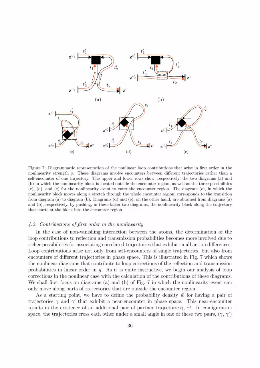
Figure 7: Diagrammatic representation of the nonlinear loop contributions that arise in first order in thenonlinearity strength g. These diagrams involve encounters between different trajectories rather than aself-encounter of one trajectory. The upper and lower rows show, respectively, the two diagrams (a) and(b) in which the nonlinearity block is located outside the encounter region, as well as the three possibilities(c), (d), and (e) for the nonlinearity event to enter the encounter region. The diagram (c), in which thenonlinearity block moves along a stretch through the whole encounter region, corresponds to the transitionfrom diagram (a) to diagram (b). Diagrams (d) and (e), on the other hand, are obtained from diagrams (a)and (b), respectively, by pushing, in these latter two diagrams, the nonlinearity block along the trajectorythat starts at the block into the encounter region.

4.2. Contributions of first order in the nonlinearity

In the case of non-vanishing interaction between the atoms, the determination of theloop contributions to reflection and transmission probabilities becomes more involved due toricher possibilities for associating correlated trajectories that exhibit small action differences.Loop contributions arise not only from self-encounters of single trajectories, but also fromencounters of different trajectories in phase space. This is illustrated in Fig. 7 which showsthe nonlinear diagrams that contribute to loop corrections of the reflection and transmissionprobabilities in linear order in g. As it is quite instructive, we begin our analysis of loopcorrections in the nonlinear case with the calculation of the contributions of these diagrams.We shall first focus on diagrams (a) and (b) of Fig. 7 in which the nonlinearity event canonly move along parts of trajectories that are outside the encounter region.

As a starting point, we have to define the probability density w for having a pair oftrajectories γ and γ′ that exhibit a near-encounter in phase space. This near-encounterresults in the existence of an additional pair of partner trajectoriesγ, γ′. In configurationspace, the trajectories cross each other under a small angle in one of these two pairs, (γ, γ′)

36

Figure 8: Three different constellations for the stretches involved in an encounter region. In the case ofconstellation (a), which arises also in the linear case discussed in Section 4.1, the encounter region itself doesnot provide a significant contribution to the dephasing in the presence of an external magnetic field, sincethe flux integrals in the phases associated with the individual stretches cancel each other. This is differentfor the constellations (b) and (c) in which twice (b) and four times (c) the flux integral from a stretch ofduration tenc remains, yielding the phase factors exp(−tenc/τB) for constellation (b) and exp(−2tenc/τB) forconstellation (c).

or (γ, γ′), whereas the other pair avoids this crossing.The probability density w is specified for a given action difference ∆S between the trajec-

tories γ, γ′ and the pair of partner trajectories γ, γ′, as well as for given partial propagationtimes t, t′ of the trajectories γ and γ′, respectively, before (in the case of trajectory γ) orafter (in the case of trajectory γ′) the encounter region, which may become relevant forthe evaluation of magnetic dephasing. It furthermore depends parametrically on the totalpropagation times T and T ′ of the two trajectories γ, γ′ as well as on the orientations of theindividual trajectory stretches within the encounter region, as these orientations might giverise to additional contributions to the magnetic dephasing. Figure 8 displays three differentpossibilities for orienting the trajectory stretches within the encounter region. While the en-counter region in constellation (a) does not contribute to the dephasing in the presence of amagnetic field, the constellations (b) and (c) contribute with phase factors exp(−tenc/τB) andexp(−2tenc/τB), respectively, as there are one (b) and two (c) trajectory stretchesof the linear Green function that are not balanced by the complex conjugate counterparts

.Denoting by n ∈ 0, 1, 2 the number of imbalanced pairs of stretches within the en-

counter region, we define

w(∆S, t, t′;T, T ′, n) =

∫ ∞

0

∫ ∞

0

dtdt′∫ c

−c

∫ c

−c

dsduδ (∆S − su)

Σ(µ)tenc(su)exp

[−ntenc(su)

τB

]

×δ(t+ t + tenc(su)− T

)δ(t′ + t′ + tenc(su)− T ′

)(140)

as the density of trajectory pairs γ, γ′ that come close to each other in phase space andthus have partner trajectories with a combined action difference ∆S. In this expression, theintegration variables t and t′ correspond to the propagation times of the final and initialparts of the trajectories γ and γ′, respectively, after leaving (t) and before entering (t′) theencounter region. We have n = 0 ≡ na for diagram (a) and n = 1 ≡ nb for diagram (b) inFig. 7.

37

Calculating now the contributions of the diagrams shown in the upper row of Fig. 7(which are multiplied by a combinatorial factor 2 as there are two possibilities to constructthese diagrams), we obtain

⟨ψ

(0)∗n

(δψ

(1)n

)⟩loop, (a/b)

= 2~2

2m

|S0|4 (π~)3

WW 2

⟨∑

ν′1,ν′

2,ν=±1

G∗ (

zνn, zν′1

i , µ)

×∫

Ω

d2r′G (zνn, r′, µ)G

(r′, z

ν′1

i , µ)G(r′, z

ν′2

i , µ)G

∗(r′, z

ν′2

i , µ)⟩

loop, (a/b)

= 2~2

2m

|S0|4 (π~)3

WW 2

∫ ∞

−∞

d(∆S)

∫ ∞

0

dt1

∫ ∞

0

dt′2∑

ν′1,ν′

2,ν=±1

∑

γ′

⟨∣∣∣Aγ′

(zν′2

i , zν′1

i , µ)∣∣∣

2⟩

×(− i

~

)∫ ∞

0

dt′1∑

γ

⟨∣∣∣Aγ [zνn, rγ′ (t′1) , µ]

∣∣∣2⟩

×w(∆S, t1, t

′2;Tγ , Tγ′−t′1, na/b

)exp

(i

~∆S

)exp

(−t1 + t′2

τB

)

= −i m

pln(µ)

(m |S0|2~2pli(µ)

)21

τ 2H

∫ ∞

0

dt′1

∫ ∞

0

dt′2

∫ ∞

0

dt′3

∫ ∞

0

dt1

∫ ∞

0

dt2

× exp

(−t

′1 + t′2 + t′3 + t1 + t2

τD− t1 + t′2

τB

)

×∫ c

−c

ds

∫ c

−c

du1

Σ(µ)tenc(su)exp

(i

~su

)exp

[−tenc(su)

τD−na/b

tenc(su)

τB

], (141)

where we applied the sum rules (C.14, C.15) to convert the sums over classical trajectoriesγ, γ′ into integrations over trajectory durations Tγ, Tγ′ , taking into account that we haveto use a reduced effective time Tγ + Tγ′ − tenc for the classical survival probability. Gaugeinvariance of the result is ensured by the fact that the encounter region closes the overallflux integral. The integration over s and u is calculated in Appendix Appendix E.1 andyields −1/(τDτH) for n = na = 0 as well as − (1 + τD/τB) /(τDτH) for n = nb = 1. Wetherefore obtain

⟨ψ

(0)∗n

(δψ

(1)n

)⟩loop, (a)

= im

pln(µ)

(ji)2(τDτH

)3

τD

(1

1 + τD/τB

)2

, (142)

⟨ψ

(0)∗n

(δψ

(1)n

)⟩loop, (b)

= im

pln(µ)

(ji)2(τDτH

)3

τD

(1

1 + τD/τB

)(143)

for the cases where the nonlinearity block is located outside the encounter region.As shown in the lower row of Fig. 7, there are two qualitatively different possibilities

for the nonlinearity event to enter the encounter region. In the first scenario, depicted inFig. 7(c), the nonlinearity event moves along a trajectory that provides a stretch within theencounter region. This scenario corresponds to the transition from diagram (a) to diagram

38

(b). Its contribution is calculated as⟨ψ

(0)∗n

(δψ

(1)n

)⟩loop, (c)

=

= 2~2

2m

|S0|4 (π~)3

WW 2

∫ ∞

−∞

d(∆S)

∫ ∞

0

dt1

∫ ∞

0

dt′1∑

ν′1,ν′

2,ν=±1

∑

γ′

⟨∣∣∣Aγ′

(zν′2

i , zν′1

i , µ)∣∣∣

2⟩

×(− i

~

)∫ tenc(∆S)

0

dt′∑

γ

⟨∣∣∣Aγ [zνn, rγ′(t′1+t

′), µ]∣∣∣2⟩

×w (∆S, t1, t′1;Tγ , Tγ′, 0) exp

(i

~∆S

)exp

(−t1 + t′

τB

)

= −i m

pln(µ)

(ji)2 1

τ 2H

∫ ∞

0

dt′1

∫ ∞

0

dt′2

∫ ∞

0

dt1

∫ ∞

0

dt2

× exp

(−t

′1 + t′2 + t1 + t2

τD− t1 + t′2

τB

)

×∫ c

−c

ds

∫ c

−c

du1

Σ(µ)tenc(su)exp

(i

~

)exp

(−tenc(su)

τD

)∫ tenc(su)

0

dt′ exp

(− t′

τB

)

= −i m

pln(µ)

(ji)2(τDτH

)3

τD

(1

1 + τD/τB

)= −

⟨ψ

(0)∗n

(δψ

(1)n

)⟩loop, (b)

(144)

[see Fig. 7(c) for the signification of t1, t2, t′1, t

′2], where the integrations over s, u and over

the propagation time t′ within the encounter region (whose gauge field dependence is takeninto account in the integration) yield, as shown in Appendix Appendix E.2, 1/τH .

In the other scenario, depicted in Fig. 7(d) and (e), a trajectory pair leaving the encounterand ending at a nonlinearity event becomes arbitrarily small until finally the nonlinearityevent enters the encounter region but does not traverse it. This case requires a modificationof the probability density of suitable partner trajectories as some stretches do not leave theencounter region any more but terminate at a certain point within it. Following Refs. [58,59, 60], we define a reduced encounter region with the duration

tenc(t′, u) ≡ t′ +

1

λln

(c

|u|

)(145)

where t′ ∈ [0, (1/λ) ln(c/|s|)] is the time interval between the nonlinearity event and thePoincare surface of section P that is optimally chosen to be located in the center of theencounter region. As a consequence, we have to extend the integration over s and u, asso-ciated with the possible action differences su, by an integration over all possible time spanst′ defining the location of the nonlinearity event with respect to P, which substitutes one ofthe integrations over time in Eq. (140). This yields the modified probability density

w(∆S, t, t′;T, T ′, n) =

∫ c

−c

∫ c

−c

dsdu

∫ ∞

0

dt

∫ (1/λ) ln(c/|s|)

0

dt′δ (∆S − su)

Σ(µ)tenc(t′, u)exp

(−ntenc(t

′, u)

τB

)

×δ[t + t+ tenc(t

′, u)− T]δ[t′ + tenc(t

′, u)− T ′]. (146)

39

Using this density for the calculation of diagram (d) in Fig. 7, we obtain

⟨ψ

(0)∗n

(δψ

(1)n

)⟩loop, (d)

=

= 2~2

2m

|S0|4 (π~)3

WW 2

∫ ∞

−∞

d(∆S)

∫ ∞

0

dt2

∫ ∞

0

dt′2∑

ν′1,ν′

2,ν=±1

∑

γ′

⟨∣∣∣Aγ′

(zν′2

i , zν′1

i , µ)∣∣∣

2⟩

×(− i

~

)∫ ∞

0

dt′1∑

γ

⟨∣∣∣Aγ [zνn, rγ′ (t′1) , µ]

∣∣∣2⟩

×w (∆S, t2, t′2;Tγ, Tγ′−t′1, 0) exp

(i

~∆S

)exp

(− t′2τB

)

= −i m

pln(µ)

(ji)2 1

τ 2H

∫ ∞

0

dt2

∫ ∞

0

dt′2

∫ ∞

0

dt′1

∫ ∞

0

dt′3 exp

(−t

′1 + t′2 + t′3 + t2

τD− t′2τB

)

×∫ c

−c

ds

∫ c

−c

du

∫ (1/λ) ln(c/|s|)

0

dt11

Σ(µ)tenc(t1, u)exp

(i

~su

)exp

(− tenc(t1, u)

τD

)

= −i m

pln(µ)

(ji)2(τDτH

)3

τD

(1

1 + τD/τB

)=⟨ψ

(0)∗n

(δψ

(1)n

)⟩

loop, (c)(147)

where we evaluate the integration over s, u and t1 in Appendix Appendix E.2 yielding 1/τH .The calculation of the contribution of diagram (e) in Fig. 7 proceeds in perfect analogy withthe one presented for diagram (d) and yields the same result

⟨ψ

(0)∗n

(δψ

(1)n

)⟩

loop, (e)= −i m

pln(µ)

(ji)2(τDτH

)3

τD

(1

1 + τD/τB

)=⟨ψ

(0)∗n

(δψ

(1)n

)⟩

loop, (c).

(148)

The overall nonlinear loop contribution to 〈ψ(0)∗n (δψ

(1)n )〉 originating from the diagrams

shown in Fig. 7 therefore sums up to

⟨ψ

(0)∗n

(δψ

(1)n

)⟩

loop= i

m

pln(µ)

(ji)2(τDτH

)3

τD

[(1

1 + τD/τB

)2

− 2

(1

1 + τD/τB

)]. (149)

As this expression is purely imaginary, no modifications of transmission and reflection prob-abilities are expected in linear order in the interaction strength g, which is in perfect accor-dance with the discussion in Section 3.4 [see Eq. (102)].

4.3. Contributions of arbitrary order in the nonlinearity

As we can see from the above calculations, the presence of an encounter region perfectlyfits to the picture of diagrams consisting of separated parts, which was developed in Section3.5, since we can perform the integrations corresponding to an encounter region indepen-dently from the remaining integrations over link durations. Encounter regions can, in thespirit of Section 3.5, be interpreted as extended “blocks” which are connected via four linksto other (nonlinearity or encounter) blocks as well as to the leads of the system. Care must

40

be taken, though, if a nonlinearity block enters the encounter region, as is the case in thediagrams depicted in the lower row of Fig. 7. Under consideration of the calculations per-formed in Appendix Appendix E, we can extend our diagrammatic rules listed in Section3.5 by the following ones:

(7) each encounter region containing no nonlinearity event contributes a factor −(1 +nτB/τD)/(τDτH) where n = 0, 1, 2 counts the number of trajectory pairs with im-balanced stretches within the encounter region (see Fig. 8);

(8) each encounter region including a nonlinearity event contributes a factor 1/τH .

As was already argued in Section 3.5, diagrams containing a nonlinearity block with ladder-type input (as the ones shown in the left and central column of Fig. 4) will not contribute tothe reflection and transmission probabilities as they are cancelled by counterparts in whichthis nonlinearity block is attached to the complex conjugate trajectory stretch. We cantherefore restrict ourselves to “crossed type” nonlinearity blocks shown in the right columnin Fig. 4.

Figure 9 shows the complete set of nonlinear diagrams contributing to reflection andtransmission probabilities in arbitrary order in the nonlinearity strength g. These diagramsconsist of the same chains of nonlinearity blocks as the ones shown in Fig. 3, with themain difference that these chains cannot be directly attached to a lead as we are calculatingthe scattering amplitude to an arbitrary (i.e., not necessarily the incident) channel in thereflected or transmitted lead; instead, they have to be connected to ladder links via anencounter region. In perfect analogy with Fig. 7, the nonlinearity blocks at the right endsof the chains in the diagrams (a), (b), (d), and (e) can be moved all the way through theentire encounter region, thereby giving rise to a transition from diagram (a) to diagram (b)as well as from diagram (d) to diagram (e). The other blocks located at the ends of thechains in the diagrams (a) – (g) can, in analogy with the diagrams (d) and (e) of Fig. 7, bepushed into the encounter region by moving them along the trajectories that start or endat those blocks.

Using the diagrammatic rules (1) – (8) stated in Section 3.5 and above, the contributionsof these relevant diagrams as well as their corrections due to nonlinearity events enteringthe encounter region are straightforwardly evaluated. Defining by

g0 ≡(jiτDc

(0)ii

)−1

=

(jiτD

τDτH

1

1 + τD/τB

)−1

(150)

the relevant scale for the nonlinearity strength appearing in Eq. (124), we obtain for the

41

Figure 9: Complete set of diagrams of k-th order in g containing one encounter region and k nonlinearityblocks of the “crossed” type shown in the right column of Fig. 4 which are located outside the encounter

region. The diagrams (a) - (f) are contributions coming from 〈ψ(0)∗n

(δψ(k)n

)〉 and 〈(δψ(k)∗n

)ψ(0)n

〉, respectively,where (c) and (f) only exist for k ≥ 2. Contrary to the other diagrams, (g) is contained in 〈(δψ(k1)∗

n)(δψ

(k2)n

)〉with k1 + k2 = k and k1, k2 ≥ 1. As is shown in Eq. (158), the contributions of the diagrams (b), (c), (e),and (f) exactly cancel each other.

42

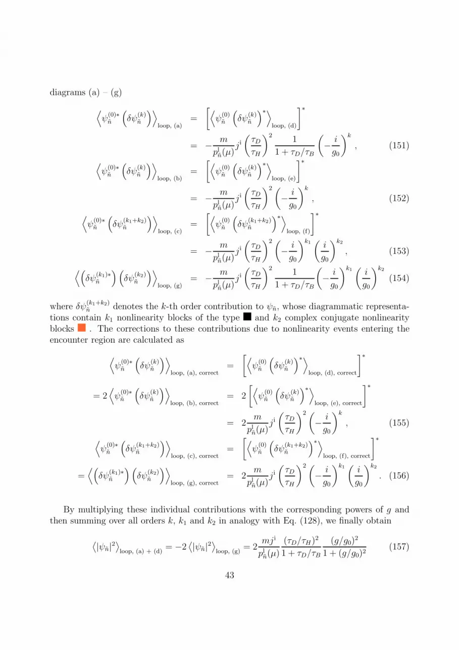
diagrams (a) – (g)

⟨ψ

(0)∗n

(δψ

(k)n

)⟩loop, (a)

=

[⟨ψ

(0)n

(δψ

(k)n

)∗⟩loop, (d)

]∗

= − m

pln(µ)ji(τDτH

)21

1 + τD/τB

(− i

g0

)k

, (151)

⟨ψ

(0)∗n

(δψ

(k)n

)⟩loop, (b)

=

[⟨ψ

(0)n

(δψ

(k)n

)∗⟩loop, (e)

]∗

= − m

pln(µ)ji(τDτH

)2(− i

g0

)k

, (152)

⟨ψ

(0)∗n

(δψ

(k1+k2)n

)⟩loop, (c)

=

[⟨ψ

(0)n

(δψ

(k1+k2)n

)∗⟩loop, (f)

]∗

= − m

pln(µ)ji(τDτH

)2(− i

g0

)k1 ( i

g0

)k2

, (153)

⟨(δψ

(k1)∗n

)(δψ

(k2)n

)⟩

loop, (g)= − m

pln(µ)ji(τDτH

)21

1 + τD/τB

(− i

g0

)k1 ( i

g0

)k2

(154)

where δψ(k1+k2)n denotes the k-th order contribution to ψn, whose diagrammatic representa-

tions contain k1 nonlinearity blocks of the type and k2 complex conjugate nonlinearityblocks . The corrections to these contributions due to nonlinearity events entering theencounter region are calculated as

⟨ψ

(0)∗n

(δψ

(k)n

)⟩

loop, (a), correct=

[⟨ψ

(0)n

(δψ

(k)n

)∗⟩

loop, (d), correct

]∗

= 2⟨ψ

(0)∗n

(δψ

(k)n

)⟩loop, (b), correct

= 2

[⟨ψ

(0)n

(δψ

(k)n

)∗⟩loop, (e), correct

]∗

= 2m

pln(µ)ji(τDτH

)2(− i

g0

)k

, (155)

⟨ψ

(0)∗n

(δψ

(k1+k2)n

)⟩loop, (c), correct

=

[⟨ψ

(0)n

(δψ

(k1+k2)n

)∗⟩loop, (f), correct

]∗

=⟨(δψ

(k1)∗n

)(δψ

(k2)n

)⟩loop, (g), correct

= 2m

pln(µ)ji(τDτH

)2(− i

g0

)k1 ( i

g0

)k2

. (156)

By multiplying these individual contributions with the corresponding powers of g andthen summing over all orders k, k1 and k2 in analogy with Eq. (128), we finally obtain

⟨|ψn|2

⟩loop, (a) + (d)

= −2⟨|ψn|2

⟩loop, (g)

= 2mji

pln(µ)

(τD/τH)2

1 + τD/τB

(g/g0)2

1 + (g/g0)2(157)

43

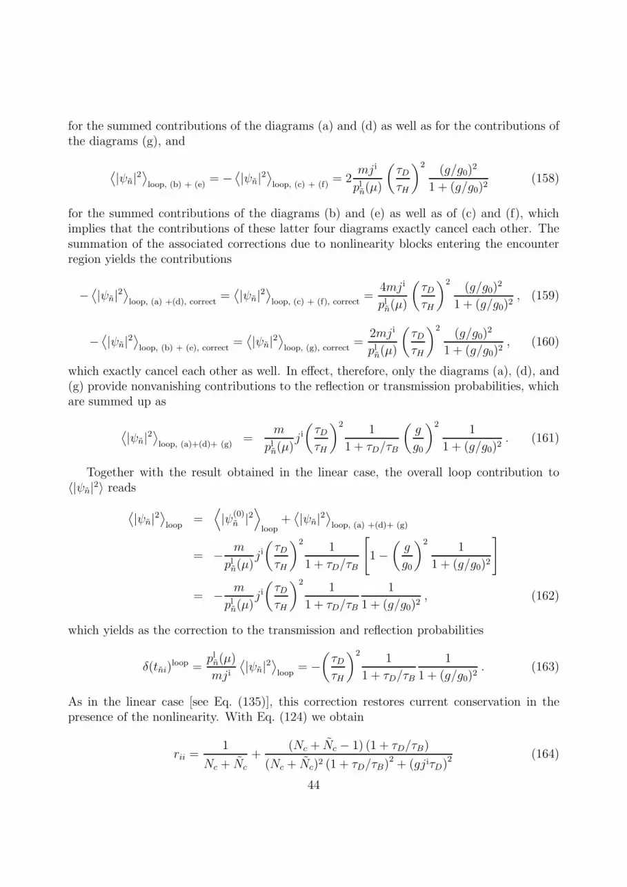
for the summed contributions of the diagrams (a) and (d) as well as for the contributions ofthe diagrams (g), and

⟨|ψn|2

⟩loop, (b) + (e)

= −⟨|ψn|2

⟩loop, (c) + (f)

= 2mji

pln(µ)

(τDτH

)2(g/g0)

2

1 + (g/g0)2(158)

for the summed contributions of the diagrams (b) and (e) as well as of (c) and (f), whichimplies that the contributions of these latter four diagrams exactly cancel each other. Thesummation of the associated corrections due to nonlinearity blocks entering the encounterregion yields the contributions

−⟨|ψn|2

⟩loop, (a) +(d), correct

=⟨|ψn|2

⟩loop, (c) + (f), correct

=4mji

pln(µ)

(τDτH

)2(g/g0)

2

1 + (g/g0)2, (159)

−⟨|ψn|2

⟩loop, (b) + (e), correct

=⟨|ψn|2

⟩loop, (g), correct

=2mji

pln(µ)

(τDτH

)2(g/g0)

2

1 + (g/g0)2, (160)

which exactly cancel each other as well. In effect, therefore, only the diagrams (a), (d), and(g) provide nonvanishing contributions to the reflection or transmission probabilities, whichare summed up as

⟨|ψn|2

⟩loop, (a)+(d)+ (g)

=m

pln(µ)ji(τDτH

)21

1 + τD/τB

(g

g0

)21

1 + (g/g0)2. (161)

Together with the result obtained in the linear case, the overall loop contribution to〈|ψn|2〉 reads

⟨|ψn|2

⟩loop

=⟨|ψ(0)

n |2⟩loop

+⟨|ψn|2

⟩loop, (a) +(d)+ (g)

= − m

pln(µ)ji(τDτH

)21

1 + τD/τB

[1−

(g

g0

)21

1 + (g/g0)2

]

= − m

pln(µ)ji(τDτH

)21

1 + τD/τB

1

1 + (g/g0)2, (162)

which yields as the correction to the transmission and reflection probabilities

δ(tni)loop =

pln(µ)

mji⟨|ψn|2

⟩loop

= −(τDτH

)21

1 + τD/τB

1

1 + (g/g0)2. (163)

As in the linear case [see Eq. (135)], this correction restores current conservation in thepresence of the nonlinearity. With Eq. (124) we obtain

rii =1

Nc + Nc

+(Nc + Nc − 1) (1 + τD/τB)

(Nc + Nc)2 (1 + τD/τB)2 + (gjiτD)

2 (164)

44

for the probability of retro-reflection into the incident channel n = i, as well as

rni = tni =1

Nc + Nc

− 1 + τD/τB

(Nc + Nc)2 (1 + τD/τB)2 + (gjiτD)

2 (165)

for the probability rni of reflection into a different channel n 6= i of the incident lead andfor the probability tni of transmission into channel n. This yields the total reflection andtransmission probabilities

R =Nc

Nc + Nc

+Nc (1 + τD/τB)

(Nc + Nc)2 (1 + τD/τB)2 + (gjiτD)

2 , (166)

T =Nc

Nc + Nc

− Nc (1 + τD/τB)

(Nc + Nc)2 (1 + τD/τB)2 + (gjiτD)

2 , (167)

which obviously satify R + T = 1.

5. Comparison with numerical results

Figures 10 and 11 display (in their right columns) the semiclassical prediction (164) forthe probability of retro-reflection into the incident channel as evaluated for the billiards a andb, respectively, that are shown in Fig. 1. The sizes of the two billiards are chosen such thatboth the incident and the transmitted leads exhibit five open channels, i.e. Nc = Nc = 5, atthe energy that corresponds to the chemical potential µ of the incident beam. We specificallyhave the areas Ω ≃ 3.41 × 103 ~2/(mµ0) for billiard a and Ω ≃ 3.29 × 103 ~2/(mµ0) forbilliard b, where µ0 defines the characteristic energy scale for the chemical potential of theatomic beam (i.e. we choose µ = µ0 for the evaluation of the semiclassical retro-reflectionprobability). The incident current is chosen as ji = 1.0µ0/~. As described in AppendixAppendix D, the dwell time τD and the characteristic scale B0 of the effective magnetic fieldwere classically determined from the numerically computed length and area distributionswithin the two billiards, respectively; we obtained jiτD ≃ 267 and B0 ≃ 1.55×10−3mµ0/~ ≃0.844 × 2π~/Ω for billiard a as well as jiτD ≃ 241 and B0 ≃ 4.21 × 10−4mµ0/~ ≃ 0.221 ×2π~/Ω for billiard b.

In the linear case g = 0, a Lorentzian peak is obtained for the retro-reflection probabilityas a function of the effective magnetic field, on top of an incoherent background at rii ≃1/(Nc + Nc) = 0.1. This is the characteristic signature of weak localization. As is evidentfrom Eq. (164), the presence of a finite nonlinearity g gives rise to a reduction of the coherentenhancement of the backscattering probability, which ultimately approaches the incoherentbackground 1/(Nc+ Nc) for g → ∞. This reduction, however, is more effective at the centerof the backscattering peak than in its wings, such that for intermediate values of g a localminimum may be encountered in the reflection probability around B = 0.

This prediction is indeed confirmed by numerical computations of the quasi-stationarytransport process within the two billiards under consideration. As explicit numerical propa-gations of the time-dependent Gross-Pitaevskii equation (5) are rather time-consuming, weuse, in practice, a different approach in order to compute the scattering states of the system.

45

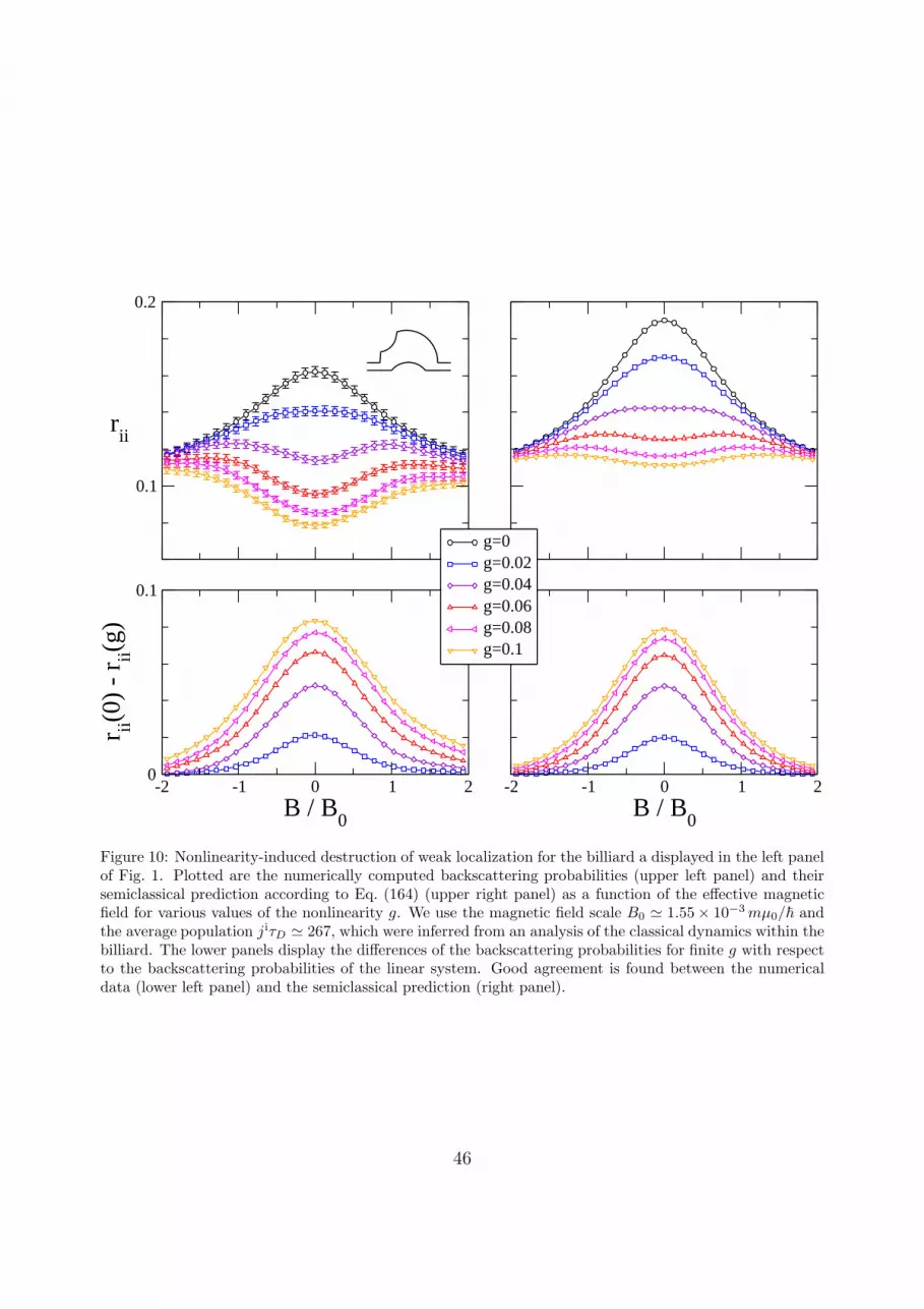
0.1

0.2

rii

g=0g=0.02g=0.04g=0.06g=0.08g=0.1

g=0g=0.02g=0.04g=0.06g=0.08g=0.1

-2 -1 0 1 2B / B

0

0

0.1

r ii(0)

- r ii(g

)

g=0g=0.02g=0.04g=0.06g=0.08g=0.1

-2 -1 0 1 2B / B

0

g=0g=0.02g=0.04g=0.06g=0.08g=0.1

Figure 10: Nonlinearity-induced destruction of weak localization for the billiard a displayed in the left panelof Fig. 1. Plotted are the numerically computed backscattering probabilities (upper left panel) and theirsemiclassical prediction according to Eq. (164) (upper right panel) as a function of the effective magneticfield for various values of the nonlinearity g. We use the magnetic field scale B0 ≃ 1.55× 10−3mµ0/~ andthe average population jiτD ≃ 267, which were inferred from an analysis of the classical dynamics within thebilliard. The lower panels display the differences of the backscattering probabilities for finite g with respectto the backscattering probabilities of the linear system. Good agreement is found between the numericaldata (lower left panel) and the semiclassical prediction (right panel).

46

0.1

0.2

rii

g=0g=0.02g=0.04g=0.06g=0.08g=0.1

g=0g=0.02g=0.04g=0.06g=0.08g=0.1

-2 -1 0 1 2B / B

0

0

0.1

r ii(0)

- r ii(g

)

g=0.02g=0.04g=0.06g=0.08g=0.1

-2 -1 0 1 2B / B

0

g=0g=0.02g=0.04g=0.06g=0.08g=0.1

Figure 11: Same as Fig. 10 for the billiard b displayed in the right panel of Fig. 1. We use the magneticfield scale B0 ≃ 4.21× 10−4mµ0/~ and the average population jiτD ≃ 241, which were inferred from ananalysis of the classical dynamics within the billiard.

47

0.45

0.5

T

g=0g=0.02g=0.04g=0.06g=0.08g=0.1

g=0g=0.02g=0.04g=0.06g=0.08g=0.1

-2 -1 0 1 2B / B

0

0

0.05

T(g

) -

T(0

)

g=0g=0.02g=0.04g=0.06g=0.08g=0.1

-2 -1 0 1 2B / B

0

g=0g=0.02g=0.04g=0.06g=0.08g=0.1

Figure 12: Total transmission for the billiard a. Plotted are the numerically computed transmission proba-bilities (upper left panel) and their semiclassical prediction according to Eq. (166) (upper right panel) as afunction of the effective magnetic field for various values of the nonlinearity g, using the same parameters asfor Fig. 10. The lower panels display the differences of the transmission probabilities for finite g with respectto the transmission probabilities of the linear system. Good agreement is found between the numerical data(lower left panel) and the semiclassical prediction (right panel).

48

0.45

0.5

T

g=0g=0.02g=0.04g=0.06g=0.08g=0.1

g=0g=0.02g=0.04g=0.06g=0.04g=0.1

-2 -1 0 1 2B / B

0

0

0.05

T(g

) -

T(0

)

g=0g=0.02g=0.04g=0.06g=0.08g=0.1

-2 -1 0 1 2B / B

0

g=0g=0.02g=0.04g=0.06g=0.08g=0.1

Figure 13: Same as Fig. 12 for the billiard b.

49

As explained in Appendix Appendix A, this approach uses a Newton search algorithm inorder to construct selfconsistent scattering states of the nonlinear system. Among all thosescattering states that are identified at given chemical potential µ and given incident currentji (there is only one such scattering state in the linear system, but several of them generallyexist in the presence of the nonlinearity, see, e.g., Ref. [61]), we select the one that wouldbe first encountered in the presence of an adiabatic increase of the nonlinearity strength g.More technical details concerning this approach will be provided in a subsequent publication[62].

The left columns of Figs. 10 and 11 display the results that are obtained from thesenumerical computations. To obtain good statistics, we did not only perform an energyaverage of the reflection probability, within the energy interval 0.93µ0 ≤ µ ≤ 1.18µ0 forwhich there are exactly 5 open channels within each lead, but also averaged over differentpositions of the semicircular and circular obstacles in the case of billiard a and b, respectively.This additional configurational average is necessary as the above energy interval containsonly a limited number of resonances within the billiard. Moreover, we averaged over differentchoices of the incident channel i, even though only the choice i = 1 appears realistic fromthe experimental point of view. The error bars attached to the data points consequentlyindicate the size of the statistical standard deviation that results from these averages.

As shown in the upper panels of Figs. 10 and 11, the relative height of the peak withrespect to the incoherent background significantly deviates from the universal semiclassicalprediction, even in the linear case g = 0. This discrepancy may, on the one hand, beattributed to a limited applicability of the semiclassical framework in our context. Indeed,as is seen in Fig. 1, the wavelength of the matter-wave beam is not sufficiently small torule out the influence of possible diffraction effects at the rounded corners of the billiard.On the other hand, nonuniversal scattering phenomena that explicitly depend on the shapeof the billiard under consideration may play a role. Specifically, among the backreflectedtrajectories that start and end in a given channel, there is possibly a significant fraction ofself-retracing trajectories which are identical with their time-reversed counterpart. As thoseself-retracing trajectories do not contribute to the crossed part of the coherent backscatteringprobability, their semiclassical contribution then should be substracted from the sum-rulebased expression (55) of the crossed density. Indeed, the presence of a prominent circularobstacle within billiard b should allow for a number of rather short self-retracing trajectorieswith a relatively small Lyapunov exponent (and therefore with a relatively large weight inthe semiclassical Green function), namely those trajectories that directly head towards theobstacle, undergo a self-retracing reflection there, and subsequently exit the billiard in theincident channel. Similarly relevant self-retracing trajectories bouncing off the semicircularobstacles should exist in billiard a.

In view of the diagrammatic theory developed in Sec. 3, we note that such self-retracingtrajectories do not affect the nonlinearity-induced corrections c

(g)ii − c

(0)ii to the coherent

backscattering probability. Indeed, as is evident e.g. from Eq. (103), those corrections aredistinctly different from ladder contributions and will therefore not be overcounted if theyhappen to involve self-retracing trajectories. We consequently find, as shown in the lowerpanels of Figs. 10 and 11, rather good agreement between the numerical data and the

50

0 1 2 3

g ji τ

D / (N

c + N

c

~ )

0

1

billiard (a)billiard (b)

[ rii(0) - r

ii(g) ] (N

c + N

c

~ )

2 / (N

c + N

c

~ -1)

0 1 2 3

g ji τ

D / (N

c + N

c

~ )

0

1

billiard (a)billiard (b)

[ T(g) - T(0) ] (Nc + N

c

~ )

2 / N

c

~

Figure 14: Change of height of the weak localization peak (or dip) at B = 0 as compared to the linearcase. Plotted are, in the left panel, [rii(g = 0) − rii(g)](Nc + Nc)

2/(Nc + Nc + 1) and, in the right panel,[T (g)− T (g = 0)](Nc + Nc)

2/Nc as a function of gjiτD/(Nc + Nc) for the two billiards under consideration.A comparison with the semiclassical predictions (164) and (167) (solid lines), which are given by 1/(1+x−2)with x ≡ gjiτD/(Nc + Nc) in both cases, shows good agreement.

semiclassical prediction if we specifically compare those corrections, i.e. the reduction of theweak localization peak with respect to the linear case g = 0. This is furthermore confirmedin the left panel of Fig. 14 which shows the reduction of the height of the weak localizationpeak at B = 0 as a function of the nonlinearity strength g. Renormalizing the horizontal andvertical axes in terms of the scales that are suggested by the analytical prediction (164), wefind rather good agreement with this universal prediction for both billiards. This underlinesthe validity of the approach developed in Sections 3 and 4.

Finally, in order to demonstrate the relevance of the loop contributions, we show inFigs. 12, 13, and in the right panel of Fig. 14 the comparison of the numerical results for thetransmission with our analytical prediction obtained from Eq. (167). Once again, excellentagreement is found after removing non-universal effects. Remarkably, Figs. 12 and 13 displayasymmetries in the transmission as a function of the magnetic field, i.e. we do not necessarilyhave T (−B) = T (B). This finding seems to constitute a violation of Onsager’s relations [63]which state that the total mesoscopic transmission T ≡∑i

∑n |tni|2, which represents the

incoherent sum over the individual transmissions that result from all available choices of theincident channel i (and which is implicitly computed in Figs. 12 and 13 due to the averagingover the incident channel), be symmetric in the magnetic field B for any given scatteringgeometry at any given chemical potential. It should be noted, however, that Onsager’srelations are based on the unitarity of the scattering matrix S and its symmetry propertyS(−B) = ST (B) [64] and thereby implicitly rely on the linearity of the scattering process.Indeed, computing the total mesoscopic transmission T across billiard b in the absence ofinteraction for a specific choice of the chemical potential, we obtain perfect symmetry of Tin B as shown in Fig. 15. This symmetry is broken at finite values of the nonlinearity g.Similar findings have been reported in electronic transport through mesoscopic structures

51

-2 -1 0 1 2

B/B0

0.45

0.50

0.55

Tg=0.000g=0.010

g=0.020g=0.030

Figure 15: Total mesoscopic transmission T = 1Nc

∑i

∑n|tni|2 as a function of the magnetic field B for

billiard b at a fixed chemical potential µ = 1.08306µ0 and at different strengths of the nonlinearity g. In theabsence of interaction (black curve), T is symmetric in B, which is a consequence of Onsager’s relations [63].This symmetry in B is, however, broken in the presence of the nonlinearity (red, blue, and green curves).A sufficiently large energetic and configurational average would restore the symmetry in B as is visible inFig. 13.

in the presence of strong bias voltages [65, 66].

6. Conclusion

In summary, we studied, both analytically and numerically, weak localization of guidedmatter waves that originate from interacting Bose-Einstein condensates and propagate throughchaotic billiard geometries. Our analytical approach is based on a nonlinear diagrammaticperturbation theory [30, 31, 32] that originates from the Gross-Pitaevskii equation, whichis combined with a semiclassical expansion of the linear (single-particle) Green functionwithin the billiard. Summing all terms of this diagrammatic perturbation theory and utiliz-ing standard semiclassical sum rules in ergodic billiards, we obtain analytical expressions forthe retro-reflection probability [Eq. (164)] as well as for the total reflection and transmission[Eqs. (166) and (167)] in dependence of the effective interaction strength and of the strengthof an artifical gauge field that breaks time-reversal invariance and simulates the effect ofa magnetic field for charged particles. These expressions also involve the analysis of loopcorrections in leading order [28] which restore current conservation.

Globally, we find that the peak of weak localization decreases with increasing nonlinearitystrength g and eventually disappears beyond a characteristic scale of g given by the inverseaverage population within the billiard. This suggests that the presence of the nonlinearityintroduces an additional dephasing mechanism that affects the constructive interferencebetween backscattered trajectories and their time-reversed counterparts. The decrease ofthe peak height with g is found to be stronger at the center of the peak (i.e. for vanishing

52

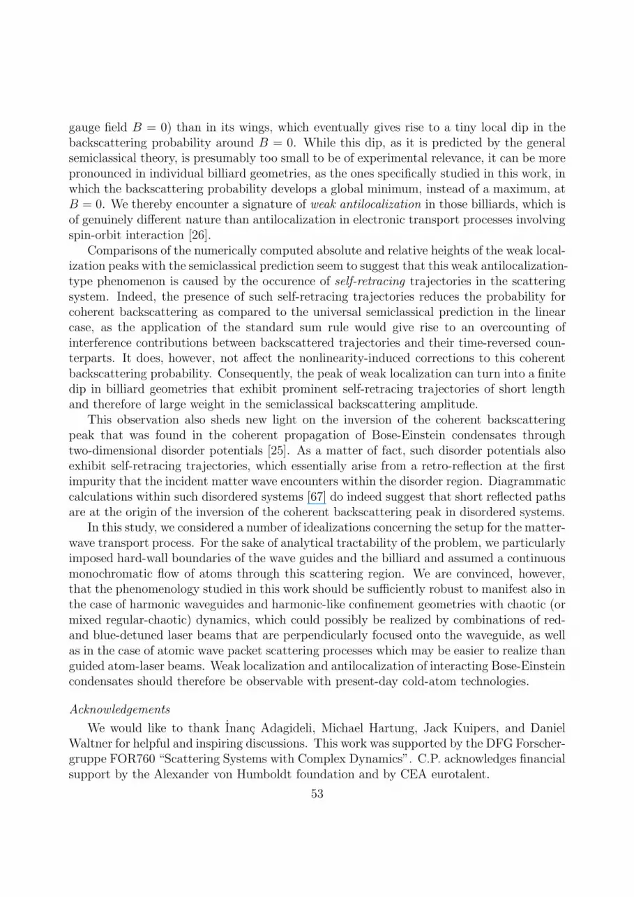
gauge field B = 0) than in its wings, which eventually gives rise to a tiny local dip in thebackscattering probability around B = 0. While this dip, as it is predicted by the generalsemiclassical theory, is presumably too small to be of experimental relevance, it can be morepronounced in individual billiard geometries, as the ones specifically studied in this work, inwhich the backscattering probability develops a global minimum, instead of a maximum, atB = 0. We thereby encounter a signature of weak antilocalization in those billiards, which isof genuinely different nature than antilocalization in electronic transport processes involvingspin-orbit interaction [26].

Comparisons of the numerically computed absolute and relative heights of the weak local-ization peaks with the semiclassical prediction seem to suggest that this weak antilocalization-type phenomenon is caused by the occurence of self-retracing trajectories in the scatteringsystem. Indeed, the presence of such self-retracing trajectories reduces the probability forcoherent backscattering as compared to the universal semiclassical prediction in the linearcase, as the application of the standard sum rule would give rise to an overcounting ofinterference contributions between backscattered trajectories and their time-reversed coun-terparts. It does, however, not affect the nonlinearity-induced corrections to this coherentbackscattering probability. Consequently, the peak of weak localization can turn into a finitedip in billiard geometries that exhibit prominent self-retracing trajectories of short lengthand therefore of large weight in the semiclassical backscattering amplitude.

This observation also sheds new light on the inversion of the coherent backscatteringpeak that was found in the coherent propagation of Bose-Einstein condensates throughtwo-dimensional disorder potentials [25]. As a matter of fact, such disorder potentials alsoexhibit self-retracing trajectories, which essentially arise from a retro-reflection at the firstimpurity that the incident matter wave encounters within the disorder region. Diagrammaticcalculations within such disordered systems [67] do indeed suggest that short reflected pathsare at the origin of the inversion of the coherent backscattering peak in disordered systems.

In this study, we considered a number of idealizations concerning the setup for the matter-wave transport process. For the sake of analytical tractability of the problem, we particularlyimposed hard-wall boundaries of the wave guides and the billiard and assumed a continuousmonochromatic flow of atoms through this scattering region. We are convinced, however,that the phenomenology studied in this work should be sufficiently robust to manifest also inthe case of harmonic waveguides and harmonic-like confinement geometries with chaotic (ormixed regular-chaotic) dynamics, which could possibly be realized by combinations of red-and blue-detuned laser beams that are perpendicularly focused onto the waveguide, as wellas in the case of atomic wave packet scattering processes which may be easier to realize thanguided atom-laser beams. Weak localization and antilocalization of interacting Bose-Einsteincondensates should therefore be observable with present-day cold-atom technologies.

Acknowledgements

We would like to thank Inanc Adagideli, Michael Hartung, Jack Kuipers, and DanielWaltner for helpful and inspiring discussions. This work was supported by the DFG Forscher-gruppe FOR760 “Scattering Systems with Complex Dynamics”. C.P. acknowledges financialsupport by the Alexander von Humboldt foundation and by CEA eurotalent.

53

Appendix A. Numerical computation of stationary scattering states

In this appendix, we explain how we numerically compute stationary solutions ψ ≡ψ(r) of the time-dependent inhomogeneous Gross-Pitaevskii equation (5). Such stationarysolutions satisfy the nonlinear equation

[µ−H ]ψ(r)− g(r)~2

2m|ψ(r)|2ψ(r)− S(r) = 0 (A.1)

with S(r) = S0χi(y)δ(x− xL), which is equivalent to Eq. (62). This equation is discretizedon a two-dimensional lattice where only points inside the cavity and the leads are taken intoaccount. The single-particle Hamiltonian H given by Eq. (6) can be approximated using afinite-difference scheme [63] where we incorporate the vector potential using a Peierls phase[68]. We choose the lattice spacing ∆ small enough that the approximation error [whichscales as O(∆2)] becomes negligible, which is the case for roughly 30 lattice points perwavelength. The interaction strength g(r) is, as explained in Ref. [69], considered to beconstant within the scattering region and adiabatically ramped off in the leads [70]. Theeffects of the infinite leads can then be incorporated through self-energies as in the recursiveGreen function method [64, 71], which allows one to restrict the numerical computation toa finite spatial region.

The complex solution ψ(r) of the nonlinear wave equation (A.1) can be represented as a2N -dimensional real vector where N is the number of grid points. Defining

F : R2N −→ R2N , ψ(r) 7−→ [µ−H0]ψ(r)− g(r)

~2

2m|ψ(r)|2ψ(r)− S(r) , (A.2)

we search now for a solution of F (ψ) = 0. This is done with Newton’s method [72]. Oneselects a starting vector ψ0(r) and constructs a sequence of vectors ψk∞k=1 (here k is theiteration number) using the iteration ψk+1 = ψk − (DF )−1 F (ψk). If the derivate DF atthe solution is not singular, this iteration is guaranteed to converge to a solution of thenonlinear equation (A.1), provided the starting vector is chosen in a suitably close vicinityof this solution.

The efficiency of this method strongly depends on the starting vector ψ0(r). An obviouschoice would be the solution of the linear wave equation (for g = 0). This choice, however,works out only for very small nonlinearities. In the general case, one has to use a continuationmethod [72, 73]. To this end, we consider g, i.e. the constant value of the interaction strengthwithin the billiard [74], as an additional free parameter and reinterpret F ≡ F [ψ(r); g] as afunction F : R

2N×R → R2N . Now F−1(0) is a one-dimensional manifold [75] which can be

conveniently parametrized by the arclength s through the parametric curve s 7→ [g(s), ψ(s)].Starting from g = 0, the numerical algorithm follows this curve until the desired value g ofthe nonlinearity strength is reached, and returns the wavefunction ψ(r) that is obtained atthe end of this curve-tracking process [76].

Fig. A.16 shows, for a specific set of parameters, a projection of this curve onto the two-dimensional parameter space spanned by the nonlinearity strength g and the total trans-mission that is associated with the stationary scattering state ψ(r). As is characteristic for

54

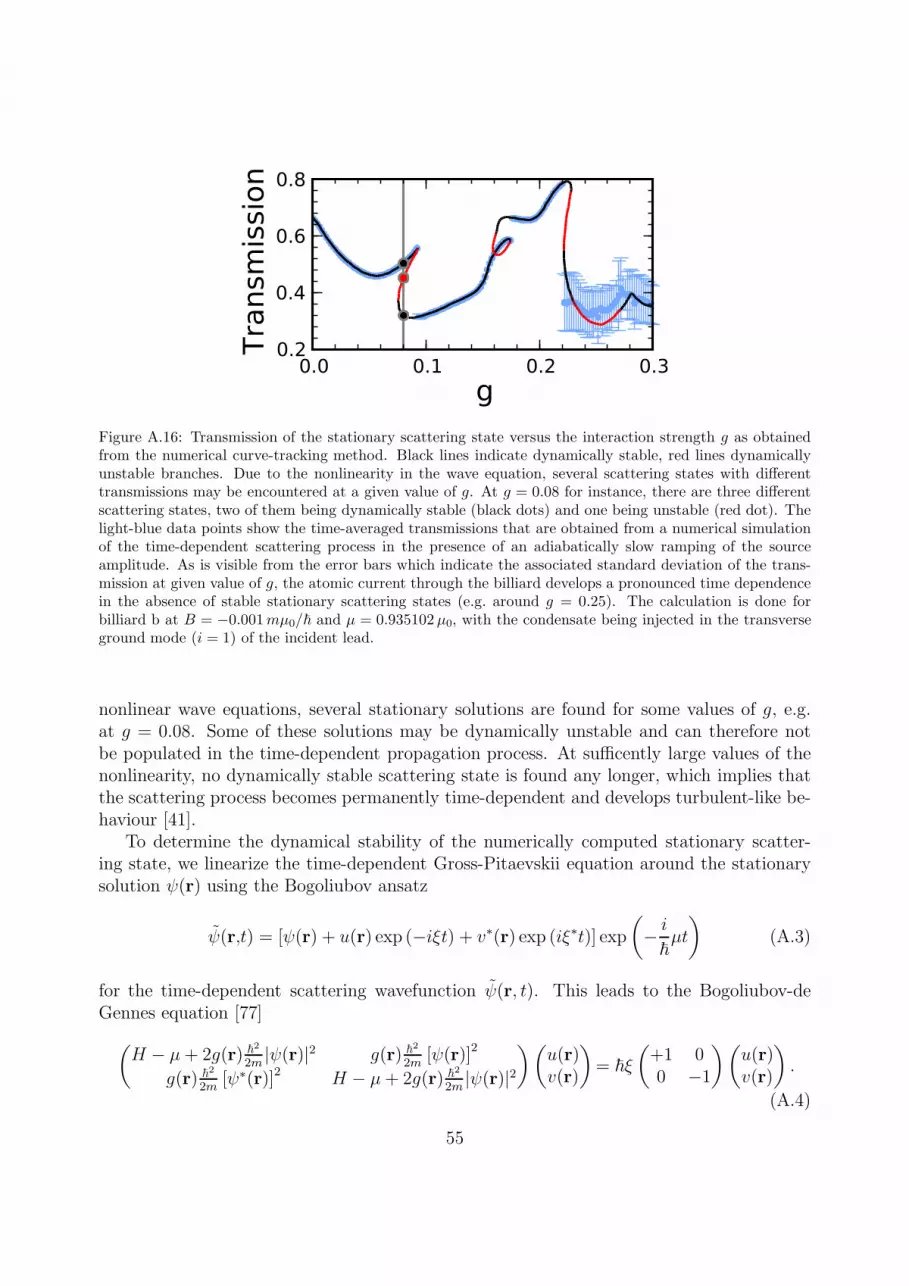
0.0 0.1 0.2 0.3

g

0.2

0.4

0.6

0.8

Transm

ission

Figure A.16: Transmission of the stationary scattering state versus the interaction strength g as obtainedfrom the numerical curve-tracking method. Black lines indicate dynamically stable, red lines dynamicallyunstable branches. Due to the nonlinearity in the wave equation, several scattering states with differenttransmissions may be encountered at a given value of g. At g = 0.08 for instance, there are three differentscattering states, two of them being dynamically stable (black dots) and one being unstable (red dot). Thelight-blue data points show the time-averaged transmissions that are obtained from a numerical simulationof the time-dependent scattering process in the presence of an adiabatically slow ramping of the sourceamplitude. As is visible from the error bars which indicate the associated standard deviation of the trans-mission at given value of g, the atomic current through the billiard develops a pronounced time dependencein the absence of stable stationary scattering states (e.g. around g = 0.25). The calculation is done forbilliard b at B = −0.001mµ0/~ and µ = 0.935102µ0, with the condensate being injected in the transverseground mode (i = 1) of the incident lead.

nonlinear wave equations, several stationary solutions are found for some values of g, e.g.at g = 0.08. Some of these solutions may be dynamically unstable and can therefore notbe populated in the time-dependent propagation process. At sufficently large values of thenonlinearity, no dynamically stable scattering state is found any longer, which implies thatthe scattering process becomes permanently time-dependent and develops turbulent-like be-haviour [41].

To determine the dynamical stability of the numerically computed stationary scatter-ing state, we linearize the time-dependent Gross-Pitaevskii equation around the stationarysolution ψ(r) using the Bogoliubov ansatz

ψ(r,t) = [ψ(r) + u(r) exp (−iξt) + v∗(r) exp (iξ∗t)] exp

(− i

~µt

)(A.3)

for the time-dependent scattering wavefunction ψ(r, t). This leads to the Bogoliubov-deGennes equation [77]

(H − µ+ 2g(r) ~

2

2m|ψ(r)|2 g(r) ~

2

2m[ψ(r)]2

g(r) ~2

2m[ψ∗(r)]2 H − µ+ 2g(r) ~

2

2m|ψ(r)|2

)(u(r)v(r)

)= ~ξ

(+1 00 −1

)(u(r)v(r)

).

(A.4)

55

0.00 0.05 0.10

g

0.00

0.05

0.10

0.15

0.20

fract

ion

more than one stableonly unstable

Figure A.17: This figure shows as a function of g the fraction of configurations of B, µ and the incident modei that exhibit only dynamically unstable solutions (red curve) or support more than one dynamically stablesolution (blue curve). In the latter case, we select the one that is first encountered in the curve-trackingalgorithm starting from g = 0.

This generalized eigenvalue problem is numerically solved using the implicit restartedArnoldi method as realized in the software library ARPACK [78]. Special care must be takenin order to describe the infinite leads properly. This is done using the method of smoothexterior complex scaling [79] which exponentially damps the outgoing waves of the collectivemodes in the leads. As a consequence, the Bogoliubov eigenfrequencies ξ become complex.If one of them is found to exhibit a positive imaginary part, i.e. Im(ξ) > 0, we can inferfrom Eq. (A.3) that the scattering state ψ(r) under consideration is dynamically unstable.

Fig. A.17 shows (red curve) the fraction of parameter configurations of the chemical po-tential µ, the magnetic field B, and the incident mode number i for which no dynamicallystable scattering state is found. This fraction of unstable configurations is found to increasewith the nonlinearity strength g, which imposes restrictions on the shape of the cavities andthe maximum value of g one can use for numerical simulations. In particular, we find thatthe fraction of configurations that support no stable solution increases rather rapidly with gfor small widths of the leads, i.e. for a very low number of open channels. This is attributedto the reduced spectral width that quasi-bound resonance states within the billiard exhibitin that case, which in turn leads to an enhanced interaction energy

∫drg(r)|ψ(r)|4 at such

resonances. Rather wide leads with a large number of open channels, on the other hand,compromise the effect of weak localization and reduce the visibility of its signature in thereflection and transmission probabilities. For the billiard sizes and geometries under con-sideration, the fraction of configurations with unstable solutions remains below 0.02 untilg = 0.08.

When encountering a configuration with only unstable solutions, we select the one thatexhibits the smallest Lyapunov exponent, the latter being defined by the largest imaginarypart of the eigenvalues ξ of the Bogoliubov-de Gennes equations (A.4). This choice is sup-ported by time-dependent propagations of the inhomogeneous Gross-Pitaevskii equation (5),which directly simulate, as in Ref. [25], the time-dependent scattering process in the presenceof an adiabatic increase of the source amplitude. In such simulations, which were carried out

56

for specific parameter configurations, we find, for not too large values of g, that the time-dependent current in the transmitted lead displays regular oscillations around the currentof the stationary solution that is the least unstable one and exhibits the smallest Lyapunovexponent. The time-averaged transmission, which is the main experimental observable insuch scattering processes, is then correctly reproduced by the transmission of the unstablestationary scattering state. For larger values of g, however, the time-dependent dynam-ics of the propagating wavefunction becomes chaotic, which means that the transmissionassociated with an unstable stationary scattering state loses its significance.

Appendix B. The eikonal approximation

In this appendix, we explicitly derive the semiclassical expression for the Green functionin the presence of a weak perturbation of the Hamiltonian. Considering the HamiltonianH = H0 + δH with H0 ≡ H0(p, r) the unperturbed part and δH ≡ δH(p, r) a perturbationthat is slowly varying with r, and defining G0 ≡ (E −H0 + i0)−1, we can express the Greenfunction of the system by means of a Dyson equation of the form

G ≡ (E −H + i0)−1 = G0 +G0δHG = G0

∞∑

k=0

(δHG0)k . (B.1)

Let us first evaluate the first-order term of this Born series,

δG(1)(r, r′, E) ≡ 〈r|G0δHG0|r′〉 =∫d2r′′G0(r, r

′′, E)δH(p, r′′)G0(r′′, r′, E) , (B.2)

in the semiclassical approximation. Using the semiclassical expression (10) for the Greenfunction,

G0(r, r′, E) =

∑

γ

Aγ(r, r′, E)exp

[i

~Sγ(r, r

′, E)− iπ

2µγ

]. (B.3)

we see that the momentum operator p in δH acts, in leading semiclassical order (i.e., inlowest order in ~), only on the action integrals Sγ(r

′′, r′, E) in the exponents. This meansthat p can be replaced by the final momenta of the trajectories leading from r′ to r′′. Wetherefore obtain

δG(1)(r, r′, E) =

∫d2r′′

∑

γ1,γ2

Aγ2(r, r′′, E)Aγ1(r

′′, r′, E)δH(p′′, r′′)

× exp

i

~[Sγ2(r, r

′′, E) + Sγ1(r′′, r′, E)]−iπ

2(µγ1 + µγ2)

(B.4)

with p′′ ≡ pfγ1(r

′′, r′, E), where the indices γ1 and γ2 respectively represent the trajectoriesfrom r′ to r′′ and from r′′ to r.

57

Using now the fact that Aγ1 , Aγ2 , and δH(p′′, r′′) are slowly varying functions of r′′ onthe length scale of the de Broglie wavelength of the atoms, we can apply the stationaryphase approximation to evaluate the integral over r′′. The stationary phase condition yields

∂

∂r′′[Sγ2(r, r

′′, E) + Sγ1(r′′, r′, E)] = 0 , (B.5)

i.e., pfγ1(r′′, r′, E) = pi

γ2(r, r′′, E). This condition is satisfied if and only if the trajectory γ2

is the direct continuation of γ1. The double sum in Eq. (B.4) can therefore be contractedto a single sum over trajectories γ that are going from r′ to r at energy E. Combining theprefactors that result from the spatial integration perpendicular to this trajectory as wellas from the amplitudes Aγ1 , Aγ2 , and transforming the spatial integration parallel to thetrajectory into an integration along the propagation time, we finally obtain

δG(1)(r, r′, E) = − i

~

∑

γ

Aγ(r, r′, E)exp

[i

~Sγ(r, r

′, E)− iπ

2µγ

] ∫ Tγ

0

δH [pγ(t),qγ(t)]dt .

(B.6)Similarly, higher order terms in the Born series (B.1) can be evaluated yielding

δG(k)(r, r′, E) ≡ 〈r|G0(δHG0)k|r′〉

=∑

γ

Aγ(r, r′, E)exp

[i

~Sγ(r, r

′, E)− iπ

2µγ

]

× 1

k!

(− i

~

∫ Tγ

0

δH [pγ(t),qγ(t)]dt

)k

. (B.7)

This finally yields the modified Green function

G(r, r′, E) =∑

γ

Aγ(r, r′, E)exp

[i

~Sγ(r, r

′, E)− iπ

2µγ −

i

~φγ(r, r

′, E)

](B.8)

where

φγ(r, r′, E) ≡

∫ Tγ

0

δH [pγ(t),qγ(t)]dt . (B.9)

represents an effective modification of the action integral Sγ due to the presence of theperturbation. Eq. (B.8) reflects a general result in classical mechanics that, to leading orderin the perturbation, the action difference between unperturbed and perturbed orbits is, forperiodic orbits, given by Eq. (B.9) [80].

In the case of a perturbation due to a weak magnetic field, we have

δH(p, r) = − 1

mA(r) · p+

1

2mA2(r) . (B.10)

Hence, we can write φγ = −ϕγ − ϕγ with

ϕγ(r, r′, E) ≡ 1

m

∫ Tγ

0

pγ(t) ·A[qγ(t)]dt , (B.11)

ϕγ(r, r′, E) ≡ − 1

2m

∫ Tγ

0

A2[qγ(t)]dt (B.12)

58

corresponding, respectively, to a paramagnetic and a diamagnetic contribution to the effec-tive action integral.

Also the presence of a weak nonlinearity within the scattering system can be accountedfor in this framework, provided only ladder contributions are considered. Comparing Eq. (66)in the cases (68) and (68) with Eq. (B.2), we see that we have to set

δH(r) = 2g~2

2m|ψ(0)(r)|2d (B.13)

where |ψ(0)(r)|2d represents, according to Eq. (72), the density at position r as evaluatedwithin the diagonal approximation. We then obtain the effective modification of the actionintegral [defined by χγ(r, r

′, µ) in Sec. 3.3] as

φγ(r, r′, µ) = g

~2

m

∫ Tγ

0

|ψ(0)[qγ(t)]|2d dt . (B.14)

Appendix C. Sum rules

In this appendix, we derive the generalized Hannay-Ozorio de Almeida sum rules [46, 47]that we need in order to evaluate energy averages of squares of the Green function in thediagonal approximation. To keep the derivation as general as possible, we introduce a newparametrization of the initial and final phase space points according to (p, r) ≡ (ξ1, ξ2, ξ3, ξ4)and (p′, r′) ≡ (η′1, η

′2, η

′3, η

′4) where the sets (ξ1, ξ2, ξ3, ξ4) and (η′1, η2,

′ η3,′ η′4) contain the com-

ponents (px, py, x, y) and (p′x, p′y, x

′, y′) of the final and initial phase space points, respectively,in some arbitrary order. We shall now be interested in the Green function from the coordi-nates (η′1, η

′2) to the coordinates (ξ1, ξ2). In the diagonal approximation, the energy average

of the modulus square of this Green function reads⟨|G [(ξ1, ξ2), (η

′1, η

′2), E]|2

⟩d

=∑

γ

⟨|Aγ [(ξ1, ξ2), (η

′1, η

′2), E]|2

⟩(C.1)

=1

2π~3

∑

γ

⟨∣∣∣∣∣det∂[(p′x, p

′y), (x

′, y′), T]

∂ [(ξ1, ξ2), (η′1, η

′2), E]

∣∣∣∣∣

⟩. (C.2)

We furthermore need the corresponding expression for the crossed average which includes,in addition, a magnetic dephasing. This yields

〈G∗ [(η′1, η′2), (ξ1, ξ2), E]G [(ξ1, ξ2), (η

′1, η

′2), E]〉c =

=∑

γ

⟨|Aγ [(ξ1, ξ2), (η

′1, η

′2), E]|2

⟩exp

(−TγτB

)(C.3)

=1

2π~3

∑

γ

⟨∣∣∣∣∣det∂[(p′x, p

′y), (x

′, y′), T]

∂ [(ξ1, ξ2), (η′1, η′2), E]

∣∣∣∣∣

⟩exp

(−TγτB

)(C.4)

where τB ∼ B−2 [see Eq. (53)] is the dephasing time.

59

Applying standard rules for multidimensional integrations over δ-distributions, we canderive

∑

γ

∣∣∣∣det∂[(p′x, p

′y), (x

′, y′), T ]

∂[(ξ1, ξ2), (η′1, η′2), E]

∣∣∣∣ f(Tγ) =

∫dξ3

∫dξ4

∫dη′3

∫dη′4

∫ ∞

0

dTδ [E −H0(p′, r′)]

×δ [r− q(p′, r′, T )] δ [p− p(p′, r′, T )] f(T ) (C.5)

for any f(T ), where we define q(p′, r′, T ) ≡ (qx, qy)(p′, r′, T ) and p(p′, r′, T ) ≡ (px, py)(p

′, r′, T )as the position and momentum variables that result from the propagation of a classical trajec-tory over time T with the initial values p′ ≡ (p′x, p

′y) and r′ ≡ (x′, y′). Furthermore, assuming

classical ergodicity, which is valid if the dynamics within the billiard is fully chaotic, we canstate that each phase-space point (p, r) within the billiard has equal probability to be hit bya given trajectory after a given evolution time T , provided it lies within the shell of constantenergy E. This probability, however, decreases exponentially with the evolution time, dueto the possibility for escape from the billiard via the openings. We therefore obtain

〈δ [r− q(p′, r′, T )] δ [p− p(p′, r′, T )]〉 = δ [H0(p′, r′)−H0(p, r)]∫

d2p∫d2qδ [H0(p′, r′)−H0(p,q)]

exp

(− T

τD

)

(C.6)where the “dwell time” τD corresponds to the mean evolution time that a classical trajectoryspends within the billiard before escaping to one of the waveguides. This altogether yields

⟨|G [(ξ1, ξ2), (η

′1, η

′2), E]|2

⟩d=

τD2π~3

∫dξ3∫dξ4δ [E −H0(p, r)]

∫dη′3∫dη′4δ [E −H0(p

′, r′)]∫d2p∫d2qδ [E −H0(p,q)]

(C.7)and

〈G∗ [(η′1, η′2), (ξ1, ξ2), E]G [(ξ1, ξ2), (η

′1, η

′2), E]〉c =

1

1 + τD/τB

⟨|G [(ξ1, ξ2), (η

′1, η

′2), E]|2

⟩

d.

(C.8)The phase space integrals appearing in Eq. (C.7) can be straightforwardly computed.

We obtain∫d2qδ [E −H0(p,q)] = Ωδ

(E − p2

2m

), (C.9)

∫d2pδ [E −H0(p,q)] = 2πmχΩ(q) , (C.10)

∫d2p

∫d2qδ [E −H0(p,q)] = 2πmΩ , (C.11)

where χΩ(q) represents the characteristic function of the scattering system and Ω denotesthe area of the billiard. Furthermore, for the case of “mixed” initial or final conditionsz ≡ (xL, py) specified within the incident lead, we calculate

∫dy

∫dpxδ [E −H0(p,q)] =

∫ W

0

dy

∫ ∞

0

dpxδ

(E − p2x + p2y

2

)=

mW√2mE − p2y

. (C.12)

60

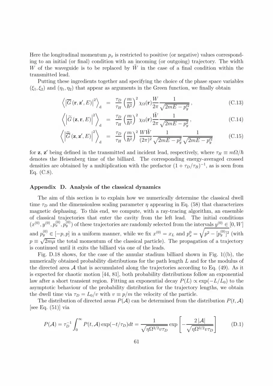
Here the longitudinal momentum px is restricted to positive (or negative) values correspond-ing to an initial (or final) condition with an incoming (or outgoing) trajectory. The widthW of the waveguide is to be replaced by W in the case of a final condition within thetransmitted lead.

Putting these ingredients together and specifying the choice of the phase space variables(ξ1, ξ2) and (η1, η2) that appear as arguments in the Green function, we finally obtain

⟨∣∣G (r, z′, E)∣∣2⟩

d=

τDτH

(m~2

)2χΩ(r)

W

2π

1√2mE − p′2y

, (C.13)

⟨∣∣∣G (z, r, E)∣∣∣2⟩

d

=τDτH

(m~2

)2χΩ(r)

W

2π

1√2mE − p2y

, (C.14)

⟨∣∣∣G (z, z′, E)∣∣∣2⟩

d

=τDτH

(m~2

)2 WW

(2π)21√

2mE − p2y

1√2mE − p′2y

(C.15)

for z, z′ being defined in the transmitted and incident lead, respectively, where τH ≡ mΩ/~denotes the Heisenberg time of the billiard. The corresponding energy-averaged crosseddensities are obtained by a multiplication with the prefactor (1 + τD/τB)

−1, as is seen fromEq. (C.8).

Appendix D. Analysis of the classical dynamics

The aim of this section is to explain how we numerically determine the classical dwelltime τD and the dimensionless scaling parameter η appearing in Eq. (58) that characterizesmagnetic dephasing. To this end, we compute, with a ray-tracing algorithm, an ensembleof classical trajectories that enter the cavity from the left lead. The initial conditions(x(0), y(0), p

(0)x , p

(0)y ) of these trajectories are randomly selected from the intervals y(0) ∈ [0,W ]

and p(0)y ∈ [−p, p] in a uniform manner, while we fix x(0) = xL and p0x =

√p2 − [p

(0)y ]2 (with

p ≡ √2mµ the total momentum of the classical particle). The propagation of a trajectory

is continued until it exits the billiard via one of the leads.Fig. D.18 shows, for the case of the annular stadium billiard shown in Fig. 1((b), the

numerically obtained probability distributions for the path length L and for the modulus ofthe directed area A that is accumulated along the trajectories according to Eq. (49). As itis expected for chaotic motion [44, 81], both probability distributions follow an exponentiallaw after a short transient region. Fitting an exponential decay P (L) ∝ exp(−L/L0) to theasymptotic behaviour of the probability distribution for the trajectory lengths, we obtainthe dwell time via τD = L0/v with v ≡ p/m the velocity of the particle.

The distribution of directed areas P (A) can be determined from the distribution P (t,A)[see Eq. (51)] via

P (A) = τ−1D

∫ ∞

0

P (t,A) exp(−t/τD)dt =1√

ηΩ3/2vτDexp

[− 2 |A|√

ηΩ3/2vτD

](D.1)

61

0 10 20 30 40 50 60

L/Ω12

12

8

4

0

logP(L

)

histogramexponential fit

0 1 2 3 4

A/Ω

8

4

0

logP(A

)

histogramexponential fit

Figure D.18: Probability distributions (blue lines) for the path length L (left panel) and for the directedarea A (right panel) for the case of the the annular stadium billiard shown in Fig. 1((b). Neglecting a shorttransient region, an exponential decay (red dashed lines) is fitted to these distributions.

and is also predicted to decrease exponentially with |A| [44, 81]. The exponential decayP (A) ∝ exp (−|A|/A0) that is numerically encountered after a short transient region allowsus to determine the characteristic scaling parameter via η = 4A2

0/(Ω3/2vτD), using the dwell

time τD that is obtained from the length distribution as explained above.Comparing the numerically computed dwell time τ

(num.)D with the “universal” prediction

(43), we obtain τ(num.)D ≃ 0.79(πΩ)/[(W + W )v]. This deviation is attributed to the finite

width of the leads, which effectively compromises the assumption of ergodic motion thatunderlies the derivation of Eq. (43). Regular islands of appreciable size, which might alsogive rise to a deviation of the dwell time from the universal prediction, could not be identifiedin the phase space of the two billiards.

Appendix E. Frequent integrals in the calculations of loop corrections

Appendix E.1. The standard encounter integral

In this appendix, we calculate the contribution of the encounter region. We first considerthe absence of a nonlinearity. The corresponding integral is given by

In1 (E) =

⟨∫ c

−c

ds

∫ c

−c

du1

Σ(E)tenc(su)exp

(i

~su

)exp

(−tenc(su)

τn

)⟩, (E.1)

where 1/τn≡1/τD + n/τB accounts for the fact that we can have n ∈ 0, 1, 2 stretches witha gauge field dependence within the encounter region, and Σ(E) = 2πmΩ is the volume ofthe energy shell in phase space. Following Ref. [58], we first split the integration over u intwo parts, ∫ c

−c

du . . . =

∫ 0

−c

du . . .+

∫ c

0

du . . . , (E.2)

and make the variable transformation (s, u) 7→ (S, y) with S ≡ su/c2 ∈ [−1, 1] andy ≡ c/|u| = ∓c/u ∈ [1, 1/S], with the associated Jacobian determinant c2/y, where thesign in the definition of y refers to the first and the second integral on the right-hand side of

62

Eq. (E.2), respectively. In physical terms, we transform here from the phase space coordi-nates s, u to the action difference su measured in terms of c2, and to a coordinate y relatedto the time tu = (1/λ) ln(c/u) needed for the unstable phase space coordinate to evolve fromthe Poincare surface of section P to the limiting value ∓c.

As tenc(su) = (1/λ) ln(c2/|su|) = tenc(|S|) does not depend on y, we obtain

∫ 1/|S|

1

dy1

y= ln

(1

|S|

)= λtenc(|S|) (E.3)

for the integration over y. We then have

In1 (E) =

⟨2c2λ

Σ(E)

∫ 1

−1

dS exp

(i

~Sc2)exp

(−tenc(|S|)

τn

)⟩

=

⟨4c2λ

Σ(E)

∫ 1

0

dS cos

(Sc2

~

)S1/(λτn)

⟩

=

⟨4~λ

Σ(E)sin

(c2

~

)⟩−⟨

4~

Σ(E)τn

∫ 1

0

dSsin(Sc2/~)

SS1/(λτn)

⟩. (E.4)

As the limiting scale c for the coordinates s and u (i.e., the scale until which the linerizationaround the reference trajectory is still valid) generally depends on the energy E, the first termin Eq. (E.4) is expected to strongly oscillate when varying E and would thus vanish whenperforming the energy average. For the second term, we obtain after the transformationS 7→ S ′ ≡ Sc2/~

In1 (E) = −⟨

4~

Σ(E)τn

∫ c2/~

0

dS ′ sin (S′)

S ′

(S ′~

c2

)1/(λτn)⟩. (E.5)

Assuming that the Ehrenfest time τE ≡ (1/λ) ln(c2/~) is much smaller than the dwell timeτD and the magnetic dephasing time scale τB, we have τE ≪ τn as well as λτn ≫ 1 and canapproximate (

S ′~

c2

)1/(λτn)

= (S ′)1/(λτn) exp

[−τEτn

]≃ 1 . (E.6)

The remaining integral can then be evaluated in the semiclassical limit ~ → 0 by sendingthe upper limit of the integration (E.5) to infinity, which finally yields

In1 (E) = − 4~

Σ(E)τn

∫ ∞

0

dSsin (S)

S= − 2π~

Σ(E)τn= − 1

τDτH

(1 + n

τDτB

). (E.7)

Appendix E.2. The encounter integral with an embedded nonlinearity event

Now we consider the presence of a nonlinearity event within the encounter region. Wefirst focus on the case that the nonlinearity event is moving along a stretch all the way

63

Figure E.19: Sketch of the two different possibilities for a nonlinearity event to enter the encounter region. Inthe scenario depicted on the left-hand side, the nonlinearity event moves along a stretch all the way throughthe encounter region. On the right-hand side, two of the four encounter stretches end at the nonlinearityblock. This gives rise to a reduced encounter duration tenc(t, u) = t+ tu which depends on the time intervalt between the nonlinearity event and the Poincare surface of section P , and on the time tu = (1/λ) ln(c/|u|)between P and the borders of the encounter region.

through the encounter region, as depicted on the left-hand side of Fig. E.19. For this case,we have to evaluate the integral

I2(E) =

⟨ c∫

−c

c∫

−c

dsdu1

Σ(E)tenc(su)exp

(i

~su

)exp

[−tenc(su)

τD

] ∫ tenc(su)

0

dt exp

(− t

τB

)⟩,

(E.8)where the additional integration variable t represents the location of the nonlinearity ona stretch within the encounter region. The gauge field dependence, manifested by thedephasing factor exp(−t/τB), emerges from the stretch along which the nonlinearity moves.We have ∫ tenc

0

dt exp

(− t

τB

)= τB

[1− exp

(−tencτB

)], (E.9)

which would also be obtained if the integrand in Eq. (E.8) was exp[− (tenc − t) /τB], corre-sponding to the case that the other part of the stretch guiding the nonlinearity event wouldprovide the gauge field dependence. Using the results from section Appendix E.1, we obtain

I2(E) = τB[I01 (E)− I11 (E)

]=

1

τH. (E.10)

We now analyze the second scenario, shown on the right-hand side of Fig. E.19, wherestretches of the encounter region terminate at a nonlinearity. The integral that has to beevaluated in this case is given by

In3 (E) =

⟨ c∫

−c

c∫

−c

dsdu

∫ (1/λ) ln(c/|s|)

0

dt1

Σ(E)tenc(t, u)exp

(i

~su

)exp

(− tenc(t, u)

τn

)⟩,

(E.11)where we define tenc(t, u)≡t + (1/λ) ln(c/|u|) as the reduced encounter time and 1/τn ≡1/τD +n/τB, with n = 0, 1, 2 the number of pairs of imbalanced stretches that give rise to a

64

gauge field dependence. As indicated in Fig. E.19, the integration variable t represents thetime between the nonlinearity and the Poincare surface of section P within which the stableand unstable coordinates are defined.

Following Refs. [58, 59, 60], we split, as in Section Appendix E.1, the integration overu according to Eq. (E.2) and make the variable transformation (s, u, t) 7→ (S, y, t) withS ≡ su/c2 ∈ [−1, 1], t ≡ tenc(t, u) = t+(1/λ) ln(c/|u|) ∈ [0, (1/λ) ln(1/|S|)], and y ≡ c/|u| ∈[1, exp(λt)], with the associated Jacobian determinant c2/y. The integration over y yields

∫ exp(λt)

1

dy1

y= λt . (E.12)

We then evaluate

In3 (E) =

⟨2c2λ

Σ(E)

∫ 1

−1

dS

∫ (1/λ) ln(1/|S|)

0

dt exp

(i

~Sc2)exp

(− t

τn

)⟩

=

⟨2c2λτnΣ(E)

∫ 1

−1

dS[1− |S|1/(τnλ)

]exp

(i

~Sc2)⟩

=

⟨4c2λτnΣ(E)

[~

c2sin

(c2

~

)−∫ 1

0

dS cos

(Sc2

~

)S1/(τnλ)

]⟩. (E.13)

The first contribution in the last line of Eq. (E.13) vanishes when performing the energyaverage, whereas the second term yields [−(~π)/(2λc2τn)], as seen in Section Appendix E.1.We thus obtain

In3 (E) =4c2λτnΣ(E)

~π

2λc2τn=

2π~

Σ(E)=

1

τH. (E.14)

References

References

[1] R. Dumke, T. Muther, M. Volk, W. Ertmer, G. Birkl, Phys. Rev. Lett. 89 (2002) 220402.[2] R. Folman, P. Kruger, D. Cassettari, B. Hessmo, T. Maier, J. Schmiedmayer, Phys. Rev. Lett. 84

(2000) 4749.[3] J. Fortagh, C. Zimmermann, Rev. Mod. Phys. 79 (2007) 235.[4] W. Guerin, J.-F. Riou, J. P. Gaebler, V. Josse, P. Bouyer, A. Aspect, Phys. Rev. Lett. 97 (2006)

200402.[5] A. Couvert, M. Jeppesen, T. Kawalec, G. Reinaudi, R. Mathevet, D. Guery-Odelin, EPL 83 (2008)

50001.[6] V. Milner, J. L. Hanssen, W. C. Campbell, M. G. Raizen, Phys. Rev. Lett. 86 (2001) 1514.[7] N. Friedman, A. Kaplan, D. Carasso, N. Davidson, Phys. Rev. Lett. 86 (2001) 1518.[8] K. Henderson, C. Ryu, C. MacCormick, M. G. Boshier, New J. Phys. 11 (2009) 043030.[9] J. Billy, V. Josse, Z. Zuo, A. Bernard, B. Hambrecht, P. Lugan, D. Clement, L. Sanchez-Palencia,

P. Bouyer, A. Aspect, Nature 453 (2008) 891.[10] G. Roati, C. D’Errico, L. Fallani, M. Fattori, C. Fort, M. Zaccanti, G. Modugno, M. Modugno, M. In-

guscio, Nature 453 (2008) 895.[11] A. Stibor, S. Kraft, T. Campey, D. Komma, A. Gunther, J. Fortagh, C. J. Vale, H. Rubinsztein-Dunlop,

C. Zimmermann, Phys. Rev. A 76 (2007) 033614.

65

[12] Y.-J. Lin, R. L. Compton, A. R. Perry, W. D. Phillips, J. V. Porto, I. B. Spielman, Phys. Rev. Lett.102 (2009) 130401.

[13] G. Juzeliunas, P. Ohberg, J. Ruseckas, A. Klein, Phys. Rev. A 71 (2005) 053614.[14] J. Ruseckas, G. Juzeliunas, P. Ohberg, M. Fleischhauer, Phys. Rev. Lett. 95 (2005) 010404.[15] J. Dalibard, F. Gerbier, G. Juzeliunas, P. Ohberg, Rev. Mod. Phys. 83, 1523 (2011) 83 (2011) 1523.[16] B. L. Altshuler, D. Khmel’nitzkii, A. I. Larkin, P. A. Lee, Phys. Rev. B 22 (1980) 5142.[17] G. Bergmann, Phys. Rep. 107 (1984) 1.[18] M. P. Van Albada, A. Lagendijk, Phys. Rev. Lett. 55 (1985) 2692.[19] P.-E. Wolf, G. Maret, Phys. Rev. Lett. 55 (1985) 2696.[20] A. G. Aronov, Y. V. Sharvin, Rev. Mod. Phys. 59 (1987) 755.[21] A. M. Chang, H. U. Baranger, L. N. Pfeiffer, K. W. West, Phys. Rev. Lett. 73 (1994) 2111.[22] B. L. Altshuler, A. G. Aronov, D. E. Khmelnitsky, J. Phys. C: Solid State Phys. 15 (1982) 7367.[23] B. L. Altshuler, A. G. Aronov, in: A. L. Efros, M. Pollak (Eds.), Electron-electron interaction in

disordered systems, Elsevier, Amsterdam, 1985, p. 1.[24] R. S. Whitney, P. Jacquod, C. Petitjean, Phys. Rev. B 77 (2008) 045315.[25] M. Hartung, T. Wellens, C. A. Muller, K. Richter, P. Schlagheck, Phys. Rev. Lett. 101 (2008) 020603.[26] D. M. Zumbuhl, J. B. Miller, C. M. Marcus, K. Campman, A. C. Gossard, Phys. Rev. Lett. 89 (2002)

276803.[27] H. U. Baranger, R. A. Jalabert, A. D. Stone, Chaos 3 (1993) 665.[28] K. Richter, M. Sieber, Phys. Rev. Lett. 89 (2002) 206801.[29] S. Heusler, S. Muller, P. Braun, F. Haake, Phys. Rev. Lett. 96 (2006) 066804.[30] T. Wellens, B. Gremaud, Phys. Rev. Lett. 100 (2008) 033902.[31] T. Wellens, B. Gremaud, Phys. Rev. A 80 (2009) 063827.[32] T. Wellens, Applied Physics B 95 (2009) 189.[33] P. Leboeuf, N. Pavloff, Phys. Rev. A 64 (2001) 033602.[34] R. Landauer, IBM J. Res. Dev. 1 (1957) 223.[35] R. Landauer, Philos. Mag. 21 (1970) 863.[36] M. Buttiker, Y. Imry, R. Landauer, S. Pinhas, Phys. Rev. B 31 (1985) 6207.[37] F. Dalfovo, S. Giorgini, L. P. Pitaevskii, S. Stringari, Rev. Mod. Phys. 71 (1999) 463.[38] T. Ernst, T. Paul, P. Schlagheck, Phys. Rev. A 81 (2010) 013631.[39] S. E. Skipetrov, R. Maynard, Phys. Rev. Lett. 85 (2000) 736.[40] B. Spivak, A. Zyuzin, Phys. Rev. Lett. 84 (2000) 1970.[41] T. Paul, P. Leboeuf, N. Pavloff, K. Richter, P. Schlagheck, Phys. Rev. A 72 (2005) 063621.[42] At the largest value g = 0.1 of the nonlinearity that we consider, we find stable solutions for about 95

percent of all choices of the billiard geometry, the chemical potential, and the effective magnetic field.[43] M. C. Gutzwiller, Chaos in Classical and Quantum Mechanics, Springer, New York, 1990.[44] R. A. Jalabert, in: G. Casati, I. Guarneri, U. Smilansky (Eds.), Proceedings of the International School

of Physics “Enrico Fermi” Course CXLIII, IOS Press, Amsterdam, 2000, p. 145.[45] K. Richter, Semiclassical Theory of Mesoscopic Quantum Systems, Springer, Heidelberg, 2000.[46] J. H. Hannay, A. M. Ozorio De Almeida, J. Phys. A: Math. Gen. 17 (1984) 3429.[47] M. Sieber, J. Phys. A: Math. Gen. 32 (1999) 7679.[48] K. Richter, D. Ullmo, R. A. Jalabert, Phys. Rev. B 54, R5219 (1996) 54 (199) R5219.[49] This would be different in the presence of a complex nonlinearity strength g 6= g∗, which arises in the

case of nonlinear photonic transport through atomic disorder geometries [32].[50] In the case that the point r cannot be connected to rL by a straight-line trajectory due to geometric

reasons (e.g. because such a trajectory would cross boundaries of the billiard), one can alternativelydefine another trajectory for the point r that leads from there to rL within a few bounces.

[51] S. Muller, S. Heusler, P. Braun, F. Haake, New J. Phys. 9 (2007) 12.[52] M. Sieber, K. Richter, Phys. Scr. T90 (2001) 128.[53] M. Sieber, J. Phys. A: Math. Gen. 35 (2002) L613.[54] M. Turek, K. Richter, J. Phys. A: Math. Gen. 36 (2003) L455.

66

[55] D. Spehner, J. Phys. A: Math. Gen. 36 (2003) 7269.[56] S. Muller, S. Heusler, P. Braun, F. Haake, A. Altland, Phys. Rev. E 72 (2005) 046207.[57] Note that our results are also valid for the general hyperbolic case. For this case one then has to use

the asymptotic Lyapunov exponent for long trajectories, as e.g. done in [54].[58] P. W. Brouwer, S. Rahav, Phys. Rev. B 74 (2006) 075322.[59] D. Waltner, M. Gutierrez, A. Goussev, K. Richter, Phys. Rev. Lett. 101 (2008) 174101.[60] M. Gutierrez, D. Waltner, J. Kuipers, K. Richter, Phys. Rev. E 79 (2009) 046212.[61] T. Paul, K. Richter, P. Schlagheck, Phys. Rev. Lett. 94 (2005) 020404.[62] In preparation.[63] D. K. Ferry, S. M. Goodnick, Transport in Nanostructures, Cambridge University Press, Cambridge,

first edition, 1997.[64] S. Datta, Electronic Transport in Mesoscopic Systems, Cambridge University Press, Cambridge, 2007.[65] D. Sanchez, M. B¨ttiker, Phys. Rev. Lett. 93 (2004) 106802.[66] G. M. Gusev, Z. D. Kvon, E. B. Olshanetsky, A. Y. Plotnikov, EPL 88 (2009) 47007.[67] F. Eckert, Transport in non-linear disordered media, Master’s thesis, Universitat Freiburg, 2010.[68] R. Peierls, Z. Phys. A 80 (1933) 763.[69] T. Paul, M. Hartung, K. Richter, P. Schlagheck, Phys. Rev. A 76 (2007) 063605.[70] In a physical realization of this transport setup, this can be accomplished e.g. by varying the lateral

confinement of the leads.[71] P. A. Lee, D. S. Fisher, Phys. Rev. Lett. 47 47 (1981) 882.[72] J. Nocedal, S. J. Wright, Numerical Optimization, Springer, Berlin, second edition, 2006.[73] R. Seydel, From Equilibrium to Chaos - Practical Bifurcation and Stability Analysis, Elsevier, Ams-

terdam, 1988.[74] Formally, we set g(r) ≡ gg0(r) and vary g while keeping g0(r) fixed.[75] We assume that the derivative DF has full rank on all solutions of F (ψ; g) = 0. Cases in which this

assumption fails are very rare. This can happen at bifurcations or cusps.[76] In practice, a single sweep of the nonlinearity strength is sufficent to compute all relevant scattering

states within a finite interval 0 ≤ g ≤ gmax.[77] C. J. Pethick, H. Smith, Bose-Einstein Condensation in Dilute Gases, Cambridge University Press,

Cambridge, 2002.[78] R. B. Lehoucq, D. C. Sorensen, C. Yang, ARPACK Users’ Guide: Solution of Large Scale Eigenvalue

Problems with Implicitly Restarted Arnoldi Methods, Siam, 1997.[79] N. Moiseyev, Phys. Rep. 302 (1998) 212–293.[80] O. Bohigas, M.-J. Giannoni, A. M. Ozorio de Almeida, C. Schmit, Nonlinearity 8 (1995) 203.[81] R. V. Jensen, Chaos 1 (1991) 101.

67

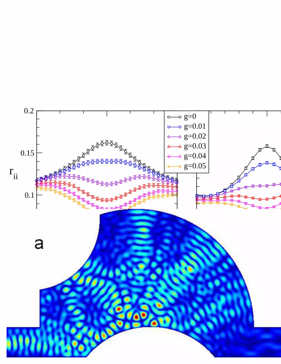
-0.003 0 0.003B

0.05

0.1

0.15

0.2

rii

g=0g=0.01g=0.02g=0.03g=0.04g=0.05

-0.001 0B

g=0g=0.01g=0.02g=0.03g=0.04g=0.05

a