Seediscussions,stats,andauthorprofilesforthispublicationat:https://www.researchgate.net/publication/259263943

Wave-inducedsetupinsidepermeablestructures

CONFERENCEPAPER·DECEMBER2012

DOI:10.9753/icce.v33.currents.43

CITATIONS

2

READS

24

2AUTHORS,INCLUDING:

MarcelR.A.vanGent

Deltares

90PUBLICATIONS617CITATIONS

SEEPROFILE

Availablefrom:MarcelR.A.vanGent

Retrievedon:03February2016

1

WAVE-INDUCED SETUP INSIDE PERMEABLE STRUCTURES

Peter Wellens1 and Marcel van Gent2

Coastal protection of land reclamation areas is often composed of rock or otherwise permeable material. Wave-induced setup inside permeable structures can be a problem for land reclamation areas if the design land level is too low. Wave-induced setup has not been studied extensively. In this study we use COMFLOW, a numerical model based on the Navier-Stokes equations employing the Volume-Of-Fluid method to displace the free surface, to quantify wave-induced setup inside permeable structures. The results are summarized in a conceptual design formula to determine wave-induced setup as a function of wave height Hm0 and rock diameter Dn50.

Keywords: waves; setup; permeable structure; Navier-Stokes; VOF

INTRODUCTION Detailed numerical methods based on the Navier-Stokes equations can be used in support of

experiments to understand the hydrodynamics in a flume or basin. Recently, we have developed a numerical method that includes flow through permeable structures. Similar methods may be found in Van Gent et al. (1994), Liu et al. (1999) and Lara et al. (2010). Our method is used to study wave interaction with permeable structures such as breakwaters. An example of a 3D simulation for a permeable structure is presented in Figure1. The figure shows a breakwater in along-axis loading conditions. The numerical method is incorporated in COMFLOW and has been presented in Wellens et al. (2010).

Figure 1. Example of a 3D simulation with a breakwater in along-axis loading conditions.

In Wellens et al. (2010), the numerical method was validated by means of a physical model test

results. In the physical model, several wave gauges were placed inside the structure, which registered the wave propagation through the structure. Wave propagation inside a permeable structure induces a non-linear, secondary phenomenon called internal wave setup. Wave setup inside the structure is defined as the time-averaged increase of the mean phreatic surface.

Wave-induced setup can cause problems in land reclamation areas if not duly accounted for. Figure 2 shows an example of a typical land reclamation area near the Port of Rotterdam: Maasvlakte 2 in the Netherlands. Land reclamation areas are often only slightly higher than a certain water level, in which HAT, a storm surge and wave setup as a result of wave breaking in the breaker zone are included. Wave setup inside the structure is often not included, which increases the risk of inundation as illustrated in Figure 3. Wave-induced setup has not been studied extensively and engineers are lacking guidelines with respect to wave-induced internal setup.

1 Deltares, P.O. Box 177, 2600 MH Delft, the Netherlands; peter.wellens@deltares.nl 2 Deltares, P.O. Box 177, 2600 MH Delft, the Netherlands; marcel.vangent@deltares.nl

COASTAL ENGINEERING 2012 2

In this paper, the numerical method is validated for the process of internal wave setup. With the

validated numerical method, research can be conducted with respect to the parameters that influence internal wave setup.

Figure 2. Typical land reclamation area: Maasvlakte 2 in the Netherlands.

Figure 3. Inundation of land reclamation area because of wave-induced internal setup in the coastal revetment. Dashed red lines represent the wave envelope; the continuous red line represents the increased mean free surface elevation inside the coastal revetment.

GOVERNING EQUATIONS For flow through permeable media, the Navier-Stokes equations need to account for the

permeability of the medium. With COMFLOW, we will not compute the flow through the pores themselves, i.e. the grid resolution in our simulations will be much coarser than the pores of the rock material that we wish to model. Therefore, a volume-averaged method is adopted, in which we assume that the properties of the permeable structure, such as the porosity, are homogenous throughout (part of) the structure. Besides porosity, we also need to account for the viscous interaction of the flow with the rocks in the permeable structure. We cannot represent all the (turbulent) boundary layers around the individual stones and will therefore model the viscous interaction with an additional volume averaged friction force in the Navier-Stokes equations that depends on the flow velocity. A similar approach is adopted in Darcy’s Law, which was adapted by Forchheimer to account for turbulent flows. The friction force is as follows:

( ) ( )ˆˆR u a b u u= + (1)

in which a is a Darcy-type coefficient, b is a Forchheimer-type coefficient and u is the actual flow

velocity in the permeable structure and not the bulk velocity. The expressions for a and b are based on Van Gent (1995). Friction force (1) is part of the extended Navier-Stokes equations for permeable flow.

COASTAL ENGINEERING 2012

3

The extended continuity equation for permeable flow is:

( ) 0ueÑ × = (2)

in which ε is the porosity. We assume constant viscosity and an incompressible fluid. Then the momentum equation reads:

( ) ( ) ( )u u u u p R u Ft

ee e n e e er

¶+Ñ× = Ñ × Ñ - Ñ - +

¶ (3)

Here, ν is the viscosity of the fluid, ρ is the density of the fluid, p is the pressure and F is an external force vector (such as, for instance, gravity).

DISCRETIZATION Eqs. (2) and (3) require discretization for the implementation in COMFLOW. In this section, the

discretization of the individual terms in the Navier-Stokes equation will be discussed. These terms will be combined later in the paragraph concerning the time discretization. In COMFLOW, a finite volume discretization has been adopted. To that end, we will now present the weak form of the Navier-Stokes equations. The continuity equation:

( )u n VeG

× ¶ò (4)

Here, n is the normal vector to the boundary of the control volume Г. The weak formulation of the momentum equation becomes:

( )

( ) ( )

udV u u n dSt

u ndS pndS R u dV FdV

e e

en e e er

W G

G G W W

¶+ × =

¶

Ñ × - - +

ò ò

ò ò ò ò (5)

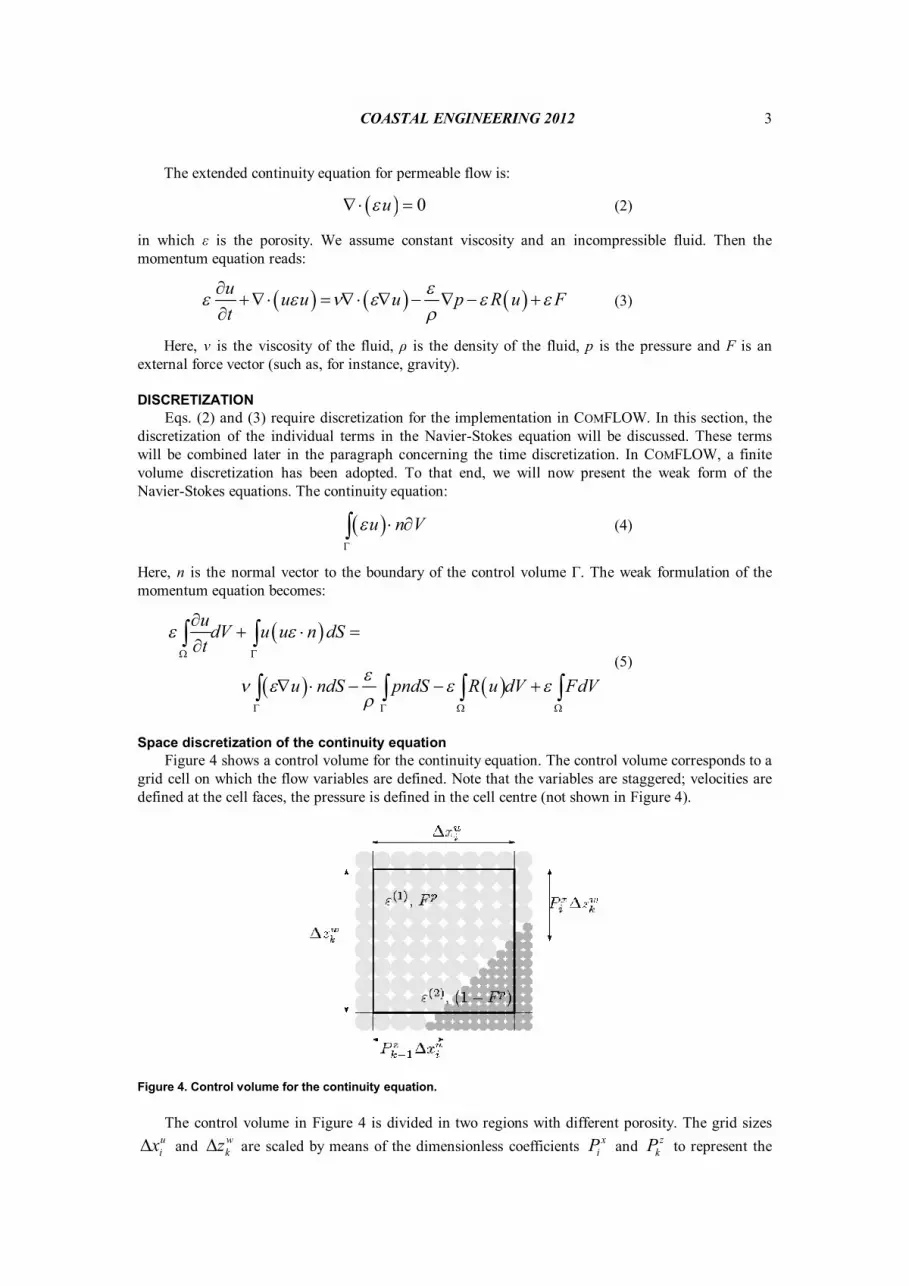
Space discretization of the continuity equation Figure 4 shows a control volume for the continuity equation. The control volume corresponds to a

grid cell on which the flow variables are defined. Note that the variables are staggered; velocities are defined at the cell faces, the pressure is defined in the cell centre (not shown in Figure 4).

Figure 4. Control volume for the continuity equation.

The control volume in Figure 4 is divided in two regions with different porosity. The grid sizes uixD and w

kzD are scaled by means of the dimensionless coefficients xiP and z

kP to represent the

COASTAL ENGINEERING 2012 4

outer dimensions of the two regions within the cell. The volumes of the regions are given by p u w

i kF x zD D and ( )1 p u wi kF x z- D D . Note, however, that the volume of the cell that is open for fluid,

in which we account for the porosity, is equal to:

( ) ( ) ( )( )1 2 1b p p u wi kF F F x ze e= + - D D (6)

We will determine the flow through the pores of the cell face indicated by i:

x wi i i ku A zF = D (7)

in which Φi represents the flux through the cell face with index i and:

( ) ( ) ( )1 2 1x x xi i iA P Pe e= + - (8)

is what we call an aperture. It is the area of the cell face that is open to fluid. The discrete equivalent of the continuity equation in Eq. (4) is as follows:

1 1 0i i k k- -F -F +F -F = (9)

And after substitution of all fluxes Φ around the circumference of the control volume, the discrete continuity equation reads:

( ) ( )1 1 1 1 0x x w z z ui i i i k k k k k iu A u A z w A w A x- - - -- D + - D = (10)

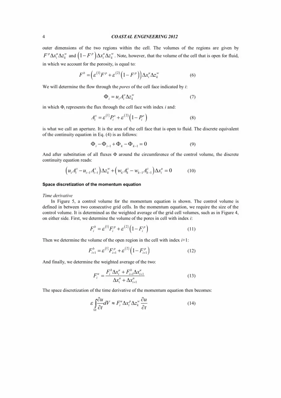
Space discretization of the momentum equation Time derivative

In Figure 5, a control volume for the momentum equation is shown. The control volume is defined in between two consecutive grid cells. In the momentum equation, we require the size of the control volume. It is determined as the weighted average of the grid cell volumes, such as in Figure 4, on either side. First, we determine the volume of the pores in cell with index i:

( ) ( ) ( )1 2 1b p pi i iF F Fe e= + - (11)

Then we determine the volume of the open region in the cell with index i+1:

( ) ( ) ( )1 21 1 11b p p

i i iF F Fe e+ + += + - (12)

And finally, we determine the weighted average of the two:

1 1

1

b u b uu i i i i

i u ui i

F x F xFx x

+ +

+

D + D=

D + D (13)

The space discretization of the time derivative of the momentum equation then becomes:

u p wi i k

u udV F x zt t

eW

¶ ¶» D D

¶ ¶ò (14)

COASTAL ENGINEERING 2012

5

Figure 5. Control volume for the momentum equation. Convective term

The Finite Volume discretization of the convective term is equal to the combination of fluxes over the boundary of the control volume:

( ) 1 1 1 12 2 2 2i i k ku u n dSe + - + -

G

× » F -F +F -Fò (15)

in which the fluxes through the right and the top control volume boundary are:

( ) ( )

( )

( ) ( )

( )

12

12

, 1, 1 , 1,

, , 1, 1, , 1,

, , 1,1 1, , , 1

, , 1, 1, , , 1

1 12 2

1 12 2

1 12 2

1 12 2

x x wi k i i k i k i k i ki

x x wi k i k i k i k k i k i k

z z ui k i k i i k i i k i kk

z z ui k i k i k i k i i k i k

u A u A z u u

u A u A z u u

w A w A x u u

w A w A x u u

x

x

+ + ++

+ + +

+ + ++

+ + +

F = + D + +

+ D -

F = + D + +

+ D -

(16)

Note in (16) that the parameter ξ determines the amount of upwind that is specified. The apertures A in Eq. (16) can be determined from Figure 5. As an example we will provide:

( ) ( ) ( )1 2 1x x xi i iA P Pe e= + - (17)

Viscous term

The discretization of the viscous term in this paper is relatively inaccurate compared to the other terms discussed here because it accounts for the porosity in a simplified manner. There are two reasons why we may assume that this discretization does not influence the results to a great extent. With COMFLOW we are primarily interested in wave loads as a result of steep waves; the type of flow in these waves is dominated by convection. In addition, inside permeable structures, the friction force term is by far dominant over the viscous term. For the discretization of the viscous term, we revert to the volume integral:

udVnW

Ñ×Ñò (18)

The divergence of the gradient of u is approximated as follows, see Figure 5:

COASTAL ENGINEERING 2012 6

1, , , 1, , 1 , , , 1

1 1

1 1i k i k i k i k i k i k i k i kp u u w p pi i i k k k

u u u u u u u uu

x x x z z z+ - + -

+ -

- - - -æ ö æ öÑ ×Ñ » Y = - + -ç ÷ ç ÷D D D D D Dè ø è ø

(19)

And Eq. (19) is multiplied by the volume of the momentum cell (see Eq. (13)) to obtain the full discretization of the viscous term:

u p wi i kudV F x zn n

W

Ñ×Ñ » D D Yò (20)

Pressure and force term

For the pressure term we adopt the following discretization, see Figure 5:

( ) ( ) ( ) ( ) ( )1 21 1

1 1x x wi i i i i i kpndS p p P p p P ze e e

r r + +W

é ù» - + - - Dë ûò (21)

For the force term, a discretization is adopted in such a way that in hydrostatic circumstances the

discrete form of 1 p FrÑ = is satisfied. The discretization of the force term in x-direction then becomes:

( ) ( ) ( )1 2 1x x p wx x i x i i kF dV F P F P x ze e

W

é ù» + - D Dë ûò (22)

Friction force term

For the integration of the friction force term over the control volume, we adopt a weighted average method. The friction force in the control volume with index i (see Figure 5) is:

( ) ( ) ( ) ( )( ) ( ) ( )( )( ) ( ) ( )( )( )

12

1 1 1 2 21 2

2 2 2 2 2

11

1

pi c ii p p

i i

pi c i i

R u a b u w FF F

a b u w F u

ee e

e

-é= + + +êë+ -

ù+ + - úû

(23)

The friction force in the cell with index i+1:

( ) ( ) ( ) ( )( ) ( ) ( )( )( ) ( ) ( )( )( )

12

1 1 1 2 211 2

1 1

2 2 2 2 21

11

1

pi c ii p p

i i

pi c i i

R u a b u w FF F

a b u w F u

ee e

e

+++ +

+

é= + + +êë+ -

ù+ + - úû

(24)

in which wc is approximated as the simple average of the vertical velocities at the position of ui:

( ), , 1 1, 1, 114c i k i k i k i kw w w w w- + + -= + + + (25)

Then, the total discretization of the friction force term becomes:

( )1 12 2

1

1

u ui ii iu p w

i i k u ui i

R x R xR u dV F x z

x x+- +

+W

D + D» D D

D +Dò (26)

COASTAL ENGINEERING 2012

7

Time discretization of the momentum equation The space discretization of the continuity equation and the momentum equation can be written in

matrix form and combined with a Forward Euler time integration:

( )

1

11 1

0

1 ˆ

n

n nn n n n n

M

C D G F Rt

e

e e e e e enr

+

++ +

=

-W = - + - + -

D

u

u u u u u p u (27)

In (27), the subscripts ε indicate that we have accounted for the porosity in the space discretization. Note that the convective term is non-linear, i.e. the coefficients of the matrix depend on the velocity u. Also note in this equation that the convective and viscous term are explicit and the pressure term and the friction force term are implicit. We introduce an auxiliary vector field nu% :

( )( )1n n n n nt C D Fe e e en-= -D W - -u u u u u% (28)

combine it with the momentum equation and rearrange terms to obtain:

11 1 1 1ˆ1n n ntt R Ge e e er

-+ - - +æ öDé ù= + D W - Wç ÷ë û è ø

u u p% (29)

Eq. (29) is substituted into the discrete continuity equation. The result is a Poisson equation for the pressure that reads:

1 11 1 1 1ˆ ˆ1 1n nM t R G M t R

te e e e e e e er- -

- - + -é ù é ù+ D W W = + D Wë û ë ûDp u% (30)

From this equation the pressure is solved, after which the velocities at the new time level are found from (29).

VALIDATION Experimental results are used to validate the implementation of permeable flow in COMFLOW.

We will use the experiment presented in Wellens et al. (2010), in which COMFLOW was validated for the wave height inside the structure, for the purpose of validating COMFLOW for internal setup. We will consider regular waves. The permeable structure represents a breakwater with a core of relatively fine material and an armour layer with relatively coarse rock. The outer measures of the structure are shown in Figure 6. The base of the structure is about 3 meters wide, the top of the structure 0.35m wide at an elevation of 0.93m. The slopes are 1:1.5. The mean free surface in the experiments was at an elevation of 0.60m

Figure 6. Outer measures of the permeable structure. The breakwater consists of an armour layer and a core.

COASTAL ENGINEERING 2012 8

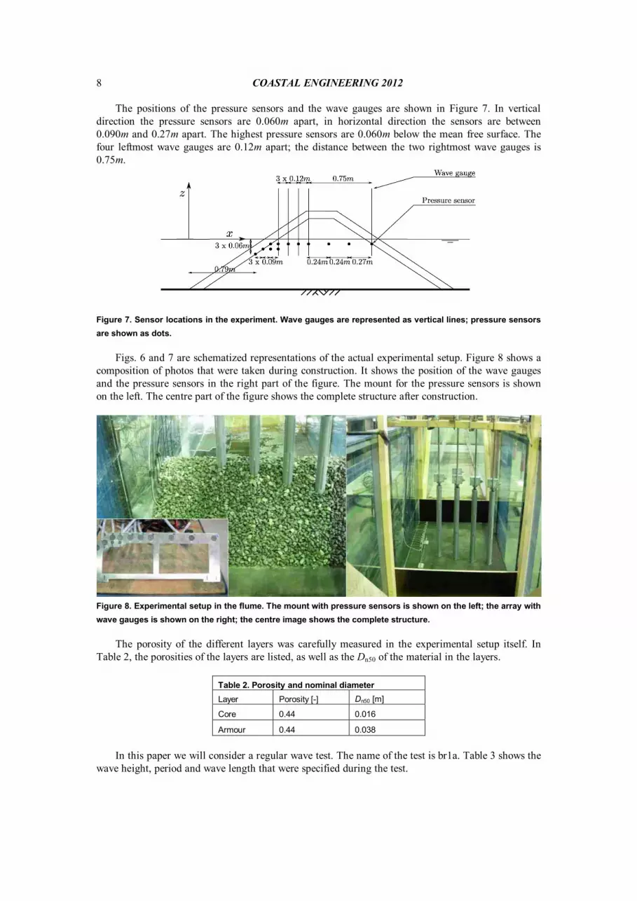
The positions of the pressure sensors and the wave gauges are shown in Figure 7. In vertical direction the pressure sensors are 0.060m apart, in horizontal direction the sensors are between 0.090m and 0.27m apart. The highest pressure sensors are 0.060m below the mean free surface. The four leftmost wave gauges are 0.12m apart; the distance between the two rightmost wave gauges is 0.75m.

Figure 7. Sensor locations in the experiment. Wave gauges are represented as vertical lines; pressure sensors are shown as dots.

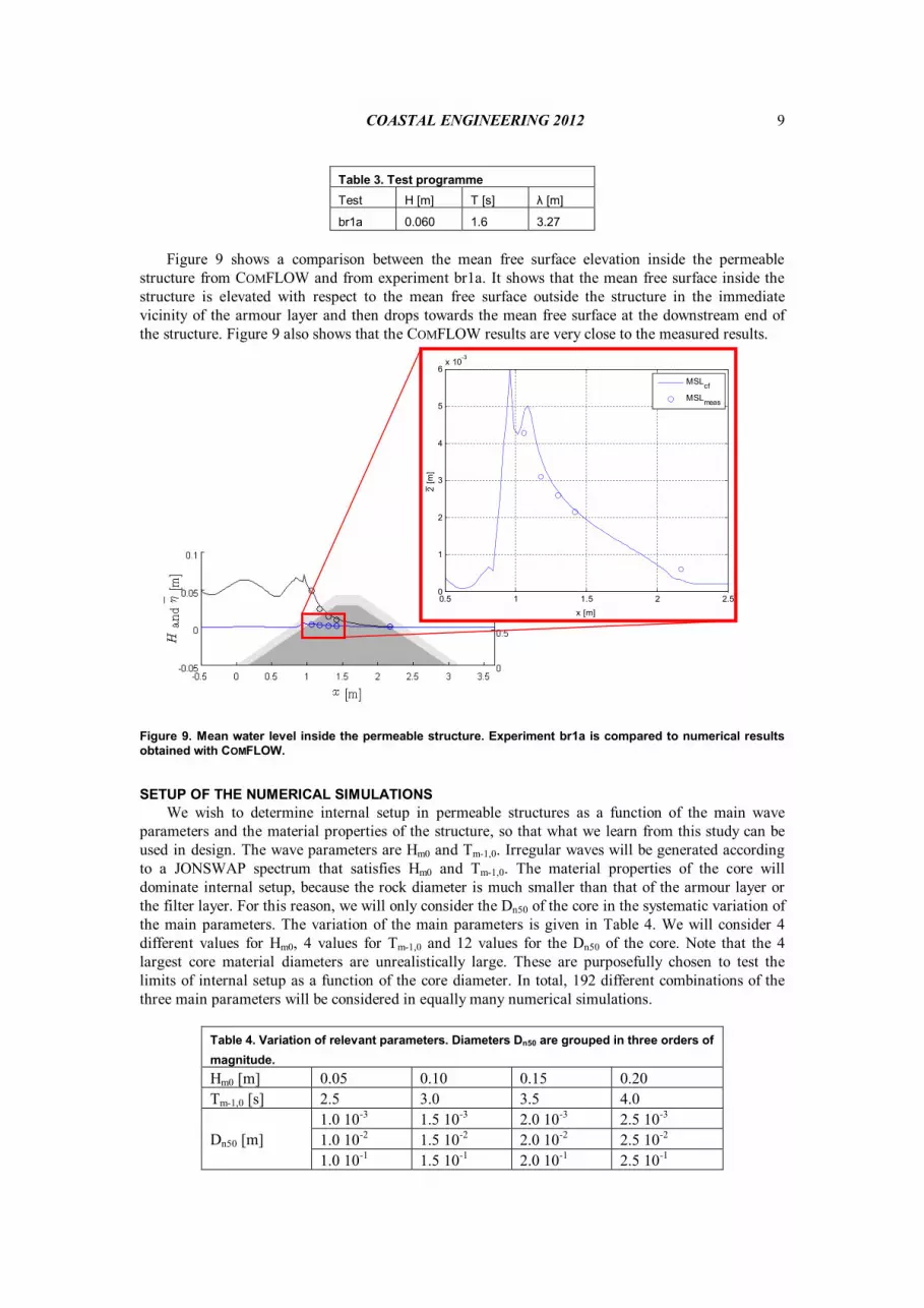
Figs. 6 and 7 are schematized representations of the actual experimental setup. Figure 8 shows a composition of photos that were taken during construction. It shows the position of the wave gauges and the pressure sensors in the right part of the figure. The mount for the pressure sensors is shown on the left. The centre part of the figure shows the complete structure after construction.

Figure 8. Experimental setup in the flume. The mount with pressure sensors is shown on the left; the array with wave gauges is shown on the right; the centre image shows the complete structure.

The porosity of the different layers was carefully measured in the experimental setup itself. In Table 2, the porosities of the layers are listed, as well as the Dn50 of the material in the layers.

Table 2. Porosity and nominal diameter Layer Porosity [-] Dn50 [m]

Core 0.44 0.016

Armour 0.44 0.038

In this paper we will consider a regular wave test. The name of the test is br1a. Table 3 shows the wave height, period and wave length that were specified during the test.

COASTAL ENGINEERING 2012

9

Table 3. Test programme Test H [m] T [s] λ [m]

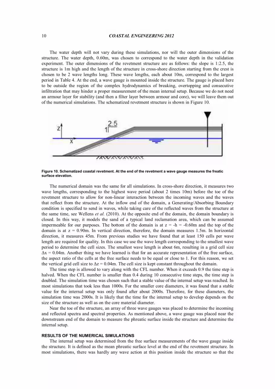
br1a 0.060 1.6 3.27 Figure 9 shows a comparison between the mean free surface elevation inside the permeable

structure from COMFLOW and from experiment br1a. It shows that the mean free surface inside the structure is elevated with respect to the mean free surface outside the structure in the immediate vicinity of the armour layer and then drops towards the mean free surface at the downstream end of the structure. Figure 9 also shows that the COMFLOW results are very close to the measured results.

Figure 9. Mean water level inside the permeable structure. Experiment br1a is compared to numerical results obtained with COMFLOW.

SETUP OF THE NUMERICAL SIMULATIONS We wish to determine internal setup in permeable structures as a function of the main wave

parameters and the material properties of the structure, so that what we learn from this study can be used in design. The wave parameters are Hm0 and Tm-1,0. Irregular waves will be generated according to a JONSWAP spectrum that satisfies Hm0 and Tm-1,0. The material properties of the core will dominate internal setup, because the rock diameter is much smaller than that of the armour layer or the filter layer. For this reason, we will only consider the Dn50 of the core in the systematic variation of the main parameters. The variation of the main parameters is given in Table 4. We will consider 4 different values for Hm0, 4 values for Tm-1,0 and 12 values for the Dn50 of the core. Note that the 4 largest core material diameters are unrealistically large. These are purposefully chosen to test the limits of internal setup as a function of the core diameter. In total, 192 different combinations of the three main parameters will be considered in equally many numerical simulations.

Table 4. Variation of relevant parameters. Diameters Dn50 are grouped in three orders of magnitude. Hm0 [m] 0.05 0.10 0.15 0.20 Tm-1,0 [s] 2.5 3.0 3.5 4.0

1.0 10-3 1.5 10-3 2.0 10-3 2.5 10-3 1.0 10-2 1.5 10-2 2.0 10-2 2.5 10-2 Dn50 [m] 1.0 10-1 1.5 10-1 2.0 10-1 2.5 10-1

0.5 1 1.5 2 2.50

1

2

3

4

5

6x 10-3

x [m]

2[m

]

MSLcf

MSLmeas

COASTAL ENGINEERING 2012 10

The water depth will not vary during these simulations, nor will the outer dimensions of the

structure. The water depth, 0.60m, was chosen to correspond to the water depth in the validation experiment. The outer dimensions of the revetment structure are as follows: the slope is 1:2.5, the structure is 1m high and the length of the structure in cross-shore direction starting from the crest is chosen to be 2 wave lengths long. These wave lengths, each about 10m, correspond to the largest period in Table 4. At the end, a wave gauge is mounted inside the structure. The gauge is placed here to be outside the region of the complex hydrodynamics of breaking, overtopping and consecutive infiltration that may hinder a proper measurement of the mean internal setup. Because we do not need an armour layer for stability (and then a filter layer between armour and core), we will leave them out of the numerical simulations. The schematized revetment structure is shown in Figure 10.

Figure 10. Schematized coastal revetment. At the end of the revetment a wave gauge measures the freatic surface elevation.

The numerical domain was the same for all simulations. In cross-shore direction, it measures two wave lengths, corresponding to the highest wave period (about 2 times 10m) before the toe of the revetment structure to allow for non-linear interaction between the incoming waves and the waves that reflect from the structure. At the inflow end of the domain, a Generating/Absorbing Boundary condition is specified to send in waves, while taking care of the reflected waves from the structure at the same time, see Wellens et al. (2010). At the opposite end of the domain, the domain boundary is closed. In this way, it models the sand of a typical land reclamation area, which can be assumed impermeable for our purposes. The bottom of the domain is at z = -h = -0.60m and the top of the domain is at z = 0.90m. In vertical direction, therefore, the domain measures 1.5m. In horizontal direction, it measures 45m. From previous studies we have found that at least 150 cells per wave length are required for quality. In this case we use the wave length corresponding to the smallest wave period to determine the cell sizes. The smallest wave length is about 6m, resulting in a grid cell size Δx = 0.04m. Another thing we have learned is that for an accurate representation of the free surface, the aspect ratio of the cells at the free surface needs to be equal or close to 1. For this reason, we set the vertical grid cell size to Δz = 0.04m. The cell size is kept constant throughout the domain.

The time step is allowed to vary along with the CFL number. When it exceeds 0.9 the time step is halved. When the CFL number is smaller than 0.4 during 10 consecutive time steps, the time step is doubled. The simulation time was chosen such that a stable value of the internal setup was reached. In most simulations that took less than 1000s. For the smaller core diameters, it was found that a stable value for the internal setup was only found after about 2000s. Therefore, for these diameters, the simulation time was 2000s. It is likely that the time for the internal setup to develop depends on the size of the structure as well as on the core material diameter.

Near the toe of the structure, an array of three wave gauges was placed to determine the incoming and reflected spectra and spectral properties. As mentioned above, a wave gauge was placed near the downstream end of the domain to measure the phreatic surface inside the structure and determine the internal setup.

RESULTS OF THE NUMERICAL SIMULATIONS The internal setup was determined from the free surface measurements of the wave gauge inside

the structure. It is defined as the mean phreatic surface level at the end of the revetment structure. In most simulations, there was hardly any wave action at this position inside the structure so that the

COASTAL ENGINEERING 2012

11

mean phreatic surface could be read from the registration of the wave gauge, see Figure 11 for a registration of the free surface as a function of time for one of the simulations. In others, for the larger core material diameters, some wave action remained and the mean surface position was determined as the average of the last 10 wave periods.

From the wave gauge array at the toe of the structure, the incoming wave height Hm0, in and the period Tm-1,0; in were determined.

Figure 11. Internal setup as it develops over time (in irregular waves).

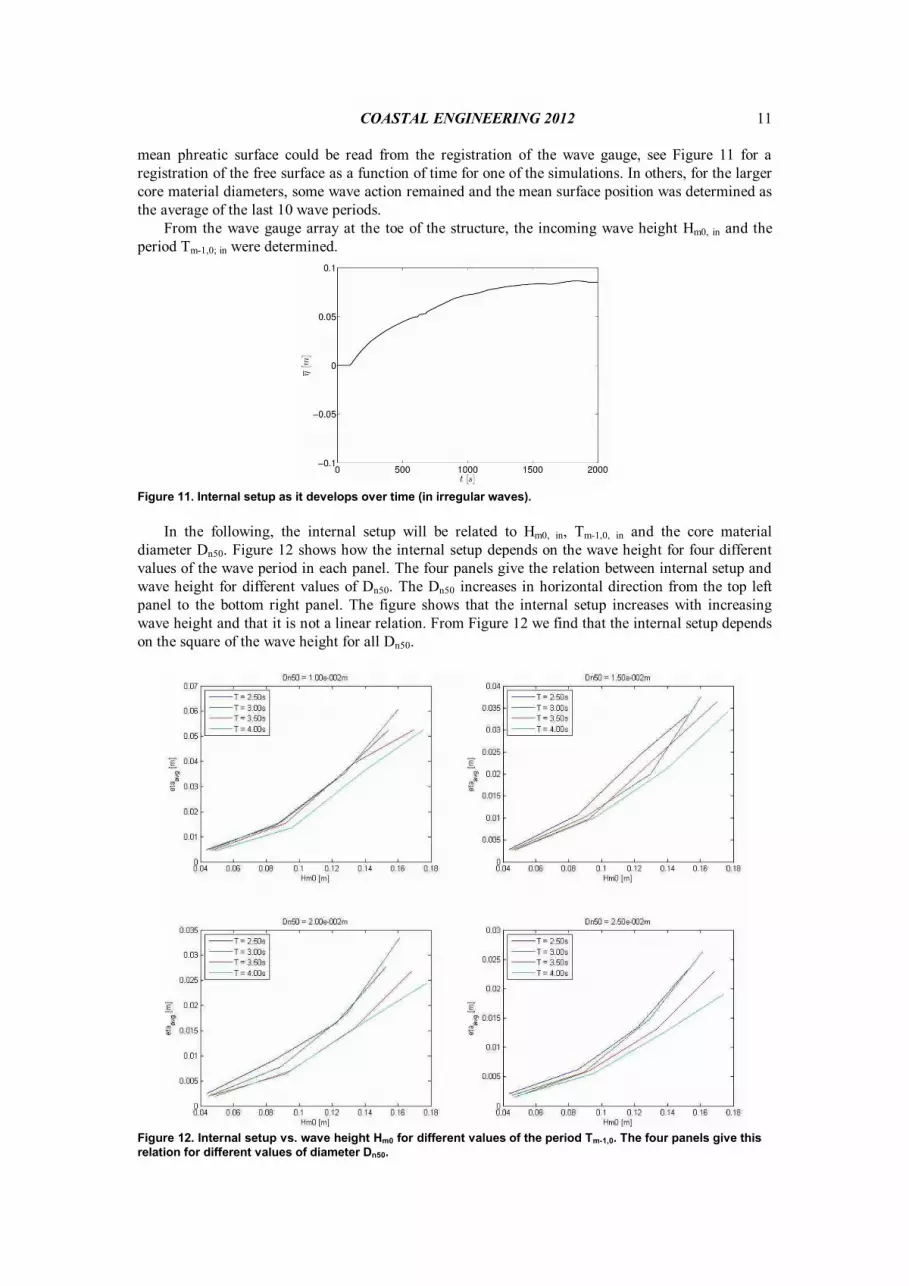
In the following, the internal setup will be related to Hm0, in, Tm-1,0, in and the core material diameter Dn50. Figure 12 shows how the internal setup depends on the wave height for four different values of the wave period in each panel. The four panels give the relation between internal setup and wave height for different values of Dn50. The Dn50 increases in horizontal direction from the top left panel to the bottom right panel. The figure shows that the internal setup increases with increasing wave height and that it is not a linear relation. From Figure 12 we find that the internal setup depends on the square of the wave height for all Dn50.

Figure 12. Internal setup vs. wave height Hm0 for different values of the period Tm-1,0. The four panels give this relation for different values of diameter Dn50.

COASTAL ENGINEERING 2012 12

In Figure 13, internal setup is plotted against the wave period Tm-1,0 for four different values of the

wave height. The four panels give this relation for four different values of Dn50. The Dn50 increases from the top left panel to the bottom right panel in horizontal direction. Here, if we consider the top left panel of Figure 13, we find that the variation with the period is small and inconsistent for the different wave heights. This behaviour for the internal setup as a function of the period is the same for each diameter. No trend for internal setup as a function of period can be identified and therefore we will not include the wave period in estimates of internal setup.

Figure 13. Internal setup vs. wave period Tm-1,0 for different values of the wave height Hm0. The four panels give this relation for different values of diameter Dn50.

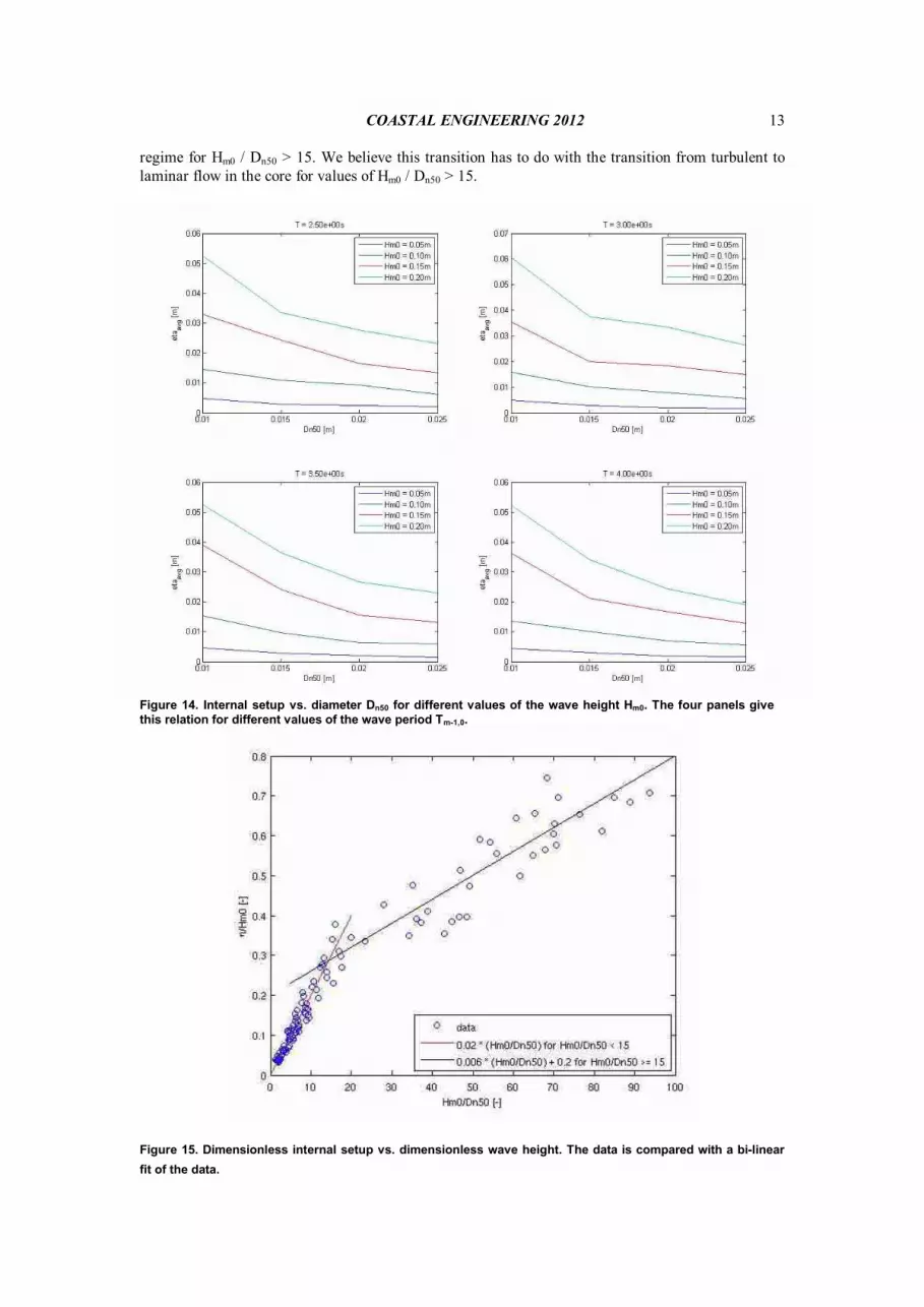
In Figure 14, internal setup is plotted against the core material diameter Dn50 for different values of the wave height. The four panels show internal setup versus Dn50 for different values of the wave period. The top left panel shows that internal setup decreases for increasing values of Dn50. The behaviour of internal setup versus Dn50 is consistent for all Hm0 and Tm-1,0. From Figure 14, we find that internal setup depends on Dn50 as 1 over Dn50.

Summarizing the conclusions from Figures 12 to 14 we can derive the following relation:

0

0 50

m

m n

HH Dh

: (31)

in which η over Hm0 is the dimensionless internal setup.

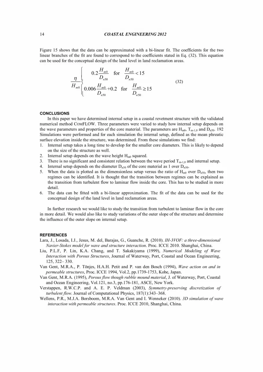
In Eq. (31), we see that the dimensionless setup has a linear relation with the wave height over core diameter ratio. In Figure 15, the results from all simulations are plotted according to the relation found in Eq. (31). Two regimes can be identified: there is a regime for Hm0 / Dn50 < 15 and a distinct

COASTAL ENGINEERING 2012

13

regime for Hm0 / Dn50 > 15. We believe this transition has to do with the transition from turbulent to laminar flow in the core for values of Hm0 / Dn50 > 15.

Figure 14. Internal setup vs. diameter Dn50 for different values of the wave height Hm0. The four panels give this relation for different values of the wave period Tm-1,0.

Figure 15. Dimensionless internal setup vs. dimensionless wave height. The data is compared with a bi-linear fit of the data.

COASTAL ENGINEERING 2012 14

Figure 15 shows that the data can be approximated with a bi-linear fit. The coefficients for the two linear branches of the fit are found to correspond to the coefficients stated in Eq. (32). This equation can be used for the conceptual design of the land level in land reclamation areas.

0 0

50 50

0 00

50 50

0.2 for 15

0.006 +0.2 for 15

m m

n n

m mm

n n

H HD D

H HHD D

hì <ïïíï ³ïî

(32)

CONCLUSIONS In this paper we have determined internal setup in a coastal revetment structure with the validated

numerical method COMFLOW. Three parameters were varied to study how internal setup depends on the wave parameters and properties of the core material. The parameters are Hm0, Tm-1,0 and Dn50. 192 Simulations were performed and for each simulation the internal setup, defined as the mean phreatic surface elevation inside the structure, was determined. From these simulations we find: 1. Internal setup takes a long time to develop for the smaller core diameters. This is likely to depend

on the size of the structure as well. 2. Internal setup depends on the wave height Hm0 squared. 3. There is no significant and consistent relation between the wave period Tm-1,0 and internal setup. 4. Internal setup depends on the diameter Dn50 of the core material as 1 over Dn50. 5. When the data is plotted as the dimensionless setup versus the ratio of Hm0 over Dn50, then two

regimes can be identified. It is thought that the transition between regimes can be explained as the transition from turbulent flow to laminar flow inside the core. This has to be studied in more detail.

6. The data can be fitted with a bi-linear approximation. The fit of the data can be used for the conceptual design of the land level in land reclamation areas. In further research we would like to study the transition from turbulent to laminar flow in the core

in more detail. We would also like to study variations of the outer slope of the structure and determine the influence of the outer slope on internal setup.

REFERENCES Lara, J., Losada, I.J., Jesus, M. del, Barajas, G., Guanche, R. (2010). IH-3VOF: a three-dimensional

Navier-Stokes model for wave and structure interaction. Proc. ICCE 2010. Shanghai, China. Liu, P.L.F, P. Lin, K.A. Chang, and T. Sakakiyama (1999), Numerical Modeling of Wave

Interaction with Porous Structures, Journal of Waterway, Port, Coastal and Ocean Engineering, 125, 322– 330.

Van Gent, M.R.A., P. Tönjes, H.A.H. Petit and P. van den Bosch (1994), Wave action on and in permeable structures, Proc. ICCE 1994, Vol.2, pp.1739-1753, Kobe, Japan.

Van Gent, M.R.A. (1995), Porous flow though rubble mound material, J. of Waterway, Port, Coastal and Ocean Engineering, Vol.121, no.3, pp.176-181, ASCE, New York.

Verstappen, R.W.C.P. and A. E. P. Veldman (2003), Symmetry-preserving discretization of turbulent flow. Journal of Computational Physics, 187(1):343–368.

Wellens, P.R., M.J.A. Borsboom, M.R.A. Van Gent and I. Wenneker (2010). 3D simulation of wave interaction with permeable structures. Proc. ICCE 2010, Shanghai, China.