water resources in lake tana basin - macau
TRANSCRIPT
Institut für Natur- und Ressorcenschutz
Christian-Albrechts-Universität zu Kiel
Water Resources in Lake Tana Basin:
Analysis of hydrological time series data and
impact of climate change with emphasis on
groundwater, Upper Blue Nile Basin, Ethiopia
Dissertation
Zur Erlangung des Doktorgrades der Agrar- und
Ernährungswissenschaftliche Fakultät
der Christian Albrechts Universität zu Kiel
Vorgelegt von
M.Sc. Tibebe Belete Tigabu
geboren im 13 März 1981
Kiel, 2020
Dean: Prof. Dr. Christian Henning
1. Erste Gutachterin: Prof. Dr. Nicola Fohrer
2. Zweite Gutachterin: Prof. Dr. Hans-Rudolf Bork
Tag der mündlichen Prüfung : 17.06.2020
i
Abstract
Ethiopia is a source region of the Nile River and famous for its water resources potential.
The available annual average water per person per year is estimated to be 1575 m3.
However, the water is not available at the time and place where it is required due to the
large spatial and temporal variations in rainfall and a lack of the required technology and
infrastructure. Therefore, the Ethiopian government has selected different areas as
development corridors to achieve its development and transformation agenda. Among
others, the Lake Tana basin is one of the development corridor areas primarily due to its
groundwater and surface water potential. The total catchment area of the Lake Tana basin
is 15,321 km². The climate is influenced by the movement of the inter-tropical
convergence zone (ITCZ) resulting in a high seasonality of rainfall with a rainy season
between June and September. However, the scientific understanding of the hydrologic
response to intensive agriculture, the interconnection of groundwater and surface water,
and future perspectives of the water availability under global climate change is limited.
Therefore, the main aim of this study is to improve our understanding of past, present,
and future hydrologic conditions in three sub catchments of the Lake Tana basin,
Gilgelabay, Gumara, and Ribb. Different sequential methodological approaches were
followed to achieve the research objective. The spatial and temporal patterns of the
hydrologic conditions during the last half century were analysed based on long-term
hydrological and climatological data between 1960 and 2015 using the Mann-Kendal
trend test, auto- and cross-correlation, and Tukey multiple mean comparison tests.
Furthermore, the semi-distributed hydrologic model SWAT (Soil and Water Assessment
Tools) and an integrated surface water and groundwater model (SWAT-MODFLOW),
which is a hybrid of the SWAT model and MODFLOW (a three-dimensional finite
difference groundwater model) were applied. The hydrologic models were calibrated and
ii
validated to minimize uncertainties. The mid-term and long-term development of the 21st
century was modelled using projected rainfall and temperature data of an ensemble of
regional climate models under the scenarios of Representative Concentration Pathways
RCP4.5 and RCP8.5.
Results from the long-term time series analyses revealed that the hydrologic condition in
the study area is highly variable both at spatial and temporal scales. The rainfall and
streamflow patterns showed high seasonal anomalies. Most of the peak rainfall and
streamflow events occur during the wet season (June to September); all other months are
characterized as dry season (October to May) with less rainfall and low flow. The
statistical tests indicated that the overall annual rainfall in the Lake Tana basin did not
change significantly, but there are slight changes. The streamflow increased significantly
for Gumara and Megech, the Lake outflow decreased during the 2000s to 2010s. The
lake level dropped abruptly since the beginning of 2000s and did not recover yet.
Results of the SWAT model also proved that the hydrologic condition in the study area
is highly variable both spatially and seasonally. The dominant agricultural crops showed
variable influences on the major water balance components. Groundwater recharge was
relatively high on agricultural land covered by cereal crops like teff and millet, whereas
surface runoff was significantly enhanced on cultivated land covered by leguminous
crops like peas. Compared to Gilgelabay and Ribb, Gumara catchment showed more
surface runoff. Groundwater discharge contributes substantial amount to the streamflow
in all the three catchments.
The interconnectivity between the groundwater and surface water was assessed with the
coupled hydrologic model SWAT-MODFLOW. The groundwater-surface water
iii
interactions showed significant spatial and temporal variabilities. There were also
different dynamics of groundwater-surface interaction between the three catchments. The
annual exchange rate was dominated by flow from the aquifer to the stream in the
Gilgelabay catchment, while bidirectional flow was observed in the Gumara and Ribb
catchments. Compared to the annual groundwater-surface water interaction, the daily
interaction was more dynamic.
Possible future changes of the major water balance components in the Lake Tana basin
were simulated with the two greenhouse gas concentration pathways, RCP4.5 and
RCP8.5. The expected increases of the ensemble mean temperature in the study area are
likely to be higher than the global average, while the expected changes in rainfall are not
significant. Relative to the baseline average, the ensemble mean actual
evapotranspiration are likely to decrease in both catchments for both periods. Likewise,
groundwater contribution to the streamflow is likely to decrease in both future periods
under both scenarios. Unlike actual evapotranspiration and groundwater contribution to
the streamflow, surface runoff is expected to increase significantly for both periods under
both scenarios. This is due to the expected high variability of rainfall intensity and
seasonality during the two future periods.
Modelling and time series analyses enhances our understanding of past, current and
possible future hydrologic conditions in the study area. Overall, outputs revealed that
considerable spatio-temporal changes had occurred for the hydrology of Lake Tana Basin
during the last half century and more changes are also expected in the future.
Consequently, the results of this PhD dissertation can contribute to develop future water
management plans in the region and beyond.
iv
Zusammenfassung
Äthiopien ist eine Quellregion des Nils und bekannt für sein großen Wasserressourcen.
Die verfügbare Wassermenge pro Person und Jahr wird auf durchschnittlich 1575 m³
geschätzt. Das Wasser ist jedoch aufgrund der großen räumlichen und zeitlichen
Schwankungen der Niederschläge und aufgrund des Mangels von erforderlicher
Infrastruktur und Technologie nicht zu der Zeit und an dem Ort verfügbar, an dem es
benötigt wird. Um ihre Entwicklungs- und Transformationsagenda zu erreichen, hat die
äthiopische Regierung verschiedene Regionen im Land als Entwicklungskorridore
ausgewählt. Unter anderem ist das Einzugsgebiet des Tanasees aufgrund seiner
Ressourcen von Grund- und Oberflächenwasser Teil des Entwicklungskorridors. Das
gesamte Einzugsgebiet des Tanasees hat eine Fläche von 15 321 km². Das Klima der
Region wird durch die Verlagerung der innertropischen Konvergenzzone bestimmt, die
in einer ausgeprägten Saisonalität des Niederschlags mit einer Regenzeit von Juni bis
September resultiert. Das wissenschaftliche Verständnis bezüglich der hydrologischen
Reaktion auf die intensive Landwirtschaft, der Verbindung von Grund- und
Oberflächenwasser und der zukünftigen Wasserverfügbarkeit unter dem Einfluss des
globalen Klimawandels ist jedoch begrenzt. Daher ist das Ziel dieser Dissertation, die
vergangenen, gegenwärtigen und zukünftigen hydrologischen Bedingungen in drei
Teileinzugsgebieten des Tanasee-Einzugsgebiets, den Teileinzugsgebieten Gilgelabay,
Gumara und Ribb, besser zu verstehen. Um das Forschungsziele zu erreichen, wurden
nacheinander verschiedene methodische Ansätze verfolgt. Die räumlichen und zeitlichen
Muster der hydrologischen Bedingungen während des letzten halben Jahrhunderts
wurden auf der Grundlage langfristiger hydrologischer und klimatologischer Daten
zwischen 1960 und 2015 unter Verwendung des Mann-Kendal-Trendtests, der Auto- und
Kreuzkorrelation und der Tukey-Mehrfachmittelwertvergleichstests analysiert. Darüber
v
hinaus wurden das hydrologische Modell SWAT (Soil and Water Assessment Tools) und
ein integriertes Oberflächen- und Grundwassermodell (SWAT-MODFLOW), das eine
Kopplung zwischen den Modellen SWAT und MODFLOW (ein dreidimensionales
Finite-Differenzen-Grundwassermodell) darstellt, angewandt. Die hydrologischen
Modelle wurden kalibriert und validiert, um Unsicherheiten zu minimieren. Die mittel-
und langfristige Entwicklung des 21. Jahrhunderts wurde anhand von prognostizierten
Niederschlags- und Temperaturdaten eines Ensembles regionaler Klimamodelle unter
den Szenarien ‚repräsentativer Konzentrationspfade‘ RCP4.5 und RCP8.5 modelliert.
Die Ergebnisse aus den Zeitreihenanalysen zeigten, dass der hydrologische Zustand im
Untersuchungsgebiet sowohl auf räumlicher als auch auf zeitlicher Ebene sehr variabel
ist. Die Niederschlags- und Abflussmuster wiesen hohe saisonale Anomalien auf. Die
meisten Spitzenwerte der Niederschlags- und Abflussereignisse treten während der
Regenzeit (Juni bis September) auf. Alle anderen Monate sind als Trockenzeit (Oktober
bis Mai) durch weniger Niederschlag und geringen Abfluss gekennzeichnet. Die
statistischen Tests ergaben, dass sich die jährliche Gesamtregenmenge im Tanasee-
Einzugsgebiet nicht wesentlich verändert hat, aber es dennoch leichte Veränderungen
gibt. Der Abfluss nahm in den Teileinzugsgebieten Gumara und Megech deutlich zu.
Hingegen nahm der Abfluss des Sees von den 2000er zu den 2010er Jahren ab. Der
Seewasserspiegel fiel seit Anfang der 2000er Jahre abrupt und erholte sich seitdem nicht
mehr.
Die Ergebnisse des SWAT-Modells zeigten ebenfalls, dass der hydrologische Zustand
im Untersuchungsgebiet sowohl räumlich als auch jahreszeitlich sehr variabel ist. Die
vorherrschenden landwirtschaftlichen Kulturen zeigten variable Einflüsse auf die
wichtigsten Wasserhaushaltskomponenten. Die Grundwasserneubildung war auf
vi
landwirtschaftlich genutzten Flächen, die mit Getreidekulturen wie Teff und Hirse
bedeckt waren, relativ hoch, während der Oberflächenabfluss auf landwirtschaftlich
genutzten Flächen, die mit Leguminosen wie Erbsen bedeckt waren, signifikant erhöht
war. Im Vergleich zu Gilgelabay und Ribb zeigte das Gumara-Einzugsgebiet mehr
Oberflächenabfluss. Der Grundwasserabfluss trägt in allen drei Einzugsgebieten in
erheblichem Maße zum Abfluss bei.
Die Wechselwirkung zwischen Grundwasser und Oberflächenwasser wurde mit dem
gekoppelten hydrologischen Modell SWAT-MODFLOW untersucht. Sie zeigte eine
signifikante räumliche und zeitliche Variabilität. Zwischen den drei Einzugsgebieten gab
es eine unterschiedliche Dynamik der Interaktion von Grundwasser und
Oberflächenwasser. Im Gilgelabay-Einzugsgebiet wurde der jährliche Austausch durch
die Fließrichtung vom Aquifer zum Fließgewässer dominiert, während in den
Einzugsgebieten Gumara und Ribb bidirektionale Flüsse beobachtet wurden. Im
Vergleich zur jährlichen Interaktion von Grundwasser und Oberflächenwasser war die
tägliche Interaktion dynamischer.
Mögliche zukünftige Veränderungen der wichtigsten Wasserhaushaltskomponenten im
Tanasee-Einzugsgebiet wurden mit den beiden Szenarien ‚repräsentativer
Konzentrationspfade’ RCP4.5 und RCP8.5 simuliert. Der Anstieg der Ensemble-
Mitteltemperatur im Untersuchungsgebiet ist höher als der globale Durchschnitt,
während die Veränderung der Niederschläge nicht signifikant ist. Relativ zum
Durchschnitt des Referenzlaufs (baseline) zeigen die Ensemble-Mittelwerte, dass die
tatsächliche Evapotranspiration in beiden Einzugsgebieten für beide Perioden abnimmt.
vii
Ebenso nimmt der Anteil des Grundwassers am Abfluss in beiden zukünftigen Perioden
und in beiden Szenarien ab. Im Gegensatz zur tatsächlichen Evapotranspiration und zum
Grundwasseranteils am Abfluss wird sich der Oberflächenabfluss in beiden Szenarien für
beide Zeiträume voraussichtlich deutlich erhöhen. Dies ist auf die hohe Variabilität der
Niederschlagsintensität und Saisonalität während der beiden zukünftigen Perioden
zurückzuführen.
Modellierung und Zeitreihenanalysen verbessern das Verständnis der vergangenen,
aktuellen und möglichen zukünftigen hydrologischen Bedingungen im
Untersuchungsgebiet. Insgesamt zeigen die Ergebnisse, dass sich die Hydrologie des
Tanasee-Einzuggebiets im letzten halben Jahrhundert räumlich und zeitlich erheblich
verändert hat und auch in Zukunft deutliche Veränderungen zu erwarten sind. Folglich
können die Erkenntnisse dieser Dissertation zur Entwicklung von zukünftigen
Wassermanagementplänen in der Region und darüber hinaus beitragen.
viii
Table of contents Abstract ............................................................................................................................. i
Zusammenfassung................................................................................................................... iv
Table of contents ................................................................................................................... viii
1. General introduction ........................................................................................................ 1
1.1. Background ................................................................................................................. 1
1.2. Analysis of hydrometeorological time series .............................................................. 5
1.3. Hydrological modeling ................................................................................................ 6
1.4. Groundwater dynamics and climate change ................................................................ 7
1.5. Statement of the problem and research questions ..................................................... 11
1.6. Thesis structure ......................................................................................................... 14
2. Statistical analysis of rainfall and streamflow time series in the Lake Tana Basin,
Ethiopia .......................................................................................................................... 16
Abstract ............................................................................................................................... 17
2.1. Introduction ............................................................................................................... 18
2.2. Materials and Methods .............................................................................................. 20
2.2.1. General overview of the study area ................................................................... 20
2.2.2. Data Analysis ..................................................................................................... 22
2.3. Results and discussion ............................................................................................... 26
2.3.1. Rainfall analysis ................................................................................................. 26
2.3.2. Stream flow analysis .......................................................................................... 32
2.3.3. Lake water level analysis ................................................................................... 39
2.4. Conclusions ............................................................................................................... 41
3. Modeling the impact of agricultural crops on the spatial and seasonal variability of
water balance components in the Lake Tana Basin, Ethiopia ....................................... 43
Abstract ............................................................................................................................... 44
3.1. Introduction ............................................................................................................... 45
3.2. Materials and methods .............................................................................................. 47
3.2.1. Study area........................................................................................................... 47
3.2.2. Data base ............................................................................................................ 48
3.2.3. Hydrologic modeling ......................................................................................... 50
3.3. Results ....................................................................................................................... 56
3.3.1. Model performance ............................................................................................ 56
3.3.2. Impacts of agricultural crops on water balance components ............................. 58
3.3.2.1. General water balance ........................................................................................ 58
3.3.2.2. Runoff analyses .................................................................................................. 61
ix
3.3.2.3. Recharge Analysis ............................................................................................. 64
3.3.2.4. Temporal analysis .............................................................................................. 67
3.4. Discussion ................................................................................................................. 68
3.5. Summary and conclusion .......................................................................................... 74
4. Modeling spatio-temporal flow dynamics of groundwater-surface water interactions
of the Lake Tana Basin, Upper Blue Nile, Ethiopia ........................................................ 76
Abstract ............................................................................................................................... 77
4.1. Introduction ............................................................................................................... 78
4.2. Materials and Methods .............................................................................................. 81
4.2.1. Study area........................................................................................................... 81
4.2.2. Model input data ................................................................................................ 83
4.2.3. SWATMOD-Prep Setup .................................................................................... 84
4.2.4. Simulation outputs ............................................................................................. 86
4.2.5. Model evaluation ............................................................................................... 86
4.3. Results and discussion ............................................................................................... 87
4.3.1. GW-SW interaction ........................................................................................... 88
4.3.2. Recharge ............................................................................................................ 95
4.3.3. Hydraulic head ................................................................................................... 96
4.3.4. Implications for water resources management .................................................. 98
4.4. Summary and conclusions ......................................................................................... 98
5. Climate change impacts on the water and groundwater resources of the Lake Tana
Basin, Ethiopia .................................................................................................................. 101
Abstract ............................................................................................................................. 102
5.1. Introduction ............................................................................................................. 104
5.2. Materials and methods ............................................................................................ 107
5.2.1. Study area......................................................................................................... 107
5.2.2. Data base .......................................................................................................... 108
5.2.3. Hydrological modeling .................................................................................... 109
5.2.4. Projected climate change data .......................................................................... 110
5.2.5. Climate change impact investigation ............................................................... 116
5.3. Results and discussions ........................................................................................... 117
5.3.1. Project changes of Rainfall and Temperature .................................................. 117
5.3.2. Expected impacts of climate change on water balance components ............... 122
5.4. Conclusion ............................................................................................................... 130
6. General discussion and conclusion .............................................................................. 133

x
6.1. General discussion and conclusion ......................................................................... 133
6.2. General Conclusion ................................................................................................. 142
6.3. A look forward ........................................................................................................ 145
References ........................................................................................................................ 147
Acknowledgments ................................................................................................................ 164
Declaration ........................................................................................................................ 166
1
1. General introduction
1.1. Background
Global economic development and human welfare are often limited by the availability and
quality of water. The rapid growth of the world population and economic development are
increasing the global water demand (Kundzewicz et al. 2007). Agriculture, food production
and water are inseparably linked (Watts et al. 2015). Water use in agriculture accounts for 70%
of the global total water use (Hatfield 2014) and has a significant impact on the water balance
components. Agricultural land use affects the hydrologic cycle in terms of the partitioning of
rainfall between evapotranspiration, runoff, and groundwater recharge (Watts et al. 2015). The
quality of surface water and groundwater has generally declined in recent decades mainly due
to an increase of agricultural and industrial activities (Parris 2011). Moreover, climate change
studies show that surface water and groundwater resources are expected to decrease
significantly in the future in most dry subtropical regions (IPCC 2014). This could cause water
stress and intensive competition for water among sectors (Björklund 2001). The effect of
climate change is expected to be more severe on the social-ecological systems in developing
countries since they have the lowest capacity to adapt (Dile et al. 2018). Besides this, the
adverse effects of climate change on freshwater systems aggravate the impacts of other stresses,
such as population growth, changing economic activity, land-use change, and urbanization
(Kundzewicz et al. 2007). Thus, providing sufficient quantity and acceptable quality of water
to the worlds human population is one of the preeminent challenges of the 21st century (Tarhule
2017). As a result, availability and sustainable management of water and sanitation for all are
part of the United Nations’ sustainable development goal (Brookes and Carey 2015).
Ethiopia is one of the countries with the largest increase in population between 2019 and 2050
(UN 2019). The agriculture sector plays a central role in its economy. About 85% of all
employment relies on it (FAO, 2014). The sector is dominated by small-scale farms that are
2
characterized by rain-fed mixed farming. Crop production accounts for about 60% of the
agricultural outputs (Gebre-Selasie and Bekele 2012). The crop productivity varies with the
availability of water and water use in agriculture. Although Ethiopia is perceived as the water
tower of Eastern Africa, temporal variability (seasonality) and uneven spatial distribution of
water resources remain a primary challenge. Availability of water is highly dependent on the
seasonality and inter-annual variability of rainfall and streamflow. Most of the rivers have their
peak flows during the rainy months (June-September) and cause a flooding effect on areas of
their surroundings. On the other hand, flow volumes are considerably low during dry months
(October-May) (Berhanu et al. 2014). The temporal variability of rainfall and streamflow
extremes are linked to low frequency climate processes centred over the mid-latitudes of the
Pacific basin (Taye et al. 2015) causing widespread, devastating droughts and floods that occur
every 3–5 years (World Bank 2006). Crop failure or a decrease in agricultural production, and
livestock perishing are the major consequences of drought that frequently occur in the country.
Hence, the overall national GDP is frequently affected by the quantity and timing of rainfall.
To overcome this widespread problem, understanding the effect of agricultural crops on the
hydrologic cycle is important. (World Bank 2006). Therefore, a better understanding of the
historical, present, and future hydrologic situation is essential to meet the water resources
management challenges.
Ethiopia has nine major rivers, twelve big lakes, and large reserves of groundwater. Lake Tana
is the largest fresh water lake in the country. While the country has considerable annual
renewable freshwater potential, its agricultural crop production still depends on seasonal
rainfall, and the national safe water supply access coverage is only 76.7% (MoWE 2015).
Because of siltation problems in rivers and reservoirs, resulting in substantially higher
treatment and maintenance costs of the water schemes, groundwater is the primary source of
water for urban and rural water supply (World Bank 2006). However, excessive groundwater
3
abstraction has led to groundwater depletion and pollution and thus challenges water resources
management in the country (MoWE 2015). These developments also have negative effects on
the flow of groundwater fed streams, the health of the ecosystems, and the depths of local
groundwater tables (de Graaf et al. 2014). The complete drying up of Haramaya Lake in Eastern
Ethiopia since 2005 is an example for the consequences of decreasing groundwater levels due
to over-pumping of groundwater for agriculture and household use (Abebe et al. 2014).
The Upper Blue Nile basin, which originates from Lake Tana, covers an area of 199,812 km2,
i.e. 20% of Ethiopia (Dile et al. 2016). Past studies in the Upper Blue Nile Basin (e.g., Elshamy
et al. 2009; Setegn et al. 2010; Polanco et al. 2017; Woldesenbet et al. 2017) have reported that
water resources in the basin are not being managed adequately due to the hydrological
variability, climate change, land use changes, rapid population growth, soil erosion, and
deforestation. Additionally, studies of hydrological and climate change came to different and
contradictory conclusions. For instance, Tessema et al. (2010) reported that the mean annual
streamflow at the Lake Tana outlet (Abay) was significantly increasing during 1964-2003. On
the other hand, Tekleab et al. (2013) found a decrease in the mean annual streamflows of
Gilgelabay and Ribb sub-catchments (inflows) of the Lake Tana Basin during 1973-2003 and
1973-2005. Similarly, climate change studies of the Upper Blue Nile basin have shown
different results of future rainfall at basin or sub-basin scale (Taye et al. 2015). Elshamy et al.
(2009) reported that changes in total annual projected rainfall for the late 21st century in the
Upper Blue Nile basin vary between −15% to +14%, while Setegn et al. (2010) found no
significant change. Kim et al. (2009) analyzed the changes in projected rainfall and temperature
for six GCMs and the ensemble mean of the GCMs showed an increase of 11% of the mean
annual rainfall for the 2050s. Another climate change impact study carried out by Beyene et al.
(2010) in the Nile River basin, based on 11 GCMs, showed an increase in rainfall for the early
21st century (2010-2039) and a decrease during the mid (2040-2069) and late (2070-2099)
4
century. Taye et al. (2011) also investigated the impact of climate change on hydrological
extremes of the Lake Tana basin. In this study, both decreasing and increasing rainfall and
streamflow are expected. In general, past climate change studies on the Upper Blue Nile basin
and its sub-basins showed contradictory results of the projected rainfall changes, because most
of the studies did not use ensemble approach.
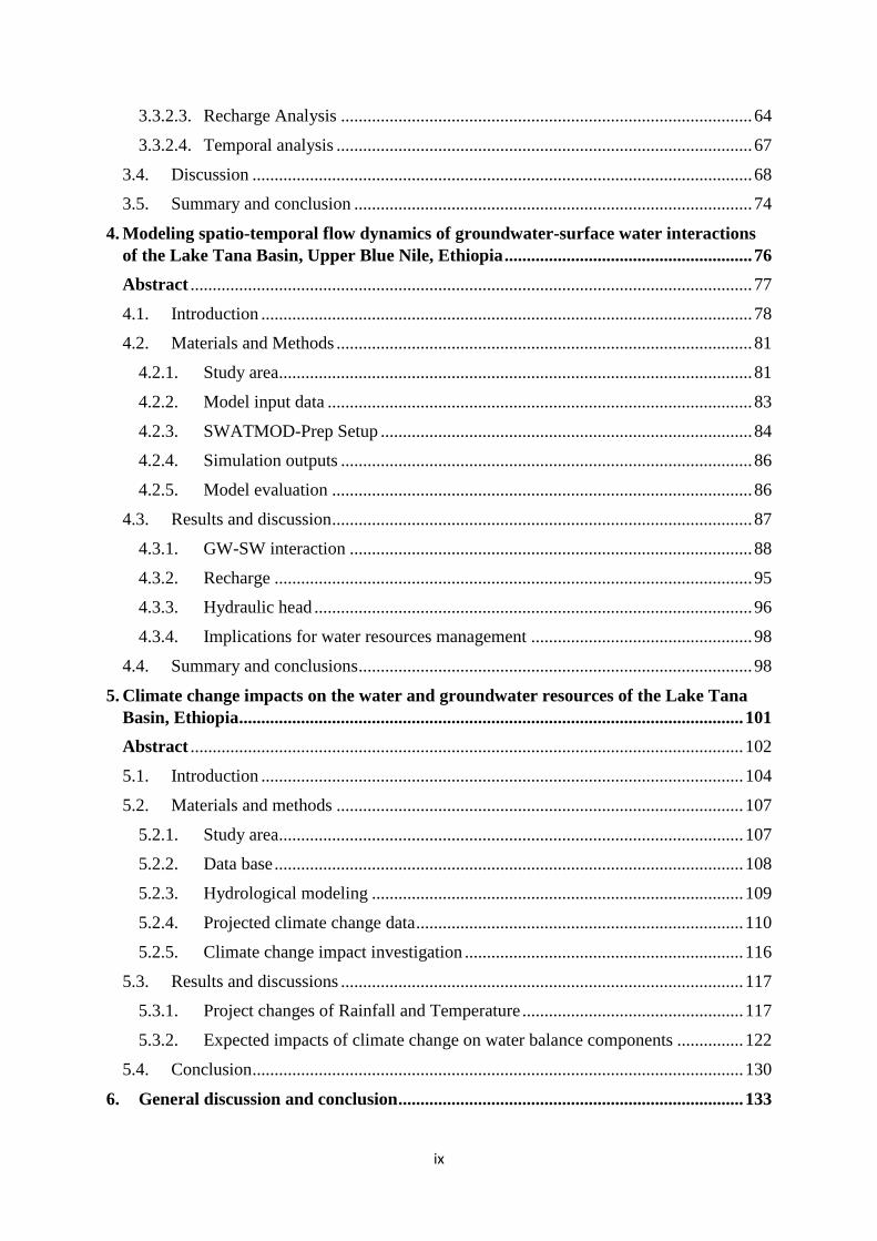
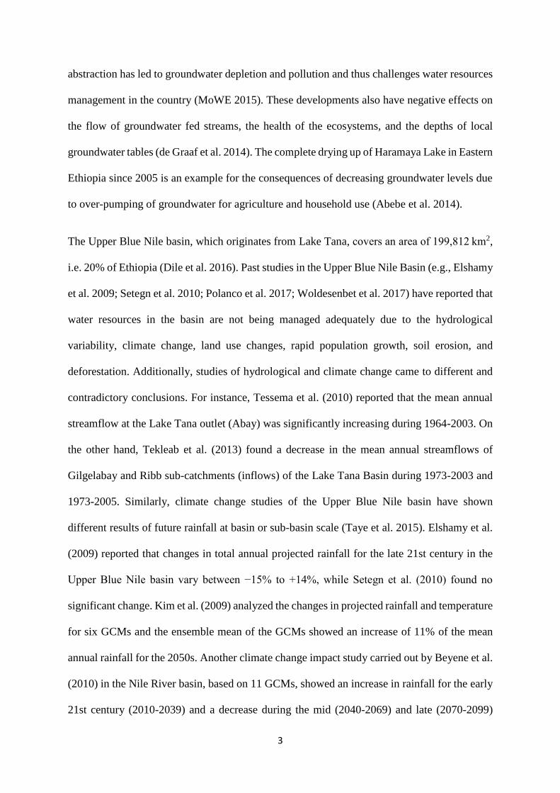
The Lake Tana basin (Figure 1) supports the livelihood of more than 3 million people, and it
is well known for its water resource potential. Being the sub-basin of Upper Blue Nile basin,
Lake Tana basin is dominated by intensive agriculture with a high impact on the basin
hydrologic regime and ecological condition (Setegn et al. 2010). Moreover, Lake Tana Basin
became a focus area of many scientific studies because of its national and international
importance. These include water balance analyses of different sub-catchments including the
lake (Derib 2013; Tegegne et al. 2013; Dessie et al. 2015), hydrological modeling with
emphasis on surface water (eg. Dessie et al. 2014; Worqlul et al. 2015; Polanco et al. 2017),
hydrometeorological trend analyses (e.g. Gebrehiwot et al. 2014; Mengistu and Lal 2014),
climate change impact studies (e.g. Koch and Cherie 2013; Teshome 2016), land use/cover
change impact on hydrologic responses (e.g. Gumindoga et al. 2014; Woldesenbet et al. 2017),
implications of water harvesting intensification on upstream–downstream ecosystem services
and water availability (e.g. Dile et al. 2016), and groundwater and hydrogeology (e.g. Yitbarek
et al. 2012; Awange et al. 2014).
5
Figure 1-1: Location Map of Lake Tana Basin with reference to Amhara reginal state and
Ethiopia
1.2. Analysis of hydrometeorological time series
The analysis of historical patterns of hydrometeorological variables is an integral part of water
resource development programs (Gebrehiwot et al. 2014). Good quality rainfall and streamflow
data are required for hydrological as well as climate change studies and can often be taken from
observation networks (Stahl et al. 2010). Hence, time series analysis of hydrometeorological
data is a crucial prerequisite for hydrological modelling studies. Statistical hydrology has
emerged as a powerful tool for analysing hydrologic time series of both surface water and
groundwater systems during the past three decades (Machiwal and Jha 2006). Trend detection,
test of homogeneity (stationarity), seasonality, and decadal tests are the most frequently used
statistical tests in hydrology. Gradual change over time which is consistent in direction
(monotonic) or an abrupt shift (breakpoint) at a specific point in time on time series records is
6
known as trend (Meals et al. 2011). A stationary or homogeneous time series is one whose
statistical properties such as mean, variance, autocorrelation, and other statistical properties are
all constant over time, otherwise it is called non-stationary. The existence of trends in hydro-
climatic variables such as rainfall, temperature, humidity, evapotranspiration, and streamflow
are an indication of climatic variability and climate change (Birsan et al. 2005; Rashid et al.
2015). Investigating the existence of trends is a widely recognized statistical approach to detect
non-stationarity in time series (Taye et al. 2015). Trend detection can be applied in all-time
series of hydrometeorological variables such as rainfall, temperature, humidity, wind speed,
and streamflow.
1.3. Hydrological modeling
Hydrological models are relevant tools to better land and water management practices (Palanco
et al. 2017). The use of physically based hydrologic models has been increasing over time
because of their capabilities to incorporate physical processes of the system. The Soil and
Water Assessment Tool (SWAT) model (Arnold et al. 1998, Arnold and Fohrer 2005) is one
of the most widely applied river basin-scale hydrologic model. Because of its adaptability for
both large and small scale catchments and continuous improvement, researchers in different
fields have identified SWAT as one of the most intricate, dependable, and computationally
efficient models (Neitsch et al. 2011; Palanco et al. 2017). The model is capable of simulating
spatially distributed water balance components based on hydrological response units (HRUs).
Likewise, application of the SWAT model in Ethiopian watersheds is expanding over time.
Among others, the following are a few case studies that applied SWAT as their modelling tool.
Setegn et al. (2009, 2011) used SWAT2005 to test its applicability in the Lake Tana Basin and
applied to evaluate the past and future water balance situation of the basin. With this study, the
authors concluded that SWAT model was capable to model the hydrologic al processes of the
Lake Tana basin. Their water balance results showed that actual ET accounts more than 60%
7
of the basin hydrologic processes, and the groundwater contribution to the streamflow varies
between 40% and 60%. Dile et al. (2013) used the SWAT model to study the effects of climate
change on hydrological responses of Gilgelabay catchment. According to this study, the
monthly mean volume of runoff the catchment tends to increase significantly (up to 135%) for
the mid and long-term of the 21st century. Dile et al. (2016) used SWAT2012 for their study
to investigate the implications of intensive water harvesting on upstream–downstream
ecosystem services in the Lake Tana basin. In these studies, they found that intensification of
water harvesting in the basin would increase low flows and decrease peak flows. They also
found a reduction in the amount of sediment yield that leave the catchment. Polanco et al.
(2017) applied SWAT model to investigate the effect of discretization on its performances in
the entire Upper Blue Nile Basin under. Their finds showed that increasing the number of sub-
basins would affect the magnitude of streamflow and other water balance components and the
authors suggested increasing the number of sub-basins is important to improve the
performances of SWAT model in the basin. Another hydrological assessment study by Desta
and Lemma (2017) in the Lake Ziway watershed, Rift valley, Ethiopia used SWAT as their
modelling tool, and their finds showed that the annual base flow is decreasing, while actual ET
is increasing over time. Overall, all studies proved that SWAT models is capable to simulate
the hydrological processes in Ethiopia as a whole and in Upper Nile basin in particular.
However, all of studies considered the water balance components at the outlets of the study
catchments ignoring spatial distributions of water balance components. In addition to this, the
seasonal and spatial variability of the hydrological components under different vegetation
cover condition are missed.
1.4. Groundwater dynamics and climate change
Aquifers are the largest storage of global freshwater: more than two billion people rely on
groundwater (Cuthbert et al. 2019). Groundwater (GW) accounts for one third of all freshwater
8
withdrawals of the world, supplying an estimated 36%, 42% and 27% of the water for domestic,
agricultural and industrial purposes, respectively (Taylor et al. 2013). Although GW is
vulnerable to depletion, it is being consumed faster than it is being naturally replenished
(Rodell et al. 2009; Sutanudjaja et al. 2011). The rapid population growth, expansion of
irrigation agriculture, and economic development globally increased the water demand, and
leads to water stress in several parts of the world (Wada et al. 2010). Groundwater levels and
fluxes are controlled by a dynamic interplay between recharge and discharge, with a variety of
controls and feedback loops from climate, soils, geology, land cover and human abstraction
(Cuthbert et al. 2019). According to Abbaspour et al. (2015), the quality and quantity of GW
in Europe are under heavy pressure and water levels have decreased. Compared to surface
water, groundwater responds more slowly to changes in meteorological conditions (Bovolo et
al. 2009). As a result, the laws governing groundwater rights are still static even in developed
countries (Rodell et al. 2009). This aggravates overexploitation of GW worldwide and very
pronouncedly in arid regions (Hashemi et al. 2015). Higher standards of living, demographic
changes, land and water use policies, and other external forces are increasing the pressure on
groundwater resources. In Ethiopia, 80% the national water demand is covered from
groundwater source (Kebede 2012). The total annual aquifer recharge is estimated to be more
than 30 billion cubic meter (Berhanu et al. 2014; Kebede 2010). Due to the infancy institutes
and research capabilities in the country, our knowledge about the groundwater recharge,
groundwater-surface water connection, and aquifer properties is limited (Berhanu et al. 2014).
Therefore, combined use of groundwater (GW) and surface water (SW), understanding
the groundwater (GW) - surface water (SW) interaction, and investigating the effect of
climate change on GW are urgent issues that need to be addressed.
So far, a number of models are developed to study the interaction between GW and SW.
According to (Zhou and Li 2011), 1966 was a year when numerical models were applied for
9
the first time to simulate steady state regional flow patterns of hypothetical aquifer systems.
Since then, numerous physically based models were evolved (eg. MODFLOW, Harbaugh et
al. 2000) and applied to improve understanding of process dynamics. Interests of developing
and using coupled land surface and subsurface models are growing. Coupling of MODFLOW
with SWAT model is a recent advancement. Bailey et al. (2016) developed the coupled SWAT-
MODFLOW model that was upgraded later into the graphical user interface model
SWATMOD-Prep (Bailey et al. 2017). Ehtiat et al. (2018) integrated SWAT, MODFLOW,
and MT3DMS to investigate how SW conditions affect the quality of the GW system in a non-
coastal aquifer. Similarly, Park et al. (2019) developed a QGIS-based graphical user interface
SWAT-MODFLOW model for Middle Bosque River Watershed in central Texas. These
advancements of coupled model development are derived due to the deficiencies associated
with surface water and groundwater models. Although SWAT model has wide range of
application history, it has a limitation to simulate groundwater dynamics below threshold depth
of 6m (Neitsch et al., 2011; Guzman et al. 2015; Shao et al. 2019). It uses the hydrologic
response units (HRUs) as its smallest spatial computation unit where there is no exchange of
water between different HRUs (Chunn et al. 2019), and the HRUs are lack of geolocation that
result spatial disconnection (Guzman et al. 2015; Bailey et al. 2016). Additionally, SWAT has
a limitation to capture groundwater dominated low flows (Pfannerstill et al. 2014). The
MODFLOW also has its own limitation to simulate the surface hydrologic processes because
its subroutines are designed to simulate flow processes occurring in the saturated zone such as
GW recharge, GW discharge, and pumping (Harbaugh 2005). Thus, application of coupled
model like SWATMODFLOW (Bailey et al. 2016, Bailey et al. 2017) will provide additional
information such as volumetric exchange rates between the surface water and groundwater,
groundwater discharge and stream seepage areas, deep percolation to the aquifer, and
distributed groundwater head. Thus, use of such coupled hydrological model is important in
10
regions like Ethiopia where there is a knowledge gap about the groundwater-surface water
interaction.
Uncertainties related to water resources management are growing due to the effect of climate
change (Abbaspour et al. 2015). For this reason, a lot of research efforts are advancing overtime
to understand the influence of climate change on water resources system. For example, Givati
et al. (2019) studied the impact of climate change on streamflow of at the upper Jordan River
based on an ensemble projected regional climate data. In this study, the authors used projected
rainfall and temperature datasets of nineteen regional climate models (RCMs) from the
CORDEX project for RCP4.5 and RCP8.5 scenarios. Marx et al. (2018) studied how global
warming alter the low flows in Europe based on multi-model ensemble under three
concentration pathways (RCP2.6, RCP6.0, and RCP8.5). Past climate change impact studies
primarily focused on surface water, and only a few of them addressed the effect of climate
change on groundwater (Goderniaux et al. 2009; Kidmose et al. 2013). However, there are
recent advancement towards investigating the impact of climate change on groundwater (e.g.,
Cuthbert et al. 2019a studied the global patterns and dynamics of climate–groundwater
interactions; Cuthbert et al. 2019b investigated resilience of groundwater to climate variability
in in sub-Saharan Africa). Chunn et al. (2019) studied the impacts of climate change and water
withdrawal on the GW-SW interactions in West-Central Alberta using the integrated SWAT-
MODFLOW model. The potential impact of climate change on GW varies both temporally and
spatially. Both a decrease and increase of groundwater levels are reported. Ali et al. (2012)
reported that the GW system in the south-western Australia was less affected by the future drier
climate than the surface water system, but projected water tables are expected to decline in all
areas under a drier climate where perennial vegetation was present and able to intercept
recharge or use groundwater directly. An increase of the GW table is expected for future
climate conditions in irrigation-dominated areas in the Oliver region of the south Okanagan,
11
British Columbia (BC), Canada (Toews and Allen 2009). A climate change impact study by
Döll (2009) revealed an increase of groundwater recharge in northern latitudes, while 30–70%
decrease is expected in semi-arid zones, including the Mediterranean, north-eastern Brazil and
south-western Africa between 1961–1990 and 2041–2070. A recent study conducted by
Cuthbert et al. (2019) in sub-Saharan Africa indicated that the multiyear continuous GW levels
decline in Tanzania, Namibia, and South Africa, while long-term rising trends were reported
for Niger. Another climate change impact study carried out in the Ethiopian Tekeze basin
(Kahsay et al. 2018) based on the Coordinated Regional Climate Downscaling Experiment
(CORDEX) Africa datasets for Representative Concentration Pathways (RCPs) of RCP 2.6
and RCP 4.5 scenarios showed decreases in the projected GW recharge by 3.4% for RCP 2.6
and 1.3% for RCP 4.5, respectively. Overall, study results on the effect of climate change on
GW show that the magnitude and scale of influences vary from one geographic location to
another, and very few studies are available for Africa in general and Ethiopia in particular. This
indicates that the hydrological processes controlling groundwater recharge and
sustainability, and sensitivity to climate change in Africa are poorly understood and cause
high uncertainties for future water resources management and planning (Cuthbert et al.
2019b). Hence, more research efforts are required with regard to climate change impact on GW
to minimize the uncertainties related to future water management and planning in Africa.
1.5. Statement of the problem and research questions
The major challenge of Ethiopian water resources management is the very high water
variability in combination with marked rainfall seasonality (World Bank 2006). Moreover,
hydrologic processes in the Lake Tana basin are not yet fully understood due to its complex
biophysical processes and scarcity of hydrometeorological data (Leggesse and Beyene 2017).
Consequently, this is dissertation was designed to answer multiple research questions that are
related to water resources of the Lake Tana basin based on observed hydrological and climate
12
time series data during the last half-century, and simulated outputs from a physically based
hydrologic models for current and future time periods.
Tesemma et al. (2010) and Tekleab et al. (2013) studied the trends of hydrometeorological
variables within the upper Blue Nile basin. They used the Mann-Kendall, Pettitt, and Sen’s t-
tests for trend analysis and found a significant increase in discharge during the rainy season
(June to September) at Bahir Dar, Kessie, and El Diem gauging stations, whereas seasonal and
annual basin-wide average rainfall trends were not significant. On the one hand, Mengistu et
al. (2014) reported an increasing trend on the annual total rainfall of the upper Blue Nile basin
for the years between 1980 and 2010 (35mm per decade), but the change was not statistically
significant. On the other hand, the basin-wide annual rainfall of upper Blue Nile basin showed
an insignificant decreasing trend during 1954 to 2004 (Tabari et al. 2015). Gebrehiwot et al.
(2014) investigated statistical changes on the long-term hydrology of catchments within upper
Blue Nile and found that the hydrological regime of the upper Blue Nile Basin during 1960–
2004 was stable. However, there the low flow decreased in some watersheds and increased in
others. Generally speaking, past hydrometeorological trend studies conducted so far in Ethiopia
are not conclusive and some are only conducted at the macro scale (Asfaw et al. 2018); findings
are not in agreement. This implies that additional research effort is needed to advance our
understanding of hydrometeorological condition in the country and in Lake Tana basin. For
this reason, the first research question of this PhD dissertations is formulated as follows:
were there significant long-term changes (1960-2015) in rainfall, streamflow, and lake
outflow time series observable in the Lake Tana basin?
The Lake Tana basin is known for its national and international importance. It has significant
national importance because the government of Ethiopia has identified it as a potential area for
irrigation and hydropower development, which are vital for food security and economic growth
in the country (Tegegne et al. 2017). Similarly, the Lake Tana basin is of international
13
importance as it is a headwater source of the Nile River and an area of high biodiversity (Setegn
et. al. 2010). As a consequence, several hydrological models from simple conceptual to more
advanced physically and semi-physically based hydrological models have been applied to
understand hydrological processes and the water balance of the Lake Tana basin (Dile et al.
2018). However, most of the past hydrological studies focus on the water balance at basin
outlets and lack detailed mapping of water balance components on a spatial basis. In addition,
the hydrologic studies do not investigate the hydrologic mass balance in relation to vegetation
types (van Griensven et al. 2012). Although the SWAT model was used to investigate the effect
of land use change on the hydrology of the basin, none of the papers explicitly addressed the
specific effects of crops on the water fluxes. Here, the second key purpose of this PhD
dissertation is to answer the following research question:
how do the major water balance components vary on spatial and seasonal basis under
different agricultural crops and land use/cover classes?
According to the Ethiopian government growth and transformation plan, agriculture irrigated
from GW sources is expected to cover 2 million hectares by 2020 (Kebede 2012). Due to its
proximity to the point of demand, GW provides 90% of the domestic water supply, 95% of the
industrial use, and a small proportion of irrigation water demand. In general, 80% of the total
national water supply comes from GW (Kebede 2018). Previous hydrological studies focused
on the surface water use and hydrologic balance and do not adequately address issues of GW,
particularly in the context of combining SW–GW models in the Lake Tana Basin. Dile et al.
(2018) reviewed research in the upper Blue Nile basin. According to this review, application
of integrated hydrologic models is missing, as most studies have focused on single model
applications to estimate a single output such as streamflow or sediment loss at the basin outlet.
Consequently, the authors recommended that future research should focus on the application
14
of coupled models to predict multiple outcomes across multiple spatial and temporal scales in
the basin. Additionally, Chebud and Melesse (2009), who applied a numerical model to
investigate the groundwater flow system in the Gumara catchment, identified a research gap
on the spatial and temporal distribution of percolation in the Gumara catchment in particular,
and in Lake Tana Basin in general. A climate change impact study carried out by Taye et al.
(2015) in the Lake Tana basin reported that low flows are expected to decline by up to -61%
under the A1B and B1 emission scenarios for 2050s. Consequently, it is assumed that more
GW will be used to overcome the freshwater constraint in Ethiopia in general and in the Lake
Tana Basin in particular. From this, we can understand that demand of groundwater for
agricultural, domestic, and industrial uses in the future are expected to increase. However, our
knowledge about the GW-SW flow dynamics on the spatio-temporal basis for the current and
future condition is limited. Hence, answering the following two key research questions will
enhance our understanding about the GW-SW flow dynamics and future water availability in
the Lake Tana Basin.
Do the groundwater and surface water systems interact with each other and how
does the behaviour of GW-SW interaction vary in space and time?
How will future climate change affect the major water balance components of
the Lake Tana basin?
1.6. Thesis structure
The PhD thesis is divided into six chapters. The first chapter is the general introduction that
includes background information, state of the art and motivation of the research that explains
the derived research questions. The second chapter deals with time series analysis of the rainfall
and streamflow data of the past half century. In the third chapter, hydrologic changes under the
influence of different agricultural crops are addressed. The fifth chapter focuses on the
hydrologic flow dynamics of groundwater and surface water conditions in the Lake Tana Basin.

15
Anticipated changes of hydrology due to climate change are discussed in chapter five. The last
chapter focusses on the general discussion and conclusion of the overall outcomes of the
dissertation.
16
2. Statistical analysis of rainfall and streamflow time series in the Lake
Tana Basin, Ethiopia
Tibebe Belete Tigabu, Georg Hörmann, Paul D. Wagner and Nicola Fohrer
Department of Hydrology and Water Resources Management, Institute for Natural Resource
Conservation, Kiel University, D-24118 Kiel, Germany
Address to correspondence author: Tibebe Tigabu, Department of Hydrology and Water
Resources Management, Institute of Natural Resource Conservation, CAU, D-24118 Kiel,
Germany, E-mail: [email protected]
Journal of Water and Climate Change jwc2018008, https://doi.org/10.2166/wcc.2018.008.
Submitted: 16 December 2017– Accepted: 30 July 2018-printed March 2020, 11(1), pp.258-
273.
17
Abstract
This research focuses on the statistical analyses of hydrometeorological time series in the basin
of Lake Tana, the largest freshwater lake in Ethiopia. We used autocorrelation, cross-
correlation, Mann-Kendall, and Tukey multiple mean comparison tests to understand the
spatiotemporal variation of the hydrometeorological data in the period from 1960 to 2015. Our
results show that mean annual streamflow and the lake water level are varying significantly
from decade to decade whereas the mean annual rainfall variation is not significant. The
decadal mean of the lake outflow and the lake water level decreased between the 1990s and
2000s by 11.34 m3/s and 0.35 m, respectively. The autocorrelation for both rainfall and
streamflow were significantly different from zero indicating that the sample data are non-
random. Changes in streamflow and lake water level are linked to land use changes.
Improvements in agricultural water management could contribute to mitigate the decreasing
trends.
Keywords: hydrometeorology; autocorrelation; cross-correlation; Tukey’s test;
temporal variation.
18
2.1. Introduction
Management and analysis of time series data are integral parts of hydrological and climate
studies. Good quality data are required for climate change detection as well as for hydrological
studies and can often be taken from observation networks (Stahl et al. 2010). Data can be
accessed in different formats from different organizations and should be managed properly.
There are a number of tools for data management, analysis and interpretation e.g. SPSS, R and
Matlab which are capable of accessing data from many different sources and a smaller number
of systems capable of handling data management, analysis and interpretation (Horsburgh and
Reeder 2014). Different kinds of data analysis methods can be chosen for different research
objectives. Time series analysis of rainfall and streamflow is crucial as it is a prerequisite for
further using the data in e.g. hydrological modelling studies. A time series is defined as a
sequence formed by the values of a variable at increasing points in time that may be composed
of a random element and a non-random element (Matalas 1967). It is said to be random if the
values of the time series are independent of each other, otherwise it is non-random. A non-
randomly distributed sequence repeats some of the information contained in previous values.
The nature of hydrolometeorological data can be investigated by testing their randomness,
trend and association with other variables such as biophysical and socio-economic variables.
For instance, the interaction of hydrological variables with land use changes has been studied
by Wagner and Waske (2016) and Wagner et al. (2016). Persistence of a trend and its
magnitude in hydrological time series data were studied by different scholars (e.g. Thomas &
Pool 2006, Stahl et al. 2010, Hawtree et al. 2017, Wagner et al. 2018). A number of
hydrological studies were carried out in Ethiopia in general, in Lake Tana Basin in particular
(Setegn et al. 2008; Alemayehu et al. 2009; Alemayehu et al. 2010; Dargahi and Setegn 2011;
Koch and Cherie 2013; Gebremicael et al. 2013; Mehari, K.A. et al. 2014; Dessie et al. 2015;
Woldesenbet et al. 2017). For instance, Woldesenbet et al. (2017) studied the impact of land
19
use land cover change on streamflow of Tana and Beles sub-basins in Ethiopia. This research
revealed that the average annual water yield, the average annual baseflow and average annual
basin percolation decreased gradually, to the contrary the average annual surface runoff
increased. These changes are associated with expansion of cultivation land and the shrinkage
in woody shrub from 1986 to 2010. Koch and Cherie (2013) studied the impact of future
climate change on hydrology and water resources management of the whole Upper Blue Nile
Basin. Streamflow records over the time period 1970-2000 of Abay River at Eldiem gauging
station close to the Ethio-Sudan border were analysed using Mann-Kendall and the seasonal
Mann-Kendall test and the result showed a significantly increase trend (Koch and Cherie 2013).
Although many research studies were done on various hydrological and environmental issues
in the Blue Nile basin, very few of them were focused on long-term trends of
hydrometeorological variables at catchment level (Tekleab et al. 2013). Furthermore, there
were conflicting results on the trends of hydrometeorological time series in the Blue Nile basin.
For instance, Tessema et al. (2010) reported that the mean annual streamflow at the Lake Tana
outlet (Abay) was significantly increasing during 1964-2003. On the other hand, Tekleab et al.
(2013) found a decrease of the mean annual streamflows of Gilgleabay and Ribb sub-
catchments (inflows) of the Lake Tana Basin during 1973-2005/2003. This indicates that
analyses on one long term time series alone might not be sufficient to understand
hydrometeorological variabilities. Moreover, most of the hydrometeorological variability and
trend analysis studies were carried out using Mann-Kendall (MK) and Pettitt tests as the only
methods of investigations. On top of that, hydrometereological trend analysis studies conducted
so far in Ethiopia are not conclusive and some are conducted at macro scale, underlining the
need for further research (Asfaw et al. 2018). As Ethiopia is strongly dependent on agriculture
with a highly variable hydrology, its agricultural yield is frequently affected by droughts and
famines. The United Nations Children’s Fund (UNICEF) reported that the 2015-2017 drought
20
caused by El-Nino effect is one of the worst droughts in decades (UNICEF 2016).
Consequently, improved understanding of the patterns of historical observed
hydrometeorological time series on the local scale using different time spans is crucial for water
use and management. Since the study area is highly dynamic with respect to hydrology and
most of the previous studies were carried out on the macro-scale, attention should be given to
hydrometeorological changes on the local scale. Therefore, this study aims at conducting a
thorough analyses of the temporal and spatial variation of long-term rainfall, streamflow and
lake water level in the Lake Tana Basins over the period (from 1960 to 2015) on decadal,
annual, seasonal, and daily time scales. To this end multiple statistical methods such as Tukey
multiple mean comparison tests, autocorrelation, cross-correlation and MK test are used to
characterize the decadal and seasonal changes, dependency of events on the adjacent ones with
respect to time, response of streamflow to rainfall events and existence of trends. Accordingly,
the research questions were the following:
Are the rainfall/ streamflow events related to their preceding ones?
Are the time series data random or non-random?
Are rainfall and streamflow events cross-correlated?
Do decadal, annual and seasonal rainfall, streamflow and lake water levels show
significant changes over time?
2.2. Materials and Methods
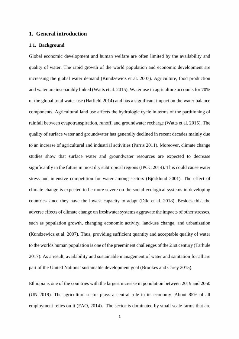
2.2.1. General overview of the study area
Lake Tana is the largest freshwater lake in Ethiopia and the third largest in the Nile Basin. The
catchment area of the lake at its outlet is 15,321 km2. About 20% of the catchment area is
covered by Lake Tana (Alemayehu et al. 2010, Kebede et al. 2006). The catchment is
approximately 84 km long, 66 km wide and is located in the country's north-west highlands.
21
Its topography is very diverse with an altitude ranging from 1322 m to 4111 m above sea level
(m.a.s.l.). The lake has a surface area of 3,156 km2 and extends between 10.95°N to 12.78°N
latitude and from 36.89°E to 38.25°E longitude at an average altitude of 1,786 (m.a.s.l.),
(Tegegne et al. 2013).The lake is shallow with a maximum depth of 15 m and characterized by
a steep slope at the borders and by a flat bottom (Kebede et al. 2006). Lake Tana is the source
of the Blue Nile River (McCartney et al. 2010). It contains about 50% of the country’s fresh
water. More than 40 rivers and streams flow into Lake Tana, but 93% of the water comes just
from four major rivers: Gilgelabay, Gumara, Ribb and Megech (Setegn et al. 2008; Alemayehu
et al. 2010). The mean annual inflow is estimated to be 158 m3/s (Alemayehu et al. 2010). The
only surface outflow from the lake is the Blue Nile (Abay) River with an annual flow volume
of 4 billion m3 measured at Bahir Dar gauge station (lake outlet in Fig. 1).
Rainfall records in the basin show strong spatial and temporal variability as the basin is
influenced by the inter-tropical convergent zone (ITCZ) and a heterogeneous topographic
nature. The position of the ITCZ is the most dominant factor that controls the amount of
summer rainfall in the basin. In the Lake Tana basin, rainfall has high seasonal variability. July,
August & September are wet months with the highest amounts of rainfall as the ITCZ position
is in the northern hemisphere. June and October are transition months of wet and dry seasons.
November, December, January, February, and March belong to the dry season. April and May
are months with little rainfall. A similar classification applies to the West Sahel region (Lucio
et al. 2012). There is also high spatial variability of annual, seasonal and monthly rainfall
amounts in the study area because of small changes of the location of the ITCZ (Gleixner et al.
2016; Woldesenbet et al. 2017). Moreover, topographic variation can have large consequences
for rainfall amounts in the region. The amount of annual rainfall is directly related to elevation
above mean sea level; high rainfall is corresponding to the highlands, whereas low rainfall is
measured in the lowlands (Fig. 5).
22
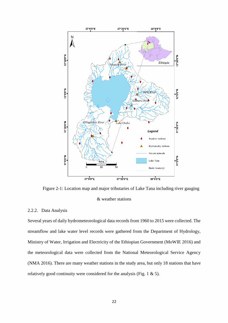
Figure 2-1: Location map and major tributaries of Lake Tana including river gauging
& weather stations
2.2.2. Data Analysis
Several years of daily hydrometeorological data records from 1960 to 2015 were collected. The
streamflow and lake water level records were gathered from the Department of Hydrology,
Ministry of Water, Irrigation and Electricity of the Ethiopian Government (MoWIE 2016) and
the meteorological data were collected from the National Meteorological Service Agency
(NMA 2016). There are many weather stations in the study area, but only 18 stations that have
relatively good continuity were considered for the analysis (Fig. 1 & 5).
23
2.2.2.1.Statistical Methods
For this study, basic statistical analysis techniques including the Tukey’s multiple mean
comparisons, a nonparametric Kendall tau and seasonal Mann-Kendal tests as well as auto-
and cross-correlation analyses were used. These methods were chosen to understand the
variability of the hydrometeorological data over time as well as to characterize and detect the
relation between the hydrometeorological variables.
Tukey’s (“honestly significant difference” or “HSD”): Tukey's multiple comparison test is a
useful statistical method that can be used to determine which means amongst a set of means
differ from the rest (Bates 2010). For the first time, Tukey’s HSD test was applied in the Lake
Tana Basin to understand the variability of mean values of river discharge and lake water level
on a decadal basis. Streamflows of Gilgelabay, Gumara, Ribb, Megech, outflow from the Lake
Tana, and the lake water level were considered. The decadal analyses of streamflows at the
aforementioned stations and the lake water level were made by partitioning the recorded data
into different decades to understand the change of annual mean values overtime. The time
series data were split into the following decadal groups: 1960-1979, 1980-1989, 1990-1999
and 2000-2014. In this case, the null hypothesis assumed was that the annual mean values of
streamflows and lake water level were time invariant (same for different decades) and the
alternative hypothesis was that annual mean values differed with time. The 5% level of
significance was considered in all of these analyses. The anova and TukeyHSD functions
available in the base package of R were used to calculate the statistical values (R Core Team
2017).
Autocorrelation: Autocorrelation analysis provide information about persistence of a variable
by calculating the linear dependency of successive values over a given period. Mangin (1984)
first applied autocorrelation to karstic systems in the Pyrenees, France, to measure the
persistence of a signal in the series (Duvert et al. 2015). It is also commonly used to determine
24
if the data series is random or non-random (e.g. Matalas 1967; Modarres et al. 2007; Gautam
et al. 2010; Duvert et al. 2015). Autocorrelation coefficients of the rainfall and streamflow
events were calculated using equation (1) (Duvert et al. 2015). Furthermore, following to
(Matalas 1967), who refer to the Anderson (1942) for the test of significance of the
autocorrelation coefficient (acf) to a given probability level was tested based on equation (2).
𝑟𝑘 =1
𝑁∑ (𝑥𝑖−�̅�)𝑁−𝑘
𝑖=1 (𝑥𝑖+𝑘−�̅�)
𝛿2 =∑ (𝑥𝑖−�̅�)𝑁−𝑘
𝑖=1 (𝑥𝑖+𝑘−�̅�)
∑ (𝑥𝑖−�̅�)2𝑁𝑖=1
(1)
�̃�k =−1 ± 𝑡𝛼(√𝑁−k−1)
𝑁 − k (2)
where rk is the acf at lag k, �̅�, is arithmetic mean of the observation, tα is the standard normal
variate corresponding to a probability level α, �̃�1 is the upper and lower bounds and N is the
series length. The rk value calculated by equation (1) could be compared with the corresponding
value calculated using equations 2 for significance test. If the value calculated on equation 1 is
greater than values on equations 2, the rk seems to be significantly different from zero and the
sample observations are dependent on their preceding events at a given time lag k (Matalas
1967). Therefore, the null hypothesis (Ho) and alternative hypotheses (Ha) tests of this study
were the following:
Ho: events of the daily rainfall, streamflow and lake water level time series were not dependent
on their preceding events at time lag -k. In other words the autocorrelation coefficient at lag k
is not beyond or below the upper and lower bounds and the data were random. The alternative
assumption considered was the reverse one i.e. events of the daily rainfall and streamflow time
series were dependent to their preceding events at time lag k. In other words the autocorrelation
coefficient at lag k is out of the upper and lower bounds and the data were non-random.
Cross-Correlation: Cross-correlation is the correlation between two time series shifted
relatively in time. The method has been widely applied in diverse fields (Chenhua 2015).

25
Lagged correlation is important in studying the relationship between time series for two
reasons. First, one series may have a delayed response to the other series, or perhaps a delayed
response to a common stimulus that affects both series. Second, the response of one series to
the other series or an outside stimulus may be “smeared” in time, such that a stimulus restricted
to one observation causes a response at multiple observations. Detailed mathematical equations
are explained in (Duvert et al. 2015). Here we used cross-correlation of rainfall versus
streamflow.
Autocorrelations are symmetrical functions (value at lag k equals value at lag -k). In contrast,
the cross-correlations are asymmetrical functions. The cross-correlation function is described
in terms of “lead” and “lag” relationships. Equation (3) applies to yt shifted forward relative to
xt. With this direction of shift, xt is said to be “lead” yt. This is equivalent to saying that yt
“lags” xt. A negative value for k in equation (3) is a correlation between the x-variable at a time
before t and the y-variable at time t. For instance, if k=-1, the cc value would give the
correlation between xt-1 and yt (Chatfield 2004).
∑ (𝑥𝑖−�̅�)(𝑦𝑖+𝑘−�̅�)𝑁−𝑘𝑖=1
√∑ (𝑥𝑖−�̅�)2 ∑ (𝑦𝑖=1−�̅�)2𝑁𝑖=1
𝑁𝑖=1
[𝑘 = 0 ± 1, ±2, … , ±(𝑁 − 1)] (3)
where N is the series length, �̅� and 𝑦 ̅are the sample means, and k is the lag.
Pairwise cross-correlations of streamflow with the corresponding regional rainfall of each sub
basin were carried out. Cross-correlation (cc) tests were carried out for rainfall versus
streamflow based on the following null and alternative hypotheses tests stated as follows:
Ho: the daily streamflow and catchment rainfall time series are not correlated significantly or
the correlation coefficients at time lag k between daily streamflow and rainfall is not
significantly different from zero.
26
Ha: the daily streamflow and catchment rainfall time series are correlated significantly or the
correlation coefficients at time lag k between daily streamflow and rainfall is significantly
different from zero.
Kendall tau and seasonal Mann-Kendall tests: The Kendall and seasonal Mann-Kendall tau
tests are nonparametric statistical tests used for detecting trends in time series data (Thomas
and Pool 2006). The tests were applied for rainfall, the lake water level and streamflow time
series under the following null (Ho) and alternative (Ha) hypotheses:
Ho: the streamflow, rainfall and lake water level time series data are showing neither an upward
nor a downward trend.
Ha: the streamflow, rainfall and lake water level time series data are showing either an upward
or a downward trend with significant change.
2.3. Results and discussion
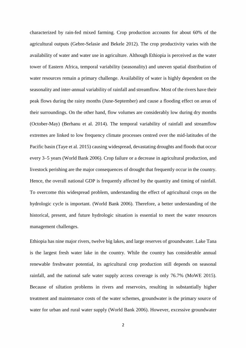
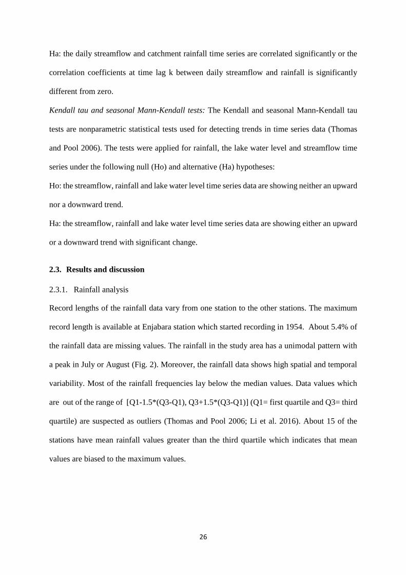
2.3.1. Rainfall analysis
Record lengths of the rainfall data vary from one station to the other stations. The maximum
record length is available at Enjabara station which started recording in 1954. About 5.4% of
the rainfall data are missing values. The rainfall in the study area has a unimodal pattern with
a peak in July or August (Fig. 2). Moreover, the rainfall data shows high spatial and temporal
variability. Most of the rainfall frequencies lay below the median values. Data values which
are out of the range of [Q1-1.5*(Q3-Q1), Q3+1.5*(Q3-Q1)] (Q1= first quartile and Q3= third
quartile) are suspected as outliers (Thomas and Pool 2006; Li et al. 2016). About 15 of the
stations have mean rainfall values greater than the third quartile which indicates that mean
values are biased to the maximum values.
27
Figure 2-2: A boxplot showing monthly rainfall plots of stations in Lake Tana Basin. The
dots indicate outliers outside the interquartile ranges.
28
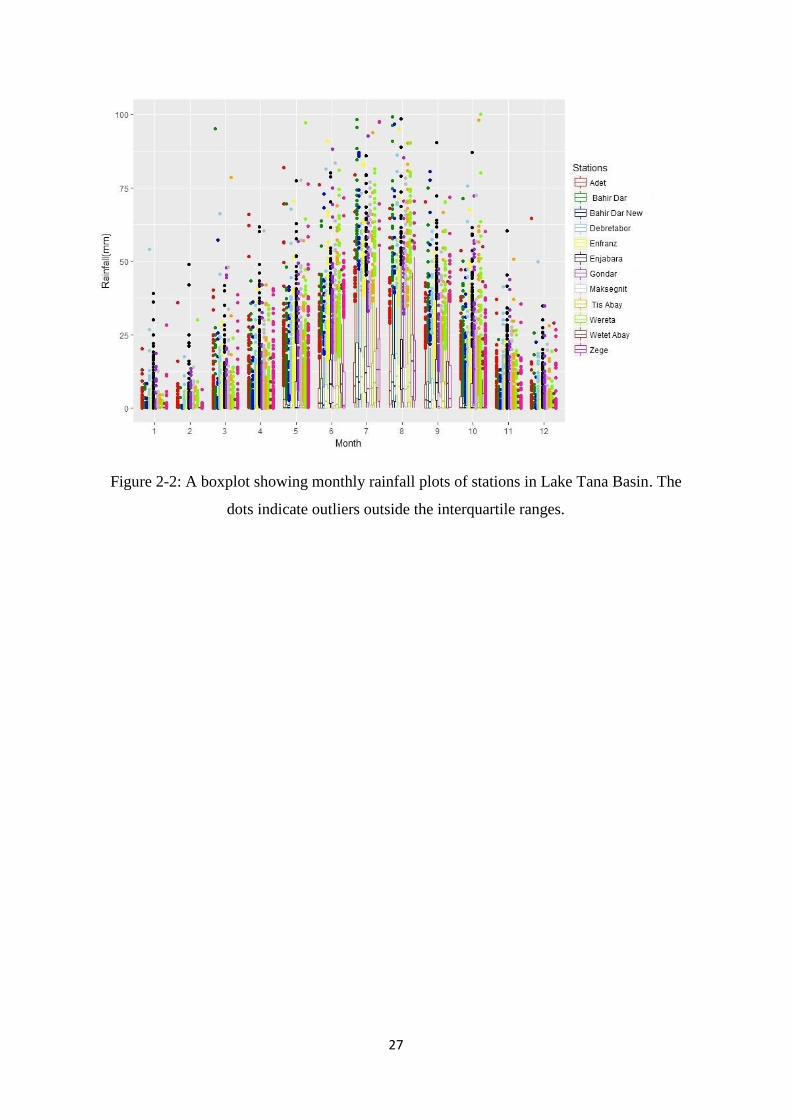
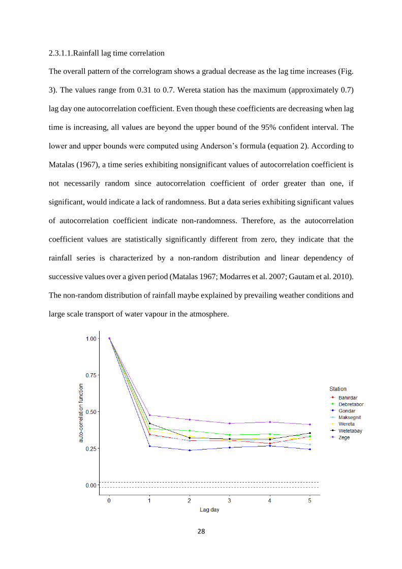
2.3.1.1.Rainfall lag time correlation
The overall pattern of the correlogram shows a gradual decrease as the lag time increases (Fig.
3). The values range from 0.31 to 0.7. Wereta station has the maximum (approximately 0.7)
lag day one autocorrelation coefficient. Even though these coefficients are decreasing when lag
time is increasing, all values are beyond the upper bound of the 95% confident interval. The
lower and upper bounds were computed using Anderson’s formula (equation 2). According to
Matalas (1967), a time series exhibiting nonsignificant values of autocorrelation coefficient is
not necessarily random since autocorrelation coefficient of order greater than one, if
significant, would indicate a lack of randomness. But a data series exhibiting significant values
of autocorrelation coefficient indicate non-randomness. Therefore, as the autocorrelation
coefficient values are statistically significantly different from zero, they indicate that the
rainfall series is characterized by a non-random distribution and linear dependency of
successive values over a given period (Matalas 1967; Modarres et al. 2007; Gautam et al. 2010).
The non-random distribution of rainfall maybe explained by prevailing weather conditions and
large scale transport of water vapour in the atmosphere.
29
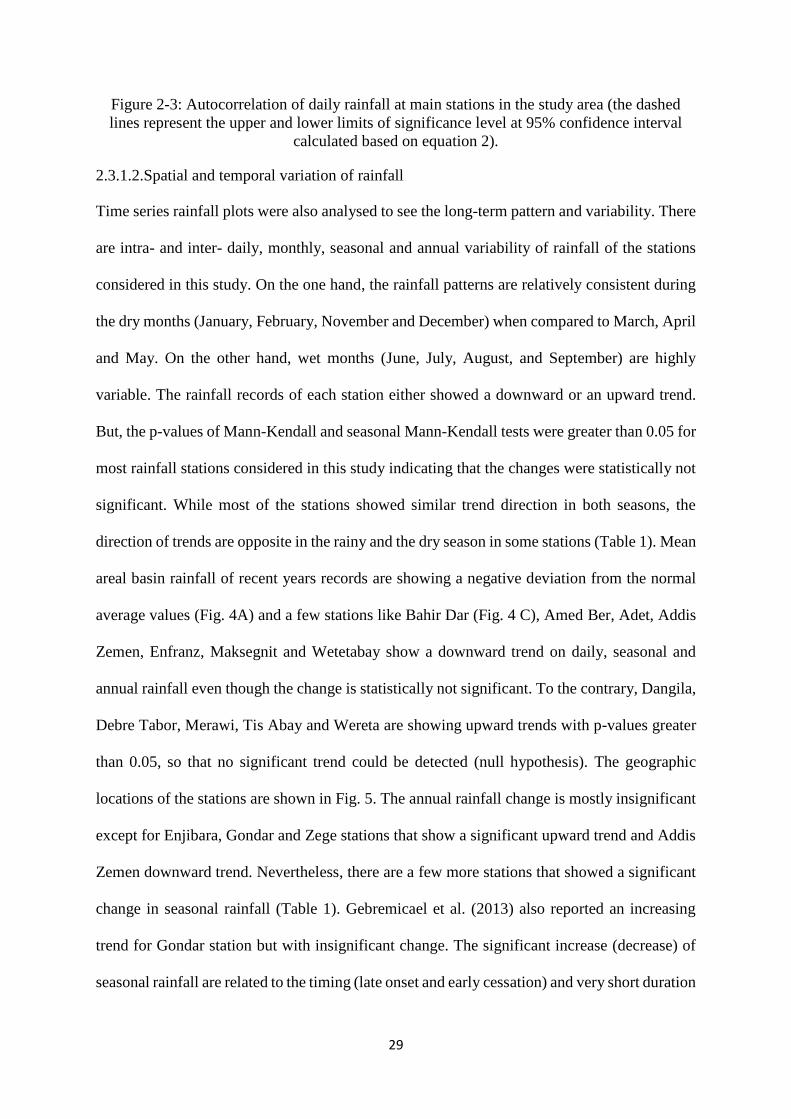
Figure 2-3: Autocorrelation of daily rainfall at main stations in the study area (the dashed
lines represent the upper and lower limits of significance level at 95% confidence interval
calculated based on equation 2).
2.3.1.2.Spatial and temporal variation of rainfall
Time series rainfall plots were also analysed to see the long-term pattern and variability. There
are intra- and inter- daily, monthly, seasonal and annual variability of rainfall of the stations
considered in this study. On the one hand, the rainfall patterns are relatively consistent during
the dry months (January, February, November and December) when compared to March, April
and May. On the other hand, wet months (June, July, August, and September) are highly
variable. The rainfall records of each station either showed a downward or an upward trend.
But, the p-values of Mann-Kendall and seasonal Mann-Kendall tests were greater than 0.05 for
most rainfall stations considered in this study indicating that the changes were statistically not
significant. While most of the stations showed similar trend direction in both seasons, the
direction of trends are opposite in the rainy and the dry season in some stations (Table 1). Mean
areal basin rainfall of recent years records are showing a negative deviation from the normal
average values (Fig. 4A) and a few stations like Bahir Dar (Fig. 4 C), Amed Ber, Adet, Addis
Zemen, Enfranz, Maksegnit and Wetetabay show a downward trend on daily, seasonal and
annual rainfall even though the change is statistically not significant. To the contrary, Dangila,
Debre Tabor, Merawi, Tis Abay and Wereta are showing upward trends with p-values greater
than 0.05, so that no significant trend could be detected (null hypothesis). The geographic
locations of the stations are shown in Fig. 5. The annual rainfall change is mostly insignificant
except for Enjibara, Gondar and Zege stations that show a significant upward trend and Addis
Zemen downward trend. Nevertheless, there are a few more stations that showed a significant
change in seasonal rainfall (Table 1). Gebremicael et al. (2013) also reported an increasing
trend for Gondar station but with insignificant change. The significant increase (decrease) of
seasonal rainfall are related to the timing (late onset and early cessation) and very short duration
30
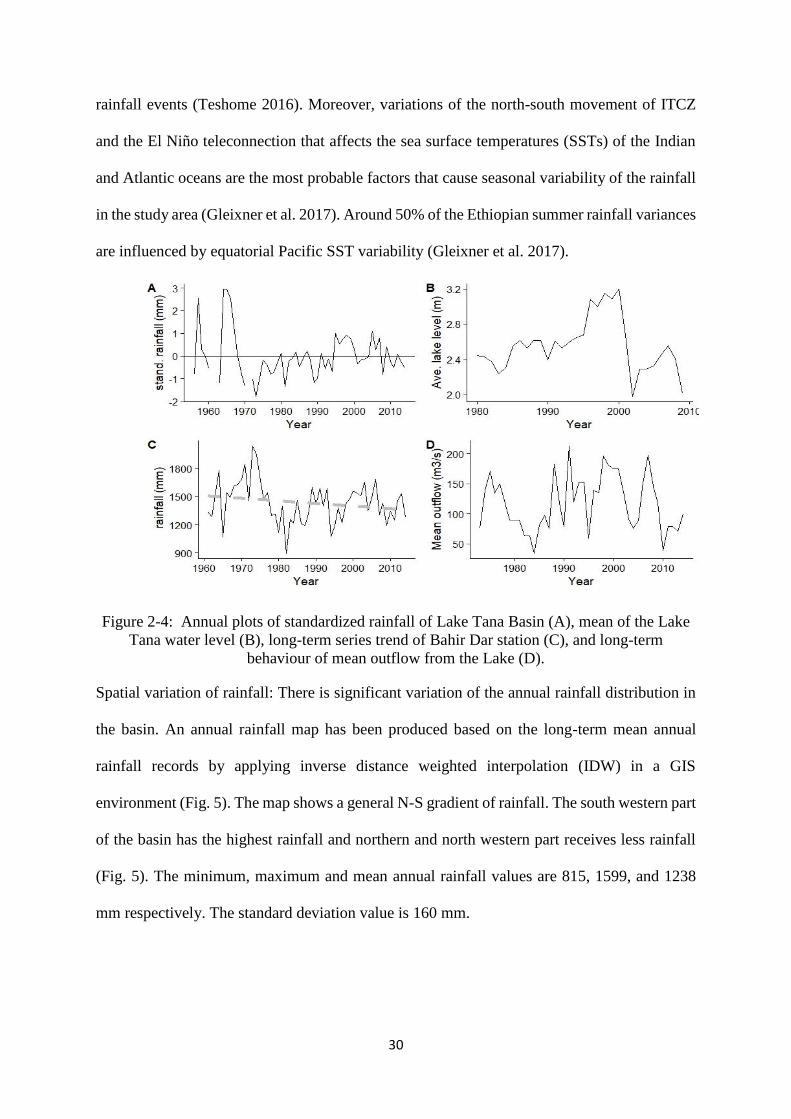
rainfall events (Teshome 2016). Moreover, variations of the north-south movement of ITCZ
and the El Niño teleconnection that affects the sea surface temperatures (SSTs) of the Indian
and Atlantic oceans are the most probable factors that cause seasonal variability of the rainfall
in the study area (Gleixner et al. 2017). Around 50% of the Ethiopian summer rainfall variances
are influenced by equatorial Pacific SST variability (Gleixner et al. 2017).
Figure 2-4: Annual plots of standardized rainfall of Lake Tana Basin (A), mean of the Lake
Tana water level (B), long-term series trend of Bahir Dar station (C), and long-term
behaviour of mean outflow from the Lake (D).
Spatial variation of rainfall: There is significant variation of the annual rainfall distribution in
the basin. An annual rainfall map has been produced based on the long-term mean annual
rainfall records by applying inverse distance weighted interpolation (IDW) in a GIS
environment (Fig. 5). The map shows a general N-S gradient of rainfall. The south western part
of the basin has the highest rainfall and northern and north western part receives less rainfall
(Fig. 5). The minimum, maximum and mean annual rainfall values are 815, 1599, and 1238
mm respectively. The standard deviation value is 160 mm.
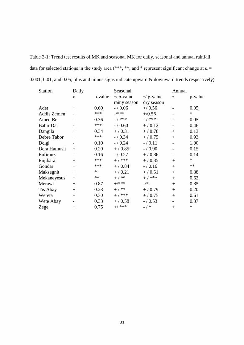
31
Table 2-1: Trend test results of MK and seasonal MK for daily, seasonal and annual rainfall
data for selected stations in the study area (***, **, and * represent significant change at α =
0.001, 0.01, and 0.05, plus and minus signs indicate upward & downward trends respectively)
Station Daily Seasonal Annual
τ p-value τ/ p-value
rainy season
τ/ p-value
dry season
τ p-value
Adet + 0.60 - / 0.06 +/ 0.56 - 0.05
Addis Zemen - *** -/*** +/0.56 - *
Amed Ber - 0.36 - / *** - / *** - 0.05
Bahir Dar - *** - / 0.60 + / 0.12 - 0.46
Dangila + 0.34 + / 0.31 + / 0.78 + 0.13
Debre Tabor + *** - / 0.34 + / 0.75 + 0.93
Delgi - 0.10 - / 0.24 - / 0.11 - 1.00
Dera Hamusit + 0.20 + / 0.85 - / 0.90 - 0.15
Enfiranz - 0.16 - / 0.27 + / 0.86 - 0.14
Enjibara + *** + / *** + / 0.85 + *
Gondar + *** + / 0.84 - / 0.16 + **
Maksegnit + * + / 0.21 + / 0.51 + 0.88
Mekaneyesus + ** + / ** + / *** + 0.62
Merawi + 0.87 +/*** -/* + 0.85
Tis Abay + 0.23 + / ** + / 0.79 + 0.20
Wereta + 0.30 + / *** + / 0.75 + 0.61
Wete Abay - 0.33 + / 0.58 - / 0.53 - 0.37
Zege + 0.75 +/ *** - / * + *
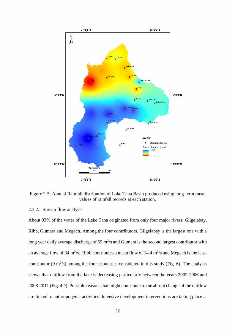
32
Figure 2-5: Annual Rainfall distribution of Lake Tana Basin produced using long-term mean
values of rainfall records at each station.
2.3.2. Stream flow analysis
About 93% of the water of the Lake Tana originated from only four major rivers: Gilgelabay,
Ribb, Gumara and Megech. Among the four contributors, Gilgelabay is the largest one with a
long year daily average discharge of 55 m3/s and Gumara is the second largest contributor with
an average flow of 34 m3/s. Ribb contributes a mean flow of 14.4 m3/s and Megech is the least
contributor (9 m3/s) among the four tributaries considered in this study (Fig. 6). The analysis
shows that outflow from the lake is decreasing particularly between the years 2002-2006 and
2008-2011 (Fig. 4D). Possible reasons that might contribute to the abrupt change of the outflow
are linked to anthropogenic activities. Intensive development interventions are taking place at
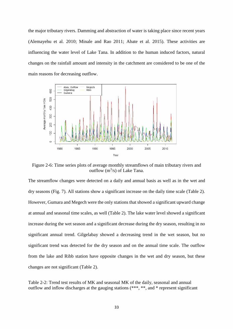
33
the major tributary rivers. Damming and abstraction of water is taking place since recent years
(Alemayehu et al. 2010; Minale and Rao 2011; Abate et al. 2015). These activities are
influencing the water level of Lake Tana. In addition to the human induced factors, natural
changes on the rainfall amount and intensity in the catchment are considered to be one of the
main reasons for decreasing outflow.
Figure 2-6: Time series plots of average monthly streamflows of main tributary rivers and
outflow (m3/s) of Lake Tana.
The streamflow changes were detected on a daily and annual basis as well as in the wet and
dry seasons (Fig. 7). All stations show a significant increase on the daily time scale (Table 2).
However, Gumara and Megech were the only stations that showed a significant upward change
at annual and seasonal time scales, as well (Table 2). The lake water level showed a significant
increase during the wet season and a significant decrease during the dry season, resulting in no
significant annual trend. Gilgelabay showed a decreasing trend in the wet season, but no
significant trend was detected for the dry season and on the annual time scale. The outflow
from the lake and Ribb station have opposite changes in the wet and dry season, but these
changes are not significant (Table 2).
Table 2-2: Trend test results of MK and seasonal MK of the daily, seasonal and annual
outflow and inflow discharges at the gauging stations (***, **, and * represent significant
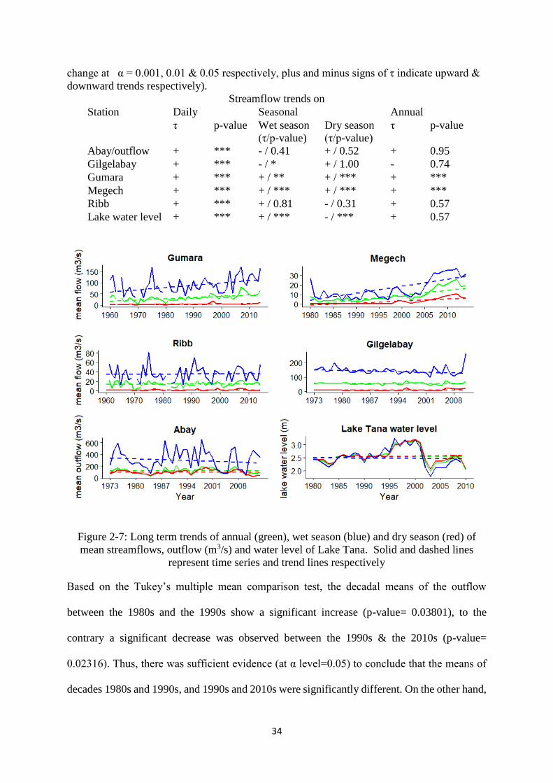
34
change at α = 0.001, 0.01 & 0.05 respectively, plus and minus signs of τ indicate upward &
downward trends respectively).
Streamflow trends on
Station Daily Seasonal Annual
τ p-value Wet season
(τ/p-value)
Dry season
(τ/p-value)
τ p-value
Abay/outflow + *** - / 0.41 + / 0.52 + 0.95
Gilgelabay + *** - / * + / 1.00 - 0.74
Gumara + *** + / ** + / *** + ***
Megech + *** + / *** + / *** + ***
Ribb + *** + / 0.81 - / 0.31 + 0.57
Lake water level + *** + / *** - / *** + 0.57
Figure 2-7: Long term trends of annual (green), wet season (blue) and dry season (red) of
mean streamflows, outflow (m3/s) and water level of Lake Tana. Solid and dashed lines
represent time series and trend lines respectively
Based on the Tukey’s multiple mean comparison test, the decadal means of the outflow
between the 1980s and the 1990s show a significant increase (p-value= 0.03801), to the
contrary a significant decrease was observed between the 1990s & the 2010s (p-value=
0.02316). Thus, there was sufficient evidence (at α level=0.05) to conclude that the means of
decades 1980s and 1990s, and 1990s and 2010s were significantly different. On the other hand,
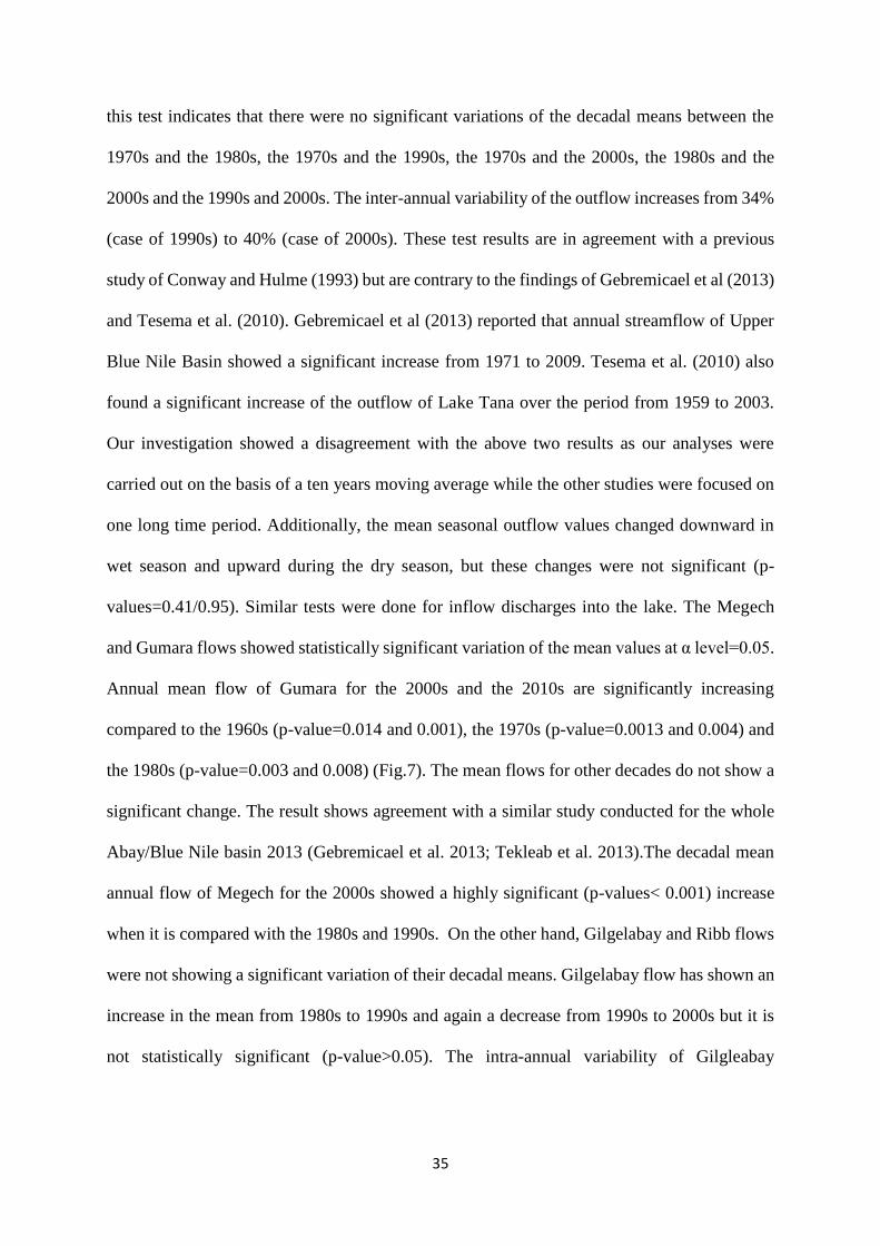
35
this test indicates that there were no significant variations of the decadal means between the
1970s and the 1980s, the 1970s and the 1990s, the 1970s and the 2000s, the 1980s and the
2000s and the 1990s and 2000s. The inter-annual variability of the outflow increases from 34%
(case of 1990s) to 40% (case of 2000s). These test results are in agreement with a previous
study of Conway and Hulme (1993) but are contrary to the findings of Gebremicael et al (2013)
and Tesema et al. (2010). Gebremicael et al (2013) reported that annual streamflow of Upper
Blue Nile Basin showed a significant increase from 1971 to 2009. Tesema et al. (2010) also
found a significant increase of the outflow of Lake Tana over the period from 1959 to 2003.
Our investigation showed a disagreement with the above two results as our analyses were
carried out on the basis of a ten years moving average while the other studies were focused on
one long time period. Additionally, the mean seasonal outflow values changed downward in
wet season and upward during the dry season, but these changes were not significant (p-
values=0.41/0.95). Similar tests were done for inflow discharges into the lake. The Megech
and Gumara flows showed statistically significant variation of the mean values at α level=0.05.
Annual mean flow of Gumara for the 2000s and the 2010s are significantly increasing
compared to the 1960s (p-value=0.014 and 0.001), the 1970s (p-value=0.0013 and 0.004) and
the 1980s (p-value=0.003 and 0.008) (Fig.7). The mean flows for other decades do not show a
significant change. The result shows agreement with a similar study conducted for the whole
Abay/Blue Nile basin 2013 (Gebremicael et al. 2013; Tekleab et al. 2013).The decadal mean
annual flow of Megech for the 2000s showed a highly significant (p-values< 0.001) increase
when it is compared with the 1980s and 1990s. On the other hand, Gilgelabay and Ribb flows
were not showing a significant variation of their decadal means. Gilgelabay flow has shown an
increase in the mean from 1980s to 1990s and again a decrease from 1990s to 2000s but it is
not statistically significant (p-value>0.05). The intra-annual variability of Gilgleabay
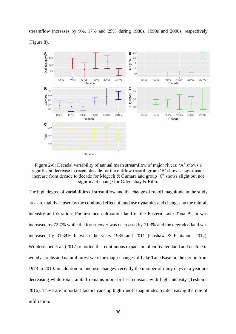
36
streamflow increases by 9%, 17% and 25% during 1980s, 1990s and 2000s, respectively
(Figure 8).
Figure 2-8: Decadal variability of annual mean streamflow of major rivers: ‘A’ shows a
significant decrease in recent decade for the outflow record, group ‘B’ shows a significant
increase from decade to decade for Megech & Gumara and group ‘C’ shows slight but not
significant change for Gilgelabay & Ribb.
The high degree of variabilities of streamflow and the change of runoff magnitude in the study
area are mainly caused by the combined effect of land use dynamics and changes on the rainfall
intensity and duration. For instance cultivation land of the Eastern Lake Tana Basin was
increased by 72.7% while the forest cover was decreased by 71.3% and the degraded land was
increased by 31.34% between the years 1985 and 2011 (Gashaw & Fentahun, 2014).
Woldesenbet et al. (2017) reported that continuous expansion of cultivated land and decline in
woody shrubs and natural forest were the major changes of Lake Tana Basin in the period from
1973 to 2010. In addition to land use changes, recently the number of rainy days in a year are
decreasing while total rainfall remains more or less constant with high intensity (Teshome
2016). These are important factors causing high runoff magnitudes by decreasing the rate of
infiltration.
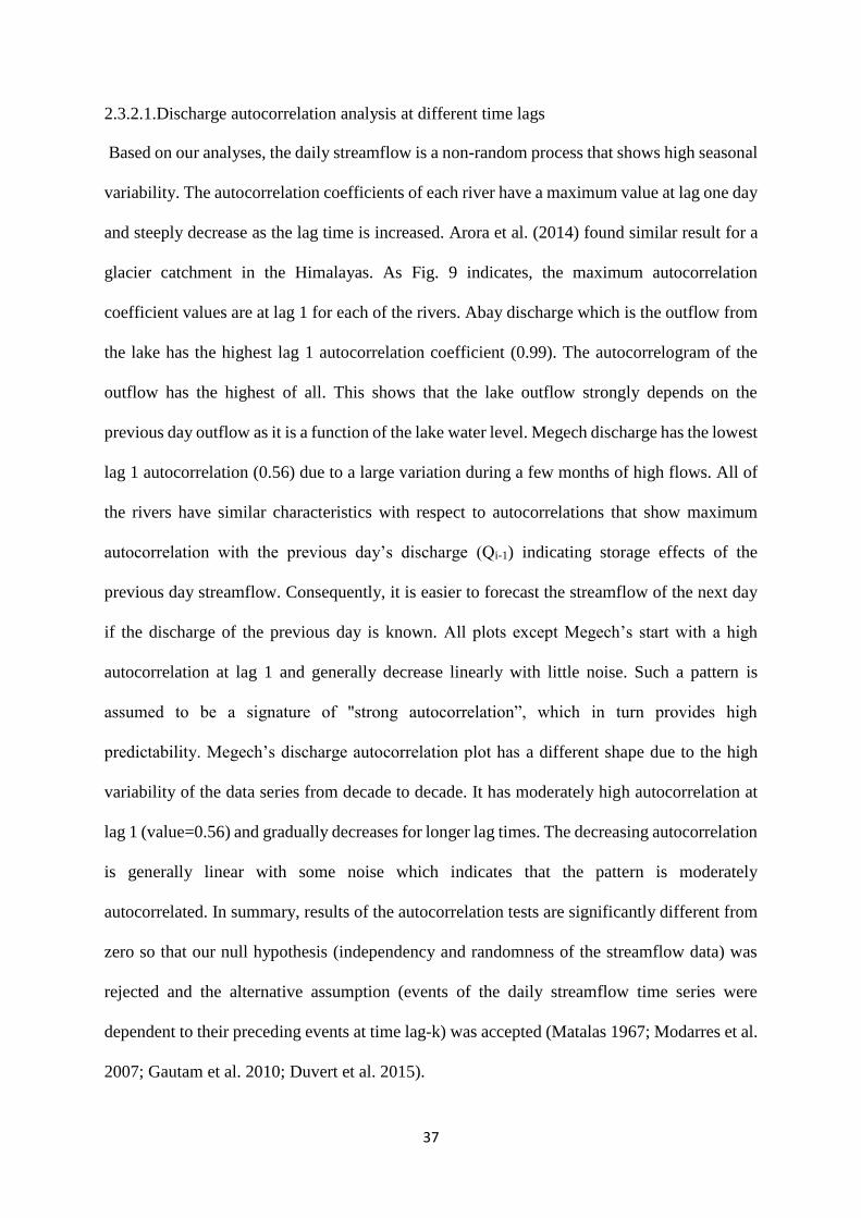
37
2.3.2.1.Discharge autocorrelation analysis at different time lags
Based on our analyses, the daily streamflow is a non-random process that shows high seasonal
variability. The autocorrelation coefficients of each river have a maximum value at lag one day
and steeply decrease as the lag time is increased. Arora et al. (2014) found similar result for a
glacier catchment in the Himalayas. As Fig. 9 indicates, the maximum autocorrelation
coefficient values are at lag 1 for each of the rivers. Abay discharge which is the outflow from
the lake has the highest lag 1 autocorrelation coefficient (0.99). The autocorrelogram of the
outflow has the highest of all. This shows that the lake outflow strongly depends on the
previous day outflow as it is a function of the lake water level. Megech discharge has the lowest
lag 1 autocorrelation (0.56) due to a large variation during a few months of high flows. All of
the rivers have similar characteristics with respect to autocorrelations that show maximum
autocorrelation with the previous day’s discharge (Qi-1) indicating storage effects of the
previous day streamflow. Consequently, it is easier to forecast the streamflow of the next day
if the discharge of the previous day is known. All plots except Megech’s start with a high
autocorrelation at lag 1 and generally decrease linearly with little noise. Such a pattern is
assumed to be a signature of "strong autocorrelation”, which in turn provides high
predictability. Megech’s discharge autocorrelation plot has a different shape due to the high
variability of the data series from decade to decade. It has moderately high autocorrelation at
lag 1 (value=0.56) and gradually decreases for longer lag times. The decreasing autocorrelation
is generally linear with some noise which indicates that the pattern is moderately
autocorrelated. In summary, results of the autocorrelation tests are significantly different from
zero so that our null hypothesis (independency and randomness of the streamflow data) was
rejected and the alternative assumption (events of the daily streamflow time series were
dependent to their preceding events at time lag-k) was accepted (Matalas 1967; Modarres et al.
2007; Gautam et al. 2010; Duvert et al. 2015).
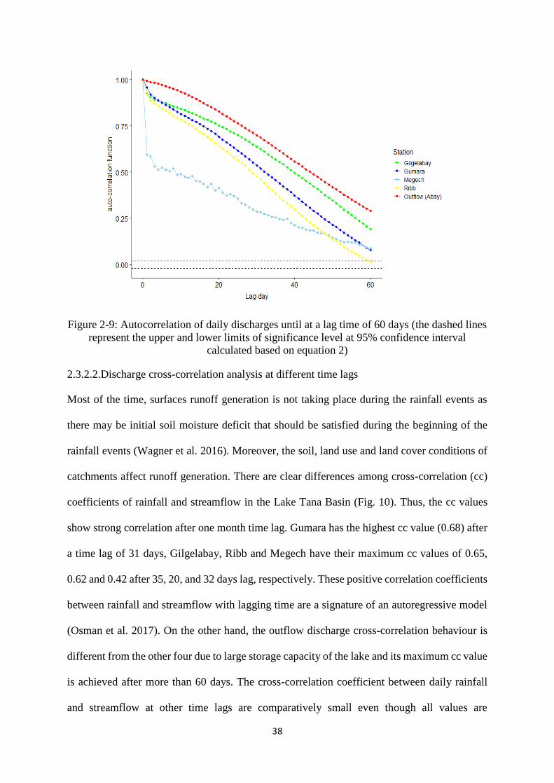
38
Figure 2-9: Autocorrelation of daily discharges until at a lag time of 60 days (the dashed lines
represent the upper and lower limits of significance level at 95% confidence interval
calculated based on equation 2)
2.3.2.2.Discharge cross-correlation analysis at different time lags
Most of the time, surfaces runoff generation is not taking place during the rainfall events as
there may be initial soil moisture deficit that should be satisfied during the beginning of the
rainfall events (Wagner et al. 2016). Moreover, the soil, land use and land cover conditions of
catchments affect runoff generation. There are clear differences among cross-correlation (cc)
coefficients of rainfall and streamflow in the Lake Tana Basin (Fig. 10). Thus, the cc values
show strong correlation after one month time lag. Gumara has the highest cc value (0.68) after
a time lag of 31 days, Gilgelabay, Ribb and Megech have their maximum cc values of 0.65,
0.62 and 0.42 after 35, 20, and 32 days lag, respectively. These positive correlation coefficients
between rainfall and streamflow with lagging time are a signature of an autoregressive model
(Osman et al. 2017). On the other hand, the outflow discharge cross-correlation behaviour is
different from the other four due to large storage capacity of the lake and its maximum cc value
is achieved after more than 60 days. The cross-correlation coefficient between daily rainfall
and streamflow at other time lags are comparatively small even though all values are
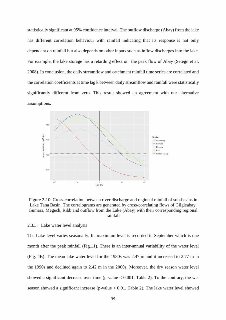
39
statistically significant at 95% confidence interval. The outflow discharge (Abay) from the lake
has different correlation behaviour with rainfall indicating that its response is not only
dependent on rainfall but also depends on other inputs such as inflow discharges into the lake.
For example, the lake storage has a retarding effect on the peak flow of Abay (Setegn et al.
2008). In conclusion, the daily streamflow and catchment rainfall time series are correlated and
the correlation coefficients at time lag k between daily streamflow and rainfall were statistically
significantly different from zero. This result showed an agreement with our alternative
assumptions.
Figure 2-10: Cross-correlation between river discharge and regional rainfall of sub-basins in
Lake Tana Basin. The correlograms are generated by cross-correlating flows of Gilgleabay,
Gumara, Megech, Ribb and outflow from the Lake (Abay) with their corresponding regional
rainfall
2.3.3. Lake water level analysis
The Lake level varies seasonally. Its maximum level is recorded in September which is one
month after the peak rainfall (Fig.11). There is an inter-annual variability of the water level
(Fig. 4B). The mean lake water level for the 1980s was 2.47 m and it increased to 2.77 m in
the 1990s and declined again to 2.42 m in the 2000s. Moreover, the dry season water level
showed a significant decrease over time (p-value < 0.001, Table 2). To the contrary, the wet
season showed a significant increase (p-value < 0.01, Table 2). The lake water level showed
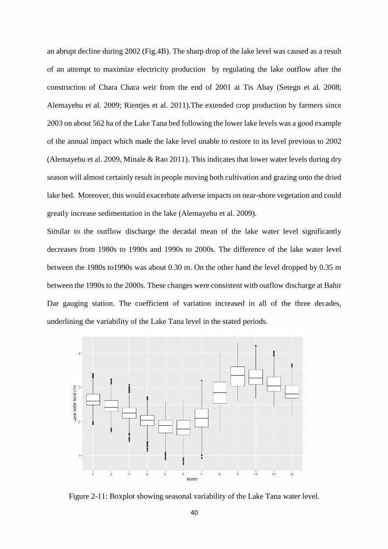
40
an abrupt decline during 2002 (Fig.4B). The sharp drop of the lake level was caused as a result
of an attempt to maximize electricity production by regulating the lake outflow after the
construction of Chara Chara weir from the end of 2001 at Tis Abay (Setegn et al. 2008;
Alemayehu et al. 2009; Rientjes et al. 2011).The extended crop production by farmers since
2003 on about 562 ha of the Lake Tana bed following the lower lake levels was a good example
of the annual impact which made the lake level unable to restore to its level previous to 2002
(Alemayehu et al. 2009, Minale & Rao 2011). This indicates that lower water levels during dry
season will almost certainly result in people moving both cultivation and grazing onto the dried
lake bed. Moreover, this would exacerbate adverse impacts on near-shore vegetation and could
greatly increase sedimentation in the lake (Alemayehu et al. 2009).
Similar to the outflow discharge the decadal mean of the lake water level significantly
decreases from 1980s to 1990s and 1990s to 2000s. The difference of the lake water level
between the 1980s to1990s was about 0.30 m. On the other hand the level dropped by 0.35 m
between the 1990s to the 2000s. These changes were consistent with outflow discharge at Bahir
Dar gauging station. The coefficient of variation increased in all of the three decades,
underlining the variability of the Lake Tana level in the stated periods.
Figure 2-11: Boxplot showing seasonal variability of the Lake Tana water level.
41
2.4. Conclusions
In this study, rainfall, lake level and streamflow data of several years were analysed. The
rainfall pattern in the basin is monomodal with a peak in July or August. The direction of Mann-
Kendall trend test vary among annual, dry and wet seasons as well as daily rainfall and
streamflows implying that the time period of investigation matters. The annual rainfall change
over time is mostly not statistically significant. About 55% of the rainfall stations showed a
positive trend and only three of them (Enjibara & Zege at α = 0.05, Gondar α = 0.01) showed
significant changes. The remaining 45% of the station showed insignificant downward trends
except Addis Zemen. But the seasonal changes were significant for eight stations (Table 1).
The summer rainfall changes could be related to SST variation. The maximum lake water level
is recorded in the month of September, following the maximum amount of rainfall in the
previous months. The annual mean lake water level has shown a decreasing trend from decade
to decade and since the year 2002. The long-term annual mean lake water level is about 2.6 m.
The autocorrelation coefficient values of daily rainfall and streamflow are decreasing linearly
as the time lag increases but they are significantly different from zero indicating that the data
come from an underlying autoregressive process with moderate to strong positive
autocorrelation (Matalas 1967; Modarres 2007; Gautam et al. 2010) . The streamflow values
have their maximum cross-correlation coefficient after 20- 60 days due to basin lag time caused
by the shape of the catchment, size of the drainage basin, soil and vegetation cover.
In general the Lake Tana Basin is a hydrologically highly dynamic area that shows high
variability on the daily, monthly and yearly streamflow and the lake water level. The changes
in streamflow and the lake water level are mainly linked to intensive land use changes such as
expansion of intensive agriculture, urbanization and deforestation as well as change in the
number of rainfall days and intensity. Improvements in agricultural water management could
help to increase the water use efficiency, which consequently may contribute to mitigate the

42
decreasing trends.
43
3. Modeling the impact of agricultural crops on the spatial and seasonal
variability of water balance components in the Lake Tana Basin,
Ethiopia
*Tibebe B. Tigabu, Paul D. Wagner, Georg Hörmann and Nicola Fohrer
Department of Hydrology and Water Resources Management, Institute for Natural Resource
Conservation, Kiel University, D-24118 Kiel, Germany
Address to correspondence author: Tibebe Tigabu, Department of Hydrology and Water
Resources Management, Institute of Natural Resource Conservation, CAU, D-24118 Kiel,
Germany, E-mail: [email protected]
Hydrology Research (2019) 50 (5): 1376–1396
Submitted: December 18 2018 - Accepted: July 29 2019- printed October 2019, 50(5),
pp.1376-1396.
44
Abstract
The Lake Tana basin hosts more than 3 million people and it is well known for its water
resource potential by the Ethiopian government. The major economic activity in the region is
agriculture, but the effect of agricultural crops on water resources is poorly understood.
Understanding the crop water interaction is important to design proper water management
plans. Therefore, the primary objective of this research is to investigate the effect of different
agricultural crops on the spatial and seasonal variability of water balance components of
Gilgelabay, Gumara, and Ribb catchment areas of Lake Tana Basin, Ethiopia. To this end, the
hydrologic model SWAT was used to simulate the water fluxes between 1980 and 2014. The
water balance components, which were mapped for each hydrologic response unit, indicated
the spatial variations of water fluxes in the study. Cereal crops like teff and millet had
significant effect in enhancing groundwater recharge, whereas leguminous crops like peas had
significant impact in increasing runoff generation. Moreover, the model outputs showed that
the total streamflow is dominated by baseflow and about 13%, 9%, and 7% of the annual
rainfall goes to the deep aquifer system of Gilgelabay, Gumara, and Ribb catchment areas,
respectively.
Keywords: groundwater recharge; land use land cover; SWAT; Lake Tana
45
3.1. Introduction
Agriculture, food production and water are inseparably linked (Watts et al. 2015). Water use
in agriculture accounts for 70% of the global total water use (Hatfield 2014). Consequently, it
has a significant impact on the water balance components. Agricultural land use affects the
hydrologic cycle in terms of the partitioning of rainfall between evapotranspiration, runoff, and
groundwater recharge (Watts et al. 2015). The quality of surface water and groundwater has
generally declined in recent decades mainly due to an increase of agricultural and industrial
activities (Parris 2011). The complete drying up of Haramaya Lake in Eastern Ethiopia since
2005 is an example for the consequences of decreasing groundwater levels due to over-
pumping for agriculture and household use (Abebe et al. 2014). To prepare for the future and
avoid past mistakes, modeling the effect of agricultural crops on the spatial and seasonal
variation of water balance components is required. Although several water balance studies have
been performed globally, only a few of them focused on the effect of agricultural crops on
water balance components. For example, Zhao et al. (2010), studied the effect of vegetation
change and climate variability on streamflow of seven paired catchments in Australia, New
Zealand, and South Africa. Li et al. 2019 also studied the spatio-temporal impacts of land use
and land cover changes on the hydrology of the Wei River Basin, China.
The agriculture sector plays a central role in the Ethiopian economy, where about 85% of all
employment relies on it (FAO, 2014). This economic sector is dominated by small-scale
farmers who depend on rain-fed mixed farming. Crop production accounts for about 60% of
the agricultural outputs (Gebre-Selasie and Bekele 2012). The crop productivity varies with the
availability of water and water use in agriculture. Although Ethiopia is perceived as the water
tower of Eastern Africa, temporal variability (seasonality) and uneven spatial distribution of
water resources remain the primary challenge. Availability of water is highly dependent on the
seasonality and inter-annual variability of rainfall and streamflow. The temporal variabilities
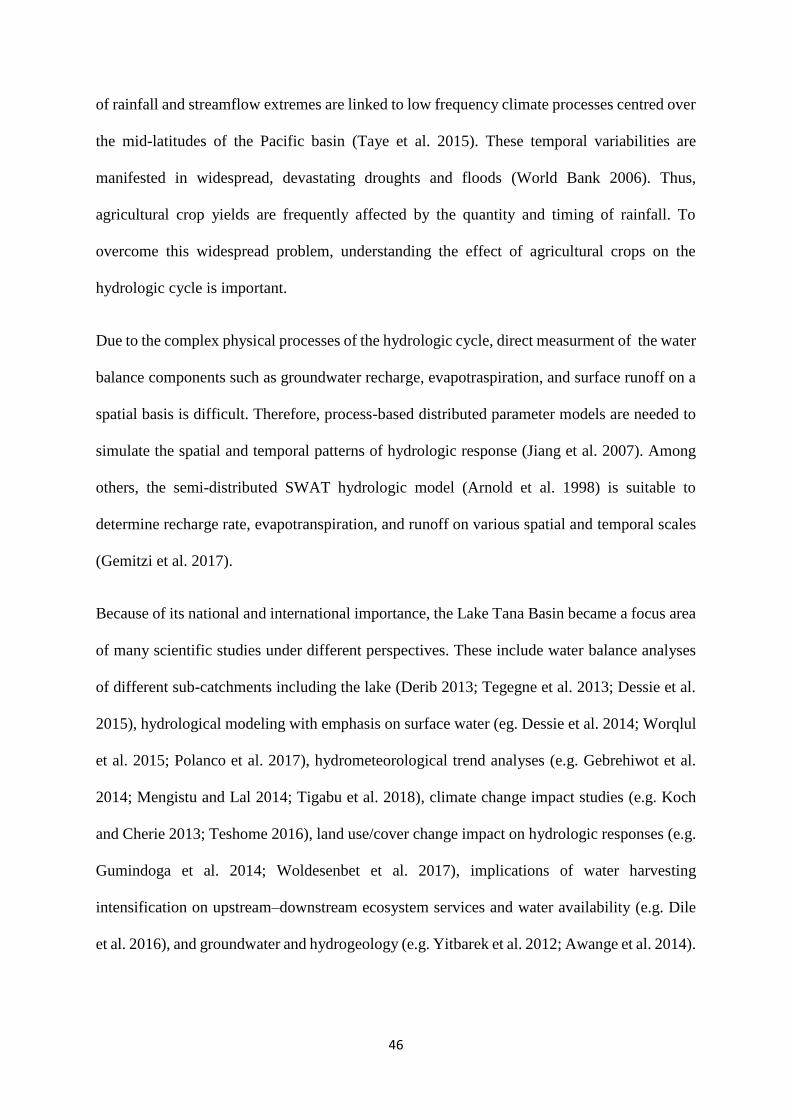
46
of rainfall and streamflow extremes are linked to low frequency climate processes centred over
the mid-latitudes of the Pacific basin (Taye et al. 2015). These temporal variabilities are
manifested in widespread, devastating droughts and floods (World Bank 2006). Thus,
agricultural crop yields are frequently affected by the quantity and timing of rainfall. To
overcome this widespread problem, understanding the effect of agricultural crops on the
hydrologic cycle is important.
Due to the complex physical processes of the hydrologic cycle, direct measurment of the water
balance components such as groundwater recharge, evapotraspiration, and surface runoff on a
spatial basis is difficult. Therefore, process-based distributed parameter models are needed to
simulate the spatial and temporal patterns of hydrologic response (Jiang et al. 2007). Among
others, the semi-distributed SWAT hydrologic model (Arnold et al. 1998) is suitable to
determine recharge rate, evapotranspiration, and runoff on various spatial and temporal scales
(Gemitzi et al. 2017).
Because of its national and international importance, the Lake Tana Basin became a focus area
of many scientific studies under different perspectives. These include water balance analyses
of different sub-catchments including the lake (Derib 2013; Tegegne et al. 2013; Dessie et al.
2015), hydrological modeling with emphasis on surface water (eg. Dessie et al. 2014; Worqlul
et al. 2015; Polanco et al. 2017), hydrometeorological trend analyses (e.g. Gebrehiwot et al.
2014; Mengistu and Lal 2014; Tigabu et al. 2018), climate change impact studies (e.g. Koch
and Cherie 2013; Teshome 2016), land use/cover change impact on hydrologic responses (e.g.
Gumindoga et al. 2014; Woldesenbet et al. 2017), implications of water harvesting
intensification on upstream–downstream ecosystem services and water availability (e.g. Dile
et al. 2016), and groundwater and hydrogeology (e.g. Yitbarek et al. 2012; Awange et al. 2014).
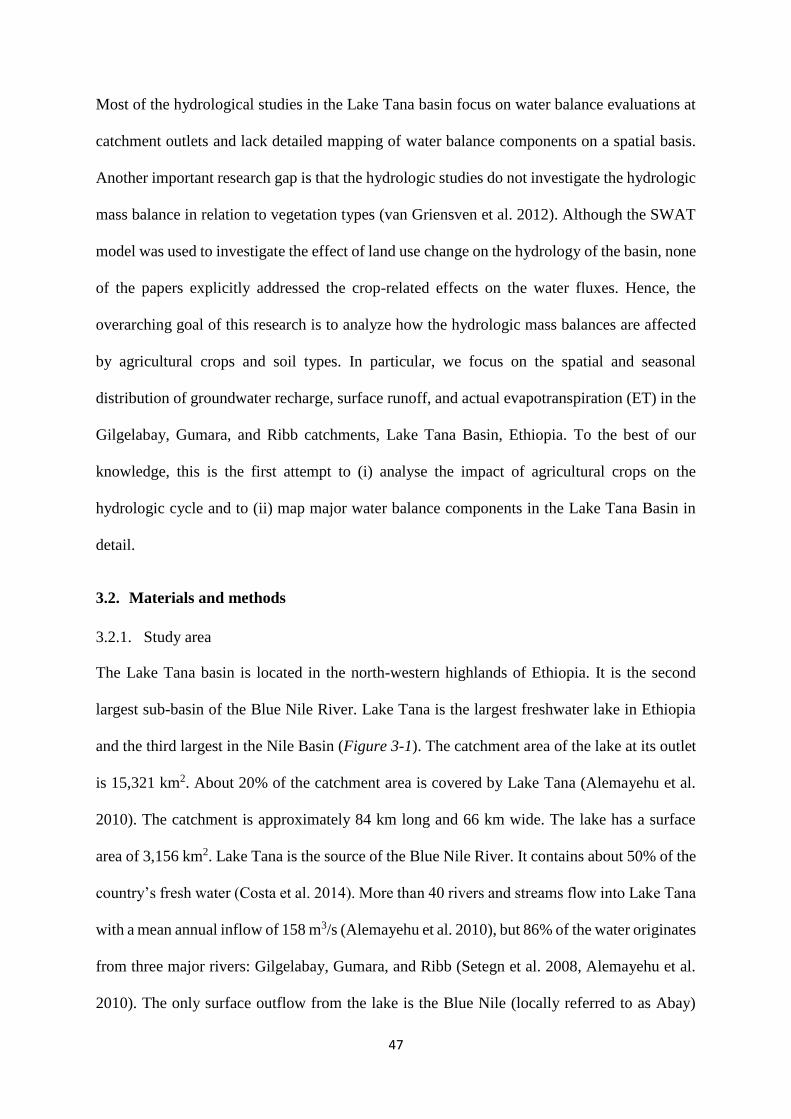
47
Most of the hydrological studies in the Lake Tana basin focus on water balance evaluations at
catchment outlets and lack detailed mapping of water balance components on a spatial basis.
Another important research gap is that the hydrologic studies do not investigate the hydrologic
mass balance in relation to vegetation types (van Griensven et al. 2012). Although the SWAT
model was used to investigate the effect of land use change on the hydrology of the basin, none
of the papers explicitly addressed the crop-related effects on the water fluxes. Hence, the
overarching goal of this research is to analyze how the hydrologic mass balances are affected
by agricultural crops and soil types. In particular, we focus on the spatial and seasonal
distribution of groundwater recharge, surface runoff, and actual evapotranspiration (ET) in the
Gilgelabay, Gumara, and Ribb catchments, Lake Tana Basin, Ethiopia. To the best of our
knowledge, this is the first attempt to (i) analyse the impact of agricultural crops on the
hydrologic cycle and to (ii) map major water balance components in the Lake Tana Basin in
detail.
3.2. Materials and methods
3.2.1. Study area
The Lake Tana basin is located in the north-western highlands of Ethiopia. It is the second
largest sub-basin of the Blue Nile River. Lake Tana is the largest freshwater lake in Ethiopia
and the third largest in the Nile Basin (Figure 3-1). The catchment area of the lake at its outlet
is 15,321 km2. About 20% of the catchment area is covered by Lake Tana (Alemayehu et al.
2010). The catchment is approximately 84 km long and 66 km wide. The lake has a surface
area of 3,156 km2. Lake Tana is the source of the Blue Nile River. It contains about 50% of the
country’s fresh water (Costa et al. 2014). More than 40 rivers and streams flow into Lake Tana
with a mean annual inflow of 158 m3/s (Alemayehu et al. 2010), but 86% of the water originates
from three major rivers: Gilgelabay, Gumara, and Ribb (Setegn et al. 2008, Alemayehu et al.
2010). The only surface outflow from the lake is the Blue Nile (locally referred to as Abay)
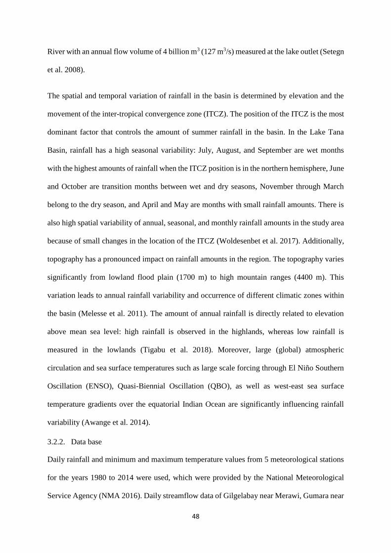
48
River with an annual flow volume of 4 billion m3 (127 m3/s) measured at the lake outlet (Setegn
et al. 2008).
The spatial and temporal variation of rainfall in the basin is determined by elevation and the
movement of the inter-tropical convergence zone (ITCZ). The position of the ITCZ is the most
dominant factor that controls the amount of summer rainfall in the basin. In the Lake Tana
Basin, rainfall has a high seasonal variability: July, August, and September are wet months
with the highest amounts of rainfall when the ITCZ position is in the northern hemisphere, June
and October are transition months between wet and dry seasons, November through March
belong to the dry season, and April and May are months with small rainfall amounts. There is
also high spatial variability of annual, seasonal, and monthly rainfall amounts in the study area
because of small changes in the location of the ITCZ (Woldesenbet et al. 2017). Additionally,
topography has a pronounced impact on rainfall amounts in the region. The topography varies
significantly from lowland flood plain (1700 m) to high mountain ranges (4400 m). This
variation leads to annual rainfall variability and occurrence of different climatic zones within
the basin (Melesse et al. 2011). The amount of annual rainfall is directly related to elevation
above mean sea level: high rainfall is observed in the highlands, whereas low rainfall is
measured in the lowlands (Tigabu et al. 2018). Moreover, large (global) atmospheric
circulation and sea surface temperatures such as large scale forcing through El Niño Southern
Oscillation (ENSO), Quasi-Biennial Oscillation (QBO), as well as west-east sea surface
temperature gradients over the equatorial Indian Ocean are significantly influencing rainfall
variability (Awange et al. 2014).
3.2.2. Data base
Daily rainfall and minimum and maximum temperature values from 5 meteorological stations
for the years 1980 to 2014 were used, which were provided by the National Meteorological
Service Agency (NMA 2016). Daily streamflow data of Gilgelabay near Merawi, Gumara near
49
Bahirdar, and Ribb near Addis Zemen gauging stations for the years 1980 to 2014 were
obtained from the Department of Hydrology, Ministry of Water, Irrigation and Electricity of
the Ethiopian Government (MoWIE 2016).
Figure 3-1: Location map and major tributaries of Lake Tana including river gauging and
weather stations
Land use and land cover as well as soil data at a scale of 1:50000 were provided by the Amhara
Design & Supervision Works Enterprise (ADSWE 2017). About 60.2% of the basin is covered
by agricultural land. This area is further classified as intensively cultivated (37.3%), moderately
cultivated (16.0%), and farm villages (6.9%) (Figure 3-2). The soils in the study area are highly
heterogeneous. Eutric Leptosols are covering around 50% of the total area followed by Eutric
Nitosols (13%). The soil textural classes vary from sandy-loam to clay (Eutric Regosols
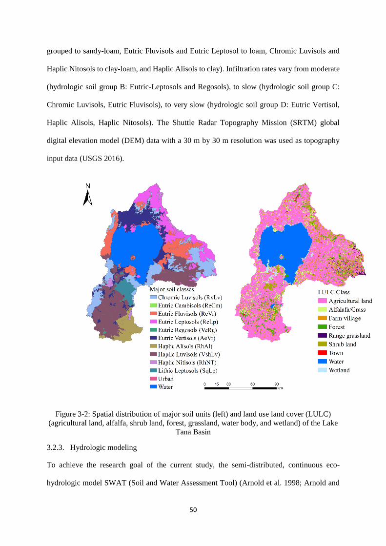
50
grouped to sandy-loam, Eutric Fluvisols and Eutric Leptosol to loam, Chromic Luvisols and
Haplic Nitosols to clay-loam, and Haplic Alisols to clay). Infiltration rates vary from moderate
(hydrologic soil group B: Eutric-Leptosols and Regosols), to slow (hydrologic soil group C:
Chromic Luvisols, Eutric Fluvisols), to very slow (hydrologic soil group D: Eutric Vertisol,
Haplic Alisols, Haplic Nitosols). The Shuttle Radar Topography Mission (SRTM) global
digital elevation model (DEM) data with a 30 m by 30 m resolution was used as topography
input data (USGS 2016).
Figure 3-2: Spatial distribution of major soil units (left) and land use land cover (LULC)
(agricultural land, alfalfa, shrub land, forest, grassland, water body, and wetland) of the Lake
Tana Basin
3.2.3. Hydrologic modeling
To achieve the research goal of the current study, the semi-distributed, continuous eco-
hydrologic model SWAT (Soil and Water Assessment Tool) (Arnold et al. 1998; Arnold and
51
Fohrer 2005) was used. The model is capable of simulating spatially distributed water balance
components based on hydrological response units (HRUs). Four main steps comprise the
modeling approach:
1) Hydrological model setup: Three independent SWAT models were setup for the three
catchments Gilgelabay, Gumara, and Ribb based on available climate, land use, soil, and digital
elevation model data. No water withdrawal was considered in the model setup as this
information was not available. The three independent model setups were used to better
represent each catchment, e.g. by a more precise representation of the stream network. In this
study, the SWAT model was not setup for the entire Lake Tana basin. Although there is
measured streamflow data at the lake outlet, it could not be used to calibrate and validate the
SWAT model as there is water abstraction from Lake Tana for different purposes and there is
no information about the amount of water withdrawn for such purposes (Setegn et al. 2008).
ArcSWAT 12.102.19 was used to compile the SWAT input files and SWAT2012 revision 664
was used to run the simulations. Each catchment was divided into sub-basins. Nine LULC units
were used as input for the hydrologic models (Figure 3-2). Agricultural land is the dominant
land use class in the study area (ADSWE 2017). We further split the agricultural land use class
into different crop units based on their aggregate areal coverage proportions. Splitting of the
agricultural land at this step allows for a detailed consideration of the spatial distribution of the
crop units in each HRU (Guse et al. 2015). Cereal crops, vegetables, root crops, and fruit crops
are the common agricultural products in Ethiopia. Cereal crops including teff, corn, sorghum,
and wheat are the dominant cereal crops both with regard to yields and area coverage. About
24%, 17%, 15%, and 13% of the national agricultural land are covered by teff, corn, sorghum,
and wheat, respectively (CSA 2017). To account for the spatial variation of these crops, we
calculated their coverage for each catchment based on the respective Administrative Zone of
the Amhara Regional State Government (Awi, West Gojam, and South Gondar). The crop
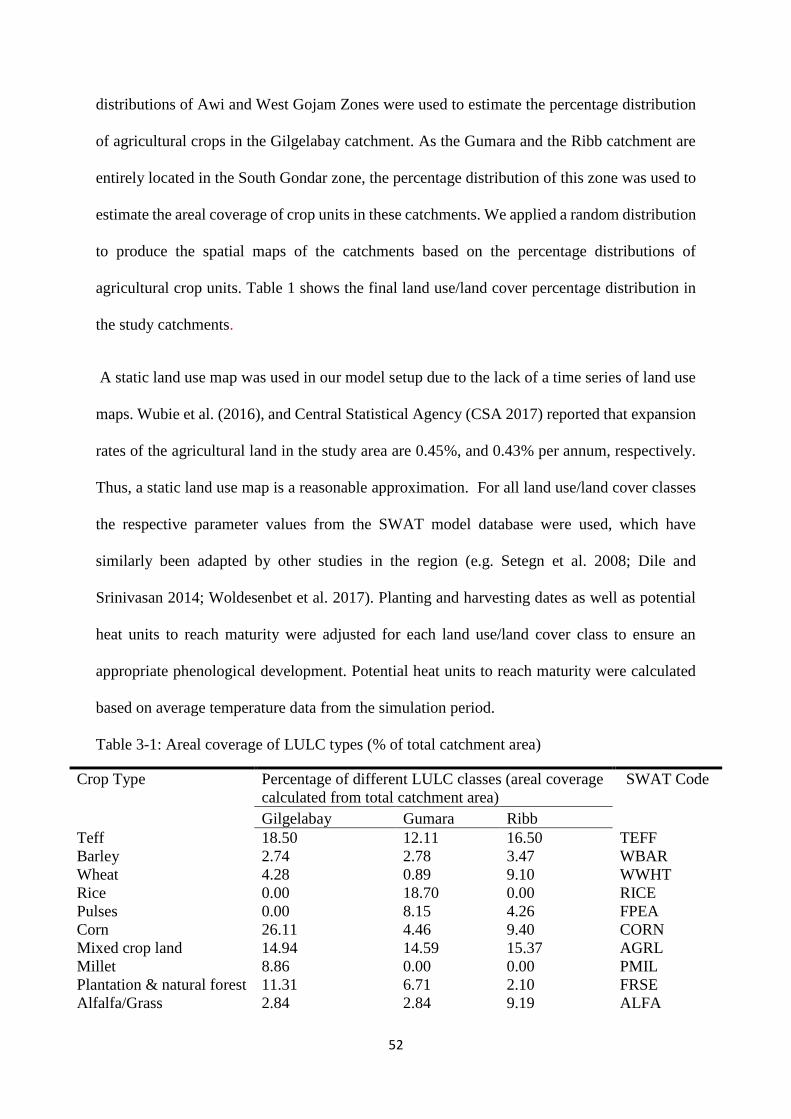
52
distributions of Awi and West Gojam Zones were used to estimate the percentage distribution
of agricultural crops in the Gilgelabay catchment. As the Gumara and the Ribb catchment are
entirely located in the South Gondar zone, the percentage distribution of this zone was used to
estimate the areal coverage of crop units in these catchments. We applied a random distribution
to produce the spatial maps of the catchments based on the percentage distributions of
agricultural crop units. Table 1 shows the final land use/land cover percentage distribution in
the study catchments.
A static land use map was used in our model setup due to the lack of a time series of land use
maps. Wubie et al. (2016), and Central Statistical Agency (CSA 2017) reported that expansion
rates of the agricultural land in the study area are 0.45%, and 0.43% per annum, respectively.
Thus, a static land use map is a reasonable approximation. For all land use/land cover classes
the respective parameter values from the SWAT model database were used, which have
similarly been adapted by other studies in the region (e.g. Setegn et al. 2008; Dile and
Srinivasan 2014; Woldesenbet et al. 2017). Planting and harvesting dates as well as potential
heat units to reach maturity were adjusted for each land use/land cover class to ensure an
appropriate phenological development. Potential heat units to reach maturity were calculated
based on average temperature data from the simulation period.
Table 3-1: Areal coverage of LULC types (% of total catchment area)
Crop Type Percentage of different LULC classes (areal coverage
calculated from total catchment area)
SWAT Code
Gilgelabay Gumara Ribb
Teff 18.50 12.11 16.50 TEFF
Barley 2.74 2.78 3.47 WBAR
Wheat 4.28 0.89 9.10 WWHT
Rice 0.00 18.70 0.00 RICE
Pulses 0.00 8.15 4.26 FPEA
Corn 26.11 4.46 9.40 CORN
Mixed crop land 14.94 14.59 15.37 AGRL
Millet 8.86 0.00 0.00 PMIL
Plantation & natural forest 11.31 6.71 2.10 FRSE
Alfalfa/Grass 2.84 2.84 9.19 ALFA
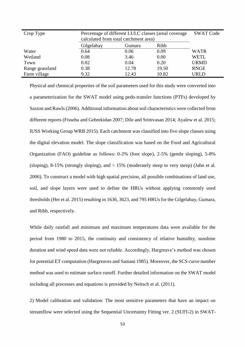
53
Crop Type Percentage of different LULC classes (areal coverage
calculated from total catchment area)
SWAT Code
Gilgelabay Gumara Ribb
Water 0.64 0.06 0.09 WATR
Wetland 0.08 3.46 0.00 WETL
Town 0.02 0.04 0.20 URMD
Range grassland 0.38 12.78 19.50 RNGE
Farm village 9.32 12.43 10.82 URLD
Physical and chemical properties of the soil parameters used for this study were converted into
a parameterization for the SWAT model using pedo-transfer functions (PTFs) developed by
Saxton and Rawls (2006). Additional information about soil characteristics were collected from
different reports (Fisseha and Gebrekidan 2007; Dile and Srinivasan 2014; Ayalew et al. 2015;
IUSS Working Group WRB 2015). Each catchment was classified into five slope classes using
the digital elevation model. The slope classification was based on the Food and Agricultural
Organization (FAO) guideline as follows: 0-2% (foot slope), 2-5% (gentle sloping), 5-8%
(sloping), 8-15% (strongly sloping), and > 15% (moderately steep to very steep) (Jahn et al.
2006). To construct a model with high spatial precision, all possible combinations of land use,
soil, and slope layers were used to define the HRUs without applying commonly used
thresholds (Her et al. 2015) resulting in 1636, 3623, and 795 HRUs for the Gilgelabay, Gumara,
and Ribb, respectively.
While daily rainfall and minimum and maximum temperatures data were available for the
period from 1980 to 2015, the continuity and consistency of relative humidity, sunshine
duration and wind speed data were not reliable. Accordingly, Hargreave’s method was chosen
for potential ET computation (Hargreaves and Samani 1985). Moreover, the SCS curve number
method was used to estimate surface runoff. Further detailed information on the SWAT model
including all processes and equations is provided by Neitsch et al. (2011).
2) Model calibration and validation: The most sensitive parameters that have an impact on
streamflow were selected using the Sequential Uncertainty Fitting ver. 2 (SUFI-2) in SWAT-
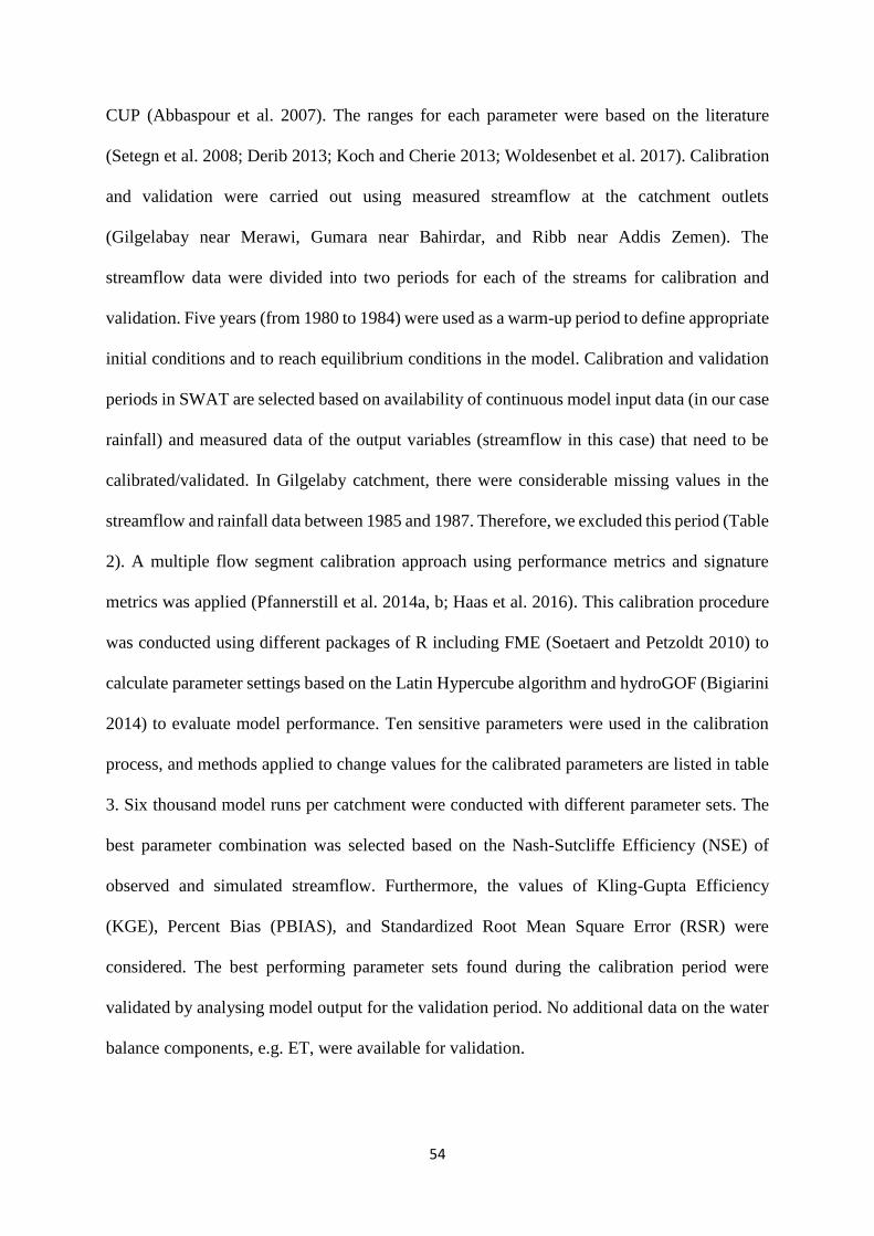
54
CUP (Abbaspour et al. 2007). The ranges for each parameter were based on the literature
(Setegn et al. 2008; Derib 2013; Koch and Cherie 2013; Woldesenbet et al. 2017). Calibration
and validation were carried out using measured streamflow at the catchment outlets
(Gilgelabay near Merawi, Gumara near Bahirdar, and Ribb near Addis Zemen). The
streamflow data were divided into two periods for each of the streams for calibration and
validation. Five years (from 1980 to 1984) were used as a warm-up period to define appropriate
initial conditions and to reach equilibrium conditions in the model. Calibration and validation
periods in SWAT are selected based on availability of continuous model input data (in our case
rainfall) and measured data of the output variables (streamflow in this case) that need to be
calibrated/validated. In Gilgelaby catchment, there were considerable missing values in the
streamflow and rainfall data between 1985 and 1987. Therefore, we excluded this period (Table
2). A multiple flow segment calibration approach using performance metrics and signature
metrics was applied (Pfannerstill et al. 2014a, b; Haas et al. 2016). This calibration procedure
was conducted using different packages of R including FME (Soetaert and Petzoldt 2010) to
calculate parameter settings based on the Latin Hypercube algorithm and hydroGOF (Bigiarini
2014) to evaluate model performance. Ten sensitive parameters were used in the calibration
process, and methods applied to change values for the calibrated parameters are listed in table
3. Six thousand model runs per catchment were conducted with different parameter sets. The
best parameter combination was selected based on the Nash-Sutcliffe Efficiency (NSE) of
observed and simulated streamflow. Furthermore, the values of Kling-Gupta Efficiency
(KGE), Percent Bias (PBIAS), and Standardized Root Mean Square Error (RSR) were
considered. The best performing parameter sets found during the calibration period were
validated by analysing model output for the validation period. No additional data on the water
balance components, e.g. ET, were available for validation.
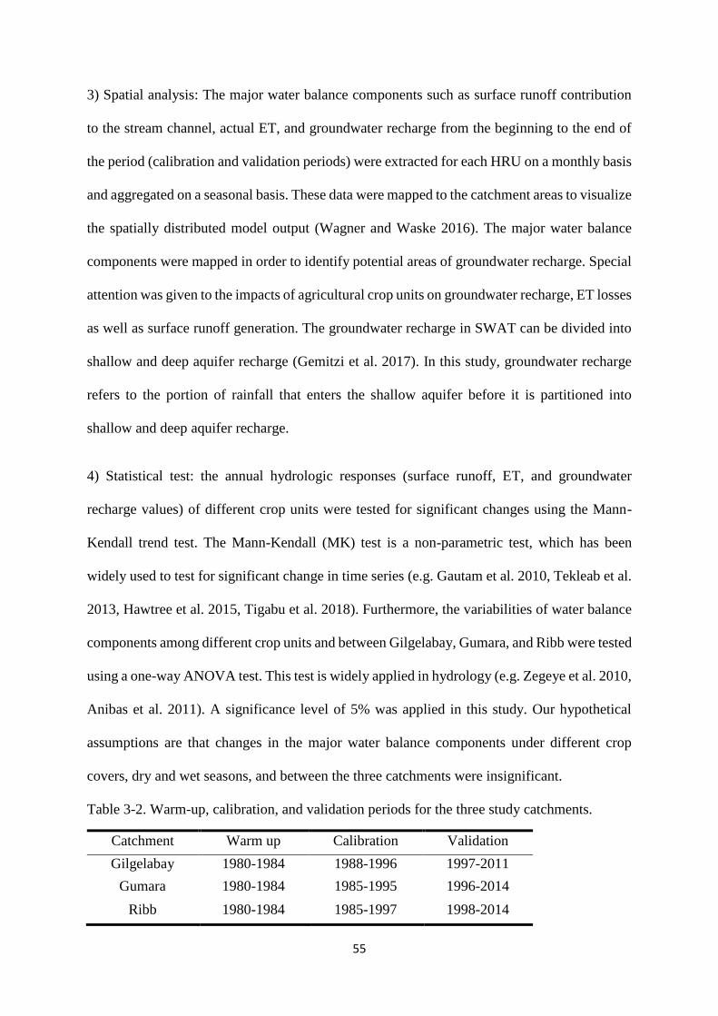
55
3) Spatial analysis: The major water balance components such as surface runoff contribution
to the stream channel, actual ET, and groundwater recharge from the beginning to the end of
the period (calibration and validation periods) were extracted for each HRU on a monthly basis
and aggregated on a seasonal basis. These data were mapped to the catchment areas to visualize
the spatially distributed model output (Wagner and Waske 2016). The major water balance
components were mapped in order to identify potential areas of groundwater recharge. Special
attention was given to the impacts of agricultural crop units on groundwater recharge, ET losses
as well as surface runoff generation. The groundwater recharge in SWAT can be divided into
shallow and deep aquifer recharge (Gemitzi et al. 2017). In this study, groundwater recharge
refers to the portion of rainfall that enters the shallow aquifer before it is partitioned into
shallow and deep aquifer recharge.
4) Statistical test: the annual hydrologic responses (surface runoff, ET, and groundwater
recharge values) of different crop units were tested for significant changes using the Mann-
Kendall trend test. The Mann-Kendall (MK) test is a non-parametric test, which has been
widely used to test for significant change in time series (e.g. Gautam et al. 2010, Tekleab et al.
2013, Hawtree et al. 2015, Tigabu et al. 2018). Furthermore, the variabilities of water balance
components among different crop units and between Gilgelabay, Gumara, and Ribb were tested
using a one-way ANOVA test. This test is widely applied in hydrology (e.g. Zegeye et al. 2010,
Anibas et al. 2011). A significance level of 5% was applied in this study. Our hypothetical
assumptions are that changes in the major water balance components under different crop
covers, dry and wet seasons, and between the three catchments were insignificant.
Table 3-2. Warm-up, calibration, and validation periods for the three study catchments.
Catchment Warm up Calibration Validation
Gilgelabay 1980-1984 1988-1996 1997-2011
Gumara 1980-1984 1985-1995 1996-2014
Ribb 1980-1984 1985-1997 1998-2014
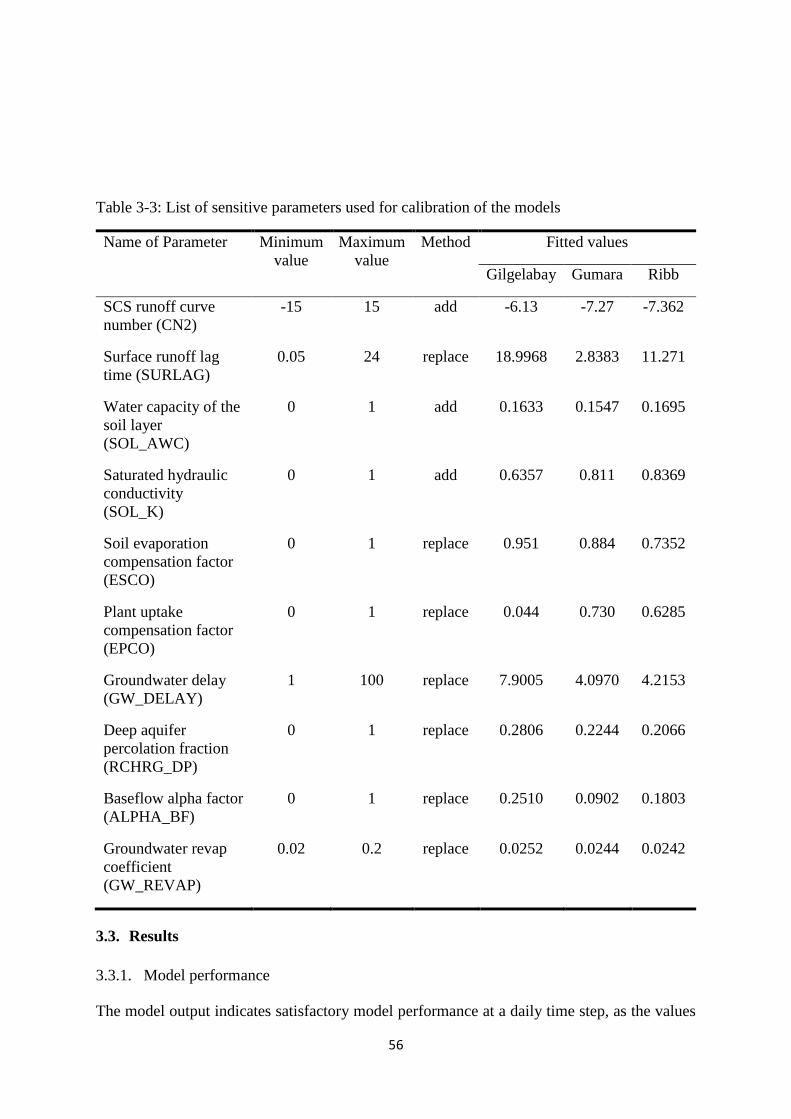
56
Table 3-3: List of sensitive parameters used for calibration of the models
Name of Parameter Minimum
value
Maximum
value
Method Fitted values
Gilgelabay Gumara Ribb
SCS runoff curve
number (CN2)
-15 15 add -6.13 -7.27 -7.362
Surface runoff lag
time (SURLAG)
0.05 24 replace 18.9968 2.8383 11.271
Water capacity of the
soil layer
(SOL_AWC)
0 1 add 0.1633 0.1547 0.1695
Saturated hydraulic
conductivity
(SOL_K)
0 1 add 0.6357 0.811 0.8369
Soil evaporation
compensation factor
(ESCO)
0 1 replace 0.951 0.884 0.7352
Plant uptake
compensation factor
(EPCO)
0 1 replace 0.044 0.730 0.6285
Groundwater delay
(GW_DELAY)
1 100 replace 7.9005 4.0970 4.2153
Deep aquifer
percolation fraction
(RCHRG_DP)
0 1 replace 0.2806 0.2244 0.2066
Baseflow alpha factor
(ALPHA_BF)
0 1 replace 0.2510 0.0902 0.1803
Groundwater revap
coefficient
(GW_REVAP)
0.02 0.2 replace 0.0252 0.0244 0.0242
3.3. Results
3.3.1. Model performance
The model output indicates satisfactory model performance at a daily time step, as the values
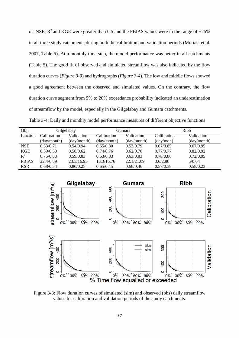
57
of NSE, R2 and KGE were greater than 0.5 and the PBIAS values were in the range of ±25%
in all three study catchments during both the calibration and validation periods (Moriasi et al.
2007, Table 5). At a monthly time step, the model performance was better in all catchments
(Table 5). The good fit of observed and simulated streamflow was also indicated by the flow
duration curves (Figure 3-3) and hydrographs (Figure 3-4). The low and middle flows showed
a good agreement between the observed and simulated values. On the contrary, the flow
duration curve segment from 5% to 20% exceedance probability indicated an underestimation
of streamflow by the model, especially in the Gilgelabay and Gumara catchments.
Table 3-4: Daily and monthly model performance measures of different objective functions
Obj.
function
Gilgelabay Gumara Ribb
Calibration
(day/month)
Validation
(day/month)
Calibration
(day/month)
Validation
(day/month)
Calibration
(day/mon)
Validation
(day/month)
NSE 0.53/0.71 0.54/0.94 0.65/0.80 0.53/0.79 0.67/0.85 0.67/0.95
KGE 0.59/0.50 0.58/0.62 0.74/0.76 0.62/0.70 0.77/0.77 0.82/0.92
R2 0.75/0.83 0.59/0.83 0.63/0.83 0.63/0.83 0.78/0.86 0.72/0.95
PBIAS 22.4/6.89 23.5/16.95 13.3/16.76 22.1/21.09 3.6/2.80 5/0.04
RSR 0.68/0.54 0.80/0.25 0.65/0.45 0.68/0.46 0.57/0.38 0.58/0.23
Figure 3-3: Flow duration curves of simulated (sim) and observed (obs) daily streamflow
values for calibration and validation periods of the study catchments.
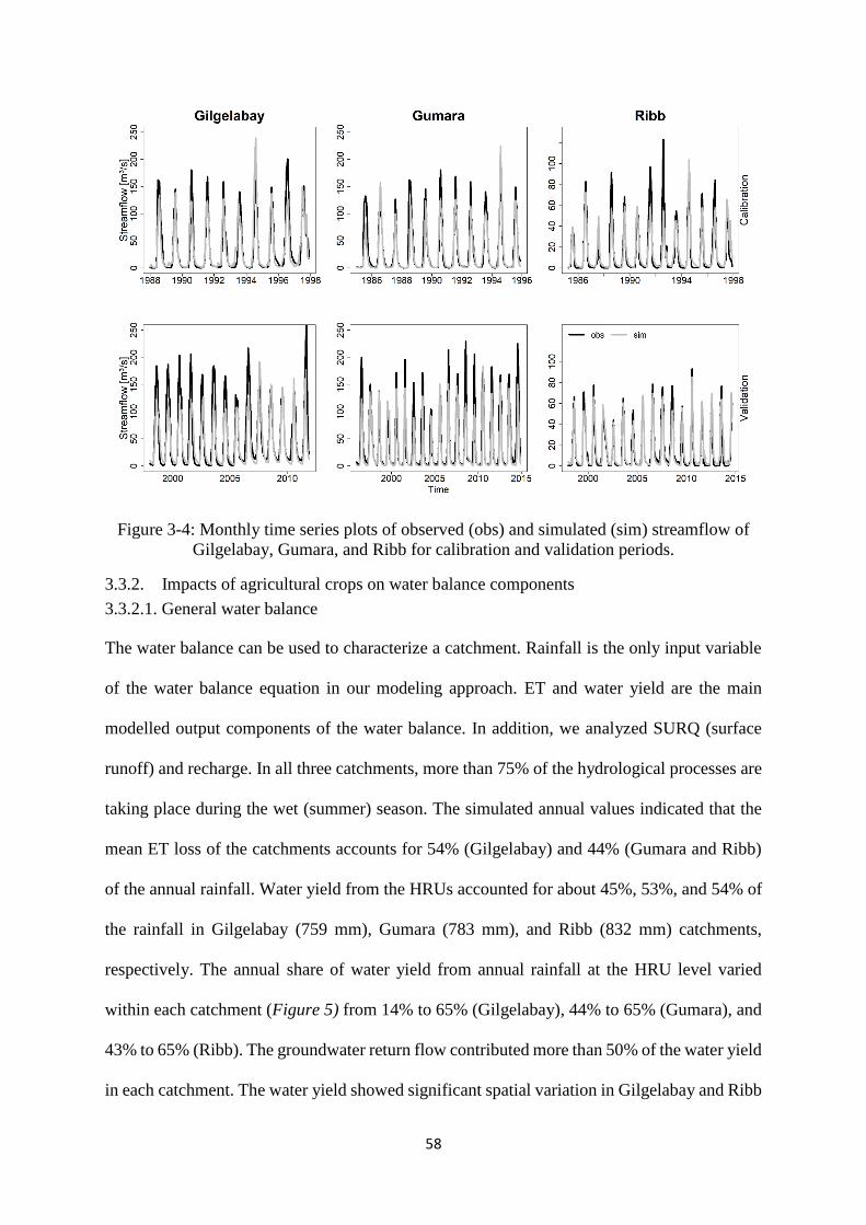
58
Figure 3-4: Monthly time series plots of observed (obs) and simulated (sim) streamflow of
Gilgelabay, Gumara, and Ribb for calibration and validation periods.
3.3.2. Impacts of agricultural crops on water balance components
3.3.2.1. General water balance
The water balance can be used to characterize a catchment. Rainfall is the only input variable
of the water balance equation in our modeling approach. ET and water yield are the main
modelled output components of the water balance. In addition, we analyzed SURQ (surface
runoff) and recharge. In all three catchments, more than 75% of the hydrological processes are
taking place during the wet (summer) season. The simulated annual values indicated that the
mean ET loss of the catchments accounts for 54% (Gilgelabay) and 44% (Gumara and Ribb)
of the annual rainfall. Water yield from the HRUs accounted for about 45%, 53%, and 54% of
the rainfall in Gilgelabay (759 mm), Gumara (783 mm), and Ribb (832 mm) catchments,
respectively. The annual share of water yield from annual rainfall at the HRU level varied
within each catchment (Figure 5) from 14% to 65% (Gilgelabay), 44% to 65% (Gumara), and
43% to 65% (Ribb). The groundwater return flow contributed more than 50% of the water yield
in each catchment. The water yield showed significant spatial variation in Gilgelabay and Ribb
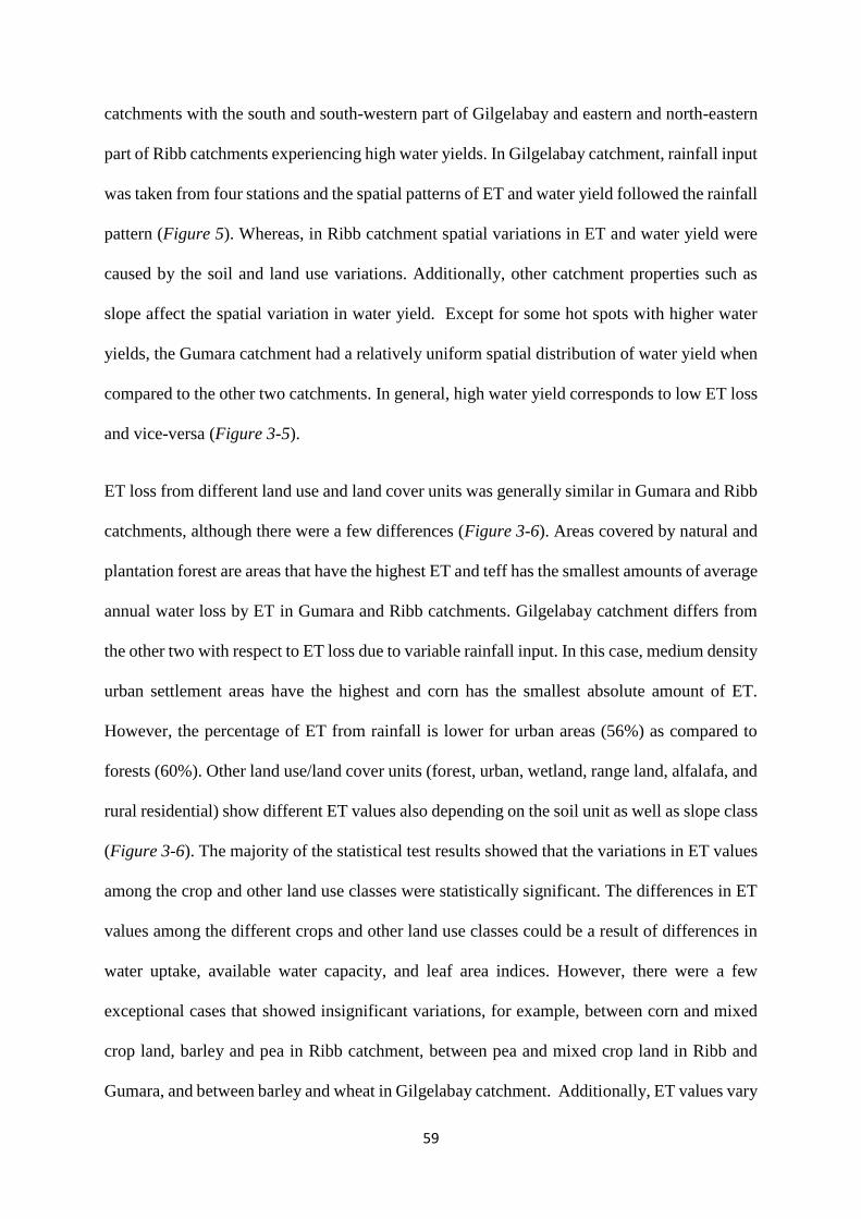
59
catchments with the south and south-western part of Gilgelabay and eastern and north-eastern
part of Ribb catchments experiencing high water yields. In Gilgelabay catchment, rainfall input
was taken from four stations and the spatial patterns of ET and water yield followed the rainfall
pattern (Figure 5). Whereas, in Ribb catchment spatial variations in ET and water yield were
caused by the soil and land use variations. Additionally, other catchment properties such as
slope affect the spatial variation in water yield. Except for some hot spots with higher water
yields, the Gumara catchment had a relatively uniform spatial distribution of water yield when
compared to the other two catchments. In general, high water yield corresponds to low ET loss
and vice-versa (Figure 3-5).
ET loss from different land use and land cover units was generally similar in Gumara and Ribb
catchments, although there were a few differences (Figure 3-6). Areas covered by natural and
plantation forest are areas that have the highest ET and teff has the smallest amounts of average
annual water loss by ET in Gumara and Ribb catchments. Gilgelabay catchment differs from
the other two with respect to ET loss due to variable rainfall input. In this case, medium density
urban settlement areas have the highest and corn has the smallest absolute amount of ET.
However, the percentage of ET from rainfall is lower for urban areas (56%) as compared to
forests (60%). Other land use/land cover units (forest, urban, wetland, range land, alfalafa, and
rural residential) show different ET values also depending on the soil unit as well as slope class
(Figure 3-6). The majority of the statistical test results showed that the variations in ET values
among the crop and other land use classes were statistically significant. The differences in ET
values among the different crops and other land use classes could be a result of differences in
water uptake, available water capacity, and leaf area indices. However, there were a few
exceptional cases that showed insignificant variations, for example, between corn and mixed
crop land, barley and pea in Ribb catchment, between pea and mixed crop land in Ribb and
Gumara, and between barley and wheat in Gilgelabay catchment. Additionally, ET values vary
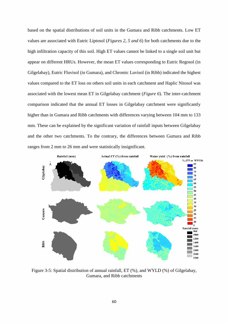
60
based on the spatial distributions of soil units in the Gumara and Ribb catchments. Low ET
values are associated with Eutric Liptosol (Figures 2, 5 and 6) for both catchments due to the
high infiltration capacity of this soil. High ET values cannot be linked to a single soil unit but
appear on different HRUs. However, the mean ET values corresponding to Eutric Regosol (in
Gilgelabay), Eutric Fluvisol (in Gumara), and Chromic Luvisol (in Ribb) indicated the highest
values compared to the ET loss on others soil units in each catchment and Haplic Nitosol was
associated with the lowest mean ET in Gilgelabay catchment (Figure 6). The inter-catchment
comparison indicated that the annual ET losses in Gilgelabay catchment were significantly
higher than in Gumara and Ribb catchments with differences varying between 104 mm to 133
mm. These can be explained by the significant variation of rainfall inputs between Gilgelabay
and the other two catchments. To the contrary, the differences between Gumara and Ribb
ranges from 2 mm to 26 mm and were statistically insignificant.
Figure 3-5: Spatial distribution of annual rainfall, ET (%), and WYLD (%) of Gilgelabay,
Gumara, and Ribb catchments

61
Figure 3-6: Boxplots showing the annual mean actual ET of HRUs for different land use/land
cover and soil units of Gilgelabay (first row), Gumara (second row), and Ribb (third row)
catchments
3.3.2.2. Runoff analyses
Surface runoff varied considerably in time and space in the study catchments (Figure 7). In all
three catchments about 90% of the total surface runoff was generated during the summer
months and the remaining 10% occurred during the other 8 months. The runoff coefficients
varied spatially among and within the three catchments due to changes in LULC and rainfall.
The annual runoff coefficients (the ratio of total streamflow to rainfall) were 0.32, 0.43, and
0.46 in Gilgelabay, Gumara, and Ribb, respectively. The variability of surface runoff was
linked to the LULC, soil type, topography of the area, as well as the associated model parameter
values. HRUs covered by medium density urban settlements, farm settlements, and mixed
cropland areas had a strong effect on increasing the magnitude of surface runoff. In the
Gilgelabay catchment, the mean annual surface runoff of HRUs decreased from farm village,
corn, mixed cropland, wheat, millet, barley, teff, permanent wetland, seasonal wetland, alfalfa,
and range grassland to evergreen forest. Differences among some agricultural crops and other
LULC classes were significant. For example, the changes between corn and other land use and
crop classes (forest, wetland, grassland, millet, barley, wheat and teff) vary from 14 mm to 83
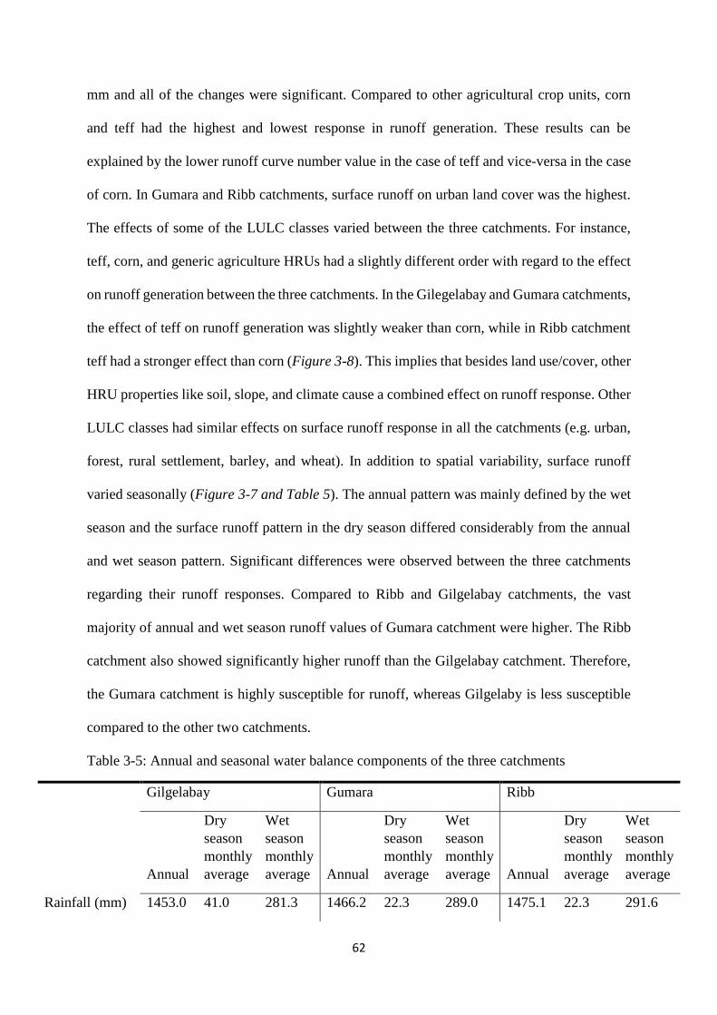
62
mm and all of the changes were significant. Compared to other agricultural crop units, corn
and teff had the highest and lowest response in runoff generation. These results can be
explained by the lower runoff curve number value in the case of teff and vice-versa in the case
of corn. In Gumara and Ribb catchments, surface runoff on urban land cover was the highest.
The effects of some of the LULC classes varied between the three catchments. For instance,
teff, corn, and generic agriculture HRUs had a slightly different order with regard to the effect
on runoff generation between the three catchments. In the Gilegelabay and Gumara catchments,
the effect of teff on runoff generation was slightly weaker than corn, while in Ribb catchment
teff had a stronger effect than corn (Figure 3-8). This implies that besides land use/cover, other
HRU properties like soil, slope, and climate cause a combined effect on runoff response. Other
LULC classes had similar effects on surface runoff response in all the catchments (e.g. urban,
forest, rural settlement, barley, and wheat). In addition to spatial variability, surface runoff
varied seasonally (Figure 3-7 and Table 5). The annual pattern was mainly defined by the wet
season and the surface runoff pattern in the dry season differed considerably from the annual
and wet season pattern. Significant differences were observed between the three catchments
regarding their runoff responses. Compared to Ribb and Gilgelabay catchments, the vast
majority of annual and wet season runoff values of Gumara catchment were higher. The Ribb
catchment also showed significantly higher runoff than the Gilgelabay catchment. Therefore,
the Gumara catchment is highly susceptible for runoff, whereas Gilgelaby is less susceptible
compared to the other two catchments.
Table 3-5: Annual and seasonal water balance components of the three catchments
Gilgelabay Gumara Ribb
Annual
Dry
season
monthly
average
Wet
season
monthly
average Annual
Dry
season
monthly
average
Wet
season
monthly
average Annual
Dry
season
monthly
average
Wet
season
monthly
average
Rainfall (mm) 1453.0 41.0 281.3 1466.2 22.3 289.0 1475.1 22.3 291.6
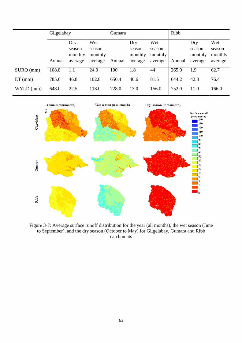
63
Gilgelabay Gumara Ribb
Annual
Dry
season
monthly
average
Wet
season
monthly
average Annual
Dry
season
monthly
average
Wet
season
monthly
average Annual
Dry
season
monthly
average
Wet
season
monthly
average
SURQ (mm) 108.8 1.1 24.9 190 1.8 44 265.9 1.9 62.7
ET (mm) 785.6 46.8 102.8 650.4 40.6 81.5 644.2 42.3 76.4
WYLD (mm) 648.0 22.5 118.0 728.0 13.0 156.0 752.0 11.0 166.0
Figure 3-7: Average surface runoff distribution for the year (all months), the wet season (June
to September), and the dry season (October to May) for Gilgelabay, Gumara and Ribb
catchments
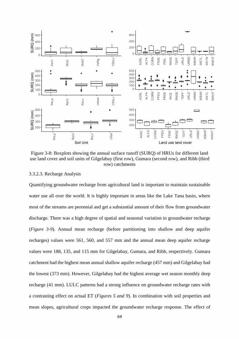
64
Figure 3-8: Boxplots showing the annual surface runoff (SURQ) of HRUs for different land
use land cover and soil units of Gilgelabay (first row), Gumara (second row), and Ribb (third
row) catchments
3.3.2.3. Recharge Analysis
Quantifying groundwater recharge from agricultural land is important to maintain sustainable
water use all over the world. It is highly important in areas like the Lake Tana basin, where
most of the streams are perennial and get a substantial amount of their flow from groundwater
discharge. There was a high degree of spatial and seasonal variation in groundwater recharge
(Figure 3-9). Annual mean recharge (before partitioning into shallow and deep aquifer
recharges) values were 561, 560, and 557 mm and the annual mean deep aquifer recharge
values were 188, 135, and 115 mm for Gilgelabay, Gumara, and Ribb, respectively. Gumara
catchment had the highest mean annual shallow aquifer recharge (457 mm) and Gilgelabay had
the lowest (373 mm). However, Gilgelabay had the highest average wet season monthly deep
recharge (41 mm). LULC patterns had a strong influence on groundwater recharge rates with
a contrasting effect on actual ET (Figures 5 and 9). In combination with soil properties and
mean slopes, agricultural crops impacted the groundwater recharge response. The effect of
65
LULC classes on groundwater recharge varied between the three catchments. In the Gilgelabay
catchment, millet and corn had the highest and second highest recharge rates. However, the
ranking differed in terms of volumetric contribution. Nearly 50% of the total wet months
recharge volume was contributed from corn- and teff-HRUs (corn, 29% and teff, 20%) as they
covered a larger portion of the catchment (Table 1). These are mostly found in the south-
western and western parts of the catchment that receive high amounts of rainfall (Figure 3-5
and 9). To the contrary, corn was among the LULC classes that had a low recharge rate in the
case of Gumara (Figure 3-10). This indicated that other catchment properties also played a role
in influencing recharge rates. In the Ribb catchment, agricultural areas covered by teff had the
highest average annual (614 mm) recharge to the shallow aquifer. Urban areas had the lowest
groundwater recharge in both Gumara and Ribb catchments (Figure 3-10). For the Gilgelabay
catchment, the mean annual groundwater recharge in medium density urban areas was higher
compared to other land uses due to the highest rainfall input, but its percent share of rainfall
was the lowest of all LULC classes (26%). For other LULC, 28% to 44% of the rainfall
recharged the shallow aquifer. As a whole, our statistical test results indicated that there were
significant variations in the rates of recharge among the different agricultural crops and other
LULC classes between and within the three catchments. Therefore, our initial hypothetical
assumption (no significance changes on the recharge rates among different land cover units)
was rejected. For example, the recharge rates of forest areas were significantly lower than the
recharge rates of agricultural areas (teff, barley, wheat, etc.) for all the three catchments.
Comparing recharge rates among the agricultural crop units showed that cereal crops (barley,
corn, rice, teff, and wheat) had significantly higher recharge rates than leguminous (pea) and
mixed cereal crop units. In addition to the LULC, the impact of soil units on recharge rate was
obvious in all catchments. Areas covered by Eutric Regosols and Eutric Leptosols were
identified as high groundwater recharge areas. In Gilgelabay catchment, areas covered by
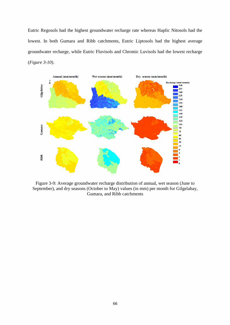
66
Eutric Regosols had the highest groundwater recharge rate whereas Haplic Nitosols had the
lowest. In both Gumara and Ribb catchments, Eutric Liptosols had the highest average
groundwater recharge, while Eutric Fluvisols and Chromic Luvisols had the lowest recharge
(Figure 3-10).
Figure 3-9: Average groundwater recharge distribution of annual, wet season (June to
September), and dry seasons (October to May) values (in mm) per month for Gilgelabay,
Gumara, and Ribb catchments
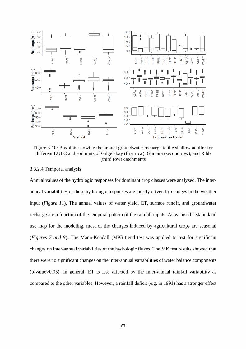
67
Figure 3-10: Boxplots showing the annual groundwater recharge to the shallow aquifer for
different LULC and soil units of Gilgelabay (first row), Gumara (second row), and Ribb
(third row) catchments
3.3.2.4.Temporal analysis
Annual values of the hydrologic responses for dominant crop classes were analyzed. The inter-
annual variabilities of these hydrologic responses are mostly driven by changes in the weather
input (Figure 11). The annual values of water yield, ET, surface runoff, and groundwater
recharge are a function of the temporal pattern of the rainfall inputs. As we used a static land
use map for the modeling, most of the changes induced by agricultural crops are seasonal
(Figures 7 and 9). The Mann-Kendall (MK) trend test was applied to test for significant
changes on inter-annual variabilities of the hydrologic fluxes. The MK test results showed that
there were no significant changes on the inter-annual variabilities of water balance components
(p-value>0.05). In general, ET is less affected by the inter-annual rainfall variability as
compared to the other variables. However, a rainfall deficit (e.g. in 1991) has a stronger effect
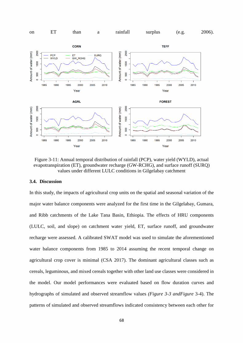
68
on ET than a rainfall surplus (e.g. 2006).
Figure 3-11: Annual temporal distribution of rainfall (PCP), water yield (WYLD), actual
evapotranspiration (ET), groundwater recharge (GW-RCHG), and surface runoff (SURQ)
values under different LULC conditions in Gilgelabay catchment
3.4. Discussion
In this study, the impacts of agricultural crop units on the spatial and seasonal variation of the
major water balance components were analyzed for the first time in the Gilgelabay, Gumara,
and Ribb catchments of the Lake Tana Basin, Ethiopia. The effects of HRU components
(LULC, soil, and slope) on catchment water yield, ET, surface runoff, and groundwater
recharge were assessed. A calibrated SWAT model was used to simulate the aforementioned
water balance components from 1985 to 2014 assuming the recent temporal change on
agricultural crop cover is minimal (CSA 2017). The dominant agricultural classes such as
cereals, leguminous, and mixed cereals together with other land use classes were considered in
the model. Our model performances were evaluated based on flow duration curves and
hydrographs of simulated and observed streamflow values (Figure 3-3 andFigure 3-4). The
patterns of simulated and observed streamflows indicated consistency between each other for
69
both calibration and validation periods. However, there are slight differences on the statistics
of the model efficiencies reflecting the temporal dynamics of streamflow data (Fohrer et al.,
2002). The model efficiencies were comparable with results of Setegn et al. (2008) and
Woldesenbet et al. (2017). However, our analysis of the flow duration curves indicates that
there is a disparity between the measured and modelled high flows (between 5% to 20%
exceedance probabilities with an RSR value 1.41) in the Gilgelabay catchment. This disparity
on the high flow segment might be linked to the limitation of the curve number method, as the
SCS-curve number method used in the SWAT model does not consider the duration and
intensity of rainfall (Nie et al. 2011, Woldesenbet et al. 2017). The Nash-Sutcliffe Efficiency
(NSE) for Gilgelabay catchment showed the lowest performance (0.53) compared to the other
two catchments (Table 4), which also pointed to the disparity on the high flow segment of the
FDC as NSE is known to give higher weights to high flows than to low flows (Guse et al.
2017). The underestimation of high flows can, to a lesser extent, be seen in the FDC for
Gumara, whereas the FDC for the Ribb catchment indicates a much closer match.
The spatial and seasonal distribution of the modelled hydrological components groundwater
recharge, surface runoff, water yield, and ET was analyzed. However, an independent
validation of the spatial distribution of ET and water yield was not possible due to a lack of
measured data. The accuracy of the derived patterns of ET and water yield relies on the model
validity, which was tested with measured streamflow data at the catchment outlet using a multi-
metric approach and flow duration curves. In addition, the seasonal development of the leaf
area index was checked for all land use classes to provide further confidence in the model
calculation. In our study, the Hargreaves method (Hargreaves and Samani 1985) was used to
compute potential evapotranspiration, which has been applied in several SWAT model studies
in Africa (e.g, Setegn et al. 2008; Notter et al. 2012; Woldesenbet et al. 2017). In addition,
Odusanya et al. (2019) compared the Hargreaves, the Penman–Monteith, and the Priestley–
70
Taylor method in SWAT for a catchment in Nigeria, and found that the ET values computed
using the Hargreaves method showed good agreement with satellite based ET patterns. These
studies provide further confidence in the accuracy of the derived ET patterns.
Likewise, the validity of the simulated surface runoff and groundwater recharge were not
verified independently. However, model outputs of the current study were compared to similar
studies in the region. In this study, the runoff coefficients calculated from the simulated
discharge were 0.32, 0.43, and 0.46 for Gilgelabay, Gumara, and Ribb, respectively. A study
conducted on the effects of the floodplain on river discharges into Lake Tana by Dissie et al.
(2014) reported that the runoff coefficient in the upper catchments of the Lake Tana basin vary
between 0.23 and 0.81 with an average value of 0.5. The simulated runoff coefficients from
our study are within this range. Furthermore, the ratios of average surface runoff to total
streamflow found in our study were 0.23, 0.28, and 0.35 for Gilgelabay, Gumara, and Ribb,
respectively. In support of these values are the findings by Jemberie et al. (2016), who reported
that the average surface runoff to total streamflow ratio of the Lake Tana basin is 0.28.
In this study, the modelled water balance components showed a high degree of variation in
their spatial and seasonal distribution. These spatial variations are due to variations in land use
and land cover types, soil permeability and porosity, and slope class of the area, as well as
varying climatic input data. The seasonal variations are induced due to the temporal variation
of rainfall and variation in the canopy coverage of the different crops during the wet and dry
seasons. The water balance analysis indicates that different HRU components (LULC/crop,
soil, and slope classes) do not equally affect the catchment’s hydrology. The influence of slope
is smaller when compared to soil and crop types. When the groundwater recharge and surface
runoff generation were analyzed for different slope classes under the same land use (teff) and
soil (Eutric Liptosol), the observed variation was about 1%. To the contrary, the groundwater
recharge and surface runoff showed significant variations (from 47% to 50%) when Eutric
71
Liptosols is changed to Haplic Luvisols for an HRU with teff and foot slope. Thus, variations
in vegetation and soil types have a higher influence than slope in our simulation results. The
changes in the water balance components were also significant between different agricultural
crop units. Similarly, Li et al. (2019) reported a substantial impact on the hydrology of Wei
River basin due to expansion of cropland. As an example, in the Gumara and Ribb catchments,
the groundwater recharge over time in areas covered by teff was significantly higher than the
groundwater recharge in areas covered by other agricultural crops. In the Gilgelabay
catchment, HRUs with agricultural area covered by millet have the highest average
groundwater recharge followed by agricultural land covered by corn. These higher recharge
rates on teff and millet crop cover areas might be linked to the lower water demand for
evaporation as the water interception capacity and leaf area index values are lower than in other
LULC units like forest and shrub lands. Moreover, forest cover and shrub land areas had less
recharge compared to cropland because a larger amount of water was evapotranspirated. The
results are in agreement with the findings of Nie et al. (2011) who studied the impact of land
use and land cover change on the hydrology of the upper San Pedro watershed. Their scenario-
based simulation indicated that the baseflow/percolation decreased when grassland was
replaced by shrub land. A study by Gumindoga et al. (2014) on predicting streamflow for land
cover changes in the Gilgelabay catchment also reported a higher groundwater recharge on
agricultural areas than forest areas. Their findings are in agreement with the current study. The
other crop types also exhibit different recharge rates based on the daily water needs and the
phenological stage. Cereal crops like millet, teff, wheat, and barley show relatively good
recharge due to less water interception and transpiration demand even in a full development
stage when compared to mixed crops, pulses, and rice. Our results are in agreement with
research findings of Fohrer et al. (2001) who reported that the baseflow was increased for an
area covered with barley compared to forest cover due to the lower water interception capacity
72
of barley in Germany. Therefore, it can be concluded that cereal crops such as teff, barley,
wheat, and millet enhanced the groundwater recharge by reducing ET and surface runoff in the
three catchments. Additionally, our runoff analysis results indicated that agricultural crops such
as pea increased runoff when compared to other agricultural crop classes. Hence, an expansion
of agricultural crops like pea affects the water availability in the region, which should be
considered during decision making processes.
The spatial dynamics of the hydrologic components for Gilgelabay catchment showed similar
patterns to the differing rainfall input. The sub-basins located on the southern and southwestern
part of the catchment have the highest amount of rainfall and are characterized as a high
groundwater recharge and surface runoff zone (Figure 3-5, 7, and Figure 3-9). This part of the
catchment which accounts for about 15% of the total area has the highest runoff response due
to high rainfall intensity, steep slope classes, and Haplic Alisols. A secondary clay minerals
assemblage domination is a typical feature of Haplic Alisols, which could a cause high runoff
response (IUSS Working Group WRB 2015). In the Gumara and Ribb catchments only one
rainfall station was used, so that LULC and soil units have more influence on the spatial
patterns of hydrologic components than rainfall. There is a high degree of spatial variability of
the hydrological processes as the soil units change from Eutric Leptosols (mainly dominated
by gravel and sand, and belongs to hydrologic soil group B) to texturally clay dominated Eutric
Vertisols and Chromic Fluvisols, which belong to hydrologic soil group C and D, respectively.
The northern and southeastern parts of Gumara and Ribb catchments, which are covered by
Eutric Leptosols (hydrologic soil group B), are relatively good groundwater recharge zones.
The reason for this is that Eutric Leptosols are sand dominated and characterized by many
coarse fragment soil particles (IUSS Working Group WRB 2015). The highest amount of
surface runoff occurred on areas covered by Eutric Fluvisols (hydrologic soil group D). Thus,
soil class boundaries are good benchmarks to map groundwater recharge zones in the
73
catchments (Figure 9). With respect to LULC, agricultural areas covered by teff and wheat
have the highest groundwater recharge potential due to their low leaf area index, which allows
for more infiltration. Low density rural settlement areas are characterized by the lowest
groundwater recharge and highest surface runoff. The higher surface runoff which is seen in
settlement areas due to impervious surfaces is well supported by the literature: Zhang et al.
(2016), who studied hydrological responses to land use change scenarios under constant and
changed climatic conditions of the Heihe River basin, China, reported that developed lands
produced higher runoff than cultivated and grassland and Wagner et al. (2016) linked an
increase in urban area to an increase in water yield on the sub-basin level in a meso-scale
catchment in India and, the increase in runoff to the onset of monsoon (Wagner et al. 2016).
The absolute values of ET decreased from forest cover to cultivated land for all three
catchments due to the high canopy storage, leaf area index, and transpiration demand for forest
cover compared to cropland (Nie et al., 2011). In the case of the Gilgelaby catchment, urban
and rural settlements have the highest average annual actual evapotranspiration due to high
rainfall input. However, their percentage shares from the total rainfall (urban, 40% and rural
settlements, 56%) are still less than forest (60%) (Figure 6).
The overall mean annual ET loss from annual rainfall accounts for 54% in Gilgelabay and for
44% in Gumara and Ribb. Setegn et al. (2008) reported that more than 60% water is lost as ET.
This variation could be due to the differences in the model setups and periods of simulation, as
well as variation of the LULC data that were used. Setegn et al. (2008) used a single SWAT
model for the whole Lake Tana Basin with 10%, 20%, and 10% threshold values of LULC,
soil, and slope, respectively, whereas the current study was carried out by setting up three
independent models for Gilgelabay, Gumara, and Ribb catchments using highly refined LULC
data (with no threshold limit for LULC, soil, and slope). Our findings showed significant
dynamics of the hydrologic components between the wet and dry seasons. More than 90% of
74
the groundwater recharge and surface runoff and about 49% of the ET took place during the
wet season. This implies that the influence of rainfall for the hydrologic processes in the region
is significant. The total streamflow values are dominated by the baseflow in all the three
catchments (73%, 62%, and 60% of the total streamflow in Gilgelabay, Gumara, and Ribb,
respectively). Setegn et al. (2008) reported a value of 59% for the Gilgelabay catchment. The
higher baseflow contribution for the Gilgelabay catchment in this study may be due to the
higher fitted values of SURLAG and ALPHA_BF, which affect the runoff and baseflow
response. Moreover, baseflow is a function of catchment area, and geomorphological,
geological, and hydrogeological parameters of the catchment (Wosenie et al. 2014). In this
study, the effect of catchment area on baseflow contribution was reflected. The Gilgelabay
catchment, which is the largest of the three, had the highest baseflow contribution, whereas the
Ribb catchment, which is the smallest catchment, had the lowest baseflow contribution to
streamflow. The annual deep groundwater recharge accounts for 13%, 9%, and 7% of annual
rainfall for Gilgelabay, Gumara, and Ribb, respectively. The order of the amount of deep
groundwater recharge is in agreement with the order of the fitted values for RCHRG_DP in
our model (Table 3). These results are in line with Wosenie et al. (2014) who reported that the
Gilgelabay catchment had higher groundwater recharge rates than the Gumara catchment.
3.5. Summary and conclusion
In this study, the impacts of agricultural crops and other LULC classes on the major water
balance components were investigated in the Gilgelabay, Gumara, and Ribb catchment, Lake
Tana basin, Ethiopia.
Our findings show that the spatial and seasonal values of ET in the Gilgelabay catchment were
significantly different from the values in Gumara and Ribb. Likewise, the groundwater
recharge and surface runoff values revealed significant spatial and seasonal variations between
the three catchments. To the contrary, the ET values between Gumara and Ribb catchments
75
showed insignificant variations. Compared to Gilgelabay and Ribb, the Gumara catchment
showed high susceptibility for runoff, whereas Gilgelaby is less susceptible compared to the
other two catchments. Besides, the results showed that there were no significant differences in
the inter-annual variabilities of ET, surface runoff, water yield, and groundwater recharge.
In summary, our findings highlight the significance of considering agricultural crop classes in
the application of hydrologic models, which often rely on only one generic agricultural class.
The vast majority of the agricultural crop classes had a significant effect on the water balance
components. On the one hand, cereal crops had higher rates of groundwater recharge compared
to others like leguminous and mixed crops. On the other hand, leguminous crops like peas had
significant impact on increasing runoff generation. Therefore, expansion of agricultural crops
like pea may be discouraged as they favoured surface runoff generation, which in turn may
lead to a higher erosion risk. In this regard, the present research approach could be extrapolated
to similar catchments in Ethiopia and other African countries where agricultural land use
dominates.
Moreover, for future impact assessment of agricultural crops on water balance components, a
time series LULC could provide further insights into inter-annual impacts on the water
resources. In addition, it is recommended to incorporate climate change in future assessments
of groundwater and surface water dynamics to derive sustainable solutions for the future.
76
4. Modeling spatio-temporal flow dynamics of groundwater-surface water
interactions of the Lake Tana Basin, Upper Blue Nile, Ethiopia
*Tibebe B. Tigabu, Paul D. Wagner, Georg Hörmann and Nicola Fohrer
Department of Hydrology and Water Resources Management, Institute for Natural Resource
Conservation, Kiel University, D-24118 Kiel, Germany
Address to correspondence author: Tibebe Tigabu, Department of Hydrology and Water
Resources Management, Institute of Natural Resource Conservation, CAU, D-24118 Kiel,
Germany, E-mail: [email protected]
Hydrological Research (2020):
Submitted: 13 January 2020 – Under revision: since 13 January 2020
77
Abstract
The Ethiopian government has selected Lake Tana basin as a development corridor due to its
groundwater (GW) and surface water (SW) potential. However, there is little knowledge about
the flow dynamics of GW and SW in the Lake Tana basin, Ethiopia. Mostly, water from the
aquifer system is extracted in an unplanned and unregulated manner that could result in over-
pumping of the aquifer system. Therefore, this study aims to investigate the flow dynamics of
GW-SW systems on a spatio-temporal basis and to assess if there is a hydraulic connection
between GW and SW systems in three of the main catchments (Gilgelabay, Gumara and Ribb)
that drain into Lake Tana. The SWAT-MODFLOW model, which is an integration of SWAT
(Soil and Water assessment Tool) and MODFLOW, is used as a hydrologic model with coupled
surface and sub-surface flow is necessary to investigate GW-SW interactions. The results
reveal that aquifer and the stream network systems are hydraulically connected to each other
in all three catchments. In the Gilgelabay catchment the flow from the aquifer to the river cells
dominates, whereas in Gumara and Ribb, the main flow is from the river cells to the aquifer
system. The daily GW-SW interaction rate is more dynamic than the annual one. Moreover,
the flow pattern differs in the three catchments due to spatial variations of the aquifer
parameters and morphological heterogeneity among the catchments. The average groundwater
recharge to the MODFLOW grid cell shows high seasonal variation in all three catchments.
For instance, in the Gumara catchment, the mean annual groundwater recharge to the
MODFLOW grid cell is about 80 m³/day, whereas the wet season mean is about 220 m³/day,
and the dry season mean is only 20 m³/day.
Keywords: Coupling, flow dynamics, groundwater-surface water interaction, SWAT-MODFLOW,
hydraulic head, spatio-temporal, seasonal variation, and recharge
78
4.1. Introduction
Water availability and water quality are main challenges of the 21st century due to a growing
water demand. The challenge is twofold for developing countries like Ethiopia because of a
limitation in technology and financial resources to invest in water resources development.
Thus, groundwater (GW) is the only reliable water supply option for most rural areas in Africa
to meet the dispersed demand (Hiscock 2011). However, mostly extraction of water from the
aquifer system is not planned and or regulated, so that it could result in over-pumping of the
aquifer system. Therefore, a comprehensive understanding of watershed hydrology with
particular emphasis on the interaction of GW and surface water (SW) is essential for sustainable
water management in a watershed (Bailey et al. 2016).
So far, several studies have focused on modelling GW and SW interactions; Jayasekera et al.
(2011) studied GW stress and vulnerability in rural coastal aquifers using an empirical model
known as modified DRASTIC (Depth to the GW table, net GW Recharge, Aquifer media, Soil
media, Topography, Impact of vadose zone media, and hydraulic Conductivity of the aquifer).
Sutanudjaja et al. (2011) had constructed a large scale MODFLOW transient GW model
coupled with a distributed land surface model for the Rhine-Meuse basin based on readily
available global datasets. Ahring and Steward (2012) studied the GW-SW interaction using the
spatial distribution of phreatophytes. Pfannerstill et al. (2014) investigated GW processes in a
German lowland catchment and improved their representation in the SWAT model. Duvert et
al. (2015) analyzed the variability of GW within the aquifer system and assessed the response
of the aquifer system to high and low frequency rainfall variations. Goderniaux et al. (2015)
studied the uncertainty of climate change impact on GW reserves, and Gemitzi et al. (2017)
developed an empirical monthly GW recharge equation based on modelling and remote sensing
data to predict potential climate change impacts.
79
Moreover, strong efforts have been conducted to integrate SWAT (Soil and Water Assessment
Tool) (Arnold et al. 1998) and MODFLOW (Harbaugh et al. 2000) to analyse GW and SW
interactions. For example, Guzman et al. (2015) developed an integrated SWAT and
MODFLOW model (“SWATmf”) to improve the assessment of impacts of natural and
anthropogenic stressors on both SW and GW resources at the watershed scale, and Izady et al.
(2015) applied the combined SWAT-MODFLOW model to estimate GW recharge for a
catchment located in northeast of Iran. Bailey et al. (2016) developed the coupled SWAT-
MODFLOW model, that was upgraded later into the graphical user interface model
SWATMOD-Prep (Bailey et al. 2017). Ehtiat et al. (2018) integrated SWAT, MODFLOW,
and MT3DMS to investigate how SW conditions affect the quality of the GW system in a non-
coastal aquifer. Chunn et al. (2019) studied the impacts of climate change and water withdrawal
on the GW-SW interactions in West-Central Alberta using the integrated SWAT-MODFLOW
model. Similarly, Park et al. (2019) developed a QGIS-based graphical user interface SWAT-
MODFLOW model for Middle Bosque River Watershed in central Texas. However, as
compared to the number of catchment modelling studies and their regional coverage, more
efforts are needed to assess GW-SW interaction in different parts of the world.
Ethiopia is one of those regions where GW resources are under severe pressure and widely
used even though the system is not yet well understood. In the Lake Tana basin, low flows are
expected to decline by up to -61% under the A1B and B1 emission scenarios for 2050s (Taye
et al. 2015). Consequently, it is assumed that more GW will be used to overcome the freshwater
constraint in Ethiopia in general and in the Lake Tana Basin in particular. According to the
Ethiopian government growth and transformation plan, agriculture irrigated from GW sources
is expected to cover 2 million hectare by 2020 (Kebede 2012). Due to its proximity to the point
of demand, GW provides 90% of the domestic water supply, 95% of the industrial use, and a
small proportion of irrigation water demand. In general, 80% of the total national water supply
80
comes from GW (Kebede 2018). Previous hydrological studies focused on the surface water
use and hydrologic balance and do not adequately address issues of GW, particularly in the
context of combining SW–GW models in the Lake Tana Basin. For example, Setegn et al.
(2008) applied SWAT2005 to model the hydrologic balance of the Lake Tana Basin with the
main objective to test the performance and feasibility of SWAT model in predicting streamflow
in the basin; Seyoum et al. (2013) used a flow forecasting model (HEC–HMS) for their rainfall-
runoff prediction in Gumara and Ribb catchments; Gebremicael et al. (2013) investigated the
long-term variability of rainfall, runoff and sediment fluxes, and causes of changes in runoff
and sediment load of the Upper Blue Nile; Dessie et al. (2015) anaylyzed the daily water blance
of the Lake Tana using a simple rainfall-runoff model; Worqlul et al. (2015) studied the
availability of surface water for irrigation use; Dile et al. (2016) focused on the implications
of water harvesting intensification on upstream–downstream ecosystem services of the Lake
Tana Basin, and Woldesenbet et al. (2017) focused on land use/cover change impact on
hydrologic responses of the Lake Tana and Beles sub-basins. Conway & Hulme (1996)
reported that there is high SW stress in the Upper Blue Nile region over time due to global
warming. Because of the SW stress, nowadays the Ethiopian government focuses on using
more GW for different purposes than before (MoW 2011). A recent study conducted by
Woldesenbet et al. (2017) revealed that the average annual baseflow and percolation decreased
gradually, to the contrary the average annual surface runoff increased due to land use and land
cover changes of Tana and Beles sub-basins in Ethiopia between 1986 and 2010. Dile et al.
(2018) reviewed hydrological research papers that have been focusing on the Upper Blue Nile
basin and they recommended that future research shall focus on the application of coupled
models to predict multiple outcomes across multiple spatial and temporal scales in the basin as
most of the previous studies have been focused on single model applications to estimate a single
output such as streamflow or sediment loss at the outlet of a catchment. Chebud and Melesse
81
(2009) applied a numerical model to investigate the groundwater flow system in the Gumara
catchment and they identified that there is a research gap on the spatial and temporal
distribution of percolation in the Gumara catchment in particular, and in Lake Tana Basin in
general. A hydrologic modelling study that applied the SWAT model in the catchments of
Gilgelabay, Gumara, and Ribb showed that the flow systems are strongly influenced by GW
(Tigabu et al. 2019). Therefore, the application of a coupled hydrologic model that is capable
of simulating SW and GW and their interaction is required in areas like the Lake Tana Basin,
which often lack piezometric information to characterize local GW and SW interactions.
Thus, we apply a coupled SWAT-MODFLOW model (SWAT: Arnold et al., 1998; Arnold &
Fohrer 2005; MODFLOW: Harbaugh 2005; coupling interface SWATMOD-Prep: Bailey et al.
2017) to enhance our understanding of the spatio-temporal interactions of GW and SW in the
Lake Tana basin, Upper Blue Nile, Ethiopia. The specific objectives of this study are:
to investigate if the aquifer and stream network systems are hydraulically connected,
to assess GW-SW exchange rates at river cell and sub-basin levels, and to identify the
spatial extent of GW discharge and recharge areas,
to determine if there are differences in GW-SW interactions between the three
catchments,
and to understand the spatial variability of the GW hydraulic head.
4.2. Materials and Methods
4.2.1. Study area
The Lake Tana basin, which is the second largest sub-basin of the Blue Nile, is situated in the
north-western part of Ethiopia (Figure 3-1). The catchment area of the basin at the outlet of
Lake Tana is 15,321 km2. The lake has a surface area of 3,156 km2 that covers about 20% of
the total catchment area (Alemayehu et al. 2010, Tigabu et al. 2018). The catchment has a very
82
diverse topography with an altitude ranging from 1322 m to 4111 m above sea level (Tigabu
et al. 2018). Moreover, the lake is shallow with a maximum depth of 15 m and characterized
by a steep slope at the borders and by a flat bottom (Kebede et al. 2006). It comprises about
50% of the country’s fresh water (Costa et al. 2014). The Blue Nile River originates from Lake
Tana. More than 40 rivers and streams flow into Lake Tana with a mean annual inflow of 158
m3/s (Alemayehu et al. 2010), but 86% of the water originates from three major rivers:
Gilgelabay, Gumara, and Ribb (Alemayehu et al. 2010). The annual volume of surface outflow
measured at the lake outlet is 4 billion m3 (Figure 3-1).
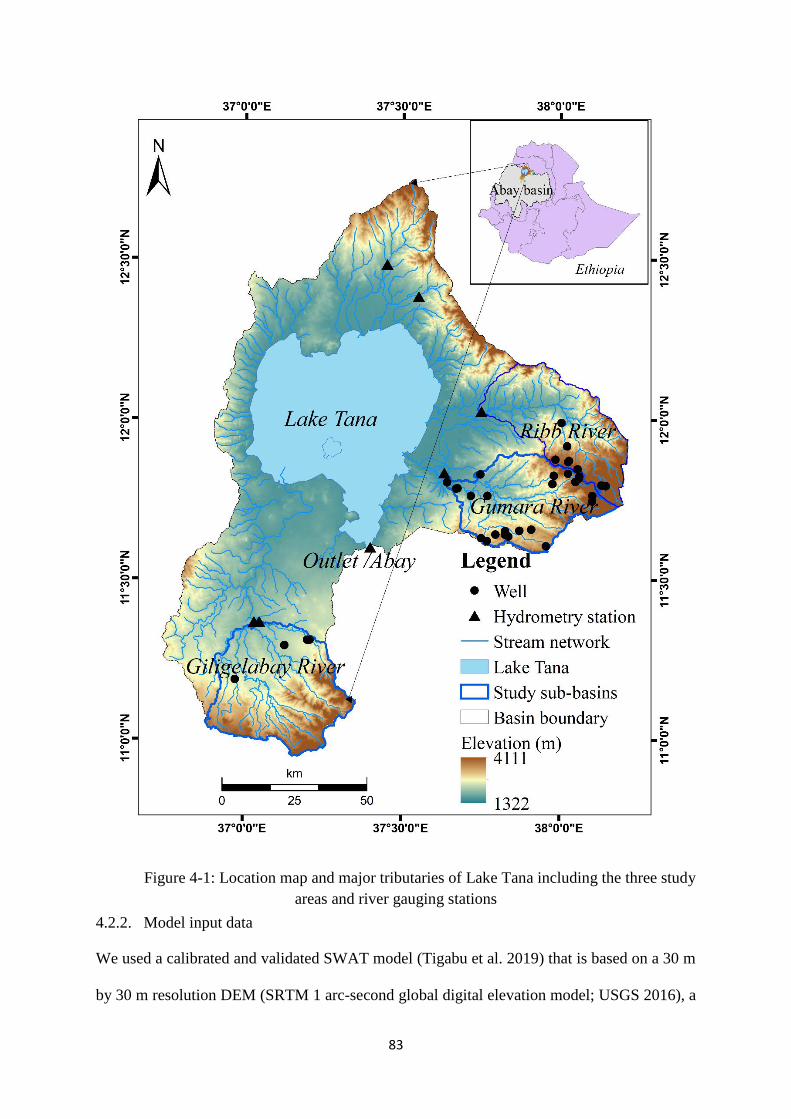
83
Figure 4-1: Location map and major tributaries of Lake Tana including the three study
areas and river gauging stations
4.2.2. Model input data
We used a calibrated and validated SWAT model (Tigabu et al. 2019) that is based on a 30 m
by 30 m resolution DEM (SRTM 1 arc-second global digital elevation model; USGS 2016), a
84
soil map and a land use map from the Amhara Design & Supervision Works Enterprise
(ADSWE 2017). Daily weather data including rainfall and maximum and minimum
temperature were available from the National Meteorological Service Agency (NMA 2016).
The SWAT model with its sub-basins, hydrologic response units (HRUs), and river network
shapefiles were inputs to the coupled SWATMOD-Prep model (Table 1). Moreover for the
parameterization of MODFLOW, maps of initial GW head were prepared by inverse distance
weighted (IDW) interpolation of water level data from hand-dug wells and boreholes that were
collected from Amhara Water Works Construction (AWWCE 2016) and Tana Basin
Development Authority (TBDA 2016). Saha et al. (2017) have applied the same approach in
their modelling study of temporal dynamics of groundwater-surface water interactions for a
watershed in Canada. Hydraulic conductivities, specific storage, and specific yield values were
assigned to each soil unit based on previously published values (Morris and Jonson 1967), and
river bed material K (default value of MODFLOW) were used as input data for the
MODFLOW model. The horizontal and vertical anisotropy factors for all materials were set to
1, assuming that these anisotropies were not changing both horizontally and vertically. The
streamflow data from gauging stations Gilgelabay near Merawi, Gumara near Bahirdar, and
Ribb near Addis Zemen for the years 1980 to 2014 were provided by the Ministry of Water,
Irrigation and Electricity of the Ethiopian Government (MoWIE 2016) to validate the coupled
model.
4.2.3. SWATMOD-Prep Setup
SWATMOD-Prep is a graphical user interface (Bailey et al. 2017), that was used to set up
coupled SWAT-MODFLOW models for the catchments of Gilgelabay (upper part), Gumara,
and Ribb (upper part) river that are part of the Lake Tana Basin. Each catchment was
discretized into finite different MODFLOW grid cells with a lateral dimension of 210 m by
210 m. The boundaries of the catchments were considered as boundary condition for active and
85
inactive cells. The rows and columns are oriented east-west and north-south, respectively. The
three catchments have a different number of rows and columns as their sizes vary. After the
MODFLOW grid cells are created, HRUs are disaggregated into DHRU that are individual,
contiguous areas within a sub-basin to allow HRU calculations to be geolocated (Bailey et al.
2017). The DHRUs and the MODFLOW grid cells were intersected, and river segments were
defined using polygons (called river cells) that were identified to pass data between SWAT and
MODFLOW. Then, SWAT-MODFLOW linkage files were written using subroutines of a three
dimensional finite difference subsurface flow model (MODFLOW-NWT) and subroutines
from SWAT (2012, Revision 664) to relate HRUs to MODFLOW grid cells and MODFLOW
river cells to SWAT stream channels (Bailey et al. 2016; Bailey et al. 2017). MODFLOW-
NWT was designed to simulate 3D subsurface flow such as GW recharge, GW discharge,
pumping, and interaction of GW-SW with the stream network (Harbaugh 2005). MODFLOW
models were created within the SWATMOD-Prep environment using the 30 m resolution
SRTM-DEM, aquifer thickness, GW head, hydraulic conductivities, specific storage and
specific yield (standard values were assigned based on geologic formations), and river bed
material K value. In this study, only the first unconfined layer of the aquifer system was
considered due to the limitation of SWAT-MODFLOW in modeling the aquifer system below
the first layer (Bailey et al. 2016). In the SWAT model, the first unconfined layer of the aquifer
system was assumed to be a layer right above the impervious layer (maximum 6 meter below
the surface) to the water table (Neitsch et al. 2011). The geologic log information from 36
drilled wells (AWWCE 2016) were used to determine the water table depth to the impervious
layer. The values vary between 0.5 to 12.5 m. We considered the average of the geologic log
information (6 m) as the average aquifer thickness in SWAT. The hydraulic head values from
the 36 boreholes were used as the initial conditions to simulate aquifer head values for each
MODFLOW grid cell under transient condition. Chebud and Melesse (2009) had used the same
86
kind of data for their MODFLOW modelling work in the Gumara catchment. Recharge data
from each HRU were taken directly from the calibrated SWAT model. Finally, SWAT-
MODFLOW simulations were carried out for the three catchments, and the spatial and
temporal interactions of GW and SW were evaluated for the three catchments. The River
package of MODFLOW was used to simulate the GW–SW interaction and the Darcy-equation
was used to calculate the volumetric flow of water through the cross-sectional flow area
between the aquifer and the stream channel (Bailey et al. 2016). Due to lack of documented
information on water withdrawal, pumping rates were not considered in the current study.
4.2.4. Simulation outputs
The model is capable to simulate the hydraulic head for each MODFLOW grid cell, deep
percolation (called recharge in SWAT-MODFLOW) for each HRU, volumetric exchange rates
(m3/day) between the stream network and the aquifer for each SWAT sub-basin and volumetric
exchange rate (m3/day) between the stream network and the aquifer for each MODFLOW River
cell. Our simulations for GW-SW interaction were carried out on a daily time step from 1985
to 2014 and the analyses focused on the monthly hydraulic head, GW-SW exchange, and GW
recharge. These outputs were extracted and processed using different R packages such as readr
(Wickham et al. 2017), stringr (Wickham 2018), dplyr (Wickman et al. 2018), and ggplot2
(Wickham 2011). Spatial distributions were produced by mapping the model output to the HRU
location. These maps presented the spatial extent of source and sink areas, the variation of the
hydraulic head, and GW recharge to MODFLOW. Moreover, temporal variations of GW-SW
interactions were shown with the help of time series plots for those sub-basins that include
gauging stations.
4.2.5. Model evaluation
To evaluate the performances of the coupled SWAT-MODFLOW models for the three
catchments, the simulated streamflow data were validated against the measured streamflow
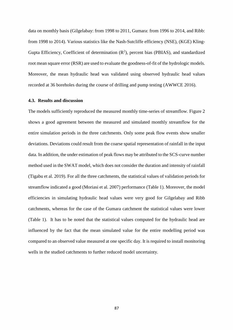
87
data on monthly basis (Gilgelabay: from 1998 to 2011, Gumara: from 1996 to 2014, and Ribb:
from 1998 to 2014). Various statistics like the Nash-Sutcliffe efficiency (NSE), (KGE) Kling-
Gupta Efficiency, Coefficient of determination (R2), percent bias (PBIAS), and standardized
root mean square error (RSR) are used to evaluate the goodness-of-fit of the hydrologic models.
Moreover, the mean hydraulic head was validated using observed hydraulic head values
recorded at 36 boreholes during the course of drilling and pump testing (AWWCE 2016).
4.3. Results and discussion
The models sufficiently reproduced the measured monthly time-series of streamflow. Figure 2
shows a good agreement between the measured and simulated monthly streamflow for the
entire simulation periods in the three catchments. Only some peak flow events show smaller
deviations. Deviations could result from the coarse spatial representation of rainfall in the input
data. In addition, the under estimation of peak flows may be attributed to the SCS-curve number
method used in the SWAT model, which does not consider the duration and intensity of rainfall
(Tigabu et al. 2019). For all the three catchments, the statistical values of validation periods for
streamflow indicated a good (Moriasi et al. 2007) performance (Table 1). Moreover, the model
efficiencies in simulating hydraulic head values were very good for Gilgelabay and Ribb
catchments, whereas for the case of the Gumara catchment the statistical values were lower
(Table 1). It has to be noted that the statistical values computed for the hydraulic head are
influenced by the fact that the mean simulated value for the entire modelling period was
compared to an observed value measured at one specific day. It is required to install monitoring
wells in the studied catchments to further reduced model uncertainty.
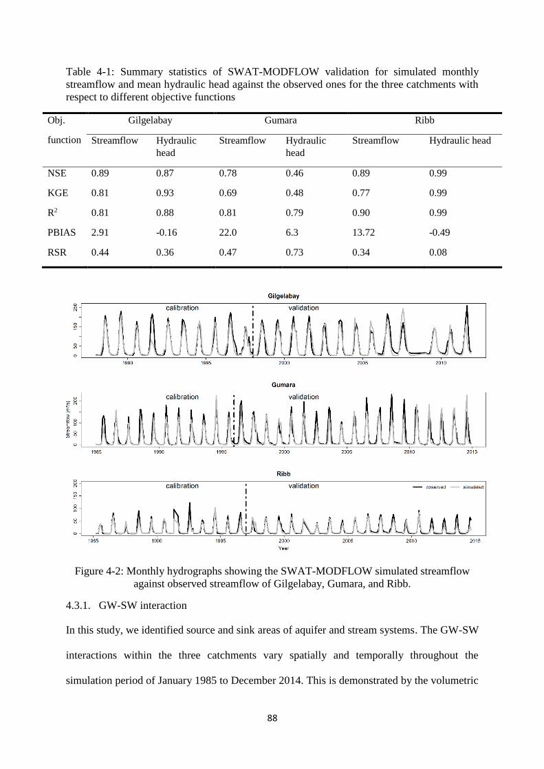
88
Table 4-1: Summary statistics of SWAT-MODFLOW validation for simulated monthly
streamflow and mean hydraulic head against the observed ones for the three catchments with
respect to different objective functions
Obj.
function
Gilgelabay Gumara Ribb
Streamflow Hydraulic
head
Streamflow Hydraulic
head
Streamflow Hydraulic head
NSE 0.89 0.87 0.78 0.46 0.89 0.99
KGE 0.81 0.93 0.69 0.48 0.77 0.99
R2 0.81 0.88 0.81 0.79 0.90 0.99
PBIAS 2.91 -0.16 22.0 6.3 13.72 -0.49
RSR 0.44 0.36 0.47 0.73 0.34 0.08
Figure 4-2: Monthly hydrographs showing the SWAT-MODFLOW simulated streamflow
against observed streamflow of Gilgelabay, Gumara, and Ribb.
4.3.1. GW-SW interaction
In this study, we identified source and sink areas of aquifer and stream systems. The GW-SW
interactions within the three catchments vary spatially and temporally throughout the
simulation period of January 1985 to December 2014. This is demonstrated by the volumetric
89
exchange rate (m3/day) between the stream network and the aquifer for each MODFLOW river
cell, and between the stream network and the aquifer for each SWAT sub-basin (Fig. 3, 4, and
5). In the highland areas, the stream systems are mainly a source for the aquifer indicating that
water is flowing from the river cell to the aquifer, and that the aquifer is a sink for the stream
system. The spatio-temporal variations in the GW-SW exchange rates depend on the head
difference between the aquifer and the stream and on the aquifer properties such as hydraulic
conductivity, specific storage and initial groundwater head (Kim et al. 2008).
In the Gilgelabay catchment, the long-term mean annual volumetric GW exchange rate for each
of the SWAT sub-basins is positive indicating that the aquifer system is a source area for the
streams systems. The net annual mean contribution from the aquifer to the stream network in
the sub-basin at the catchment outlet is 170 m3/day. However, the flow patterns are highly
dynamic on a monthly basis (Fig. 3). The time-series pattern of GW-SW interaction show
higher exchange rates during the wet months (July, August, September) and gradually diminish
for the rest of the months, which signifies the seasonal variations of aquifer heads. Kim et al.
(2008) found similar results to the Musimcheon Basin in Korea when they applied the
integrated SWAT-MODFLOW model to simulate spatio-temporal distribution of GW recharge
rates and GW evapotranspiration. Both, an exchange of water from the river network to the
aquifer and vice-versa can be observed. The latter especially occurs during rainy days
indicating that the water level of the stream systems respond fast. Similar study conducted in
Pateira de Fermentelos, Portugal proved that the surface water level changes fast in response
of aquifer discharge during rainy months (Sena and Condesso de Melo 2012). This might also
result from a large variation in the total daily rainfall (Hassan et al. 2014). Moreover, the
magnitude of the exchange rate varies from dry season to wet season and depends on the
geographic location. During the wet season the mean contribution of the aquifer to the stream
network is about 390 m3/day, whereas the dry season contribution is 60 m3/day. The lowland
90
sub-basins showed strong dynamics of GW-SW exchange especially in the rainy seasons,
whereas in the highland sub-basins the prevailing flow direction is mainly from the GW to the
channel. The annual mean exchange rate is positive for each SWAT sub-basin and negative for
each MODFLOW river cell indicating that water is leaving the aquifer to the stream channel.
The GW-SW flow resembles some features of the observed streamflow measured at the outlet
point of the Gilgelabay catchment (Fig. 4).
In contrast to Gilgelabay, the mean annual volumetric GW-SW exchange rates between the
stream network system and the aquifer for each SWAT sub-basin of Gumara and Ribb are not
unidirectional. The aquifer system in the Gumara catchment is mainly controlled by the
surrounding SW system. However, the flow system at the downstream reaches (sub-basin at
catchment outlet) which is found in the floodplain area (34 km2), is from the aquifer to the river
network system (Fig. 5). This indicates that the floodplain is serving as a storage area for both
surface and groundwater. Our result confirms the findings of Dessie et al. (2014) who reported
that the floodplain of Gumara catchment were recharged by the groundwater during the rainy
season. Chebud and Melesse (2009) also reported that 0.09 billion cubic meter of water flows
out from the Gumara floodplain aquifer to the Lake Tana during the wet season. Besides the
downstream reaches (floodplain area), there are a few sub-basins from middle and upstream
part of Gumara catchment that the flow system is from the aquifer to the stream network (Fig.
5). The mean annual GW-SW interaction rate of the Gumara catchment at its outlet showed
that the aquifer system was gaining a significant amount of water from the stream before the
year 1994, and the flow magnitude gradually decreased afterwards (Fig. 4). This decrease of
the flow magnitude of water from the river network to the aquifer over time could be related to
the increase of runoff, which has been reported by Tigabu et al. (2018), and less seepage of
water from the stream. Likewise, the flow dynamics of the Ribb catchment are mainly
controlled by the surrounding SW system for the period before 1990, whereas after 1990 the
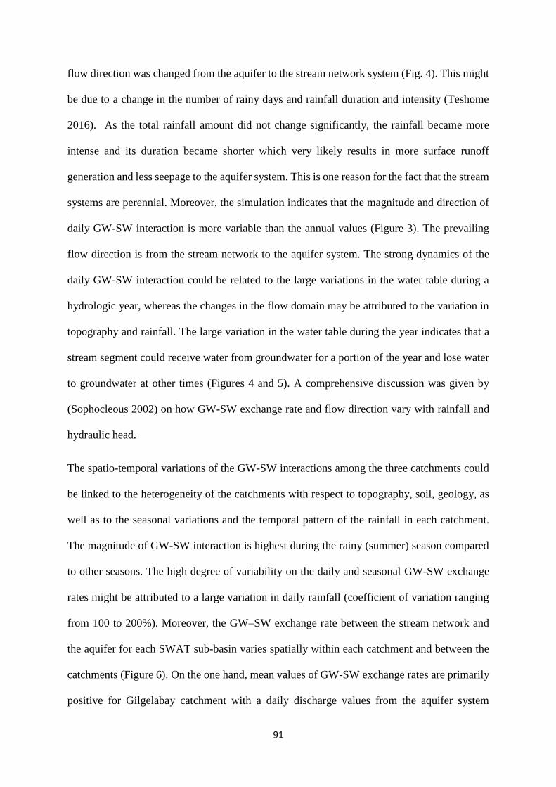
91
flow direction was changed from the aquifer to the stream network system (Fig. 4). This might
be due to a change in the number of rainy days and rainfall duration and intensity (Teshome
2016). As the total rainfall amount did not change significantly, the rainfall became more
intense and its duration became shorter which very likely results in more surface runoff
generation and less seepage to the aquifer system. This is one reason for the fact that the stream
systems are perennial. Moreover, the simulation indicates that the magnitude and direction of
daily GW-SW interaction is more variable than the annual values (Figure 3). The prevailing
flow direction is from the stream network to the aquifer system. The strong dynamics of the
daily GW-SW interaction could be related to the large variations in the water table during a
hydrologic year, whereas the changes in the flow domain may be attributed to the variation in
topography and rainfall. The large variation in the water table during the year indicates that a
stream segment could receive water from groundwater for a portion of the year and lose water
to groundwater at other times (Figures 4 and 5). A comprehensive discussion was given by
(Sophocleous 2002) on how GW-SW exchange rate and flow direction vary with rainfall and
hydraulic head.
The spatio-temporal variations of the GW-SW interactions among the three catchments could
be linked to the heterogeneity of the catchments with respect to topography, soil, geology, as
well as to the seasonal variations and the temporal pattern of the rainfall in each catchment.
The magnitude of GW-SW interaction is highest during the rainy (summer) season compared
to other seasons. The high degree of variability on the daily and seasonal GW-SW exchange
rates might be attributed to a large variation in daily rainfall (coefficient of variation ranging
from 100 to 200%). Moreover, the GW–SW exchange rate between the stream network and
the aquifer for each SWAT sub-basin varies spatially within each catchment and between the
catchments (Figure 6). On the one hand, mean values of GW-SW exchange rates are primarily
positive for Gilgelabay catchment with a daily discharge values from the aquifer system
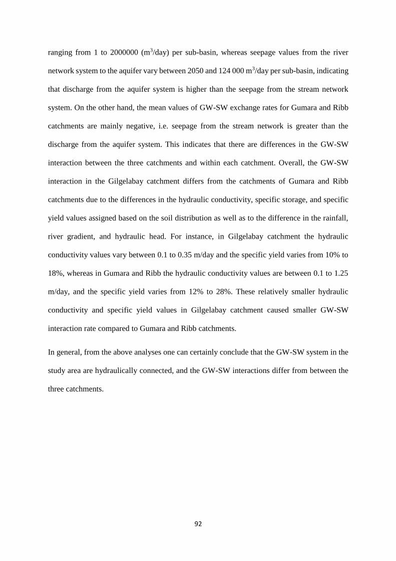
92
ranging from 1 to 2000000 (m3/day) per sub-basin, whereas seepage values from the river
network system to the aquifer vary between 2050 and 124 000 m3/day per sub-basin, indicating
that discharge from the aquifer system is higher than the seepage from the stream network
system. On the other hand, the mean values of GW-SW exchange rates for Gumara and Ribb
catchments are mainly negative, i.e. seepage from the stream network is greater than the
discharge from the aquifer system. This indicates that there are differences in the GW-SW
interaction between the three catchments and within each catchment. Overall, the GW-SW
interaction in the Gilgelabay catchment differs from the catchments of Gumara and Ribb
catchments due to the differences in the hydraulic conductivity, specific storage, and specific
yield values assigned based on the soil distribution as well as to the difference in the rainfall,
river gradient, and hydraulic head. For instance, in Gilgelabay catchment the hydraulic
conductivity values vary between 0.1 to 0.35 m/day and the specific yield varies from 10% to
18%, whereas in Gumara and Ribb the hydraulic conductivity values are between 0.1 to 1.25
m/day, and the specific yield varies from 12% to 28%. These relatively smaller hydraulic
conductivity and specific yield values in Gilgelabay catchment caused smaller GW-SW
interaction rate compared to Gumara and Ribb catchments.
In general, from the above analyses one can certainly conclude that the GW-SW system in the
study area are hydraulically connected, and the GW-SW interactions differ from between the
three catchments.
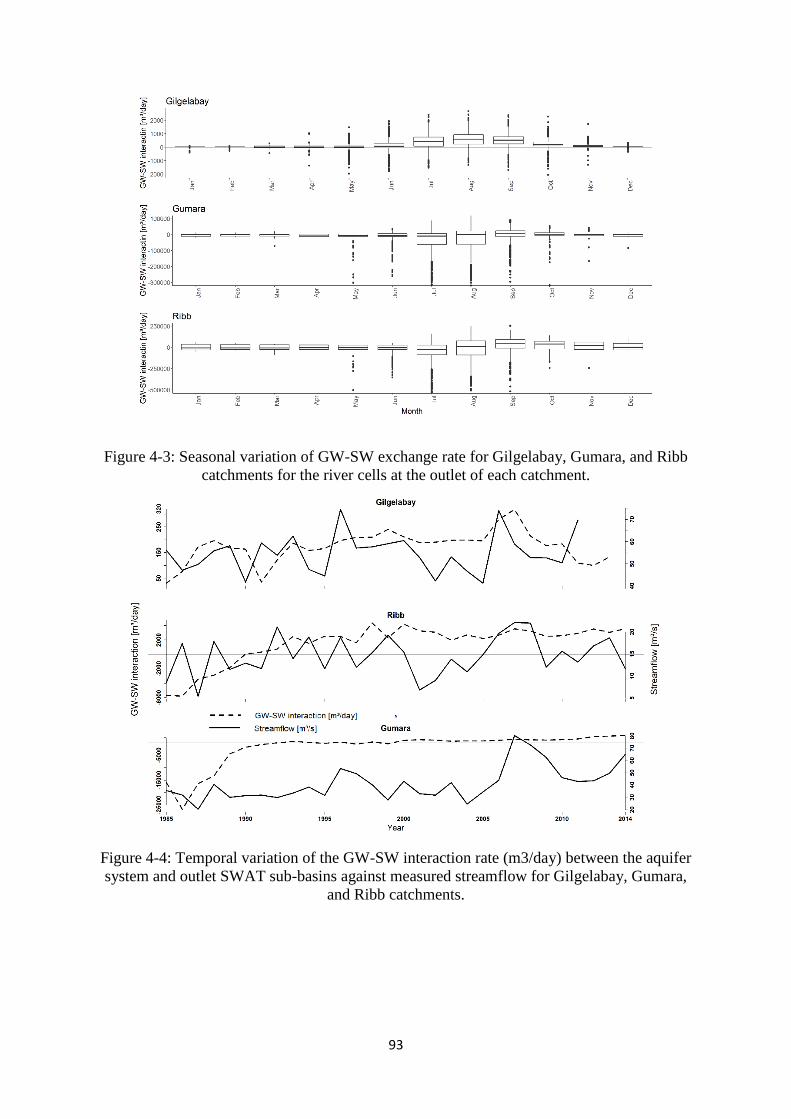
93
Figure 4-3: Seasonal variation of GW-SW exchange rate for Gilgelabay, Gumara, and Ribb
catchments for the river cells at the outlet of each catchment.
Figure 4-4: Temporal variation of the GW-SW interaction rate (m3/day) between the aquifer
system and outlet SWAT sub-basins against measured streamflow for Gilgelabay, Gumara,
and Ribb catchments.
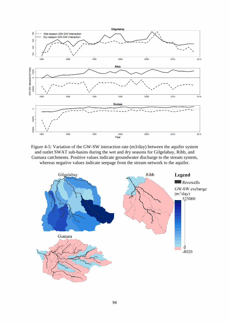
94
Figure 4-5: Variation of the GW-SW interaction rate (m3/day) between the aquifer system
and outlet SWAT sub-basins during the wet and dry seasons for Gilgelabay, Ribb, and
Gumara catchments. Positive values indicate groundwater discharge to the stream system,
whereas negative values indicate seepage from the stream network to the aquifer.
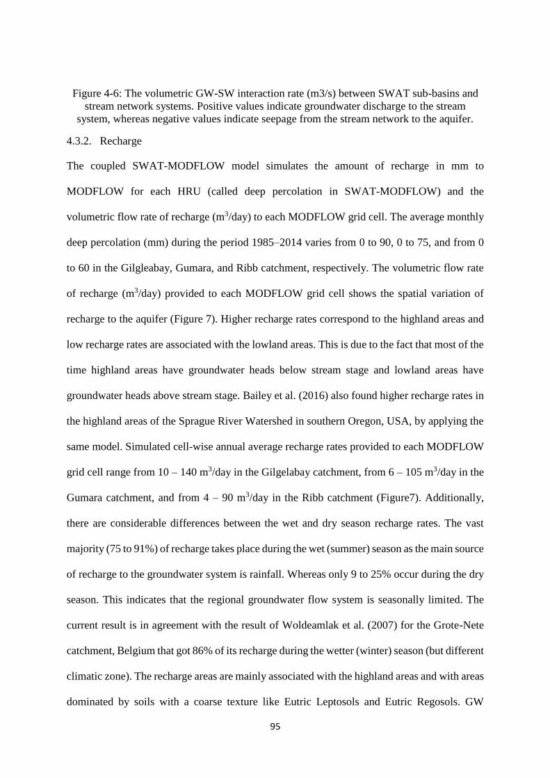
95
Figure 4-6: The volumetric GW-SW interaction rate (m3/s) between SWAT sub-basins and
stream network systems. Positive values indicate groundwater discharge to the stream
system, whereas negative values indicate seepage from the stream network to the aquifer.
4.3.2. Recharge
The coupled SWAT-MODFLOW model simulates the amount of recharge in mm to
MODFLOW for each HRU (called deep percolation in SWAT-MODFLOW) and the
volumetric flow rate of recharge (m3/day) to each MODFLOW grid cell. The average monthly
deep percolation (mm) during the period 1985–2014 varies from 0 to 90, 0 to 75, and from 0
to 60 in the Gilgleabay, Gumara, and Ribb catchment, respectively. The volumetric flow rate
of recharge (m3/day) provided to each MODFLOW grid cell shows the spatial variation of
recharge to the aquifer (Figure 7). Higher recharge rates correspond to the highland areas and
low recharge rates are associated with the lowland areas. This is due to the fact that most of the
time highland areas have groundwater heads below stream stage and lowland areas have
groundwater heads above stream stage. Bailey et al. (2016) also found higher recharge rates in
the highland areas of the Sprague River Watershed in southern Oregon, USA, by applying the
same model. Simulated cell-wise annual average recharge rates provided to each MODFLOW
grid cell range from 10 – 140 m3/day in the Gilgelabay catchment, from 6 – 105 m3/day in the
Gumara catchment, and from 4 – 90 m3/day in the Ribb catchment (Figure7). Additionally,
there are considerable differences between the wet and dry season recharge rates. The vast
majority (75 to 91%) of recharge takes place during the wet (summer) season as the main source
of recharge to the groundwater system is rainfall. Whereas only 9 to 25% occur during the dry
season. This indicates that the regional groundwater flow system is seasonally limited. The
current result is in agreement with the result of Woldeamlak et al. (2007) for the Grote-Nete
catchment, Belgium that got 86% of its recharge during the wetter (winter) season (but different
climatic zone). The recharge areas are mainly associated with the highland areas and with areas
dominated by soils with a coarse texture like Eutric Leptosols and Eutric Regosols. GW
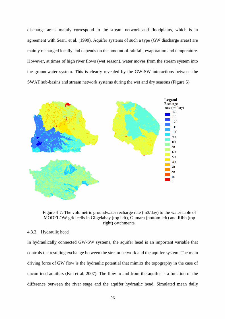
96
discharge areas mainly correspond to the stream network and floodplains, which is in
agreement with Sear1 et al. (1999). Aquifer systems of such a type (GW discharge areas) are
mainly recharged locally and depends on the amount of rainfall, evaporation and temperature.
However, at times of high river flows (wet season), water moves from the stream system into
the groundwater system. This is clearly revealed by the GW-SW interactions between the
SWAT sub-basins and stream network systems during the wet and dry seasons (Figure 5).
Figure 4-7: The volumetric groundwater recharge rate (m3/day) to the water table of
MODFLOW grid cells in Gilgelabay (top left), Gumara (bottom left) and Ribb (top
right) catchments.
4.3.3. Hydraulic head
In hydraulically connected GW-SW systems, the aquifer head is an important variable that
controls the resulting exchange between the stream network and the aquifer system. The main
driving force of GW flow is the hydraulic potential that mimics the topography in the case of
unconfined aquifers (Fan et al. 2007). The flow to and from the aquifer is a function of the
difference between the river stage and the aquifer hydraulic head. Simulated mean daily
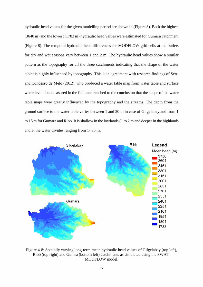
97
hydraulic head values for the given modelling period are shown in (Figure 8). Both the highest
(3640 m) and the lowest (1783 m) hydraulic head values were estimated for Gumara catchment
(Figure 8). The temporal hydraulic head differences for MODFLOW grid cells at the outlets
for dry and wet seasons vary between 1 and 2 m. The hydraulic head values show a similar
pattern as the topography for all the three catchments indicating that the shape of the water
tablet is highly influenced by topography. This is in agreement with research findings of Sena
and Condesso de Melo (2012), who produced a water table map from water table and surface
water level data measured in the field and reached to the conclusion that the shape of the water
table maps were greatly influenced by the topography and the streams. The depth from the
ground surface to the water table varies between 1 and 30 m in case of Gilgelabay and from 1
to 15 m for Gumara and Ribb. It is shallow in the lowlands (1 to 2 m and deeper in the highlands
and at the water divides ranging from 1- 30 m.
Figure 4-8: Spatially varying long-term mean hydraulic head values of Gilgelabay (top left),
Ribb (top right) and Gumra (bottom left) catchments as simulated using the SWAT-
MODFLOW model.
98
4.3.4. Implications for water resources management
As the Lake Tana basin is considered as one of the development corridor sites by the
Government of Ethiopia, understanding GW-SW water interaction and implementing
combined use of GW and SW is the top priority for water managers to contribute to a
sustainable development in the region. The present study focuses on the investigation of GW-
SW interaction of three catchments in the Lake Tana basin. Our findings provide insights for
water managers and policy makers for future planning. We found that GW and SW are
hydraulically connected and the stream network systems are dominated by GW flow in
Gilgelabay catchment and vice-versa in Gumara and Ribb catchments. Thus, sustainable water
resources management will be achieved if the future water resource development plan puts a
particular focus on the combined use of groundwater and surface water. The hydraulic head
and GW-SW interaction showed considerable spatial and seasonal variations in all the three
catchments. In Gumara and Ribb catchments, the wet season flow pattern is dominantly from
the river to the aquifer system, whereas the dry season flow is to the river system. This implies
that GW and SW withdrawal e.g. for drinking water use affect this interaction differently in the
wet and dry season. Spatial patterns of the hydraulic head should be considered to define GW
recharge and discharge zones prior to water withdrawal from the aquifer system. Moreover,
understanding the GW-SW interaction is important to characterize the general ecosystem status
as the streamflow in all the three catchments are connected to the GW. Hence GW is critical
with regard to water availability as well as with regard to the control of environmental flow.
4.4. Summary and conclusions
The aim of this study was to investigate GW-SW flow dynamics in the Lake Tana basin by
considering three catchments as case studies (Gilgelabay, Gumara and Ribb) using the coupled
SWAT-MODFLOW model. Results from this study indicated that SWAT-MODFLOW can
simulate the surface and subsurface hydrologic processes in the study areas and can provide
99
insights into GW-SW interactions. The capability of the model to produce reliable results was
reflected by the good match of the simulated and observed streamflow data as well as by the
comparison between observed hydraulic head values measured at water wells during the course
of drilling and mean simulated hydraulic head values. The key findings of this study are:
1. The aquifer and the stream network systems are hydraulically connected in all
catchments in both wet and dry seasons. This was proven by the simulated volumetric
GW-SW exchange rates between each SWAT sub-basin (aquifer) and stream network,
and the stream network and the aquifer for each MODFLOW river cell. The majority
of the flow is from the aquifer to the stream network system particularly in Gilgelabay
catchment.
2. In all catchments, the groundwater and surface water flow system is more variable on
the daily time scale than on the monthly time scale. This was shown by the simulated
results of GW-SW exchange rates, water recharge to the groundwater table and
discharge from the aquifer system.
3. Despite the fact that daily GW-SW exchange rates are highly variable in the Gilgleabay
catchment, the annual volumetric exchange is from the aquifer system to the stream
network system indicating that stream systems are gaining.
4. In both Gumara and Ribb catchments, the annual volumetric GW-SW exchange rates
are more dynamic in time compared to Gilgelabay catchment. This was suggested by
the GW-SW exchange rates between each SWAT sub-basin and stream network
systems (Fig. 5 and 6). During the wet seasons, the flows dominantly from the stream
system to the aquifer, while it is from the aquifer to the stream network system during
the dry season.
5. The annual GW-SW exchange rates at the outlet sub-basins show a change in the flow
direction of water for Gumara and Ribb after 1995 and 1991, respectively (Fig. 4).
100
Before the mentioned years, the flow system was from the stream network to the aquifer
system and after these years the flow direction changed from the aquifer system to the
stream network. This might be related to the decline with the number of rainy days
(specially the dry season) since 1990 while the total annual rainfall was not significantly
changed.
6. The modelling results have been checked for their reliability using measured and
simulated streamflow time series and hydraulic head values measured during the
drilling of wells. However, the model could be improved if regularly measured time
series of water table elevation and stream stage values were available.
7. This study primarily focuses on the setup of a coupled SW and GW model to understand
the hydrodynamic condition of the GW-SW system in the study area. The model is
valuable because it can be used to assess climate change impacts on groundwater
resources in the future.
101
5. Climate change impacts on the water and groundwater resources of the
Lake Tana Basin, Ethiopia
*Tibebe B. Tigabu1, Paul D. Wagner1, Georg Hörmann1, Jens Kiesel1,2 and
Nicola Fohrer1
1 Department of Hydrology and Water Resources Management, Institute for Natural Resource
Conservation, Kiel University, D-24118 Kiel, Germany
2 Leibniz-Institute of Freshwater Ecology and Inland Fisheries (IGB), Department of Ecosystem
Research, Müggelseedamm 301, 12587 Berlin, Germany
Address of corresponding author: Tibebe Tigabu, Department of Hydrology and Water
Resources Management, Institute of Natural Resource Conservation, CAU, D-24118 Kiel,,
Germany, E-mail: [email protected]
To be submitted until 20th April 2020
102
Abstract
Climate change causes strong impacts on water resources. In particular, the mid- to long-
term effect on groundwater will be challenging in many regions, which rely on
groundwater to meet their water demands. This is the case in the Lake Tana basin,
Ethiopia, where discharge regimes are dominated by base flow from the shallow aquifer.
The Lake Tana basin has more than three million inhabitants and the required water is
largely extracted from groundwater. Therefore, the potential impact of climate change on
the major water balance components has been assessed in the Lake Tana basin for two
future periods: mid-term (2031-2060) and long-term (2065-2094) assuming that
anticipated changes of temperature and rainfall would cause substantial impact on major
hydrological components. We focus on changes in the groundwater contribution to
stream flow (GWQ) and other major water balance components (actual
evapotranspiration, surface runoff, and water yield) in two tributary catchments (Gumara
and Gilgelabay) of the Lake Tana basin. The hydrologic model SWAT was used to assess
likely changes under two representative concentration pathways (RCP4.5 and 8.5). Under
the utilized RCPs, average temperature is expected to increase by 2.2°C and 3.6°C for
the mid-term and long-term of the century, respectively. We used a total of 35 bias
corrected regional climate models (RCMs) from the CORDEX dataset for both
catchments. Compared to the baseline average, outcomes of this research revealed that
the groundwater contribution to stream flow is projected to decrease whereas surface
runoff is projected to increase. No or only slight changes in rainfall are expected, but the
number of days with rainfall is expected to decrease in both catchments under the two
concentration pathways. In conclusion, these results could have considerable advantages
for the future water resource management and planning in the basin and other similar
regions expecting significance warming.

103
Keywords: Climate change, groundwater, water balance, surface runoff, SWAT, Ethiopia.
104
5.1. Introduction
Climate change causes strong impacts on the natural systems on all continents (Field et al.
2014). The water cycle is highly affected by climate change. There are many evidences that
show impact of climate change on different components of the hydrologic cycle across the
globe. According to (Marx et al. 2018), half of the rivers in Europe will experience decreases
in the low flow (7% - 12%) under 1.5 K warming for the period 2047-2076. A review paper by
Meixner et al. (2016) in US reported likely declines in the recharge of aquifers in the western
US during the end of the 21st century. Under RCP4.5, Ndhlovu and Woyessa (2020) found a
slight decrease (1%) in the annual rainfall, whereas water yield and runoff will increase by 5%
and 6%, respectively for the period of 2020–2050 in the Zambezi River Basin, Africa.
Gebremeskel and Kebedeb (2018) reported 13% and 14% declines of surface runoff under A1B
and B1 scenarios, respectively for the period 2015-2050 in Werii watershed of the Tekeze
River, Ethiopia. The annual mean soil moisture is also anticipated to decrease in most
subtropical regions (IPCC 2014). Consequently, uncertainties associated with future water
resources management are growing due to the effect of climate change (Abbaspour et al. 2015).
To minimize uncertainties associated with future water management plans and to secure the
future water needs of the global community, many efforts have been made in investigating the
impact of climate change on water resources across the planet. However, the majority of the
studies focuses more on surface water bodies than on groundwater (Meixner et al. 2016; Saha
et al. 2017), and African countries are underrepresented in these efforts (Field et al. 2014). It is
well known that the social-ecological systems of developing countries are severely impacted
by climate change due to the lowest capacity to adapt (Dille et al. 2018). This indicates that
more efforts are required to investigate the effect of climate change in developing countries
like Ethiopia.
105
Compared to surface water, groundwater is a reliable and cost-effective resource especially
in many African countries and other parts of the world where availability of surface water
is limited (Bovolo et al. 2009). One third of the global freshwater is extracted from the
groundwater source (Taylor et al. 2013). In Ethiopia, groundwater provides 80% of the
national water demand (Kebede 2018). This national condition is the same in the Lake Tana
basin.
In the Lake Tana basin, being a home for more than three million people and a head water
source of the Blue Nile River, several studies were carried out to investigate the impact of
climate change on its hydrology. Nevertheless, the vast majority of the climate change
studies were focused on streamflow or runoff analyses and there are disagreements in their
findings (Abdo et al. 2009; Taye et al. 2011; Dile et al. 2013). Adbo et al. (2009) and Dile
et al. (2013) studied the hydrologic responses of Gilgelabay catchment under climate
change. According to Dile et al. (2013), the monthly mean volume of runoff in Gilgelabay
catchment tends to increase significantly (up to 135%) for the mid and long-term of the
21st century. Contrary to Dile et al. (2013), Abdo et al. (2009) reported decreases in the
monthly mean runoff in the same catchment. Taye et al. (2011) also studied the future
development of streamflow in the Lake Tana basin under climate change. In this study,
both increases and decreases (-75% to 81%) of streamflow are expected during 2050s in
different catchments in Upper Blue Nile Basin. Groundwater contributes a substantial
amount of water to the flow of streams in the Lake Tana basin. Even though it has a
significant contribution to the streamflow (Setegn et al. 2008; Tigabu et al. 2019), all past
studies ignored it in their analyses. The only studies that addressed multiple water balance
components and groundwater flow analyses under climate change in the Lake Tana basin
are Setegn et al. (2011) and Woldesenbet et al. (2018). Setegn et al. (2011) analysed the
responses of streamflow, actual evapotranspiration, soil moisture, and groundwater
106
contribution to the streamflow based on 17 GCM outputs from the World Climate Research
Programme’s Coupled Model Intercomparison Project phase 3 (CMIP3). Their results
indicated that the annual streamflow tends to decline significantly for most of the GCMs
considered for the study, while the actual evapotranspiration is expected to increase. A
likely decrease of groundwater flow and soil moisture was reported. However, the
magnitudes of changes in the groundwater flow as well as the spatial patterns of changes
were not considered. Woldesenbet et al. (2018) also studied the impacts of future climate
change on the hydrological components of the Lake Tana Basin under RCP6.0. Their
results showed that the groundwater contribution to the streamflow, percolation, and actual
evapotranspiration would increase on the annual time scale, but decreases are expected
during the small rainy season compared to their reference period (1980-2005). Although
this research is comprehensive in addressing the major water balance components, it does
not address the impact of climate change on the major hydrological components during the
mid-term and long-term of the 21st century as the authors focused only on a short-term
period (2016–2030). In addition, high level concentration pathways were not considered.
Thus, the main purpose of this study is to enhance our understanding of how projected
changes in rainfall and temperature will affect the groundwater contribution to the
streamflow and other major water balance components in Gilgelabay and Gumara
catchments, which are the two major tributaries of Lake Tana during the mid-term (2031-
2060) and long-term (2065-2094). The specific objectives are i) to assess if groundwater
contribution to the streamflow and other major water balance components have
significantly changed in response to climate change and ii) to determine if changes in the
groundwater contribution to the streamflow show a distinct spatial pattern in the study area.
107
5.2. Materials and methods
5.2.1. Study area
The Lake Tana basin is entirely located in the Amhara regional state in the north-western
highlands of Ethiopia (Figure 1). It is one of the sub-basins of the Blue Nile River in which the
largest fresh water lake in the country is found. The total catchment area of the Lake Tana basin
is 15,321 km2. More than 40 streams are flowing into Lake Tana (Alemayehu et al. 2010).
Among others, Gilgelabay and Gumara contribute about 70% of the inflow to the lake. The
Blue Nile (locally referred to as Abay) is the only surface outflow from the lake with an average
annual flow volume, as calculated from raw data (1973 to 2014), of 3.9 billion m3 (123 m3/s)
measured at the lake outlet.
Similar to its hydrologic variability, the Lake Tana basin has a heterogeneous hydrogeology.
According to Kebede et al. (2005), areas surrounding Lake Tana are covered by quaternary
basalts and alluvial sediments. These geologic formations are characterized by high
groundwater transmissivity that vary 100–700 m2/day. The highland part of the basin on the
other hand is covered by the basaltic plateau, where the groundwater transmissivity is lower
compared to the quaternary basalt and sediments (Kebede et al. 2005). Being driven by the
diversified parent geology, the soil structure, lateral and vertical extents, and hydraulic
conductivity the basin is highly diversified. The soils vary from hydrologic group B to group
D, which represent infiltration rates from moderate to very slow. Additional information can
be found in Tigabu et al. (2019). Gilgelabay and Gumara are the two perennial rivers that are
characterised by a succession between bedrock types in their higher reaches, and alluvial types
in their lower reaches and floodplains (Poppe et al. 2013). There is a significant topographic
variation between the lowland and the mountain ranges. This diversified topographic feature
of the catchment and the movement of the inter-tropical convergence zone (ITCZ) result in a
spatially varying rainfall pattern in the basin. June to September is the rainy season in the
108
catchment corresponding to the ITCZ position north of the Equator. The amount of annual
rainfall is directly related to elevation above mean sea level: high rainfall is observed in the
highlands, whereas low rainfall is measured in the lowlands (Tigabu et al. 2018). Moreover,
large (global) atmospheric circulation and sea surface temperatures such as large scale forcing
through El Niño Southern Oscillation (ENSO), Quasi-Biennial Oscillation (QBO), as well as
west-east sea surface temperature gradients over the equatorial Indian Ocean are significantly
influencing rainfall variability (Omondi et al. 2014). The catchments are characterized by
intensive agriculture. About 60% of catchments are cultivated land.
5.2.2. Data base
Daily rainfall and minimum and maximum temperature values from 5 meteorological stations
for the years 1980 to 2014 were used, which were provided by the National Meteorological
Service Agency (NMA 2016). Daily streamflow data of Gilgelabay near Merawi, and Gumara
near Bahirdar gauging stations for the years 1980 to 2014 were obtained from the Department
of Hydrology, Ministry of Water, Irrigation and Electricity of the Ethiopian Government
(MoWIE 2016).
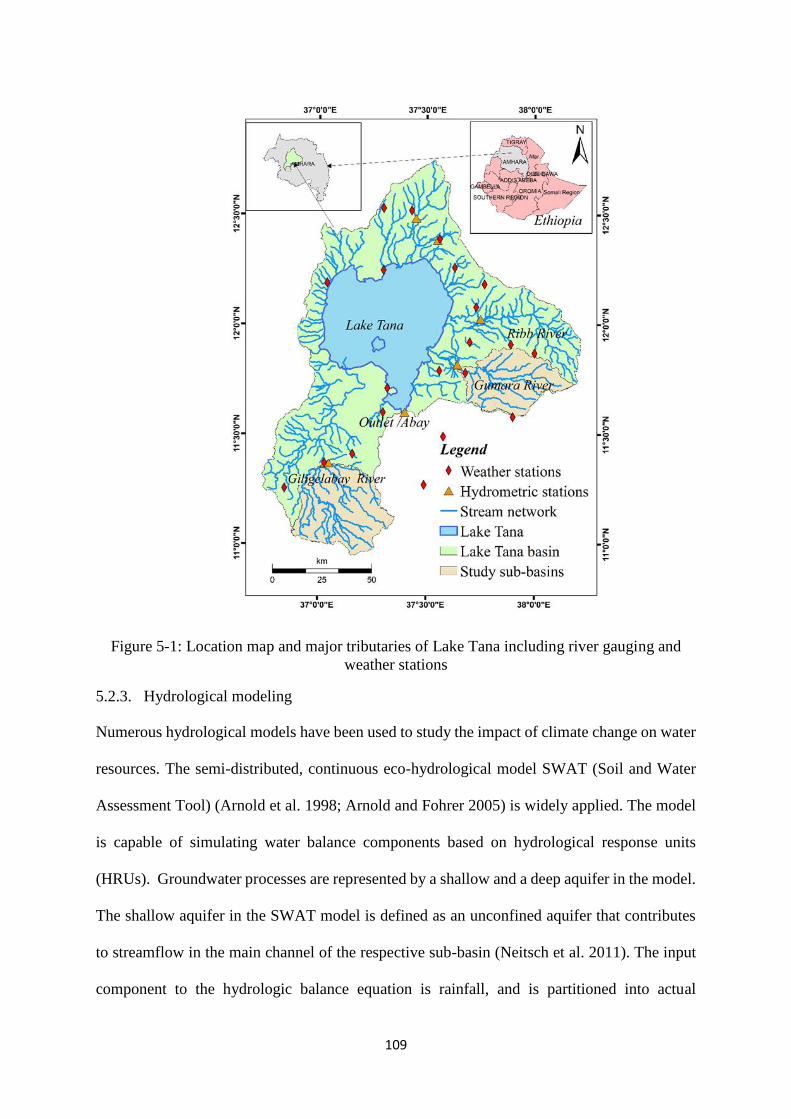
109
Figure 5-1: Location map and major tributaries of Lake Tana including river gauging and
weather stations
5.2.3. Hydrological modeling
Numerous hydrological models have been used to study the impact of climate change on water
resources. The semi-distributed, continuous eco-hydrological model SWAT (Soil and Water
Assessment Tool) (Arnold et al. 1998; Arnold and Fohrer 2005) is widely applied. The model
is capable of simulating water balance components based on hydrological response units
(HRUs). Groundwater processes are represented by a shallow and a deep aquifer in the model.
The shallow aquifer in the SWAT model is defined as an unconfined aquifer that contributes
to streamflow in the main channel of the respective sub-basin (Neitsch et al. 2011). The input
component to the hydrologic balance equation is rainfall, and is partitioned into actual
110
evapotranspiration, water entering to the vadose zone, and surface runoff.
In this study, calibrated SWAT models for Gilgelabay and Gumara catchments (Tigabu et al.
2019) were used. The model showed a reasonable performance on the daily time scale (NSE>
0.65, KGE>0.62, R2>0.8, RSR<0.5, and PBIAS <21%, validation period, Moriasi et al. 2007.
In addition to statistical indices, the fitness of the models in capturing the monthly streamflow
data were also evaluated by comparing the measured and simulated streamflow hydrographs
and flow duration curves. The simulated hydrographs and flow duration curves were
consistence with the measured ones indicating that the models are capable of simulating
hydrologic processes in study catchments. The flow duration curves showed very good
agreement for the middle and low flow conditions in both catchments, which are indicative of
representing groundwater contribution to streamflow. Hence the model is suitable for assessing
the impacts of climate change on groundwater and water resources in the two catchments.
Detailed information on the parameters and calibration procedures are available in Tigabu et
al. (2019). As the magnitude of groundwater flow in a catchment is counterbalanced by the
other hydrologic components, we also analysed ET, SURQ, soil moisture content, and
percolation.
5.2.4. Projected climate change data
To assess impacts of future climate change on water resources different emission scenarios as
expressed in the representative concentration pathways (RCPs) are used. Global Circulation
Models (GCMs) and the Coordinated Regional climate Downscaling Experiment (CORDEX)
are the most commonly applied and physically based ways in formulating different climate
scenarios (Elshamy et al. 2009). Nevertheless, GCMs are unsuitable for local climate impact
studies due to their coarse spatial resolution and incapability to capture local effects (Navarro-
Racines et al. 2020). To overcome these limitations, regional climate models (RCMs) are
applied to downscale GCM outputs (Eden et al. 2014; Mascaro et al. 2015). CORDEX
111
coordinates RCMs to improve regional climate downscaling models and techniques and to
produce coordinated sets of regional downscaled projections worldwide (Giorgi and Gutowski
Jr 2015). There are multiple CORDEX domains worldwide including the CORDEX African
domain. Although RCM outputs provide a better spatial and temporal resolution than GCM
outputs, projected temperature and rainfall are still biased (Berg et al. 2012). Consequently, a
number of bias correction methods are available to overcome this problem. The main
adjustment methods are based on the mean, both mean and variance, and quantile values.
Among others, linear scaling and local intensity scaling, power transformation method,
distribution mapping or quantile mapping are widely applied (Smitha et al. 2018).
Climate models can project future rainfall and temperature. However, there are considerable
differences and uncertainties in the projected rainfall among the different climate models
(Kling et al. 2012; Kiesel et al. 2019). According to Mascaro et al. (2015), the CORDEX-
African RCMs have significant biases among the individual models. For this reason, an
ensemble modeling approach that depends on a number of RCMs is required to minimize biases
and obtain a representative result (Kling et al. 2012).
Past climate change studies in the Lake Tana basin were mainly based on single GCM (Abdo
et al. 2009; Dile et al. 2013; Adem et al. 2016) at the Coupled Model Intercomparison Project
(CMIP3) results. However, model outputs from CMIP3 have course spatial resolutions and are
not as comprehensive as model outputs from CMIP5 (Taylor et al. 2012). According to Taylor
et al. (2012) and Stocker et al. (2013), climate models under CMIP5 are capable to represent
bio-geological processes, aerosols and carbon cycles that interact with physical climate. As a
result, better simulations are expected under CMIP5 than under CMIP3. Reports by Maher et
al. (2017) and Kusunoki and Arakawa (2015) indicated that annual and seasonal rainfall
simulated from CMIP5 showed higher reproducibility than CMIP3 over the western Himalayan
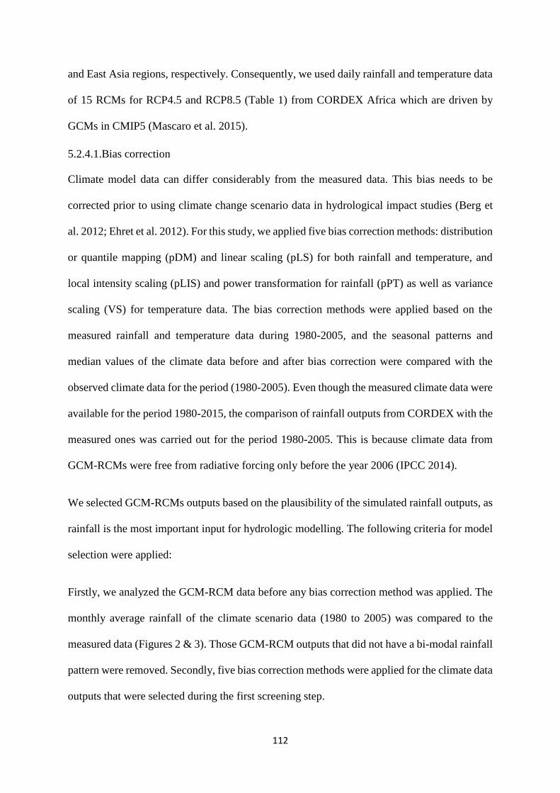
112
and East Asia regions, respectively. Consequently, we used daily rainfall and temperature data
of 15 RCMs for RCP4.5 and RCP8.5 (Table 1) from CORDEX Africa which are driven by
GCMs in CMIP5 (Mascaro et al. 2015).
5.2.4.1.Bias correction
Climate model data can differ considerably from the measured data. This bias needs to be
corrected prior to using climate change scenario data in hydrological impact studies (Berg et
al. 2012; Ehret et al. 2012). For this study, we applied five bias correction methods: distribution
or quantile mapping (pDM) and linear scaling (pLS) for both rainfall and temperature, and
local intensity scaling (pLIS) and power transformation for rainfall (pPT) as well as variance
scaling (VS) for temperature data. The bias correction methods were applied based on the
measured rainfall and temperature data during 1980-2005, and the seasonal patterns and
median values of the climate data before and after bias correction were compared with the
observed climate data for the period (1980-2005). Even though the measured climate data were
available for the period 1980-2015, the comparison of rainfall outputs from CORDEX with the
measured ones was carried out for the period 1980-2005. This is because climate data from
GCM-RCMs were free from radiative forcing only before the year 2006 (IPCC 2014).
We selected GCM-RCMs outputs based on the plausibility of the simulated rainfall outputs, as
rainfall is the most important input for hydrologic modelling. The following criteria for model
selection were applied:
Firstly, we analyzed the GCM-RCM data before any bias correction method was applied. The
monthly average rainfall of the climate scenario data (1980 to 2005) was compared to the
measured data (Figures 2 & 3). Those GCM-RCM outputs that did not have a bi-modal rainfall
pattern were removed. Secondly, five bias correction methods were applied for the climate data
outputs that were selected during the first screening step.
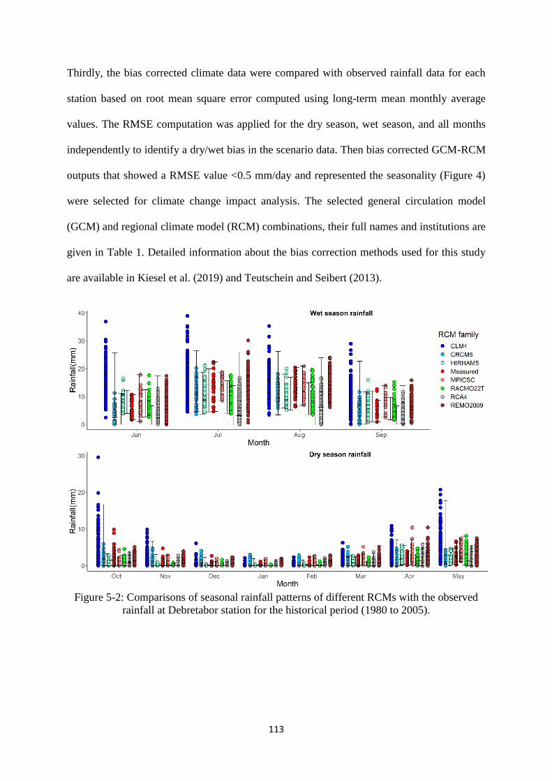
113
Thirdly, the bias corrected climate data were compared with observed rainfall data for each
station based on root mean square error computed using long-term mean monthly average
values. The RMSE computation was applied for the dry season, wet season, and all months
independently to identify a dry/wet bias in the scenario data. Then bias corrected GCM-RCM
outputs that showed a RMSE value <0.5 mm/day and represented the seasonality (Figure 4)
were selected for climate change impact analysis. The selected general circulation model
(GCM) and regional climate model (RCM) combinations, their full names and institutions are
given in Table 1. Detailed information about the bias correction methods used for this study
are available in Kiesel et al. (2019) and Teutschein and Seibert (2013).
Figure 5-2: Comparisons of seasonal rainfall patterns of different RCMs with the observed
rainfall at Debretabor station for the historical period (1980 to 2005).
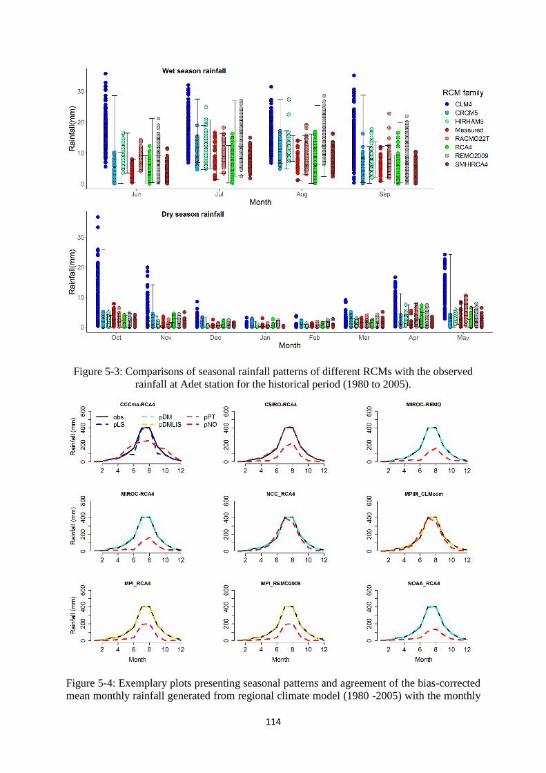
114
Figure 5-3: Comparisons of seasonal rainfall patterns of different RCMs with the observed
rainfall at Adet station for the historical period (1980 to 2005).
Figure 5-4: Exemplary plots presenting seasonal patterns and agreement of the bias-corrected
mean monthly rainfall generated from regional climate model (1980 -2005) with the monthly
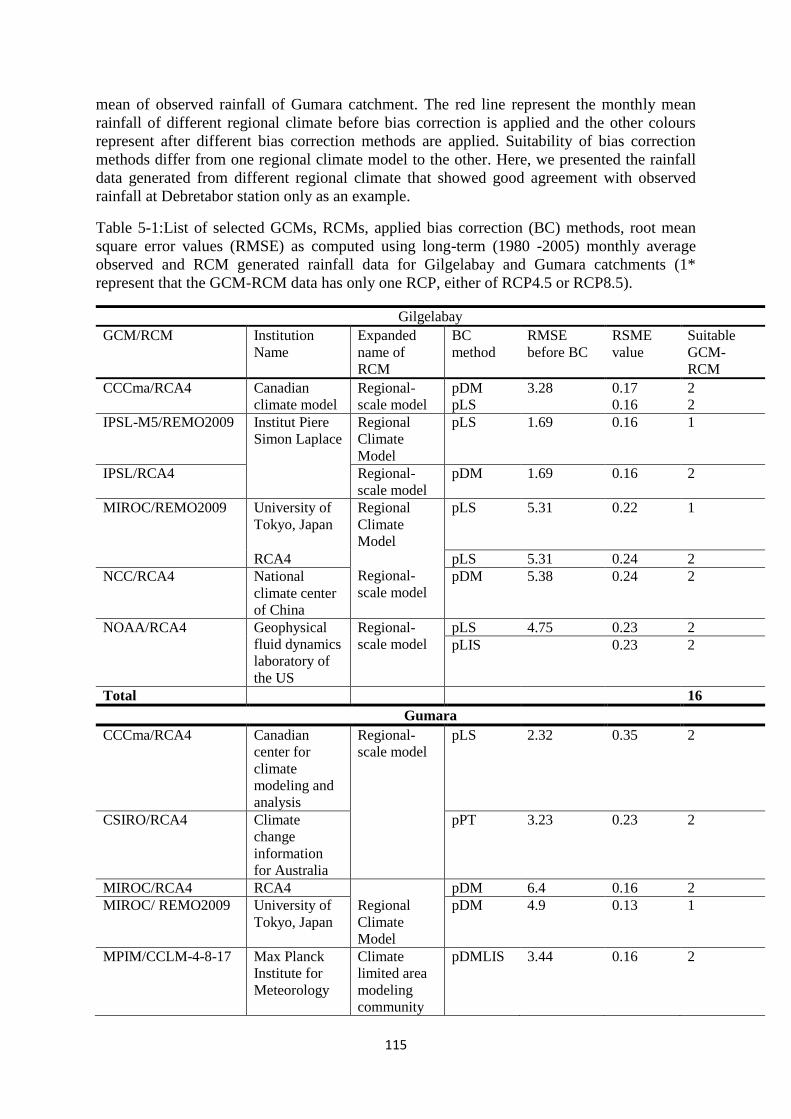
115
mean of observed rainfall of Gumara catchment. The red line represent the monthly mean
rainfall of different regional climate before bias correction is applied and the other colours
represent after different bias correction methods are applied. Suitability of bias correction
methods differ from one regional climate model to the other. Here, we presented the rainfall
data generated from different regional climate that showed good agreement with observed
rainfall at Debretabor station only as an example.
Table 5-1:List of selected GCMs, RCMs, applied bias correction (BC) methods, root mean
square error values (RMSE) as computed using long-term (1980 -2005) monthly average
observed and RCM generated rainfall data for Gilgelabay and Gumara catchments (1*
represent that the GCM-RCM data has only one RCP, either of RCP4.5 or RCP8.5).
Gilgelabay
GCM/RCM Institution
Name
Expanded
name of
RCM
BC
method
RMSE
before BC
RSME
value
Suitable
GCM-
RCM
CCCma/RCA4 Canadian
climate model
Regional-
scale model
pDM 3.28 0.17 2
pLS 0.16 2
IPSL-M5/REMO2009 Institut Piere
Simon Laplace
Regional
Climate
Model
pLS 1.69 0.16 1
IPSL/RCA4 Regional-
scale model
pDM 1.69 0.16 2
MIROC/REMO2009 University of
Tokyo, Japan
Regional
Climate
Model
pLS 5.31 0.22 1
RCA4
Regional-
scale model
pLS 5.31 0.24 2
NCC/RCA4 National
climate center
of China
pDM 5.38 0.24 2
NOAA/RCA4 Geophysical
fluid dynamics
laboratory of
the US
Regional-
scale model
pLS 4.75 0.23 2
pLIS 0.23 2
Total 16
Gumara
CCCma/RCA4 Canadian
center for
climate
modeling and
analysis
Regional-
scale model
pLS 2.32 0.35 2
CSIRO/RCA4 Climate
change
information
for Australia
pPT 3.23 0.23 2
MIROC/RCA4 RCA4 pDM 6.4 0.16 2
MIROC/ REMO2009 University of
Tokyo, Japan
Regional
Climate
Model
pDM 4.9 0.13 1
MPIM/CCLM-4-8-17 Max Planck
Institute for
Meteorology
Climate
limited area
modeling
community
pDMLIS 3.44 0.16 2
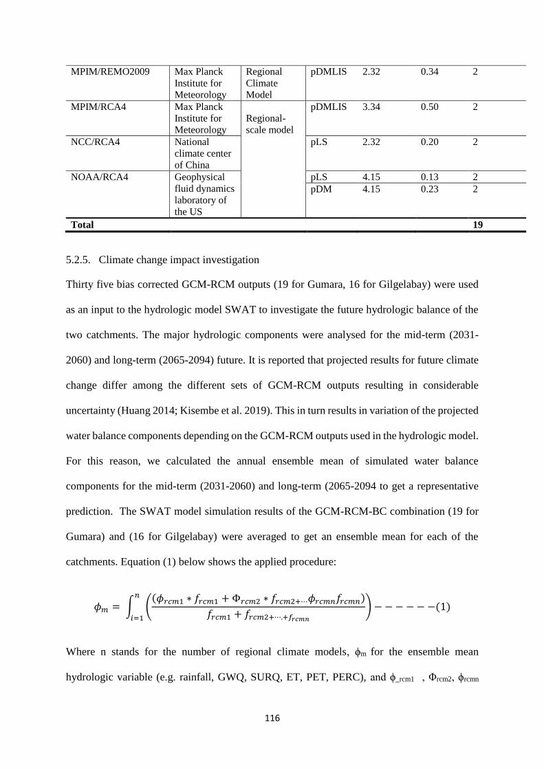
116
MPIM/REMO2009 Max Planck
Institute for
Meteorology
Regional
Climate
Model
pDMLIS 2.32 0.34 2
MPIM/RCA4 Max Planck
Institute for
Meteorology
Regional-
scale model
pDMLIS 3.34 0.50 2
NCC/RCA4 National
climate center
of China
pLS 2.32 0.20 2
NOAA/RCA4 Geophysical
fluid dynamics
laboratory of
the US
pLS 4.15 0.13 2
pDM 4.15 0.23 2
Total 19
5.2.5. Climate change impact investigation
Thirty five bias corrected GCM-RCM outputs (19 for Gumara, 16 for Gilgelabay) were used
as an input to the hydrologic model SWAT to investigate the future hydrologic balance of the
two catchments. The major hydrologic components were analysed for the mid-term (2031-
2060) and long-term (2065-2094) future. It is reported that projected results for future climate
change differ among the different sets of GCM-RCM outputs resulting in considerable
uncertainty (Huang 2014; Kisembe et al. 2019). This in turn results in variation of the projected
water balance components depending on the GCM-RCM outputs used in the hydrologic model.
For this reason, we calculated the annual ensemble mean of simulated water balance
components for the mid-term (2031-2060) and long-term (2065-2094 to get a representative
prediction. The SWAT model simulation results of the GCM-RCM-BC combination (19 for
Gumara) and (16 for Gilgelabay) were averaged to get an ensemble mean for each of the
catchments. Equation (1) below shows the applied procedure:
𝜙𝑚 = ∫ ((𝜙𝑟𝑐𝑚1 ∗ 𝑓𝑟𝑐𝑚1 + Φ𝑟𝑐𝑚2 ∗ 𝑓𝑟𝑐𝑚2+⋯𝜙𝑟𝑐𝑚𝑛𝑓𝑟𝑐𝑚𝑛)
𝑓𝑟𝑐𝑚1 + 𝑓𝑟𝑐𝑚2+⋯.+𝑓𝑟𝑐𝑚𝑛
) − − − − − −(1)𝑛
𝑖=1
Where n stands for the number of regional climate models, ϕm for the ensemble mean
hydrologic variable (e.g. rainfall, GWQ, SURQ, ET, PET, PERC), and ϕ_rcm1 , Φrcm2, ϕrcmn
117
represent the value of hydrologic variable at the given regional climate model1, 2, 3….n and f
represents the frequency of the regional climate model depending on the selected bias
correction method.
The changes of the major water balance components were computed with reference to SWAT
model simulated results using observed climate data (1985-2014) here after called baseline
period. Tukey’s multiple mean comparison test was applied to investigate the projected water
balance changes. Here, factor variables named baseline, mid-term, and long-term were
assigned for each year corresponding to the three time periods. Then a Tukey multiple mean
comparison test (95% confidence level) that is based on a two way anova model (Yandell 1997)
was applied between the baseline and mid-term, baseline and long-term, mid-term and long-
term major water balance components and climate time series.
5.3. Results and discussions
5.3.1. Project changes of Rainfall and Temperature
A combination of 7 GCM, 4 RCM, and 5 BC resulting in a total of 35 GCM-RCM-BC scenario
outputs (19 for Gumara) and (16 for Gilgelabay) were used in SWAT to simulate the effect of
climate change on the hydrologic balances of the two catchments considered. Rainfall
comparison between measured and climate scenario data for the period 1980 to 2005 showed
that there is no single bias correction method that performed best for all RCMs (Table 2). We
observed variation in matching the measured mean monthly rainfall. In the case of CCCma-
RCA4 and NCC-RCA4, all BC correction methods showed miss-matches (RMSE values vary
between 1.53 to 3.34) on the mean monthly rainfall values except the pLS (Table 1) method.
The pLS BC method showed relatively better matching of the mean value for each month than
the other BC methods (RMSE < 0.35). Power transformation for rainfall (pPT) was the best
BC method in fitting the mean rainfall values and maintaining the seasonal patterns in the case
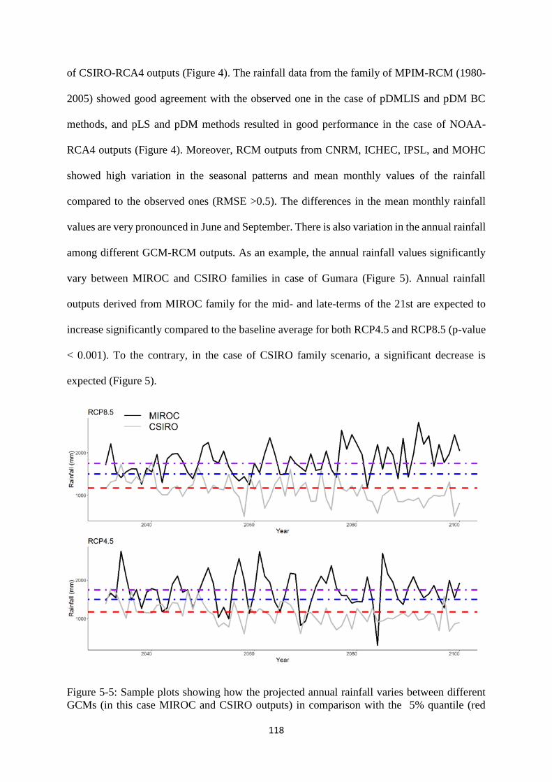
118
of CSIRO-RCA4 outputs (Figure 4). The rainfall data from the family of MPIM-RCM (1980-
2005) showed good agreement with the observed one in the case of pDMLIS and pDM BC
methods, and pLS and pDM methods resulted in good performance in the case of NOAA-
RCA4 outputs (Figure 4). Moreover, RCM outputs from CNRM, ICHEC, IPSL, and MOHC
showed high variation in the seasonal patterns and mean monthly values of the rainfall
compared to the observed ones (RMSE >0.5). The differences in the mean monthly rainfall
values are very pronounced in June and September. There is also variation in the annual rainfall
among different GCM-RCM outputs. As an example, the annual rainfall values significantly
vary between MIROC and CSIRO families in case of Gumara (Figure 5). Annual rainfall
outputs derived from MIROC family for the mid- and late-terms of the 21st are expected to
increase significantly compared to the baseline average for both RCP4.5 and RCP8.5 (p-value
< 0.001). To the contrary, in the case of CSIRO family scenario, a significant decrease is
expected (Figure 5).
Figure 5-5: Sample plots showing how the projected annual rainfall varies between different
GCMs (in this case MIROC and CSIRO outputs) in comparison with the 5% quantile (red
119
colour), 50% quantile (blue colour), and 95% quantile (purple colour) of the baseline annual
rainfall. Baseline rainfall here refers to the measured rainfall during 1985 to 2014 in Debretabor
station, which was the input rainfall data for the hydrological model.
There is also variation in the ensemble mean rainfall changes between the mid- and long-term
of the century for both RCPs. Compared to the baseline average, the ensemble RCM mean
rainfall of Gumara catchment under RCP4.5 is expected to increase by 4.4% and decrease by
0.7% during the mid-term and long-term of the 21st century, respectively. Similarly, an
increase of 0.4% and a decrease of 2.2% for the mid-term and long-term periods, respectively,
are expected under RCP8.5. The direction of rainfall changes are consistent with the findings
of Roth et al. (2017) and Gebremeskel and Kebede (2018). Unlike the Gumara catchment,
expected changes of the ensemble mean rainfall in Gilgelabay catchment under RCP8.5 are
negative for both time periods. About 3% decline is expected for mid- and long-term of the
century. Nevertheless, the overall average values for the two time periods will not change
significantly compared to the baseline average. Similarly, Setegn et al. (2011) reported that
there was no significance change on the ensemble median rainfall from 18 GCMs.
While, the direction of projected rainfall changes varies across the GCM-RCM outputs on all
revealed a rising trend in both, minimum and maximum temperature. Setegn et al. (2011) also
concluded that there is no consensus on the direction of rainfall changes of different GCMs. In
this study, we noticed that each and every 30 years moving average maximum and minimum
temperatures (for a data series from 1985 to 2100) is expected to be higher than the preceding
one (Figure 7). The absolute temperature change varies between 1.3 to 2.7°C and 2.0 to 3.8°C
for the mid- and long-term of the century, respectively. The model outputs showed a significant
change from the baseline average during the long-term of the century. The mid-term projection
will also deviate from the baseline average for all RCMs, but not as pronounced as for the long-
term period. These findings are also confirmed for the entire Blue Nile basin (Roth et al. 2018).
A similar study conducted on the Upper Blue Nile River basin by Kim and Kaluarachchi (2009)
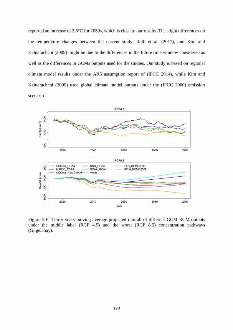
120
reported an increase of 2.6°C for 2050s, which is close to our results. The slight differences on
the temperature changes between the current study, Roth et al. (2017), and Kim and
Kaluarachchi (2009) might be due to the differences in the future time window considered as
well as the differences in GCMs outputs used for the studies. Our study is based on regional
climate model results under the AR5 assumption report of (IPCC 2014), while Kim and
Kaluarachchi (2009) used global climate model outputs under the (IPCC 2000) emission
scenario.
Figure 5-6: Thirty years moving average projected rainfall of different GCM-RCM outputs
under the middle label (RCP 4.5) and the worst (RCP 8.5) concentration pathways
(Gilgelabay).
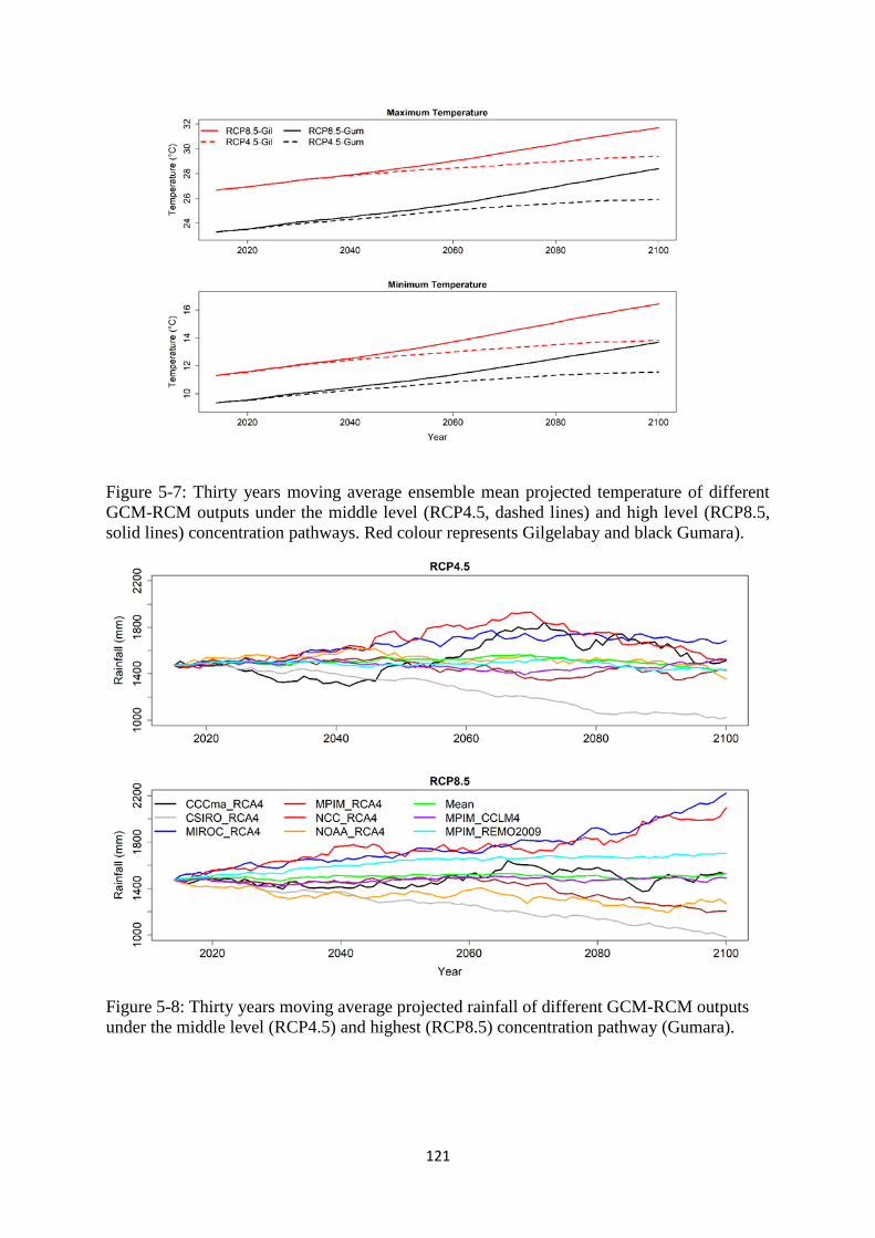
121
Figure 5-7: Thirty years moving average ensemble mean projected temperature of different
GCM-RCM outputs under the middle level (RCP4.5, dashed lines) and high level (RCP8.5,
solid lines) concentration pathways. Red colour represents Gilgelabay and black Gumara).
Figure 5-8: Thirty years moving average projected rainfall of different GCM-RCM outputs
under the middle level (RCP4.5) and highest (RCP8.5) concentration pathway (Gumara).
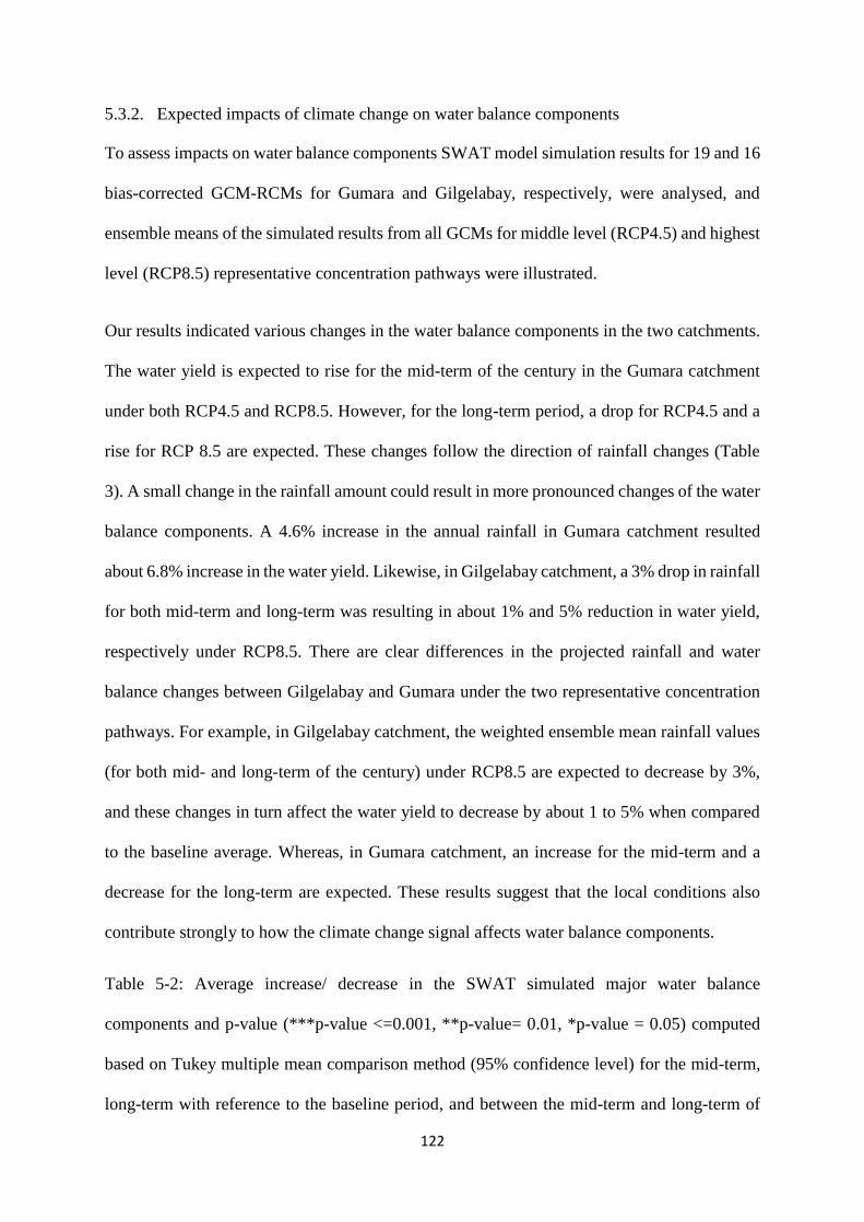
122
5.3.2. Expected impacts of climate change on water balance components
To assess impacts on water balance components SWAT model simulation results for 19 and 16
bias-corrected GCM-RCMs for Gumara and Gilgelabay, respectively, were analysed, and
ensemble means of the simulated results from all GCMs for middle level (RCP4.5) and highest
level (RCP8.5) representative concentration pathways were illustrated.
Our results indicated various changes in the water balance components in the two catchments.
The water yield is expected to rise for the mid-term of the century in the Gumara catchment
under both RCP4.5 and RCP8.5. However, for the long-term period, a drop for RCP4.5 and a
rise for RCP 8.5 are expected. These changes follow the direction of rainfall changes (Table
3). A small change in the rainfall amount could result in more pronounced changes of the water
balance components. A 4.6% increase in the annual rainfall in Gumara catchment resulted
about 6.8% increase in the water yield. Likewise, in Gilgelabay catchment, a 3% drop in rainfall
for both mid-term and long-term was resulting in about 1% and 5% reduction in water yield,
respectively under RCP8.5. There are clear differences in the projected rainfall and water
balance changes between Gilgelabay and Gumara under the two representative concentration
pathways. For example, in Gilgelabay catchment, the weighted ensemble mean rainfall values
(for both mid- and long-term of the century) under RCP8.5 are expected to decrease by 3%,
and these changes in turn affect the water yield to decrease by about 1 to 5% when compared
to the baseline average. Whereas, in Gumara catchment, an increase for the mid-term and a
decrease for the long-term are expected. These results suggest that the local conditions also
contribute strongly to how the climate change signal affects water balance components.
Table 5-2: Average increase/ decrease in the SWAT simulated major water balance
components and p-value (***p-value <=0.001, **p-value= 0.01, *p-value = 0.05) computed
based on Tukey multiple mean comparison method (95% confidence level) for the mid-term,
long-term with reference to the baseline period, and between the mid-term and long-term of
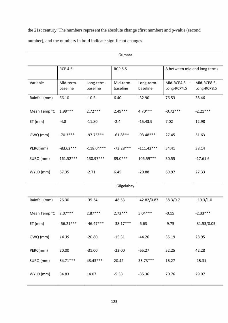
123
the 21st century. The numbers represent the absolute change (first number) and p-value (second
number), and the numbers in bold indicate significant changes.
Gumara
RCP 4.5 RCP 8.5 Δ between mid and long terms
Variable Mid-term-
baseline
Long-term-
baseline
Mid-term-
baseline
Long-term-
baseline
Mid-RCP4.5 –
Long-RCP4.5
Mid-RCP8.5-
Long-RCP8.5
Rainfall (mm) 66.10 -10.5 6.40 -32.90 76.53 38.46
Mean Temp °C 1.99*** 2.72*** 2.49*** 4.70*** -0.72*** -2.21***
ET (mm) -4.8 -11.80 -2.4 -15.43.9 7.02 12.98
GWQ (mm) -70.3*** -97.75*** -61.8*** -93.48*** 27.45 31.63
PERC(mm) -83.62*** -118.04*** -73.28*** -111.42*** 34:41 38.14
SURQ (mm) 161.52*** 130.97*** 89.0*** 106.59*** 30.55 -17.61.6
WYLD (mm) 67.35 -2.71 6.45 -20.88 69.97 27.33
Gilgelabay
Rainfall (mm) 26.30 -35.34 -48.53 -42.82/0.87 38.3/0.7 -19.3/1.0
Mean Temp °C 2.07*** 2.87*** 2.72*** 5.04*** -0.15 -2.33***
ET (mm) -56.21*** -46.47*** -38.17*** -6.63 -9.75 -31.53/0.05
GWQ (mm) 14.39 -20.80 -15.31 -44.26 35.19 28.95
PERC(mm) 20.00 -31.00 -23.00 -65.27 52.25 42.28
SURQ (mm) 64,71*** 48.43*** 20.42 35.73*** 16.27 -15.31
WYLD (mm) 84.83 14.07 -5.38 -35.36 70.76 29.97
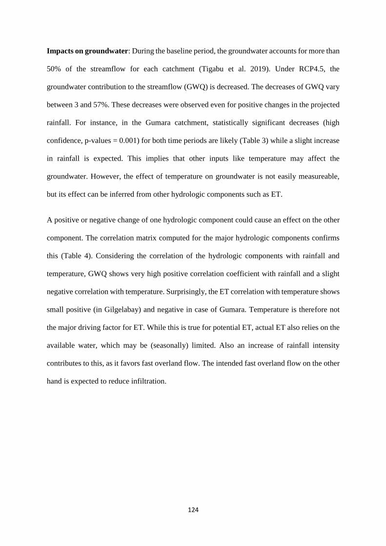
124
Impacts on groundwater: During the baseline period, the groundwater accounts for more than
50% of the streamflow for each catchment (Tigabu et al. 2019). Under RCP4.5, the
groundwater contribution to the streamflow (GWQ) is decreased. The decreases of GWQ vary
between 3 and 57%. These decreases were observed even for positive changes in the projected
rainfall. For instance, in the Gumara catchment, statistically significant decreases (high
confidence, p-values = 0.001) for both time periods are likely (Table 3) while a slight increase
in rainfall is expected. This implies that other inputs like temperature may affect the
groundwater. However, the effect of temperature on groundwater is not easily measureable,
but its effect can be inferred from other hydrologic components such as ET.
A positive or negative change of one hydrologic component could cause an effect on the other
component. The correlation matrix computed for the major hydrologic components confirms
this (Table 4). Considering the correlation of the hydrologic components with rainfall and
temperature, GWQ shows very high positive correlation coefficient with rainfall and a slight
negative correlation with temperature. Surprisingly, the ET correlation with temperature shows
small positive (in Gilgelabay) and negative in case of Gumara. Temperature is therefore not
the major driving factor for ET. While this is true for potential ET, actual ET also relies on the
available water, which may be (seasonally) limited. Also an increase of rainfall intensity
contributes to this, as it favors fast overland flow. The intended fast overland flow on the other
hand is expected to reduce infiltration.
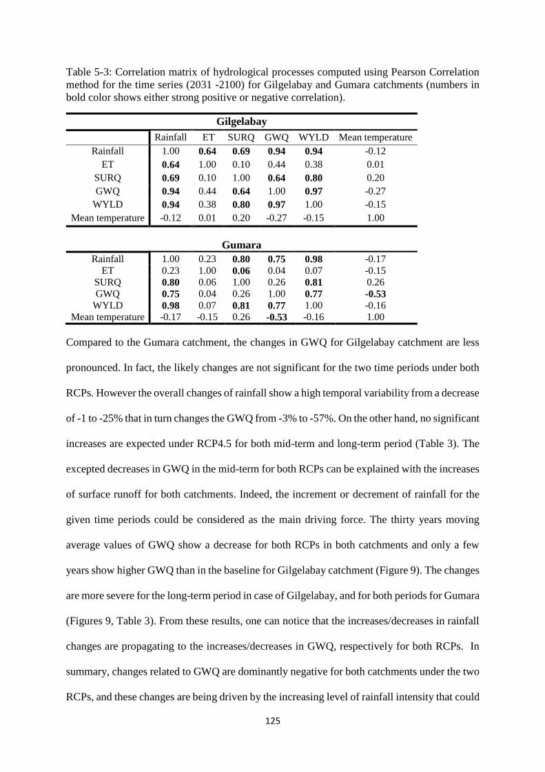
125
Table 5-3: Correlation matrix of hydrological processes computed using Pearson Correlation
method for the time series (2031 -2100) for Gilgelabay and Gumara catchments (numbers in
bold color shows either strong positive or negative correlation).
Gilgelabay
Rainfall ET SURQ GWQ WYLD Mean temperature
Rainfall 1.00 0.64 0.69 0.94 0.94 -0.12
ET 0.64 1.00 0.10 0.44 0.38 0.01
SURQ 0.69 0.10 1.00 0.64 0.80 0.20
GWQ 0.94 0.44 0.64 1.00 0.97 -0.27
WYLD 0.94 0.38 0.80 0.97 1.00 -0.15
Mean temperature -0.12 0.01 0.20 -0.27 -0.15 1.00
Gumara
Rainfall 1.00 0.23 0.80 0.75 0.98 -0.17
ET 0.23 1.00 0.06 0.04 0.07 -0.15
SURQ 0.80 0.06 1.00 0.26 0.81 0.26
GWQ 0.75 0.04 0.26 1.00 0.77 -0.53
WYLD 0.98 0.07 0.81 0.77 1.00 -0.16
Mean temperature -0.17 -0.15 0.26 -0.53 -0.16 1.00
Compared to the Gumara catchment, the changes in GWQ for Gilgelabay catchment are less
pronounced. In fact, the likely changes are not significant for the two time periods under both
RCPs. However the overall changes of rainfall show a high temporal variability from a decrease
of -1 to -25% that in turn changes the GWQ from -3% to -57%. On the other hand, no significant
increases are expected under RCP4.5 for both mid-term and long-term period (Table 3). The
excepted decreases in GWQ in the mid-term for both RCPs can be explained with the increases
of surface runoff for both catchments. Indeed, the increment or decrement of rainfall for the
given time periods could be considered as the main driving force. The thirty years moving
average values of GWQ show a decrease for both RCPs in both catchments and only a few
years show higher GWQ than in the baseline for Gilgelabay catchment (Figure 9). The changes
are more severe for the long-term period in case of Gilgelabay, and for both periods for Gumara
(Figures 9, Table 3). From these results, one can notice that the increases/decreases in rainfall
changes are propagating to the increases/decreases in GWQ, respectively for both RCPs. In
summary, changes related to GWQ are dominantly negative for both catchments under the two
RCPs, and these changes are being driven by the increasing level of rainfall intensity that could
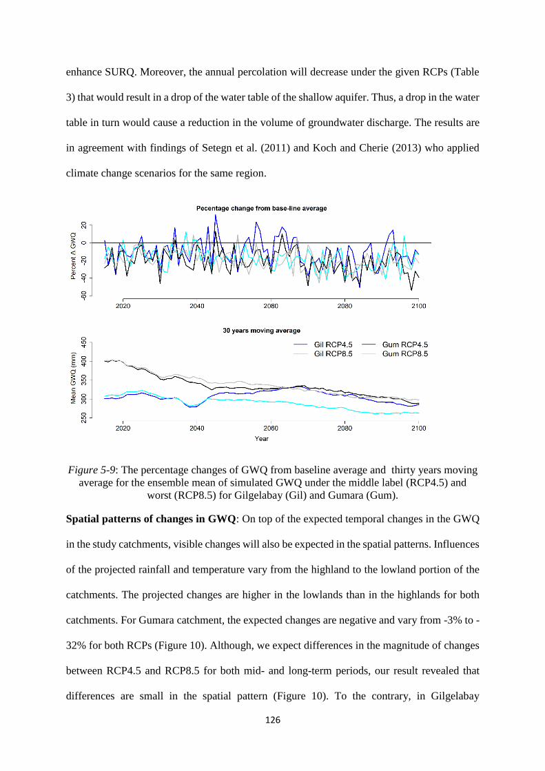
126
enhance SURQ. Moreover, the annual percolation will decrease under the given RCPs (Table
3) that would result in a drop of the water table of the shallow aquifer. Thus, a drop in the water
table in turn would cause a reduction in the volume of groundwater discharge. The results are
in agreement with findings of Setegn et al. (2011) and Koch and Cherie (2013) who applied
climate change scenarios for the same region.
Figure 5-9: The percentage changes of GWQ from baseline average and thirty years moving
average for the ensemble mean of simulated GWQ under the middle label (RCP4.5) and
worst (RCP8.5) for Gilgelabay (Gil) and Gumara (Gum).
Spatial patterns of changes in GWQ: On top of the expected temporal changes in the GWQ
in the study catchments, visible changes will also be expected in the spatial patterns. Influences
of the projected rainfall and temperature vary from the highland to the lowland portion of the
catchments. The projected changes are higher in the lowlands than in the highlands for both
catchments. For Gumara catchment, the expected changes are negative and vary from -3% to -
32% for both RCPs (Figure 10). Although, we expect differences in the magnitude of changes
between RCP4.5 and RCP8.5 for both mid- and long-term periods, our result revealed that
differences are small in the spatial pattern (Figure 10). To the contrary, in Gilgelabay
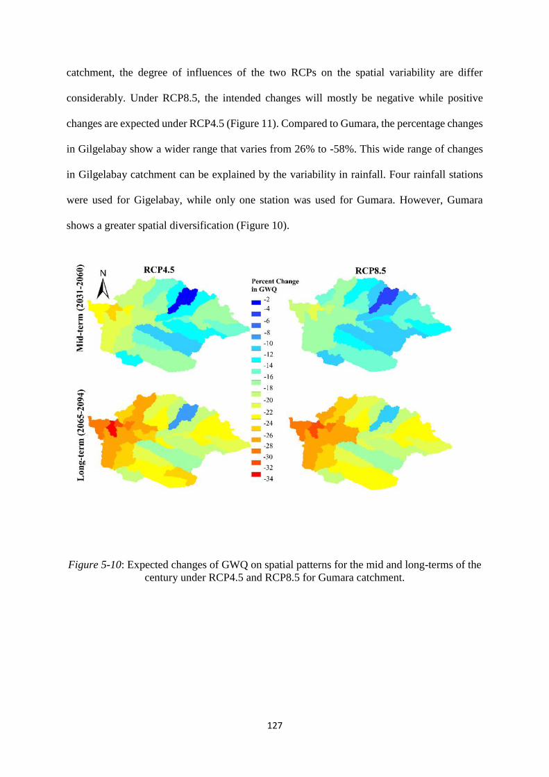
127
catchment, the degree of influences of the two RCPs on the spatial variability are differ
considerably. Under RCP8.5, the intended changes will mostly be negative while positive
changes are expected under RCP4.5 (Figure 11). Compared to Gumara, the percentage changes
in Gilgelabay show a wider range that varies from 26% to -58%. This wide range of changes
in Gilgelabay catchment can be explained by the variability in rainfall. Four rainfall stations
were used for Gigelabay, while only one station was used for Gumara. However, Gumara
shows a greater spatial diversification (Figure 10).
Figure 5-10: Expected changes of GWQ on spatial patterns for the mid and long-terms of the
century under RCP4.5 and RCP8.5 for Gumara catchment.
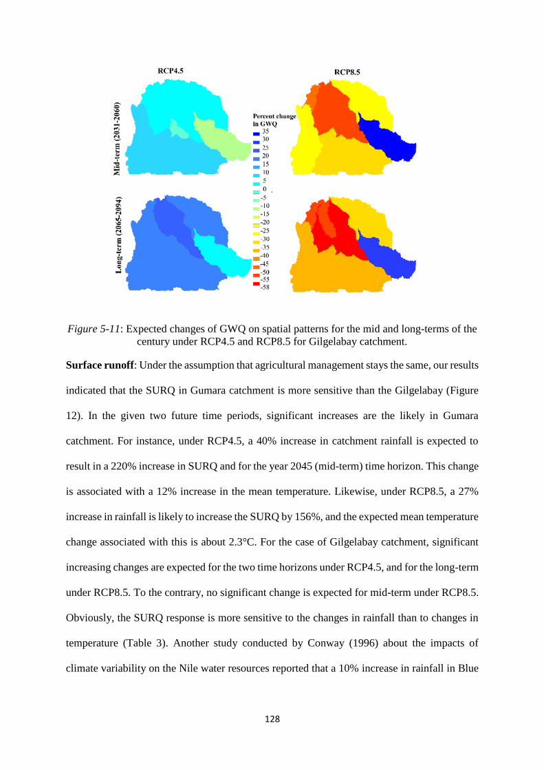
128
Figure 5-11: Expected changes of GWQ on spatial patterns for the mid and long-terms of the
century under RCP4.5 and RCP8.5 for Gilgelabay catchment.
Surface runoff: Under the assumption that agricultural management stays the same, our results
indicated that the SURQ in Gumara catchment is more sensitive than the Gilgelabay (Figure
12). In the given two future time periods, significant increases are the likely in Gumara
catchment. For instance, under RCP4.5, a 40% increase in catchment rainfall is expected to
result in a 220% increase in SURQ and for the year 2045 (mid-term) time horizon. This change
is associated with a 12% increase in the mean temperature. Likewise, under RCP8.5, a 27%
increase in rainfall is likely to increase the SURQ by 156%, and the expected mean temperature
change associated with this is about 2.3°C. For the case of Gilgelabay catchment, significant
increasing changes are expected for the two time horizons under RCP4.5, and for the long-term
under RCP8.5. To the contrary, no significant change is expected for mid-term under RCP8.5.
Obviously, the SURQ response is more sensitive to the changes in rainfall than to changes in
temperature (Table 3). Another study conducted by Conway (1996) about the impacts of
climate variability on the Nile water resources reported that a 10% increase in rainfall in Blue
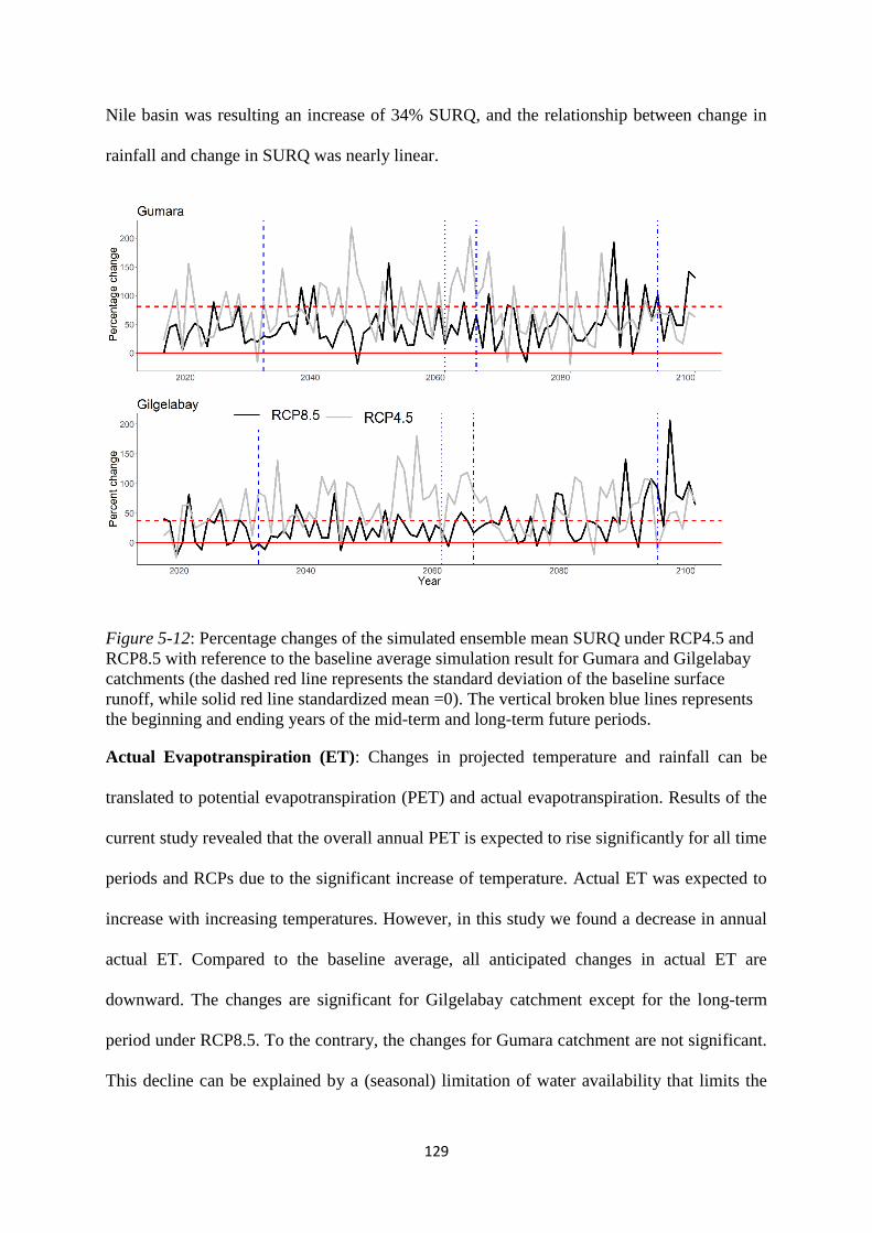
129
Nile basin was resulting an increase of 34% SURQ, and the relationship between change in
rainfall and change in SURQ was nearly linear.
Figure 5-12: Percentage changes of the simulated ensemble mean SURQ under RCP4.5 and
RCP8.5 with reference to the baseline average simulation result for Gumara and Gilgelabay
catchments (the dashed red line represents the standard deviation of the baseline surface
runoff, while solid red line standardized mean =0). The vertical broken blue lines represents
the beginning and ending years of the mid-term and long-term future periods.
Actual Evapotranspiration (ET): Changes in projected temperature and rainfall can be
translated to potential evapotranspiration (PET) and actual evapotranspiration. Results of the
current study revealed that the overall annual PET is expected to rise significantly for all time
periods and RCPs due to the significant increase of temperature. Actual ET was expected to
increase with increasing temperatures. However, in this study we found a decrease in annual
actual ET. Compared to the baseline average, all anticipated changes in actual ET are
downward. The changes are significant for Gilgelabay catchment except for the long-term
period under RCP8.5. To the contrary, the changes for Gumara catchment are not significant.
This decline can be explained by a (seasonal) limitation of water availability that limits the
130
responses to warming (Cordon et al. 2020, Wagner et al., 2015). About 51% of ET takes place
during the dry season (October to May), when less water is available. It is not uncommon to
get less ET in areas where the available water volume is small, and the available water volume
and soil moisture are regularly correlated with rainfall. For the current study, the decreases in
the future ET changes in Gumara and Gilgelabay catchments are limited by the available water.
A significant increase on SURQ, and a significant decrease in the soil moisture content are
expected under both RCPs and time periods that will likely cause less ET. The projected
ensemble mean rainfall datasets, show that the future rainy days are expected to decrease
compared to the number of rainy days during the baseline period even though the expected
changes of total annual rainfall is not significant. In Gumara catchment, the average number of
days with none zero rainfall records was 170 during the baseline period, while 160 and 154
rainy days for the mid-term and long term, respectively. Likewise, in Gilgelabay catchment the
future rainy days are expected to decrease with a slope of 0.03day which is about a drop by 7
to 10 days when compared to the baseline. This indicates that the rainfall intensity is expected
to go up, which in turn causes high surface runoff and less ET. High intensity rainfall may
reduce ET as there will be less water interception and soil moisture content. This can explain
why less ET is simulated even for positive changes of rainfall. Furthermore, ET change rates
differ among catchments depending on the land cover types and different underlying surfaces
processes (Woldesenbet et al. 2017; Wagner et al. 2019). In response to the rises in the mean
temperature, the future PET changes with reference to the baseline average are expected to
increase. This was directly reflected by all PET changes in the two catchments.
5.4. Conclusion
In this study, we investigated the future (2031-2060, 2065- 2094) temporal and spatial changes
of groundwater contribution to streamflow and of major water balance components in two
catchments (Gilgelabay and Gumara) of the Lake Tana basin, in northwestern Ethiopia under
131
RCP4.5 and RCP8.5 using CORDEX datasets (CMPI5). Impacts on water resources were
assessed using the hydrological model SWAT.
The groundwater contribution to streamflow is projected to decline while no or only slight
changes on rainfall are expected. The study catchments are expected to experience decreases
of groundwater contribution to streamflow and increases in surface runoff. Future number of
rainy days are expected to decrease in both catchments under the two concentration pathways.
However, actual ET demand is higher under rising temperature, the anticipated actual ET
would decrease in both catchments due to water limitation.
Compared to the baseline average, the intended changes of groundwater contribution to
streamflow for the mid-term and long-term time period are significant for Gumara, while these
changes are not significant in Gilgelabay catchment under both RCPs. Anticipated changes of
surface runoff will be significant for both catchments during the mid-term and long-term
periods when compared to the baseline period. Comparing results between the mid-term results
and the long-term periods, the differences are expected not to be significant. Only, the annual
ET is expected to be significantly higher during long-term than the mid-term under RCP8.5.
Distinct spatial patterns are expected in the groundwater contribution to streamflow for the two
catchments. The declines of groundwater contribution to streamflow will be higher in lowland
portions of the two catchments than in the highlands.
As this impact assessment study considered multiple GCM-RCMs from the Coupled Model
Intercomparison Project and assessed ensemble results, we believe that the results provide a
range of projections that are relevant for future water management planning in the region.
All anticipated changes in the given hydrological components were modeled under the
assumption that the current agricultural management practices and land cover conditions would
not change. The projection showed that the anticipated future rainfall would be more intense

132
than during the baseline resulting in more surface runoff. Hence, to mitigate climate change
impacts it can be recommended to apply agricultural management practices that enhance
infiltration and lead to an increase of water storage.
133
6. General discussion and conclusion
6.1. General discussion and conclusion
Globally, fresh water resources are under growing pressure due to rising global water demands
of the rapidly growing world population, improved living standards, changed consumption
patterns, and expansion of irrigated agriculture (Mekonnen and Hoekstra 2016). On a global
scale, over 2 billion people live in countries with high water stress representing (11% of the
global average area) (WWAP 2019). Water availability of a country is usually reported as an
annual average value and does not account for seasonal and spatial variability. Ethiopia is one
of the countries with a significant seasonal variation of its water availability. The situation is
critical in the Upper Blue Nile Basin due to inappropriate water management (Polanco et al.
2017; Woldesenbet et al. 2017). Even with an average annual rainfall in the basin of 1800 mm
there is still a considerable water shortage during the dry season (Gebrehiwot et al. 2011).
Were there significant long-term changes (1960-2015) in rainfall, streamflow, and lake
outflow time series observable in the Lake Tana basin?
One of the main purposes of this study was to investigate the temporal variability of the long-
term rainfall, streamflow, and lake outflow records from 1960 to 2015.
Rainfall and discharge patterns
Rainfall time series differed between the stations. The seasonal Mann Kendal (MK) trend test
results indicated that the direction of changes varies between the wet and dry season rainfall.
During the rainy season, about 61% of the rainfall stations considered in this study showed an
upward trend, but only 33% of the changes were significant. For the dry season, 17% of the
stations had a significant decrease and only one station (Mekaneyesu) showed a significant
134
increase. The MK trends of the daily and annual data records were mainly upward but most
were not significant. Overall, 44% were decreasing, 56% increasing, and 78% not significant.
Changes of streamflow (Abay/outflow, Gilgelaabay, Gumara, Megech, and Ribb) and lake
level time series from 1960 to 2014 were analysed. Positive changes were observed for daily
and annual streamflow time series of all catchments, however not all differences were
significant. Only Megech and Gumara showed a significant increase of their annual and
decadal mean values. The outflow from the lake decreased significantly during the 2010s.
Compared to previous studies the overall annual changes in the rainfall were found to be in
agreement with results of Tesemma et al. (2010), Gebremichael et al. (2013), and Tekleab et
al. (2013). All studies agreed that the overall changes of the rainfall in Upper Blue Nile were
not significant from 1964 until 2005. We could also confirm the results of Tekleab et al. (2013)
who reported a significant change for Gumara and no significant increase in streamflow in the
Ribb catchment. For the lake outflow, the current study described a high variability of the
decadal mean outflow from 1960 to 2014 and a non-significant upward change while the ten
years moving average values during the 2010s showed a significant decrease.
Generally, the overall trends of streamflow were upward while no significant changes were
observed for the basin rainfall. This implies that the driver for the changes of streamflow are
land use/cover changes and changes of rainfall intensity. Agriculture has intensified and
urbanization has increased. From 1973 to 2010, an expansion of the cultivated land and a
decline of the woody shrub and forestlands was observed in the Lake Tana basin (Woldesembet
et al. 2017). Similarly, Gashaw & Fentahun (2014) reported an increase on both cultivation
land and land degradation in the Eastern Lake Tana basin. Another study carried out in the
Gumara catchment by Wubie et al. (2016) addressed the land use/cover changes over two
consecutive periods (1957–1985 and 1985–2005), they found considerable land use changes,
135
i.e. natural forests and wetland were converted to cultivated land and settlements. Gebremicael
et al. (2013) confirmed that land use change has caused a significant increase of runoff and
sediment load in the Upper Blue Nile during the last four decades. Those changes can enhance
surface runoff by decreasing the infiltration rates. Moreover, the long-term rainfall records
showed a decreasing trend of the number of rainy days in a year, while the total annual rainfall
remains unchanged (Teshome et al. 2016). Changing rainfall properties like duration, intensity,
and inter-event durations in the Blue Nile basin are also assumed to be an important reason for
a change in streamflow in the region (Haile et al. 2010).
In summary, the hydrologic regime of the Lake Tana basin is changing overtime because of
the significant changes on the land use pattern. However, rainfall changes were not significant.
How do the major water balance components vary on spatial and seasonal basis under
different agricultural crops and land use/cover classes?
The major economic activity in the Lake Tana basin is agriculture with different crops. We
analyzed changes of the major water balance components between dry and wet seasons, and
between the three catchments (Gilgelabay, Gumara, and Ribb) caused by different agricultural
crops and other land use/cover classes and their spatial and seasonal variation
Changes in land use/cover alter surface roughness, albedo and other properties of a catchment,
which in turn cause variability in the hydrological processes by changing the energy exchange
between the atmosphere and land surface and net radiation (Luo et al. 2016). In the Lake Tana
Basin, this study also shows changes in the hydrology due to different land use/covers.
Groundwater recharge: comparing the rate of groundwater recharge from agricultural crops
and other land use/covers, we find that cereal crops like millet, teff, wheat, and barley show
relatively higher recharge rates as compared to mixed crops, pulses, rice, grassland, and forest.
136
The changes on groundwater recharge are also reflected on the spatial patterns indicating
variable effects of different land uses. Results show significantly higher GW recharge rate for
agricultural areas than forest cover ones. These differences of the groundwater recharge rate
among different LULC classes could be caused by the variability of the soil structure, water
interception and transpiration demand of different vegetation covers. Agricultural activities can
also increase infiltration due to tillage of the soil (Gumindoga et al. 2014).
Surface runoff: the surface runoff also shows considerable variability among the different land
use classes and between the three catchments. Results show that hydrologic response units
(HRUs) that include medium density urban settlements, farm settlements, and mixed cropland
as the land use/cover class increased the magnitude of surface runoff. The differences in its
magnitude vary significantly from one land use class to another one. Compared to other land
use classes, the annual mean runoff magnitude on corn cover area is above all other land use
classes. The differences vary from 14 mm to 83 mm and all are significant. Contrary to this,
cereal crops such as teff, wheat, and barely show relatively low runoff. These differences can
be explained by the lower runoff curve number value in the case of cereal and vice-versa in the
case of corn. When we consider the effect runoff between the three catchments, our results
show that Gumara catchment is the most vulnerable one followed by Ribb.
Actual evapotranspiration (ET): similar to groundwater recharge, ET also varies among
different land use/cover classes. The annual mean values decrease from forest cover to
agricultural land for all the three catchments. Among the agricultural crop, teff has the smallest
amounts of average annual water loss by ET. The differences in ET values among the different
crops and other land use classes could be a result of differences in water uptake, available water
capacity, and leaf area indices.
137
Apart from changes of HRUs, the water balance components reflect the patterns of the rainfall
distribution in the Gilgelabay catchment. The northern and south-western part of the catchment
are characterized by high amount of groundwater recharge and surface runoff, as a result of the
highest amount of rainfall in the catchment (Figure 3.5, 3.7, and 3.9). In the Gumara and Ribb
catchments the spatial variation of the water balance components are not influenced by rainfall
as only one rainfall station was used for the simulation, so that LULC and soil units have more
influence on the spatial patterns of hydrologic components than rainfall. We found also
significant seasonal variability of the hydrologic components. Because of the influence of the
ITCZ position, about 80% of the rainfall falls during the summer (wet season), and this controls
water availability in the catchments. More than 90% of the groundwater recharge and surface
runoff and about 49% of the ET take place during the wet season. Therefore, the seasonal
anomalies on the recharge and surface runoff processes in the region are largely correlated to
the rainfall anomalies between the dry and wet seasons, while the overall ET variability
between the two seasons is not pronounced. Base flow has substantial contribution to
streamflow of the Lake Tana Basin.
In all the three catchments streamflow is dominated by base flow. Setegn et al. (2008) also
found that the base flow contribution to streamflow is very high. However, there are differences
between this study and Setegn et al. (2008). For example, Setegn et al. (2008) reported a 59%
base flow contribution for Gilgelabay catchment, while 73% is found in the current study.
Because of the differences of fitted model parameters between the three catchments, the base
flow contribution to the streamflow varies.
In conclusion, this study proved that hydrologic processes (groundwater recharge, surface
runoff, actual evapotranspiration) are significantly varying between cereal crops, leguminous
plants, grassland, and forest covers. As an example, the degree of vulnerability to surface runoff
is the highest in Gumara, and groundwater recharge is highest in Gilgelabay catchment. The
138
differences are weaker between the Gumara and Ribb catchments. Furthermore, the
groundwater recharge, water yield, and surface runoff values varied between the dry and wet
seasons in the three catchments.
Do the groundwater and surface water systems interact with each other and how does the
behavior of GW-SW interaction vary in space and time?
By applying the SWAT model (Arnold et al. 1998; Arnold and Fohrer 2005) we found that
groundwater has significant contribution to streamflow. However, we could not fully explain
the bidirectional groundwater (GW)–surface water (SW) interaction. Moreover, the spatio-
temporal flow dynamics of the groundwater were not addressed sufficiently. GW-SW
interactions and the resulting exchange fluxes are often characterised by a high temporal and
spatial variability (Krause et al. 2007). Therefore, we used a coupled GW-SW hydrologic
model (SWAT-MODFLOW) (Bailey et al. 2016) to gain new insights into the spatio-temporal
flow dynamics of groundwater-surface water interactions.
In this section we analyze the hydraulic connection between the aquifer and stream network,
the spatio-temporal variation of GW-SW interactions and the differences of the GW-SW
interaction between the three catchments.
The model efficiencies of the measured monthly streamflow are very good (NS >0.7) for all
the three catchments (Table 4.1). Results showed that GW-SW interactions varied both on
space and time. Groundwater recharge zones are mainly located in the highland areas. The
potential head difference between the aquifer and the stream and other properties such as
hydraulic conductivity, specific storage and initial groundwater head are the main controlling
factors for the spatial variability of GW-SW interaction (Kim et al. 2008). The current study
found most interactions between the GW and SW during the wet season. This high variability
of the GW-SW interaction between the dry and wet months influences the water level in the
139
rivers. The dominant exchange is 170 (m3/day) from the aquifer to the stream system in the
Gilgelaby catchment.
In Gumara and Ribb the exchange between aquifer and stream is bidirectional for all time steps.
The Gumara catchment is largely controlled by the surrounding surface water system. In the
downstream floodplain and reaches groundwater is discharged to the stream system (Figure
4.5). Dessie et al. (2014) reported that the floodplain of the Gumara catchment was recharged
by the groundwater during the rainy season. Chebud and Melesse (2009) also reported that 0.09
billion cubic meter of water flow out of from floodplain aquifer to the Lake Tana during the
wet season. The bidirectional flow of the Ribb catchment is more or less similar to the Gumara
catchment. Since the early 1990s the temporal patterns showed significant changes for the
entire year and during the dry season (magnitude and flow direction) for the two catchments
(Figure 4.4, 4.5). Before the early 1990s the flow direction was from the stream to the aquifer
and changed later. This decrease of flow from the river network to the aquifer and the change
of direction from the aquifer to the stream system (annual and dry season) over time could be
related to the increase of runoff. Recently the number of rainy days in a year are decreasing
while the total rainfall amount did not change significantly, which in turn leads to more
intensive rainfall and results in more surface runoff generation and less seepage to the aquifer
system. Another notable result from this investigation is the strong dynamics of the exchange
fluxes between the aquifer and the stream system on the daily time step (Figure 4.3). The high
variability of the daily and seasonal GW-SW exchange rates might be attributed to a large
variation in daily rainfall (coefficient of variation ranging from 100 to 200%) (refer to section
4.3.1).
Overall, we found a strong hydraulic connection between GW-SW systems and all the three
catchments are characterized by a considerable spatio-temporal variability within and between
the catchments. The annual temporal patterns and direction of the water fluxes in the
140
Gilgelabay catchment differs from the ones in the Gumara and Ribb catchments where
negligible seepage from the stream was found.
How will future climate change affect the major water balance components of the Lake
Tana basin?
After the discussion of historical and current hydrologic conditions, in the following possible
future changes of the major hydrologic components for two climate change scenarios are
discussed for the mid-term (2031-2060) and long-term (2065-2094).
The mean annual temperature is expected to increase significantly while the ensemble annual
mean rainfall from 19 (Gumara) and 16 (Gilgelabay) regional climate models shows only minor
changes for the mid-term and long-term compared to the baseline period from 1985 to 2014.
Impact on water balance: With rising temperatures, one may expect more potential
evapotranspiration (PET) and actual evapotranspiration (ET), which in turn could cause a drop
of the groundwater contribution (GWQ) to the streamflow. Here, we analyse the model results
for the major water balance components with the Mann Kendall trend test and the Tukey
multiple mean comparison tests applied on the annual values of each hydrologic component.
The future annual mean temperature is expected to rise significantly (p-value<0.05) for both
time windows and RCPs, which in turn will cause a significant increase of PET. To the
contrary, our results show a decrease of the annual ET. Nevertheless, the projected declines are
not statistically significant for Gumara, while the decrease is significant for the Gilgelabay
catchment (Table 5.2). The GWQ is also anticipated to drop significantly (p-value<0.05) in
Gumara, while no significant (p-value>0.05) decrease is expected in Gilgelabay except for the
mid-term of RCP4.5. Significant increases will be expected for SURQ in both catchments. The
expected changes of surface runoff are positive even under conditions of slightly lower rainfall.
But the number of projected rainy days will decrease in both catchments. Future rainfall is
141
expected to be more intense than the rainfall during the baseline period. As a result, more
surface runoff will be expected. Thus, the expected increase of runoff will have different
implications on the other water balance components. Except for the mid-term of RCP4.5 in
Gilgelabay, the groundwater contribution to the streamflow is expected to decrease for both
catchments and both RCPs. The decrease in the Gumara catchment is significant, whereas it is
not significant in Gilgelabay. ET was expected to increase with increasing temperatures.
However, we found a decrease of ET in both catchments. This decline was observed even for
positive changes of the projected rainfall because water availability limited the responses to
warming (Condon et al. 2020, Wagner et al., 2015). About 51% of ET takes place during the
dry season (October to May), when less water is available. These decreases of ET and GWQ
highlight that the larger increase on SURQ limits the availability of water for other hydrologic
processes. Expected changes of water yield will not be significant as the increase of surface
runoff will be compensated by the decrease of GWQ and for both catchments. Moreover, we
found a decrease of annual percolation and soil moisture that could result in a drop of the water
table of the shallow aquifer. Thus, a decrease of the water table and soil moisture in turn would
cause a reduction of the groundwater discharge and evapotranspiration. Setegn et al. (2011)
also reported a decrease on the future GWQ under A1B and B scenarios outputs from GFDL
and MPI.
In general, the small changes on rainfall in the scenario data will result in a significant change
of the major hydrologic components. The temperature effect seems smaller than the rainfall
effect. However, potential evapotranspiration (PET) is significantly higher under the two
RCPs.
Spatial patterns of changes in GWQ: The impact of climate change is variable in space.
Effects of rainfall and temperature changes on GWQ vary from the highlands to the lowlands
142
in the two catchments with more pronounced effects in the lowlands than in the highlands
(Figure 5.10, 5.11). For the Gumara catchment we expect a decrease for the two future time
periods and a slight increase for the mid-term period under RCP4.5 in Gilgelabay catchment.
The differences between the two catchments could be related to the different local climates,
static factors such as topography and slope.
Overall, the significant increase of the projected temperature and the small changes of the
rainfall amount and intensity are expected to change the major water balance components.
Surface runoff and groundwater contribution to the streamflow are expected to change in
opposite directions. Here, increased surface runoff primarily contributes to a reduction of
groundwater contribution to the streamflow.
6.2. General Conclusion
This PhD thesis provides an additional understanding and new information about the past,
present, and future hydrologic perspectives of the Lake Tana Basin. The topics covered
includes statistical analyses of hydrometeorological time series, impacts of agricultural crops
on hydrology, groundwater and surface water interaction, and impact of climate change on
water resource in the Lake Tana Basin. The physically based hydrologic models SWAT and
SWAT-MODFLOW were set up to model the past, the present and future hydrologic
components in the Lake Tana basin. The models were calibrated and validated with measured
streamflow data from the three catchments with satisfactory results. The key findings are:
Long-term hydrometeorological data analyses provide insight into the spatial and temporal
patterns of the climate and hydrologic variables of the past and the results can be useful for
managing possible the future impacts. From the statistical point of view, the hydrologic
behaviour of the study area is highly variable in space and time. The rainfall and streamflow
changes over time vary among annual, dry and wet seasons as well as daily rainfall and
143
streamflow. Historical rainfall records from 1960-2015 showed annual rainfall changes were
not statistically significant for the whole catchment, but many single rainfall stations showed
significant changes of the seasonal values. Unlike the annual rainfall records, streamflow time
series revealed considerable changes on decadal time steps.
The models SWAT and SWAT-MODFLOW help to understand the spatial and seasonal
patterns of the hydrologic components under different land cover/use and climate change
conditions. Modelled results revealed a substantial contribution of groundwater to the
hydrologic systems in the three catchments. Moreover, the different agricultural crops had
different influence on spatial and seasonal patterns of hydrological variables. Some of them
like cereal crops enhanced groundwater recharge, while others such as leguminous plants
favoured surface runoff. Therefore, the future water availability could also be affected by the
types of cultivated crops.
The coupled hydrologic models indicated that the surface water and groundwater systems
interacted with each other with a high spatio-temporal variability. The anomalies were
significantly higher on daily time step than monthly or yearly. However, this coupled model
was not used for climate change impact study due to its high computational run time demand
of the model to get the desired output. We used an ensemble average of 35 rainfall and
temperature outputs from 35 regional climate model to minimize uncertainties associated with
individual RCM (Kling et al. 2012). Due to this, use of the coupled hydrologic model was not
feasible under the given time frame.
Understanding the availability of water resources under global climate change conditions can
provide new insights for policy makers and water managers. This study therefore simulates
different climate scenarios for the study region. Our intention was to understand how the major
water balances components respond to future rainfall and temperature changes. The mean
144
temperature is expected to rise higher than the global average, while the rainfall is not expected
to change significantly. We found that, the groundwater contribution to the streamflow and
actual evapotranspiration tend to decrease whereas the surface runoff is likely to increase.
Hence, appropriately accounting for the major water balance components in the context of
climate change is of great importance when considering the future management and planning
of water resources. Secondly, it is highly advisable to take appropriate measures to mitigate
climate change impacts, e.g. implement water conservation measures, to store the expected
increase of surface runoff and minimize soil erosion.
Overall, the hydrologic modeling methods and results that were based on specific agricultural
crop cover and different climate options have diverse applicability for similar areas worldwide
that are dominantly influenced by agricultural crops to design proper future water management
plans. Moreover, results from the coupled hydrologic model also enhance our level of
understanding on the flow dynamics of groundwater and surface water interaction on different
temporal scales in the current study area and it helps to explain the interconnected hydrologic
processes on other catchments in Ethiopia and Africa. Thus, the methodological approaches
followed in this study could be transferred to such other regions.
Use of hydrological research outputs for decision making processes requires understanding
the level of uncertainty associated with applied research methodology, quality and available
input data, and hydrologic model parameters. Uncertainties associated with hydrologic
modeling results in data scarce regions like that of the current study area are expected to be
high level. Maximum effort was put to minimize uncertainties associated with the hydrologic
model parameters through model calibration and validation using the available limited data.
Nevertheless, we believe that further improvement could be possible by enhancing the database
145
system through regular measurement of groundwater table elevation, withdrawal and stream
stage values.
In general, this study proved that the hydrology of the region was changed overtime due to
escalations of agriculture, which in turn was derived by the rapid population growth. These
changes are expected to be amplified in the future due to climate change unless appropriate
agricultural practice and water resources management are designed to cope up with the
anticipated changes. In this research, crop types were identified according to their impact on
groundwater recharge, surface runoff generation, and evaporative demands, which would be a
good insight to design proper future agricultural and water management practices in the study
region and other similar areas that are under the pressure of intensive agriculture. The
hydrologic models were developed considering agricultural crop variability considering their
topographic variations and growing suitability of individual crops and finally came up with
significance variances of influences on the hydrologic cycle. Thus, it is suggested to transfer
this methodological approach to similar regions that are under rapid population growing
pressure and agricultural intensification.
6.3. A look forward
More than three million inhabitants of the Lake Tana basin put a high pressure on the water
resource in the basin. This research tried to address hydrologic changes of the past, present and
anticipated future in the basin. One key aspect considered was anticipated hydrological changes
under global warming. Our results revealed that groundwater discharge is expected to decrease
whereas surface runoff is expected to increase. However, still groundwater is the only reliable
source of water for domestic, agricultural and industrial uses in the larger part of basin,
especially in the rural area. Consequently, value of groundwater is expected to increase in the
coming future as population is rapidly growing in the region. Therefore, future water

146
management and planning should consider combined use of surface water and groundwater.
To come up with reliable management plans, scientific research outputs are required. Among
others, detail investigation of groundwater-surface water flow dynamics by considering, rate
of water withdrawal, temporal variability of groundwater table, soil moisture, surface water,
and associated extreme condition is still required. Thus, the future research direction could be
coupled model application and extreme flow analysis based on regularly measured data.
147
References
Abate, M., Nyssen, J., Steenhuis, T.S., Moges, M.M., Tilahun, S.A., Enku, T. and Adgo, E.,
2015. Morphological changes of Gumara River channel over 50 years, upper Blue
Nile basin, Ethiopia. Journal of Hydrology, 525, pp.152-164.
Abbaspour, K.C., Vejdani, M., Haghighat, S. and Yang, J., 2007, December. SWAT-CUP
calibration and uncertainty programs for SWAT. In MODSIM 2007 international
congress on modelling and simulation, modelling and simulation society of Australia
and New Zealand (pp. 1596-1602).
Abbaspour, K.C., Rouholahnejad, E., Vaghefi, S.R.I.N.I.V.A.S.A.N.B., Srinivasan, R., Yang,
H. and Kløve, B., 2015. A continental-scale hydrology and water quality model for
Europe: Calibration and uncertainty of a high-resolution large-scale SWAT model.
Journal of Hydrology, 524, pp.733-752.
Abdo, K.S., Fiseha, B.M., Rientjes, T.H.M., Gieske, A.S.M. and Haile, A.T., 2009.
Assessment of climate change impacts on the hydrology of Gilgel Abay catchment in
Lake Tana basin, Ethiopia. Hydrological Processes: An International Journal, 23(26),
pp.3661-3669.
Abera, W., Tamene, L., Abegaz, A. and Solomon, D., 2019. Understanding climate and land
surface changes impact on water resources using Budyko framework and remote
sensing data in Ethiopia. Journal of Arid Environments, 167, pp.56-64.
Adem, A.A., Tilahun, S.A., Ayana, E.K., Worqlul, A.W., Assefa, T.T., Dessu, S.B. and
Melesse, A.M., 2016. Climate change impact on sediment yield in the Upper Gilgel
Abay catchment, Blue Nile Basin, Ethiopia. In Landscape dynamics, soils and
hydrological processes in varied climates (pp. 615-644). Springer, Cham.
ADSWE (Amhara Design and Surevision Works Entreprise), 2017. Spatial data of land use
and soil at the scale of 1: 50,000. Bahir Dar.
Ahring, T.S. and Steward, D.R., 2012. Groundwater surface water interactions and the role of
phreatophytes in identifying recharge zones. Hydrology and Earth System Sciences,
16(11), pp.4133-4142.
Alemayehu, T., McCartney, M. and Kebede, S., 2009. Simulation of water resource
development and environmental flows in the Lake Tana Subbasin. Improved Water
and Land Management in the Ethiopian Highlands: Its Impact on Downstream
Stakeholders Dependent on the Blue Nile, p.23.
148
Alemayehu, T., McCartney, M. and Kebede, S., 2010. The water resource implications of
planned development in the Lake Tana catchment, Ethiopia. Ecohydrology &
Hydrobiology, 10(2), pp.211-221.
Ali, R., McFarlane, D., Varma, S., Dawes, W., Emelyanova, I., Hodgson, G. and Charles, S.,
2012. Potential climate change impacts on groundwater resources of south-western
Australia. Journal of Hydrology, 475, pp.456-472.
AWWCE (Amhara Water Works Constraction Entreprise) , 2016. Well drilling well-log, well
development, pumping test and completion reports of existing water scheme in the
Lake Tana basin. Bahir Dar, Ethiopia.
Arnold, J.G., Srinivasan, R., Muttiah, R.S. and Williams, J.R., 1998. Large area hydrologic
modeling and assessment part I: model development 1. JAWRA Journal of the
American Water Resources Association, 34(1), pp.73-89.
Arnold, J.G. and Fohrer, N., 2005. SWAT2000: current capabilities and research
opportunities in applied watershed modelling. Hydrological Processes: An
International Journal, 19(3), pp.563-572.
Arora, M., Kumar, R., Malhotra, J. and Kumar, N., 2014. Correlations of Stream Flow and
Climatic Variables for a Large Glacierized Himalayan Basin. Journal of Water
Resource and Protection, 6(14), p.1326.
Asfaw, A., Simane, B., Hassen, A. and Bantider, A., 2017. Variability and time series trend
analysis of rainfall and temperature in northcentral Ethiopia: A case study in Woleka
sub-basin. Weather and Climate Extremes.
Arsiso, B.K., Tsidu, G.M., Stoffberg, G.H. and Tadesse, T., 2017. Climate change and
population growth impacts on surface water supply and demand of Addis Ababa,
Ethiopia. Climate Risk Management, 18, pp.21-33.
Bachmair, S. and Weiler, M., 2012. Hillslope characteristics as controls of subsurface flow
variability. Hydrology and Earth System Sciences, 16(10), p.3699.
Bailey, R.T., Wible, T.C., Arabi, M., Records, R.M. and Ditty, J., 2016. Assessing regional‐
scale spatio‐temporal patterns of groundwater–surface water interactions using a
coupled SWAT‐MODFLOW model. Hydrological Processes, 30(23), pp.4420-4433.
Bailey, R., Rathjens, H., Bieger, K., Chaubey, I. and Arnold, J., 2017. SWATMOD‐Prep:
Graphical user interface for preparing coupled SWAT‐MODFLOW simulations.
JAWRA Journal of the American Water Resources Association, 53(2), pp.400-410.
Bates, D.M., 2010. lme4: Mixed-effects modeling with R. Springer Page:, Madison, WI,
USA
149
Berg, P., Feldmann, H. and Panitz, H.J., 2012. Bias correction of high resolution regional
climate model data. Journal of Hydrology, 448, pp.80-92.
Berhanu, B., Seleshi, Y. and Melesse, A.M., 2014. Surface water and groundwater resources
of Ethiopia: potentials and challenges of water resources development. In Nile River
Basin (pp. 97-117). Springer, Cham.
Berihun, M.L., Tsunekawa, A., Haregeweyn, N., Meshesha, D.T., Adgo, E., Tsubo, M.,
Masunaga, T., Fenta, A.A., Sultan, D., Yibeltal, M. and Ebabu, K., 2019.
Hydrological responses to land use/land cover change and climate variability in
contrasting agro-ecological environments of the Upper Blue Nile basin, Ethiopia.
Science of The Total Environment, 689, pp.347-365.
Beyene, T., Lettenmaier, D.P. and Kabat, P., 2010. Hydrologic impacts of climate change on
the Nile River Basin: implications of the 2007 IPCC scenarios. Climatic change,
100(3-4), pp.433-461.
Birsan, M.V., Molnar, P., Burlando, P. and Pfaundler, M., 2005. Streamflow trends in
Switzerland. Journal of hydrology, 314(1-4), pp.312-329.
Björklund, G., 2001. Water management in developing countries-policy and priorities for EU
development cooperation. SIWI report, 12.
Bovolo, C.I., Parkin, G. and Sophocleous, M., 2009. Groundwater resources, climate and
vulnerability. Environmental Research Letters, 4(3), p.035001.
Brookes, J.D. and Carey, C.C., 2015. Ensure availability and sustainable management of
water and sanitation for all. UN Chronicle, 51(4), pp.15-16.
Change, I.C., 2014. Mitigation of climate change. Contribution of working group III to the
fifth assessment report of the intergovernmental panel on climate change. Cambridge,
United Kingdom and New York, USA.
Chatfield, C., 2004. The analysis of time series: an introduction Sixth Edit., Boca Raton
London New York, Washington DC: Chapman and Hall/CRC.
Chebud, Y.A. and Melesse, A.M., 2009. Numerical modeling of the groundwater flow system
of the Gumera sub‐basin in Lake Tana basin, Ethiopia. Hydrological Processes: An
International Journal, 23(26), pp.3694-3704.
Chenhua, S., 2015. Analysis of detrended time-lagged cross-correlation between two
nonstationary time series. Physics Letters A, 379(7), pp.680-687.
Chunn, D., Faramarzi, M., Smerdon, B. and Alessi, D.S., 2019. Application of an Integrated
SWAT–MODFLOW Model to Evaluate Potential Impacts of Climate Change and
150
Water Withdrawals on Groundwater–Surface Water Interactions in West-Central
Alberta. Water, 11(1), p.110.
Comino, J.R., Iserloh, T., Lassu, T., Cerdà, A., Keestra, S.D., Prosdocimi, M., Brings, C.,
Marzen, M., Ramos, M.C., Senciales, J.M. and Sinoga, J.R., 2016. Quantitative
comparison of initial soil erosion processes and runoff generation in Spanish and
German vineyards. Science of the Total Environment, 565, pp.1165-1174.
Condon, L.E., Atchley, A.L. & Maxwell, R.M., 2020. Evapotranspiration depletes
groundwater under warming over the contiguous United States. Nat Commun 11, 873.
https://doi.org/10.1038/s41467-020-14688-0
Conway, D. and Hulme, M., 1993. Recent fluctuations in rainfall and runoff over the Nile
sub-basins and their impact on main Nile discharge. Climatic change, 25(2), pp.127-
151.
Conway, D., 1996. The impacts of climate variability and future climate change in the Nile
Basin on water resources in Egypt. International Journal of Water Resources
Development, 12(3), pp.277-296.
Costa, K., Russell, J., Konecky, B., & Lamb, H., 2014. Isotopic reconstruction of the African
Humid Period and Congo Air Boundary migration at Lake Tana, Ethiopia. Quaternary
Science Reviews, 83, pp.58–67.
Cuthbert, M.O., Gleeson, T., Moosdorf, N., Befus, K.M., Schneider, A., Hartmann, J. and
Lehner, B., 2019a. Global patterns and dynamics of climate–groundwater interactions.
Nature Climate Change, 9(2), p.137.
Cuthbert, M.O., Taylor, R.G., Favreau, G., Todd, M.C., Shamsudduha, M., Villholth, K.G.,
MacDonald, A.M., Scanlon, B.R., Kotchoni, D.O.V., Vouillamoz, J.M. and Lawson,
F.M.A., 2019b. Observed controls on resilience of groundwater to climate variability
in sub-Saharan Africa. Nature, 572(7768), p.230.
Dargahi, B. and Setegn, S.G., 2011. Combined 3D hydrodynamic and watershed modelling
of Lake Tana, Ethiopia. Journal of hydrology, 398(1), pp.44-64.
Chunn, D., Faramarzi, M., Smerdon, B. and Alessi, D.S., 2019. Application of an integrated
SWAT–MODFLOW model to evaluate potential impacts of climate change and water
withdrawals on groundwater–Surface water interactions in West-Central Alberta.
Water, 11(1), p.110.
De Graaf, I.E.M., Van Beek, L.P.H., Wada, Y. and Bierkens, M.F.P., 2014. Dynamic
attribution of global water demand to surface water and groundwater resources:
151
Effects of abstractions and return flows on river discharges. Advances in water
resources, 64, pp.21-33.
Dersseh, M.G., Kibret, A.A., Tilahun, S.A., Worqlul, A.W., Moges, M.A., Dagnew, D.C.,
Abebe, W.B. and Melesse, A.M., 2019. Potential of Water Hyacinth Infestation on
Lake Tana, Ethiopia: A Prediction Using a GIS-Based Multi-Criteria Technique.
Water, 11(9), p.1921.
Dessie, M., Verhoest, N.E., Pauwels, V.R., Adgo, E., Deckers, J., Poesen, J. and Nyssen, J.,
2015. Water balance of a lake with floodplain buffering: Lake Tana, Blue Nile Basin,
Ethiopia. Journal of Hydrology, 522, pp.174-186.
Déqué, M., Rowell, D.P., Lüthi, D., Giorgi, F., Christensen, J.H., Rockel, B., Jacob, D.,
Kjellström, E., De Castro, M. and van den Hurk, B.J.J.M., 2007. An intercomparison
of regional climate simulations for Europe: assessing uncertainties in model
projections. Climatic Change, 81(1), pp.53-70.
Dile, Y.T., Berndtsson, R. and Setegn, S.G., 2013. Hydrological response to climate change
for Gilgelabay river, in the Lake Tana basin-upper blue Nile basin of Ethiopia. PloS
one, 8(10).
Dile, Y.T., Rockström, J. and Karlberg, L., 2016. Suitability of water harvesting in the Upper
Blue Nile Basin, Ethiopia: A first step towards a mesoscale hydrological modeling
framework. Advances in Meteorology, 2016.
Dile, Y.T., Tekleab, S., Ayana, E.K., Gebrehiwot, S.G., Worqlul, A.W., Bayabil, H.K.,
Yimam, Y.T., Tilahun, S.A., Daggupati, P., Karlberg, L. and Srinivasan, R., 2018.
Advances in water resources research in the Upper Blue Nile basin and the way
forward: A review. Journal of hydrology, 560, pp.407-423.
Döll, P., 2009. Vulnerability to the impact of climate change on renewable groundwater
resources: a global-scale assessment. Environmental Research Letters, 4(3), p.035006.
Duvert, C., Jourde, H., Raiber, M. and Cox, M.E., 2015. Correlation and spectral analyses to
assess the response of a shallow aquifer to low and high frequency rainfall
fluctuations. Journal of Hydrology, 527, pp.894-907.
Ebrahim, G.Y., Jonoski, A., van Griensven, A. and Di Baldassarre, G., 2013. Downscaling
technique uncertainty in assessing hydrological impact of climate change in the Upper
Beles River Basin, Ethiopia. Hydrology Research, 44(2), pp.377-398.
Eckhardt, K. and Arnold, J.G., 2001. Automatic calibration of a distributed catchment model.
Journal of hydrology, 251(1-2), pp.103-109.
152
Ehtiat, M., Mousavi, S.J. and Srinivasan, R., 2018. Groundwater modeling under variable
operating conditions using SWAT, MODFLOW and MT3DMS: A catchment scale
approach to water resources management. Water resources management, 32(5),
pp.1631-1649.
Elshamy, M., Seierstad, I.A. and Sorteberg, A., 2009. Impacts of climate change on Blue Nile
flows using bias-corrected GCM scenarios. Hydrol. Earth Syst. Sci., 13, pp.551–565,
2009.
Ely, D.M. and Kahle, S.C., 2012. Simulation of groundwater and surface-water resources and
evaluation of water-management alternatives for the Chamokane Creek basin, Stevens
County, Washington. US Geological Survey Scientific Investigations Report, 5224,
p.74.
Fan, Y., Toran, L. and Schlische, R.W., 2007. Groundwater flow and groundwater‐stream
interaction in fractured and dipping sedimentary rocks: Insights from numerical
models. Water resources research, 43(1).
Field, C.B., V.R. Barros, K.J. Mach, M.D. Mastrandrea, M. van Aalst, W.N. Adger, D.J.
Arent, J. Barnett, R. Betts, T.E. Bilir, J. Birkmann, J. Carmin, D.D. Chadee, A.J.
Challinor, M. Chatterjee, W. Cramer, D.J. Davidson, Y .O. Estrada, J.-P . Gattuso, Y .
Hijioka, O. Hoegh-Guldberg, H.Q. Huang, G.E. Insarov, R.N. Jones, R.S. Kovats, P .
Romero-Lankao, J.N. Larsen, I.J. Losada, J.A. Marengo, R.F . McLean, L.O. Mearns,
R. Mechler, J.F . Morton, I. Niang, T . Oki, J.M. Olwoch, M. Opondo, E.S.
Poloczanska, H.-O. Pörtner, M.H. Redsteer, A. Reisinger, A. Revi, D.N. Schmidt,
M.R. Shaw, W. Solecki, D.A. Stone, J.M.R. Stone, K.M. Strzepek, A.G. Suarez, P .
Tschakert, R. Valentini, S. Vicuña, A. Villamizar, K.E. Vincent, R. Warren, L.L.
White, T.J. Wilbanks, P .P . Wong, and G.W. Yohe, 2014. Technical summary. In:
Climate Change 2014: Impacts, Adaptation, and Vulnerability. Part A: Global and
Sectoral Aspects. Contribution of Working Group II to the Fifth Assessment Report
of the Intergovernmental Panel on Climate Change[Field, C.B., V.R. Barros, D.J.
Dokken, K.J. Mach, M.D. Mastrandrea, T.E. Bilir, M. Chatterjee, K.L. Ebi, Y .O.
Estrada, R.C. Genova, B. Girma, E.S. Kissel, A.N. Levy, S. MacCracken, P .R.
Mastrandrea, and L.L. White (eds.)]. Cambridge University Press, Cambridge, United
Kingdom and New York, NY , USA, pp. 35-94.
Gashaw, T. and Fentahun, T., 2014. Evaluation of Land Use/Land Cover Changes in East of
Lake Tana, Ethiopia. Evaluation, 4(11).
153
Gautam, M.R., Acharya, K. and Tuladhar, M.K., 2010. Upward trend of streamflow and
rainfall in a small, non-snow-fed, mountainous watershed in Nepal. Journal of
hydrology, 387(3-4), pp.304-311.
Gebrehiwot, S.G., Gärdenäs, A.I., Bewket, W., Seibert, J., Ilstedt, U. and Bishop, K., 2014.
The long-term hydrology of East Africa’s water tower: Statistical change detection in
the watersheds of the Abbay Basin. Regional environmental change, 14(1), pp.321-
331.
Gebremeskel, G. and Kebede, A., 2018. Estimating the effect of climate change on water
resources: Integrated use of climate and hydrological models in the Werii watershed
of the Tekeze river basin, Northern Ethiopia. Agriculture and Natural Resources,
52(2), pp.195-207.
Gebremicael, T.G., Mohamed, Y.A., Betrie, G.D., van der Zaag, P. and Teferi, E., 2013.
Trend analysis of runoff and sediment fluxes in the Upper Blue Nile basin: A
combined analysis of statistical tests, physically-based models and landuse maps.
Journal of Hydrology, 482, pp.57-68.
Getachew, E., Melesse, A., 2012. The impact of land use change on the hydrology of the
Angereb Watershed, Ethiopia. International Journal ofWater Sciences 1–7.
Gemitzi, A., Ajami, H. and Richnow, H.H., 2017. Developing empirical monthly
groundwater recharge equations based on modeling and remote sensing data–
Modeling future groundwater recharge to predict potential climate change impacts.
Journal of hydrology, 546, pp.1-13.
Givati, A., Thirel, G., Rosenfeld, D. and Paz, D., 2019. Climate change impacts on
streamflow at the upper Jordan River based on an ensemble of regional climate
models. Journal of Hydrology: Regional Studies, 21, pp.92-109.
Gleixner, S., Keenlyside, N., Viste, E. and Korecha, D., 2017. The El Niño effect on
Ethiopian summer rainfall. Climate Dynamics, 49(5-6), pp.1865-1883.
Goderniaux, P., Brouyère, S., Fowler, H.J., Blenkinsop, S., Therrien, R., Orban, P. and
Dassargues, A., 2009. Large scale surface–subsurface hydrological model to assess
climate change impacts on groundwater reserves. Journal of Hydrology, 373(1-2),
pp.122-138.
Guo, S., Wang, J., Xiong, L., Ying, A. and Li, D., 2002. A macro-scale and semi-distributed
monthly water balance model to predict climate change impacts in China. Journal of
Hydrology, 268(1-4), pp.1-15.
154
Guzman, J.A., Moriasi, D.N., Gowda, P.H., Steiner, J.L., Starks, P.J., Arnold, J.G. and
Srinivasan, R., 2015. A model integration framework for linking SWAT and
MODFLOW. Environmental Modelling & Software, 73, pp.103-116.
Hagemann, S., Chen, C., Clark, D.B., Folwell, S., Gosling, S.N., Haddeland, I., Hanasaki, N.,
Heinke, J., Ludwig, F., Voss, F. and Wiltshire, A.J., 2013. Climate change impact on
available water resources obtained using multiple global climate and hydrology
models. Earth System Dynamics, 4(1), pp.129-144.
Harbaugh, A.W., 2005. MODFLOW-2005, the US Geological Survey modular ground-water
model: the ground-water flow process (pp. 6-A16). Reston, VA: US Department of
the Interior, US Geological Survey.
Hasan, E., Tarhule, A., Kirstetter, P.E., Clark III, R. and Hong, Y., 2018. Runoff sensitivity
to climate change in the Nile River Basin. Journal of hydrology, 561, pp.312-321.
Hassan, S.T., Lubczynski, M.W., Niswonger, R.G. and Su, Z., 2014. Surface–groundwater
interactions in hard rocks in Sardon Catchment of western Spain: An integrated
modeling approach. Journal of hydrology, 517, pp.390-410.
Hashemi, H., Uvo, C.B. and Berndtsson, R., 2015. Coupled modeling approach to assess
climate change impacts on groundwater recharge and adaptation in arid areas.
Hydrology and Earth System Sciences, 19(10), pp.4165-4181.
Hawtree, D., Nunes, J.P., Keizer, J.J., Jacinto, R., Santos, J., Rial-Rivas, M.E., Boulet, A.K.,
Tavares-Wahren, F. and Feger, K.H., 2015. Time series analysis of the long-term
hydrologic impacts of afforestation in the Águeda watershed of north-central
Portugal. Hydrology and Earth System Sciences, 19(7), p.3033.
Hiscock KM (2011) Groundwater in the 21st Century – Meeting the Challenges. 207–225.
doi: 10.1007/978-90-481-3426-7.
Horsburgh, J.S. and Reeder, S.L., 2014. Data visualization and analysis within a Hydrologic
Information System: Integrating with the R statistical computing environment.
Environmental modelling & software, 52, pp.51-61.
Huang, Y., 2014. Comparison of general circulation model outputs and ensemble assessment
of climate change using a Bayesian approach. Global and Planetary Change, 122,
pp.362-370.
IPCC, 2014: Climate Change 2014: Impacts, Adaptation, and Vulnerability. Part A: Global
and Sectoral Aspects. Contribution of Working Group II to the Fifth Assessment
Report of the Intergovernmental Panel on Climate Change [Field, C.B., V.R. Barros,
D.J. Dokken, K.J. Mach, M.D. Mastrandrea, T.E. Bilir, M. Chatterjee, K.L. Ebi, Y .O.
155
Estrada, R.C. Genova, B. Girma, E.S. Kissel, A.N. Levy, S. MacCracken, P .R.
Mastrandrea, and L.L. White (eds.)]. Cambridge University Press, Cambridge, United
Kingdom and New York, NY , USA, 1132 pp.
Izady, A., Davary, K., Alizadeh, A., Ziaei, A.N., Akhavan, S., Alipoor, A., Joodavi, A. and
Brusseau, M.L., 2015. Groundwater conceptualization and modeling using distributed
SWAT-based recharge for the semi-arid agricultural Neishaboor plain, Iran.
Hydrogeology Journal, 23(1), pp.47-68.
Jayasekera, D.L., Kaluarachchi, J.J. and Villholth, K.G., 2011. Groundwater stress and
vulnerability in rural coastal aquifers under competing demands: a case study from Sri
Lanka. Environmental monitoring and assessment, 176(1-4), pp.13-30.
Jyrkama, M.I. and Sykes, J.F., 2007. The impact of climate change on spatially varying
groundwater recharge in the grand river watershed (Ontario). Journal of Hydrology,
338(3-4), pp.237-250.
Kahsay, K.D., Pingale, S.M. and Hatiye, S.D., 2018. Impact of climate change on
groundwater recharge and base flow in the sub-catchment of Tekeze basin, Ethiopia.
Groundwater for Sustainable Development, 6, pp.121-133.
Kebede, S., Travi, Y., Alemayehu, T. and Marc, V., 2006. Water balance of Lake Tana and
its sensitivity to fluctuations in rainfall, Blue Nile basin, Ethiopia. Journal of
hydrology, 316(1), pp.233-247.
Kebede, S., 2010. Groundwater in Ethiopia: Occurrence, drought proofing and technology
options. Addis Ababa University, Department of Earth Sciences. Retrieved on July,
10, p.2013.
Kebede, S., 2012. Groundwater in Ethiopia: Features, numbers and opportunities. Springer
Science & Business Media.
Kidmose, J., Refsgaard, J.C., Troldborg, L., Seaby, L.P. and Escrivà, M.M., 2013. Climate
change impact on groundwater levels: ensemble modelling of extreme values.
Hydrology and Earth System Sciences, 17(4), pp.1619-1634.
Kim, N.W., Chung, I.M., Won, Y.S. and Arnold, J.G., 2008. Development and application of
the integrated SWAT–MODFLOW model. Journal of hydrology, 356(1-2), pp.1-16.
Kim, U. and Kaluarachchi, J.J., 2009. Climate Change Impacts on Water Resources in the
Upper Blue Nile River Basin, Ethiopia 1. JAWRA Journal of the American Water
Resources Association, 45(6), pp.1361-1378.
Kiesel, J., Gericke, A., Rathjens, H., Wetzig, A., Kakouei, K., Jähnig, S.C. and Fohrer, N.,
2019. Climate change impacts on ecologically relevant hydrological indicators in
156
three catchments in three European ecoregions. Ecological engineering, 127, pp.404-
416.
Kisembe, J., Favre, A., Dosio, A., Lennard, C., Sabiiti, G. and Nimusiima, A., 2019.
Evaluation of rainfall simulations over Uganda in CORDEX regional climate models.
Theoretical and Applied Climatology, 137(1-2), pp.1117-1134.
Kling, H., Fuchs, M. and Paulin, M., 2012. Runoff conditions in the upper Danube basin
under an ensemble of climate change scenarios. Journal of Hydrology, 424, pp.264-
277.
Koch, M. and Cherie, N., 2013. SWAT modeling of the impact of future climate change on
the hydrology and the water resources in the upper Blue Nile River basin, Ethiopia. In
Proceedings of the 6th International Conference on Water Resources and
Environment Research, ICWRER (Vol. 6, No. 6, pp. 488-523).
Legesse, D., Vallet-Coulomb, C. and Gasse, F., 2003. Hydrological response of a catchment
to climate and land use changes in Tropical Africa: case study South Central Ethiopia.
Journal of hydrology, 275(1-2), pp.67-85.
Leggesse, E.S. and Beyene, B.S., 2017. Hydrology of Lake Tana Basin. In Social and
Ecological System Dynamics (pp. 117-126). Springer, Cham.
Li, A., Feng, M., Li, Y. and Liu, Z., 2016. Application of Outlier Mining in Insider
Identification Based on Boxplot Method. Procedia Computer Science, 91, pp.245-251.
Liu, Q. and Yang, Z., 2010. Quantitative estimation of the impact of climate change on actual
evapotranspiration in the Yellow River Basin, China. Journal of Hydrology, 395(3-4),
pp.226-234.
Lucio, P.S., Molion, L.C.B., de Avila Valadão, C., Conde, F.C., Ramos, A.M. and de Melo,
M.L.D., 2012. Dynamical outlines of the rainfall variability and the ITCZ role over
the West Sahel. Atmospheric and Climate Sciences, 2(03), p.337.
Luo, K., Tao, F., Moiwo, J.P. and Xiao, D., 2016. Attribution of hydrological change in
Heihe River Basin to climate and land use change in the past three decades. Scientific
reports, 6, p.33704.
Machiwal, D. and Jha, M.K., 2009. Time series analysis of hydrologic data for water
resources planning and management: a review. Journal of Hydrology and
Hydromechanics, 54(3), pp.237-257.
Mamo, S., Ayenew, T., Berehanu, B. and Kebede, S., Hydrology of the Lake Tana Basin,
Ethiopia: Implication to Groundwater-Surface Waters Interaction.
157
Marx, A., Kumar, R., Thober, S., Rakovec, O., Wanders, N., Zink, M., Wood, E.F., Pan, M.,
Sheffield, J. and Samaniego, L., 2018. Climate change alters low flows in Europe
under global warming of 1.5, 2, and 3 C. Hydrology and Earth System Sciences,
22(2), pp.1017-1032.
Matalas, N.C., 1967. Autocorrelation of rainfall and streamflow minimums. US Government
Printing Office.
McCartney, M., Alemayehu, T., Shiferaw, A. and Awulachew, S., 2010. Evaluation of
current and future water resources development in the Lake Tana Basin, Ethiopia
(Vol. 134). IWMI.
Meals, D.W., Spooner, J., Dressing, S.A. and Harcum, J.B., 2011. Statistical analysis for
monotonic trends, Tech Notes 6, November 2011. Developed for US Environmental
Protection Agency by Tetra Tech, Inc., Fairfax, VA, pp.2016-05.
Mehari, A.K., Wondie, A., Mingist, M. and Vijverberg, J., 2014. Spatial and seasonal
variation in the macro-invertebrates and physico-chemical parameters of the Enfranz
River, Lake Tana sub-basin (Ethiopia). Ecohydrology & Hydrobiology, 14(4),
pp.304-312.
Meixner, T., Manning, A.H., Stonestrom, D.A., Allen, D.M., Ajami, H., Blasch, K.W.,
Brookfield, A.E., Castro, C.L., Clark, J.F., Gochis, D.J. and Flint, A.L., 2016.
Implications of projected climate change for groundwater recharge in the western
United States. Journal of Hydrology, 534, pp.124-138.
Mekonnen, M.M. and Hoekstra, A.Y., 2016. Four billion people facing severe water scarcity.
Science advances, 2(2), p.e1500323.
Minale, A.S. and Rao, K.K., 2011. Hydrological dynamics and human impact on ecosystems
of Lake Tana, northwestern Ethiopia. Ethiopian Journal of Environmental Studies and
Management, 4(1).
Modarres, R. and da Silva, V.D.P.R., 2007. Rainfall trends in arid and semi-arid regions of
Iran. Journal of Arid Environments, 70(2), pp.344-355.
Mahmoodi, N., Wagner, P.D., Kiesel, J., and Fohrer, N., 2020. Modeling the impact of
climate change on streamflow and major hydrological components of an Iranian Wadi
system. (Under review).
Morris, D.A. and Johnson, A.I., 1967. Summary of hydrologic and physical properties of
rock and soil materials, as analyzed by the hydrologic laboratory of the US Geological
Survey, 1948-60 (No. 1839-D). US Govt. Print. Off.,.
158
MoWIE (Ministry of Water, Irrigation and Electricity of Ethiopian Government), 2016. Daily
streamflow. Addis Ababa: The Department of Hydrology.
Neitsch, S. L., Arnold, J. G., Kiniry, J. R., & Williams, J. R., 2011. Soil & Water Assessment
Tool Theoretical Documentation Version 2009, Texas.
NMA (National Meteorological Service Agency of Ethiopian Government), 2016. Daily
weather data. Addis Ababa. Meteorological Data Management and Basic Climatology
Case Team.
Omondi, P.A.O., Awange, J.L., Forootan, E., Ogallo, L.A., Barakiza, R., Girmaw, G.B.,
Fesseha, I., Kululetera, V., Kilembe, C., Mbati, M.M. and Kilavi, M., 2014. Changes
in temperature and rainfall extremes over the Greater Horn of Africa region from
1961 to 2010. International Journal of Climatology, 34(4), pp.1262-1277.
Osman, Y., Al-Ansari, N. and Abdellatif, M., 2017. Climate change model as a decision
support tool for water resources management in northern Iraq: a case study of Greater
Zab River. Journal of Water and Climate Change, p.jwc2017083.
Park, S., Nielsen, A., Bailey, R.T., Trolle, D. and Bieger, K., 2019. A QGIS-based graphical
user interface for application and evaluation of SWAT-MODFLOW models.
Environmental modelling & software, 111, pp.493-497.
Poppe, L., Frankl, A., Poesen, J., Admasu, T., Dessie, M., Adgo, E., Deckers, J. and Nyssen,
J., 2013. Geomorphology of the Lake Tana basin, Ethiopia. Journal of Maps, 9(3),
pp.431-437.
Pfannerstill, M., Guse, B. and Fohrer, N., 2014. A multi‐storage groundwater concept for the
SWAT model to emphasize nonlinear groundwater dynamics in lowland catchments.
Hydrological processes, 28(22), pp.5599-5612.
Rashid, M.M., Beecham, S. and Chowdhury, R.K., 2015. Assessment of trends in point
rainfall using continuous wavelet transforms. Advances in water resources, 82, pp.1-
15.
R Core Team, 2017. R: A language and environment for statistical computing. R Foundation
for Statistical Computing, Vienna, Austria.URL https://www.R-project.org/.
Rientjes, T.H.M., Perera, B.U.J., Haile, A.T., Reggiani, P. and Muthuwatta, L.P., 2011.
Regionalisation for lake level simulation-the case of Lake Tana in the Upper Blue
Nile, Ethiopia. Hydrology and Earth System Sciences, 15(4), p.1167.
Rodell, M., Velicogna, I. and Famiglietti, J.S., 2009. Satellite-based estimates of groundwater
depletion in India. Nature, 460(7258), p.999.
159
Roth, V., Lemann, T., Zeleke, G., Subhatu, A.T., Nigussie, T.K. and Hurni, H., 2018. Effects
of climate change on water resources in the upper Blue Nile Basin of Ethiopia.
Heliyon, 4(9), p.e00771.
Saha, G.C., Li, J., Thring, R.W., Hirshfield, F. and Paul, S.S., 2017. Temporal dynamics of
groundwater-surface water interaction under the effects of climate change: A case
study in the Kiskatinaw River Watershed, Canada. Journal of Hydrology, 551,
pp.440-452.
Sear, D.A., Armitage, P.D. and Dawson, F.H., 1999. Groundwater dominated rivers.
Hydrological Pprocesses, 13(3), pp.255-276.
Sena, C. and de Melo, M.T.C., 2012. Groundwater–surface water interactions in a freshwater
lagoon vulnerable to anthropogenic pressures (Pateira de Fermentelos, Portugal).
Journal of hydrology, 466, pp.88-102.
Setegn, S.G., Srinivasan, R. and Dargahi, B., 2008. Hydrological modelling in the Lake Tana
Basin, Ethiopia using SWAT model. The Open Hydrology Journal, 2(1).
Setegn, S.G., Rayner, D., Melesse, A.M., Dargahi, B. and Srinivasan, R., 2011. Impact of
climate change on the hydroclimatology of Lake Tana Basin, Ethiopia. Water
Resources Research, 47(4).
Seyoum, M., van Andel, S.J., Xuan, Y. and Amare, K., 2013. Rainfall forecasts for rainfall
runoff predictions. A case study in poorly gauged Ribb and Gumara catchments,
upper Blue Nile, Ethiopia. Physics and Chemistry of the Earth, Parts A/B/C, 61,
pp.43-51.
Shao, G., Zhang, D., Guan, Y., Xie, Y. and Huang, F., 2019. Application of SWAT model
with a modified groundwater module to the semi-arid Hailiutu River Catchment,
Northwest China. Sustainability, 11(7), p.2031.
Sophocleous, M., 2002. Interactions between groundwater and surface water: the state of the
science. Hydrogeology journal, 10(1), pp.52-67.
Stahl, K., Hisdal, H., Hannaford, J., Tallaksen, L., Van Lanen, H., Sauquet, E., Demuth, S.,
Fendekova, M. and Jordar, J., 2010. Streamflow trends in Europe: evidence from a
dataset of near-natural catchments. Hydrology and Earth System Sciences, 14, pp.p-
2367.
Stegen, J.C., Fredrickson, J.K., Wilkins, M.J., Konopka, A.E., Nelson, W.C., Arntzen, E.V.,
Chrisler, W.B., Chu, R.K., Danczak, R.E., Fansler, S.J. and Kennedy, D.W., 2016.
Groundwater–surface water mixing shifts ecological assembly processes and
stimulates organic carbon turnover. Nature communications, 7, p.11237.
160
Sutanudjaja, E.H., Van Beek, L.P.H., De Jong, S.M., van Geer, F.C. and Bierkens, M.F.P.,
2011. Large-scale groundwater modeling using global datasets: a test case for the
Rhine-Meuse basin. Hydrology and Earth System Sciences, 15, pp.2913-2935.
Tarhule, A., 2017. The future of water: Prospects and challenges for water management in the
21st century. In Competition for Water Resources (pp. 442-454). Elsevier.
Taye, M.T., Ntegeka, V., Ogiramoi, N.P. and Willems, P., 2011. Assessment of climate
change impact on hydrological extremes in two source regions of the Nile River
Basin. Hydrology and Earth System Sciences, 15(1), pp.209-222.
Taye, M.T., Willems, P. and Block, P., 2015. Implications of climate change on hydrological
extremes in the Blue Nile basin: A review. Journal of Hydrology: Regional Studies, 4,
pp.280-293.
Taylor, R.G., Scanlon, B., Döll, P., Rodell, M., Van Beek, R., Wada, Y., Longuevergne, L.,
Leblanc, M., Famiglietti, J.S., Edmunds, M. and Konikow, L., 2013. Ground water
and climate change. Nature climate change, 3(4), p.322.
TBDA (Tana Basin Development Authority),(2016. Inventery data of pre-existing water
scheme (Boreholes, hand-dug wells, and spring) of the Lake Tana Basin. Bahir Dar,
Ethiopia.
Tegegne, G., Hailu, D. & Aranganathan, S.M., 2013. Lake Tana Reservoir Water Balance
Model. International Journal of Application or Innovation in Engineering &
Management (IJAIEM), 2(3), pp.474–478. Available at: www.ijaiem.org.
Tekleab, S., Mohamed, Y. and Uhlenbrook, S., 2013. Hydro-climatic trends in the
Abay/upper Blue Nile basin, Ethiopia. Physics and Chemistry of the Earth, Parts
A/B/C, 61, pp.32-42.
Tesemma, Z.K., Mohamed, Y.A. and Steenhuis, T.S., 2010. Trends in rainfall and runoff in
the Blue Nile Basin: 1964–2003. Hydrological processes, 24(25), pp.3747-3758.
Tesfaye, S., Taye, G., Birhane, E. and van der Zee, S.E., 2019. Observed and model
simulated twenty-first century hydro-climatic change of Northern Ethiopia. Journal of
Hydrology: Regional Studies, 22, p.100595.
Teshome, M., 2016. Farmers’ vulnerability to climate change-induced water poverty in
spatially different agro-ecological areas of northwest Ethiopia. Journal of Water and
Climate Change, 7(1), pp.142-158.
161
Tigabu T. B., Hörmann G., Wagner P. D., Fohrer N., 2018. Statistical analysis of rainfall and
streamflow time series in Lake Tana Basin, Statistical analysis of rainfall and
streamflow time series in Lake Tana Basin ,. Journal of Water and Climate Change.
Tigabu T. B., Wagner P. D., Hörmann G., Fohrer N., 2019. Modelling the impact of
agricultural crops on the spatial and seasonal variability of water balance components
in the Lake Tana Basin, Ethiopia. Hydrology Research, 50 (5), pp.1376-1395.
Toews, M.W. and Allen, D.M., 2009. Simulated response of groundwater to predicted
recharge in a semi-arid region using a scenario of modelled climate change.
Environmental Research Letters, 4(3), p.035003.
Thomas, B.E. and Pool, D.R., 2006. Trends in streamflow of the San Pedro River,
southeastern Arizona, and regional trends in rainfall and streamflow in southeastern
Arizona and southwestern New Mexico. US Department of the Interior, US
Geological Survey.
UNICEF (United Nations Children's Fund), 2016. Ethiopia El Nino Emergency. In: Fast
Facts. https://reliefweb.int/report/ethiopia/ethiopia-el-ni-o-emergency-fast-facts-june-
2016.
USGS (US Geological Survey), 2016. Shuttle Radar Topography Mission (SRTM) 1 arc-
second global Digital Elevation Model (DEM), USGS EarthExplorer,
http://earthexplorer.usgs.gov),accessed 24 January 2016.
Venkataraman, K., Tummuri, S., Medina, A. and Perry, J., 2016. 21st century drought
outlook for major climate divisions of Texas based on CMIP5 multimodel ensemble:
Implications for water resource management. Journal of hydrology, 534, pp.300-316.
Wagner, P.D., Reichenau, T.G., Kumar, S. and Schneider, K., 2015. Development of a new
downscaling method for hydrologic assessment of climate change impacts in data
scarce regions and its application in the Western Ghats, India. Regional
environmental change, 15(3), pp.435-447.
Wagner, P.D., Bhallamudi, S.M., Narasimhan, B., Kantakumar, L.N., Sudheer, K.P., Kumar,
S., Schneider, K. and Fiener, P., 2019. Dynamic integration of land use changes in a
hydrologic assessment of a rapidly developing Indian catchment. Science of the Total
Environment, 539, pp.153-164.
Wagner, P.D. and Waske, B., 2016. Importance of spatially distributed hydrologic variables
for land use change modeling. Environmental Modelling & Software, 83, pp.245-254.
162
Wagner, P.D., Hörmann, G., Schmalz, B., Fohrer, N., 2018. Characterisation of the water and
nutrient balance in the rural lowland catchment of the Kielstau. Hydrologie &
Wasserbewirtschaftung, 62(3), 145-158.
Wickham, H., 2007. Reshaping Data with the reshape Package. Journal of Statistical
Software, 21(12), 1-20. URL http://www.jstatsoft.org/v21/i12/.
Wickham, H., 2011. ggplot2. Wiley Interdisciplinary Reviews: Computational Statistics,
3(2), pp.180-185.
Wickham H., Hester J. and Francois R. 2017. readr: Read Rectangular Text Data. R package
version 1.1.1. https://CRAN.R-project.org/package=readr.
Wickham, H., 2018. stringr: Simple, Consistent Wrappers for Common String Operations. R
package version 1.3.1. https://CRAN.R-project.org/package=stringr.
Wickham, H., Francois, R. and Henry, L., 2018. Müller, K. dplyr: A Grammar of Data
Manipulation. R package version 0.7. 6
Woldeamlak, S.T., Batelaan, O. and De Smedt, F., 2007. Effects of climate change on the
groundwater system in the Grote-Nete catchment, Belgium. Hydrogeology Journal,
15(5), pp.891-901.
Woldesenbet, T.A., Elagib, N.A., Ribbe, L. and Heinrich, J., 2017. Hydrological responses to
land use/cover changes in the source region of the Upper Blue Nile Basin, Ethiopia.
Science of The Total Environment, 575, pp.724-741.
Woldesenbet, T.A., Elagib, N.A., Ribbe, L. and Heinrich, J., 2018. Catchment response to
climate and land use changes in the Upper Blue Nile sub-basins, Ethiopia. Science of
the total environment, 644, pp.193-206.
World Bank, 2006. Ethiopia: Managing water resources to maximize sustainable growth.
Worqlul, A.W., Collick, A.S., Rossiter, D.G., Langan, S. and Steenhuis, T.S., 2015.
Assessment of surface water irrigation potential in the Ethiopian highlands: The Lake
Tana Basin. Catena, 129, pp.76-85.
WWAP (UNESCO World Water Assessment Programme), 2019. The United Nations World
Water Development Report 2019: Leaving No One Behind.
Xu, C.Y., 1999. Climate change and hydrologic models: A review of existing gaps and recent
research developments. Water Resources Management, 13(5), pp.369-382.
Yimer, G., Jonoski, A. and Griensven, A.V., 2009. Hydrological response of a catchment to
climate change in the upper Beles river basin, Upper Blue Nile, Ethiopia. Nile Basin
Water Engineering Scientific Magazine, 2, pp.49-59.

163
Zhou, Y. and Li, W., 2011. A review of regional groundwater flow modeling. Geoscience
frontiers, 2(2), pp.205-214.

164
Acknowledgments
On top of everything, I would like to thank the almighty God for his infinite gifts and invisible
support throughout my life. Many people have contributed to the completion of my thesis in
different ways.
My heartfelt thanks shall go to Prof. Dr. Nicola Fohrer for her an uncountable and generous
support in different ways. This PhD thesis would not be completed if her encouragement and
guidance were not in my side. Her words and supports always push me forward. I would also
like to thank Drs Georg Hörmann and Paul D. Wagner for their advices and technical supports.
My first contact to the department of Hydrology and Water Resources was started with Dr.
Georg Hörmann as my Master thesis advisor. I would not join to the department if you did not
accept me as your master student in the department. Your assistances were really wonderful
and friendly for every of my enquiry. Dr. Paul Wagner’s contribution to my PhD thesis work
was undoubtedly significant. Paul, your technical support and advice for all my demands were
a lot. I learnt so much from you in different ways. I have no enough words to express my
appreciation, thank you so much for all.
I would like to forward my gratitude to Dr. Björn Guse and Dr. Jens Kiesel for their advices in
different ways. Dr. Björn Guse helped me during my hydrologic modeling work when I started
using his computer programme. Dr Jens Kiesel has a lot of contribution for my climate change
paper starting from data organization to editing the manuscript. I also got to know QSWAT
model application from him for the first time.
I would like to thank Dr. Uta Ulrich for her friendly support and advice in different ways.
Several colleagues also have valuable contribution to my study. I had a day to day
communication with my colleague Mr. Nariman Mohamoodi beyond academic aspects. Thank
you so much for your wonderful friendship. I would also like to thank every member of the

165
hydrology team for the different supports provided during my study. I am grateful to Drs.
Santosh S. Palmate and Daniel Mercado Bettin for their support.
It is my great pleasure to forward my gratitude to Prof. Balaji Narsima Balaji Narasimhan and
his team, Mrs. Sangeetha Kumar, and other IGCS teams for their hosting and valuable supports
during my stay at the Indian Institute of Technology Madrass (IITM). I am thankful to the
IGCS team of the German side for the financial support to my stay in TIITM.
I would like to acknowledge the Federal State of Schleswig-Holstein, Germany for funding my
doctoral study grant through the Landesgraduiertenstipendium of Kiel University. I am also
grateful to the Ministry of Water, Irrigation and Electricity and the National Meteorological
Service Agency of the Government of Ethiopia, Amhara design and Supervision Works
Enterprise, and Amhara Water works Enterprise for their support by providing hydrological,
climate, land use/cover, soil and borehole data.
A lot of benefits were gained from my extended family and friends back in Ethiopia. Many
thanks to all. I have a great respect to my brother Weletaw for his unlimited support since the
beginning of my elementary education. Thanks to my mother for her unconditional love and
prayers.
Finally, I would like to forward my heartfelt thanks to my wife Mrs. Tirhas Weldemariam for
her wonderful love and support. You are great, honest, trustful, and encouraging wife. Many
thanks to my lovely littles Ruth and Christian. You both are source of my happiness.
166
Declarations
M.Sc. Tibebe Belete Tigabu
Statutory Declaration:
Herewith I declare on oath that the submitted dissertation under the title “Water Resources in
Lake Tana Basin: Analysis of hydrological time series data and impact of climate change
with emphasis on groundwater, Upper Blue Nile Basin, Ethiopia” has been authored
independently and without illegitimate external help and that it has not been formerly
submitted to another university department.
Kiel, 02.04.2020
Signature
Herewith I declare, that I am not subject to any pending case of public prosecution.
Kiel, 02.04.2020
Signature
Herewith I declare, that the dissertation complies with the conventions of proper academic
practices as defined by the DFG.
Kiel, 02.04.2020)
Signature

167
Declaration of co-authorship
If a dissertation is based on already published or submitted co-authored articles, a declaration from each of the
authors regarding the part of the work done by the doctoral candidate must be enclosed when submitting the
dissertation.
1. Doctoral candidate
Name: Tibebe Belete Tigabu
2. This co-author declaration applies to the following article:
Tigabu, T.B., Hörmann, G., Wagner, P.D. and Fohrer, N., 2020. Statistical analysis of rainfall and streamflow
time series in the Lake Tana Basin, Ethiopia. Journal of Water and Climate Change, 11(1), pp.258-273.
The extent of the doctoral candidat’s contribution to the article is assessed on the following scale:
A. Has contributed to the work (0-33%)
B. Has made a substantial contribution (34-66%)
C. Did the majority of the work independently (67-100%)
3. Declaration on the individual phases of the scientific work (A,B,C) Extent
Concept: Formulation of the basic scientific problem based on theoretical questions which
require clarification, including a summary of the general questions which, it is assumed, will be
answerable via analyses or concrete experiments/investigations
C
Planning: Planning of experiments/analyses and formulation of investigative methodology,
including choice of method and independent methodological development, in such a way that
the scientific questions asked can be expected to be answered
C
Execution: Involvement in the analysis or the concrete experiments/investigation C
Manuscript preparation: Presentation, interpretation and discussion of the results
obtained in article form
C
4. Signature of all co-authors
Date Name Signature
30.3.2020 Georg Hörmann
31.3.2020 Nicola Fohrer
30.3.2020 Paul D Wagner
5. Signature of doctoral candidate
Date Name Signature
30.03.2020 Tibebe B. Tigabu

168
Declaration of co-authorship
If a dissertation is based on already published or submitted co-authored articles, a declaration from each of the
authors regarding the part of the work done by the doctoral candidate must be enclosed when submitting the
dissertation.
1. Doctoral candidate
Name: Tibebe Belete Tigabu
2. This co-author declaration applies to the following article:
Tigabu, T.B., Wagner, P.D., Hörmann, G. and Fohrer, N., 2019. Modeling the impact of agricultural crops on
the spatial and seasonal variability of water balance components in the Lake Tana basin, Ethiopia. Hydrology
Research, 50(5), pp.1376-1396.
The extent of the doctoral candidat’s contribution to the article is assessed on the following scale:
A. Has contributed to the work (0-33%)
B. Has made a substantial contribution (34-66%)
C. Did the majority of the work independently (67-100%)
3. Declaration on the individual phases of the scientific work (A,B,C) Extent
Concept: Formulation of the basic scientific problem based on theoretical questions which
require clarification, including a summery of the general questions which, it is assumed, will be
answerable via analyses or concrete experiments/investigations
C
Planning: Planning of experiments/analyses and formulation of investigative methodology,
including choice of method and independent methodological development, in such a way that
the scientific questions asked can be expected to be answered
C
Execution: Involvement in the analysis or the concrete experiments/investigation C
Manuscript preparation: Presentation, interpretation and discussion of the results
obtained in article form
C
4. Signature of all co-authors
Date Name Signature
30.3.2020 Georg Hörmann
31.3.2020 Nicola Fohrer
30.3.2020 Paul D Wagner
5. Signature of doctoral candidate
Date Name Signature
30.03.2020 Tibebe B. Tigabu

169
Declaration of co-authorship
If a dissertation is based on already published or submitted co-authored articles, a declaration from each of the
authors regarding the part of the work done by the doctoral candidate must be enclosed when submitting the
dissertation.
1. Doctoral candidate
Name: Tibebe Belete Tigabu
2. This co-author declaration applies to the following article:
Tigabu, T.B., Wagner, P.D, Hörmann, G. and Fohrer, N., 2020. Modelling spatio-temporal flow dynamics of
groundwater-surface water interactions of the Lake Tana Basin, Upper Blue Nile, Ethiopia, Under review
The extent of the doctoral candidat’s contribution to the article is assessed on the following scale:
A. Has contributed to the work (0-33%)
B. Has made a substantial contribution (34-66%)
C. Did the majority of the work independently (67-100%)
3. Declaration on the individual phases of the scientific work (A,B,C) Extent
Concept: Formulation of the basic scientific problem based on theoretical questions which
require clarification, including a summery of the general questions which, it is assumed, will be
answerable via analyses or concrete experiments/investigations
C
Planning: Planning of experiments/analyses and formulation of investigative methodology,
including choice of method and independent methodological development, in such a way that
the scientific questions asked can be expected to be answered
C
Execution: Involvement in the analysis or the concrete experiments/investigation C
Manuscript preparation: Presentation, interpretation and discussion of the results
obtained in article form
C
4. Signature of all co-authors
Date Name Signature
30.3.2020 Georg Hörmann
31.3.2020 Nicola Fohrer
30.3.2020 Paul D Wagner
5. Signature of doctoral candidate
Date Name Signature
30.03.2020 Tibebe B. Tigabu

170
Declaration of co-authorship
If a dissertation is based on already published or submitted co-authored articles, a declaration from each of the
authors regarding the part of the work done by the doctoral candidate must be enclosed when submitting the
dissertation.
1. Doctoral candidate
Name: Tibebe Belete Tigabu
2. This co-author declaration applies to the following article:
Tibebe B. Tigabu1, Paul D. Wagner, Georg Hörmann, Jens Kiesel and Nicola., 2020. Climate change impacts
on the water and groundwater resources of the Lake Tana Basin, Ethiopia, To be submitted.
The extent of the doctoral candidat’s contribution to the article is assessed on the following scale:
A. Has contributed to the work (0-33%)
B. Has made a substantial contribution (34-66%)
C. Did the majority of the work independently (67-100%)
3. Declaration on the individual phases of the scientific work (A,B,C) Extent
Concept: Formulation of the basic scientific problem based on theoretical questions which
require clarification, including a summery of the general questions which, it is assumed, will be
answerable via analyses or concrete experiments/investigations
C
Planning: Planning of experiments/analyses and formulation of investigative methodology,
including choice of method and independent methodological development, in such a way that
the scientific questions asked can be expected to be answered
C
Execution: Involvement in the analysis or the concrete experiments/investigation C
Manuscript preparation: Presentation, interpretation and discussion of the results
obtained in article form
C
4. Signature of all co-authors
Date Name Signature
31.3.2020 Jens Kiesel
30.3.2020 Georg Hörmann
30.3.2020 Paul D Wagner
31.3.2020 Nicola Fohrer
5. Signature of doctoral candidate
Date Name Signature
30.03.2020 Tibebe B. Tigabu