DOI: 10.1007/s10955-005-8414-yJournal of Statistical Physics, Vol. 121, Nos. 1/2, October 2005 (© 2005)

Voronoi Fluid Particle Model for Euler Equations

Mar Serrano,1 Pep Espanol1 and Ignacio Zuniga1

Received October 12, 2004; accepted July 27, 2005

We present a fluid particle model based on the Voronoi tessellation that allowsone to represent an inviscid fluid in a Lagrangian description. The discretemodel has all the required symmetries and structure of the continuum equa-tions and can be understood as a linearly consistent discretization of Euler’sequations. Although the model is purely inviscid, we observe that the proba-bility distribution of the accelerations of the Voronoi fluid particles shows thepresence of tails at large accelerations, what is compatible with experimentalLagrangian turbulence observations.

KEY WORDS: Fluid particle models; Euler equations; Lagrangian turbulence.

1. INTRODUCTION

The understanding of fluid turbulence is still incomplete despite manydecades of continued effort.(1) The large number of degrees of freedominvolved in the phenomenon makes the attack of the problem very diffi-cult, both theoretically and computationally. The classical scaling theoryof Kolmogorov(1) predicts universality in the so called inertial range. How-ever, deviations from the scaling predictions are observed in real fluidswhich are associated to the phenomenon of intermittency. A particularlyinteresting development towards the understanding of intermittency hascome from the turbulent transport of passive scalars.(2) By following theLagrangian trajectory of fluid particles, it has been possible to identifystatistical integrals of motion that are at the root of intermittency.(2) Thedevelopment of fast tracking systems has allowed to study experimentallythe statistical properties of suspended particles in a turbulent flow.(3) It

1Depto. Fısica Fundamental, Universidad Nacional de Educacion a Distancia, Avda. Sendadel Rey 9, 28040 Madrid, Spain; e-mails: {mserrano,pep,izuniga}@fisfun.uned.es

133

0022-4715/05/1000-0133/0 © 2005 Springer Science+Business Media, Inc.

134 Serrano et al.

turns out that a Lagrangian description of fluid flow is a natural one inorder to get some insight on the physics of turbulence.

The aim of this paper is to study an extremely simple and appealingfluid particle model which is based on the Voronoi tessellation of space.Just by requiring that the fluid particles move according to their velocityand that the energy of the system is conserved leads naturally to the equa-tions of motion for the reversible part of the dynamics. We show that forsmooth flows, the equations are a discrete version of Euler’s equations foran inviscid compressible fluid. We observe that the model presents statis-tical features that are very similar to experimental measurements of fluidtracers in fully developed homogeneous turbulence. Of course, our modelis purely reversible, with no dissipation and, therefore, cannot be consid-ered as a proper model for turbulence, not even in the limit of infiniteReynolds number. As it is well known, the limit of infinite Reynolds num-ber is singular and, therefore, no matter how small are the dissipativeterms in the Navier–Stokes equations, they play a crucial role, either inboundary layers or in setting a viscous length scale in homogeneous tur-bulence, the Kolmogorov scale. Nevertheless, in this paper we explore towhat extent, the inviscid equations already capture statistical features ofreal turbulence.

2. EULER EQUATIONS FOR AN INVISCID FLUID

Euler’s equations describe the dynamics of a compressible inviscidfluid and have the following form

∂tρ =−∇·ρv, ∂tρv =−∇·ρvv −∇P, ∂t s =−∇·sv, (1)

where ρ = ρ(r, t) is the mass density field, v = v(r, t) the velocity field,s = s(r, t) the entropy density field and P = P eq(ρ(r, t), s(r, t)) the pres-sure field which, according to the local equilibrium assumption, is givenby the equilibrium equation of state evaluated at the non-equilibrium val-ues of the mass and entropy density fields. The Euler’s equations canbe expressed in the Lagrangian point of view by introducing Lagrangiancoordinate R(r, t) as the solution of the equation

∂tR(r, t)= v(R(r, t), t), (2)

with initial condition R(r,0) = r. We introduce the volume field as thesolution of the following equation

d

dtV(R(r, t), t)=V(R(r, t), t)∇·v(R(r, t), t), (3)

Fluid Particle Model for Euler Equations 135

which is the equation for the rate of change of an infinitesimal volumethat is transported by a flow field v(r, t). We introduce the extensive massM(r, t), momentum P(r, t) and entropy S(r, t) fields which are related to thedensity fields by ρ(r, t) = M(r, t)/V(r, t), ρv(r, t) = P(r, t)/V(r, t), s(r, t) =S(r, t)/V(r, t). In terms of these extensive fields Eqs. (1) become simply

d

dtM =0,

d

dtP=−V∇P,

d

dtS =0. (4)

These equations are remarkably simple and physically they express the factthat the environment seen as we follow the flow is one in which the massand the entropy remain constant and the forces on that environment arejust pressure forces. Some textbooks(4) prefer to start from the physicsexpressed in Eqs. (4) in order to deduce Eqs. (1).

3. THE FLUID PARTICLE MODEL

Our aim now is to formulate a discrete model of the Euler equationsthat is as close to Eqs. (4) in structure as possible. To this end we intro-duce N fluid particles that represent the whole fluid system. The state ofthese particles is characterized by their positions Ri , momenta Pi , entropySi and mass Mi . Each fluid particle has also some derived quantities likethe volume Vi , the velocity Vi =Pi/Mi and the internal energy Ei . The vol-ume Vi of the fluid particle is a geometric quantity given as a function ofthe positions of the particles Vi (R1, . . . ,RN), whereas the internal energyis, through the local equilibrium hypothesis, a function of the extensivevariables of the fluid particle (mass, entropy and volume), this is Ei =E(Mi, Si,Vi ). In this sense, a fluid particle is considered as a small thermo-dynamic subsystem characterized by the equation of state. This equationof state governs the thermodynamic behavior of the fluid particles, and so,associated to each fluid particle we can also define a temperature Ti anda pressure Pi . The total energy of the system is defined as

E =∑

i

[P2

i

2Mi

+E(Mi, Si,Vi )

]. (5)

Now we turn to the dynamics of the state variables. We postulate the fol-lowing equations of motion

Ri =Vi , Mi =0, Si =0. (6)

136 Serrano et al.

The first equation mimics the Lagrangian equation (2), whereas the lasttwo equations represent the corresponding continuum equations (4). Themomentum equation follows from the requirement that the energy(5) isconserved, i.e. E =0. This leads to

MiVi =∑

j

∂Vj

∂Ri

Pj . (7)

We still have to specify the volume of a fluid particle as a function of thepositions of the fluid particles. Before making a selection we note that anysensible selection for the volume of the fluid particles must be translation-ally and rotationally invariant, this is

Vi (R1, . . . ,RN) = Vi (R1 +a, . . . ,RN +a),

(8)Vi (R1, . . . ,RN) = Vi (�R1, . . . ,�RN),

where a is an arbitrary vector and � is an arbitrary rotation matrix. If wetake the derivative of the first equation in (8) with respect to a and eval-uate the result at a =0 and of the second equation with respect to � andevaluate it at �=1, we have the identities

∑

i

∂Vj

∂Ri

=0,∑

i

Ri × ∂Vj

∂Ri

=0. (9)

These equations imply that Eqs. (6) and (7) conserve total linear momen-tum P = ∑

i Pi and total angular momentum defined as L = ∑i Ri × Pi .

Note, however, that the invariance under rotation is broken if the con-tainer has no rotational symmetry, as it happens in systems with periodicboundary conditions. Total mass and total entropy are trivially conservedby Eqs. (6) and (7). The invariance of the energy under permutation of theparticle labels leads to a quasi-conservation law of a discrete form of thecirculation, as has been shown in refs. 5 and 6.

As a final remark, we note that Euler’s equations (1) have a Hamilto-nian structure(7–9) and it can be shown that the discrete model describedby Eqs. (6) and (7) has also a Hamiltonian structure.(10) Note that

− ∂E∂Ri

=∑

j

∂Vj

∂Ri

Pj , (10)

Fluid Particle Model for Euler Equations 137

where E is the internal energy of the whole system. Therefore, Eqs. (6) and(7) have the form of a molecular dynamics where the internal energy Eplays the role of an “effective potential energy” that depends on the posi-tions in a many-body form through the volumes of the fluid particles. Theconservation of linear and angular momentum follows from the invari-ance of the energy with respect to translations and rotations. Note that theenergy (Eq. (5)) depends on the position of the fluid particles only throughthe volumes of the fluid particles.

All the above properties make the proposed model very appealingfrom a theoretical point of view but, of course, the discrete model hasbeen proposed just by analogy with the continuum model. However, weshow below that the particle algorithm is a discretization of the Eulerequations to second-order in the spatial discretization length, this is,

− 1Vi

∑

j

∂Vj

∂Ri

Pj ≈ (∇P)(Ri ). (11)

Before proceeding to prove Eq. (11) we still have to specify the actualdependence of the volume of each fluid particle on the positions of theneighboring fluid particles. A first possibility leads to the smoothed par-ticle hydrodynamics or dissipative particle dynamics approach, where thevolume is given by the inverse of the density Vi = d−1

i .(11) The density di

of the fluid particle, in turn, is defined in terms of a weight function W(r)

of finite support, this is, di =∑

j W(rij ), where rij is the distance betweenparticles i, j . The volume thus defined satisfies Eq. (8). The problem withthis approach is that Eq. (11) is only satisfied if the range of the weightfunction is very large. Typically a fluid particle needs to interact with ∼70neighbors in 2D and ∼150 in 3D, which amounts to a large computationtime.

A second possibility is the definition of the volume of the fluid par-ticles through the Voronoi tessellation. In this case, the volume of a givenfluid particle corresponds to the volume of the region that is closer to thatfluid particle than to any other particle in the system. In this way, a parti-tion of space in non-overlapping cells that cover all the space is achieved.The tessellation also provides a concept of local neighborhood and, typi-cally, a fluid particle has six neighbors in 2D and 12 in 3D. In addition,a quite remarkable property of the Voronoi tessellation is that for linearfields of the form P(r) = a + b·r, where a is a constant scalar and b is aconstant vector, Eq. (11) is not approximate but exact. Note that the gra-dient of the linear pressure field is given by the vector b. Then we claimthat

138 Serrano et al.

− 1Vi

∑

j

∂Vj

∂Ri

[a +b·Rj

]=b. (12)

In order to proof this linear consistency property, (Eq. (12)), we need sev-eral results concerning the Voronoi tessellation. The first one is the deriv-ative of the volume with respect to the position of the cells, which takesthe values (see ref. 12)

∂Vj

∂Ri

=−Aij

(cij

Rij

− eij

2

)for i �= j,

∂Vi

∂Ri

=∑

j �=i

Aij

(cij

Rij

− eij

2

). (13)

Here, Aij is the area of the face of contact between cells i and j , cij is theposition of the center of mass of the face of contact between cells i andj with respect to the point (Ri + Rj )/2 and eij is the unit vector point-ing from particle j to particle i. Note that the vector cij is parallel to theface i, j , whereas eij is perpendicular to it. The following highly non-triv-ial results are also relevant. For every cell i not at the boundary of thesystem, we have

∑

j

Aij eij =0, − 1Vi

∑

j

Aij Cµij eν

ij = δµν, (14)

where Cij = cij + (Ri + Rj )/2 is the position of the center of mass of theface joining cells i, j . The proofs of the identities (14) are presented in theAppendix A. By using Eqs. (13) and (14) on the left-hand side of (11)we easily arrive at the conclusion that (11) is true for arbitrary meshes(that is, for any fluid particle configuration). The remarkable property inEq. (12) shows that we have a discrete representation of the gradient oper-ator that produces exact results for linear fields. This shows that the iden-tity in Eq. (11) is valid to second-order in the spatial discretization length.The linear consistency property is one of the main results of this paper,as it shows that the discrete model formulated on physical grounds can beinterpreted as a Lagrangian discretization of the continuum Euler equa-tions (1) which is second-order in space. Other Voronoi discretizations(ref. 13) do not share this very appealing property and lead, actually, tounphysical numerically unstable simulations in the limit of zero viscosity.

4. SIMULATION RESULTS

We have numerically solved Eqs. (6) and (7) in two dimensions. Theseequations are closed with the equation of state for an ideal gas and we

Fluid Particle Model for Euler Equations 139

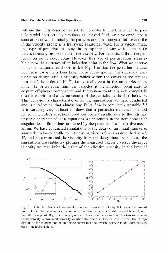
will use the units described in ref. 12. In order to check whether the par-ticle model does actually simulates an inviscid fluid, we have conducted asimulation in which initially the particles are in a triangular lattice and theinitial velocity profile is a transverse sinusoidal wave. For a viscous fluid,this type of perturbation decays in an exponential way with a time scalethat is inversely proportional to the viscosity. For an inviscid fluid the per-turbation would never decay. However, this type of perturbation is unsta-ble due to the existence of an inflection point in the flow. What we observein our simulations, as shown in left Fig. 1 is that the perturbation doesnot decay for quite a long time. To be more specific, the sinusoidal per-turbation decays with a viscosity which within the errors of the simula-tion is of the order of 10−10, i.e., virtually zero in the units selected asin ref. 12. After some time, the particles at the inflection point start toacquire off-planar components and the system eventually gets completelydisordered with a chaotic movement of the particles as the final behavior.This behavior is characteristic of all the simulations we have conductedand is a reflection that almost any Euler flow is completely unstable.(14)

It is certainly very difficult to show that a particular numerical methodfor solving Euler’s equations produces correct results, due to the intrinsicunstable character of these equations which reflects in the development ofsingularities in finite time, not cured by the presence of a dissipative mech-anism. We have conducted simulations of the decay of an initial transversesinusoidal velocity profile by introducing viscous forces as described in ref.12, and have measured the viscosity from the decay time. In this case, thesimulations are stable. By plotting the measured viscosity versus the inputviscosity we may infer the value of the effective viscosity in the limit of

Fig. 1. Left: Amplitude of an initial transverse sinusoidal velocity field as a function oftime. The amplitude remains constant until the flow becomes unstable around time 20, nearthe inflection point. Right: Viscosity η measured from the decay in time of a transverse sinu-soidal velocity versus input viscosity η0 when the model includes viscous forces. The extrap-olation of the straight line of unit slope shows that the inviscid particle model does actuallymodel an inviscid fluid.

140 Serrano et al.

zero input viscosity. The result is plotted in right Fig. 1 and it shows thatfor this smooth flow we have a well defined limit of zero input viscosityleading to zero measured viscosity.

The system described by Eqs. (6) and (7) reaches a dynamical equi-librium state apparently similar to the usual one in Molecular Dynamicssimulations. One would be tempted to describe this non-dissipative finalstate as a compressible homogeneous turbulence state corresponding to aninfinite Reynolds number (formal limit of zero viscosity). That this is notentirely the case can be quantified by measuring the kinetic energy spec-trum. While in the Kolmogorov theory it is given by a power law, in ourcase it is a flat spectrum corresponding to spatial white noise.

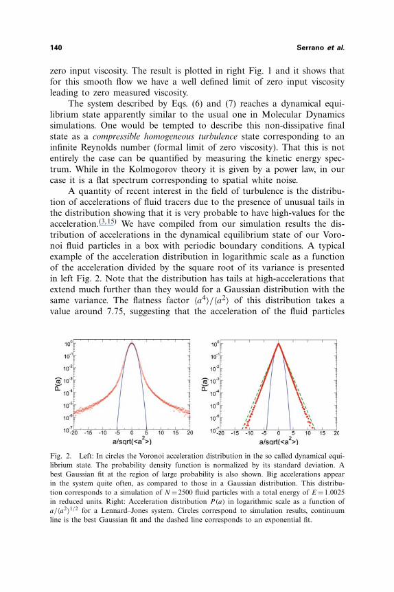
A quantity of recent interest in the field of turbulence is the distribu-tion of accelerations of fluid tracers due to the presence of unusual tails inthe distribution showing that it is very probable to have high-values for theacceleration.(3,15) We have compiled from our simulation results the dis-tribution of accelerations in the dynamical equilibrium state of our Voro-noi fluid particles in a box with periodic boundary conditions. A typicalexample of the acceleration distribution in logarithmic scale as a functionof the acceleration divided by the square root of its variance is presentedin left Fig. 2. Note that the distribution has tails at high-accelerations thatextend much further than they would for a Gaussian distribution with thesame variance. The flatness factor 〈a4〉/〈a2〉 of this distribution takes avalue around 7.75, suggesting that the acceleration of the fluid particles

Fig. 2. Left: In circles the Voronoi acceleration distribution in the so called dynamical equi-librium state. The probability density function is normalized by its standard deviation. Abest Gaussian fit at the region of large probability is also shown. Big accelerations appearin the system quite often, as compared to those in a Gaussian distribution. This distribu-tion corresponds to a simulation of N =2500 fluid particles with a total energy of E =1.0025in reduced units. Right: Acceleration distribution P(a) in logarithmic scale as a function ofa/〈a2〉1/2 for a Lennard–Jones system. Circles correspond to simulation results, continuumline is the best Gaussian fit and the dashed line corresponds to an exponential fit.

Fluid Particle Model for Euler Equations 141

is an intermittent variable (for Gaussian distributions the flatness factoris 3). The authors in ref. 3 make the observation that in fully developedturbulence the viscous damping term in Navier–Stokes equations is smallcompared to the pressure gradient term and, therefore, the accelerationis closely related to the pressure gradient. This may be the reason whyour discrete model still captures this intriguing feature of developed tur-bulence.

In order to see the relevance of the numerical result for the accel-erations in the Voronoi discrete model, we compute the accelerationdistributions in a Molecular Dynamics simulation for a purely repulsiveLennard–Jones type interaction (the WCA potential, see ref. 16). The ther-modynamic state of the system corresponds to a typical liquid conditiongiven by ρ = 0.844 for the fluid density and T = 0.71 for the temperature(in conventional reduced units in MD for Argon) while the number ofmolecules is NT =1000. The results for the probability distribution for theaccelerations P(a) as a function of the accelerations divided by the squareroot of its variance is shown in right Fig. 2. This distribution function hasan exponential form. The Molecular Dynamics distribution is very differ-ent from the one for the Voronoi fluid particle model.

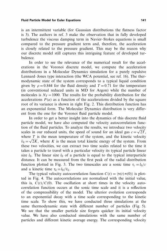
In order to get a better insight into the dynamics of this discrete fluidparticle model, we have also computed the velocity autocorrelation func-tion of the fluid particles. To analyze the results, we introduce two velocityscales in our reduced units, the speed of sound for an ideal gas c=√

2T ,where T is the mean temperature of the system, and the kinetic velocityvk =√

2K, where K is the mean total kinetic energy of the system. Fromthese two velocities, we can extract two time scales related to the time ittakes a particle to travel with a particular velocity its typical particle linearsize l0. The linear size l0 of a particle is equal to the typical interparticledistance. It can be measured from the first peak of the radial distributionfunction plotted in Fig. 3. The two timescales are a sonic time τc = l0/c

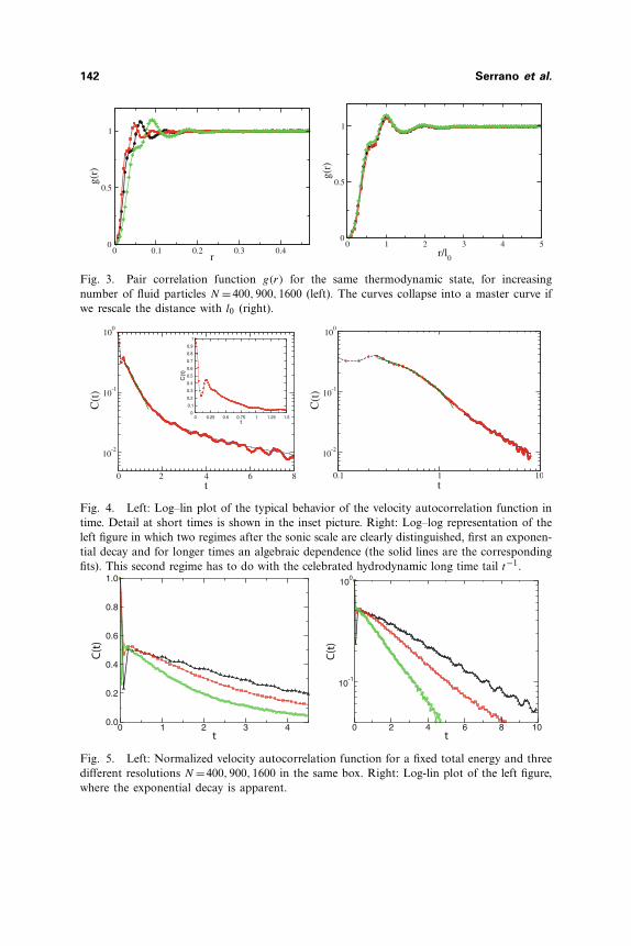
and a kinetic time τk = l0/vk.The typical velocity autocorrelation function C(t) = 〈v(t)·v(0)〉 is plot-

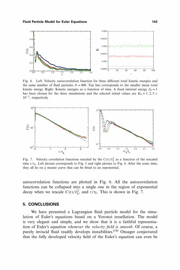
ted in Fig. 4. The autocorrelations are normalized with the initial value,this is, C(t)/C(0). The oscillation at short times in the velocity auto-correlation function occurs at the sonic time scale and it is a reflectionof the compressibility of the model. The ulterior evolution correspondsto an exponential decay with a time scale corresponding to the kinetictime scale. To show this, we have conducted three simulations at thesame thermodynamic state with different number of particles (Fig. 5).We see that the smaller particle size forgets quicker its initial velocityvalue. We have also conducted simulations with the same number ofparticles and different kinetic average energy. The corresponding velocity

142 Serrano et al.

0 0.1 0.2 0.3 0.4r

0

0.5

1

g(r)

0 1 2 3 4 5r/l

0

0

0.5

1

g(r)

Fig. 3. Pair correlation function g(r) for the same thermodynamic state, for increasingnumber of fluid particles N =400,900,1600 (left). The curves collapse into a master curve ifwe rescale the distance with l0 (right).

0 2 4 6 8t

0 0.25 0.5 0.75 1 1.25 1.5t

0

0.1

0.2

0.3

0.4

0.5

0.6

0.7

0.8

0.9

1

C(t

)

0.1 1 10t

10-2

10-1

100

100

C(t

)

10-2

10-1

C(t

)

Fig. 4. Left: Log–lin plot of the typical behavior of the velocity autocorrelation function intime. Detail at short times is shown in the inset picture. Right: Log–log representation of theleft figure in which two regimes after the sonic scale are clearly distinguished, first an exponen-tial decay and for longer times an algebraic dependence (the solid lines are the correspondingfits). This second regime has to do with the celebrated hydrodynamic long time tail t−1.

0 1 2 3 4t

0.0

0.2

0.4

0.6

0.8

1.0

C(t

)

0 2 4 6 8 10t

10-1

100

C(t

)

Fig. 5. Left: Normalized velocity autocorrelation function for a fixed total energy and threedifferent resolutions N =400,900,1600 in the same box. Right: Log-lin plot of the left figure,where the exponential decay is apparent.

Fluid Particle Model for Euler Equations 143

0.0 0.5 1.0 1.5 2.0 2.5 3.0t

0.0

0.2

0.4

0.6

0.8

1.0

C(t

)

0.0005

0.001

0.0015

0.002

0.0025

0.003

0 20 40 60 80 100

K

t

Fig. 6. Left: Velocity autocorrelation function for three different total kinetic energies andthe same number of fluid particles N = 400. Top line corresponds to the smaller mean totalkinetic energy. Right: Kinetic energies as a function of time. A fixed internal energy E0 = 1has been chosen for the three simulations and the selected initial values are K0 = 1,2,3 ×10−3, respectively.

0 1 2 3t /τΚ

10-2

10-1

100

C(t

)

0.0 0.5 1.0 1.5 2.0 2.5 3.0tv

K/l

0

10-1

100

C(t

)

Fig. 7. Velocity correlation functions rescaled by the C(t)/v2k as a function of the rescaled

time t/τk . Left picture corresponds to Fig. 5 and right picture to Fig. 6. After the sonic time,they all lie on a master curve that can be fitted to an exponential.

autocorrelation functions are plotted in Fig. 6. All the autocorrelationfunctions can be collapsed into a single one in the region of exponentialdecay when we rescale C(t)/v2

k, and t/τk. This is shown in Fig. 7.

5. CONCLUSIONS

We have presented a Lagrangian fluid particle model for the simu-lation of Euler’s equations based on a Voronoi tessellation. The modelis very elegant and simple, and we show that it is a faithful representa-tion of Euler’s equation whenever the velocity field is smooth. Of course, apurely inviscid fluid readily develops instabilities.(14) Onsager conjecturedthat the fully developed velocity field of the Euler’s equation can even be

144 Serrano et al.

non-differentiable.(17,18) In the fluid particle model this non-differentiabilitycan be assimilated to the chaotic and random motion of the final dynamicequilibrium state of the fluid particles. For a chaotic distribution of veloc-ities, one would conclude that it is not possible to define a derivative ofthe velocity field. Even though the model is purely reversible, the systemhas, at a coarse-grained level, an associated viscosity, in the same way as aLennard–Jones system (governed by Newtons’ reversible equations ofmotion) has a viscosity (which is a parameter that appears in the hydrody-namic equations). A given system may be described by reversible or irrevers-ible dynamic equations depending on the detail of the level of description.

The conclusion of the simulations is that the only relevant length inthe system is fixed by the fluid particle size (l0), and the exponential decayof the velocity autocorrelation function only depends on this scale and thekinetic velocity.

Despite of the fact that our model cannot be taken as the inviscid limitof the viscous Navier–Stokes equations, which is singular, we observe inthe model several statistical features that actually correspond to similar fea-tures observed in experiments on Lagrangian tracers in homogeneous fullydeveloped turbulence. In particular, we have observed that the fluid par-ticle velocity autocorrelation function shows an exponential decay beyondthe sonic scale. The characteristic decay time scales with the kinetic timescale. The higher the kinetic energy of the fluid particles (which is a mea-sure of the intensity of this “turbulence”), the fastest is the decay. As men-tioned in ref. 19, the exponential decay dictates a Lagrangian time scalethat appears as a time characteristic of the energy injection. This seems tobe also our case, where the kinetic time scale τk plays the role of the exper-imental Lagrangian time scale, related to the intensity of this “turbulence”.The acceleration distribution function reveals large tails that extend muchfurther than they would for a Gaussian distribution with the same variance.All these results agree with recent experimental results.(3,15) One possibleexplanation for this agreement is that in fully developed turbulence, the vis-cous damping term in Navier–Stokes equations is small compared to thepressure gradient term and therefore, the acceleration is closely related tothe pressure gradient, which is the only force in our model.

APPENDIX A. MATHEMATICAL PROPERTIES OF THE VORONOI

TESSELLATION

In this appendix, we summarize some mathematical properties of theVoronoi tessellation. Other interesting results and more detailed definitionsconcerning the Voronoi tessellation can be found in the appendix of ref.12. The Voronoi tessellation is a geometrical construction associated to

Fluid Particle Model for Euler Equations 145

a collection of N points in space, named cell centers or nodes, whichhave positions {R1, . . . ,RN }. The tessellation associates to every point theregion of space that it is closer to that point than to any other point of thecollection. This produces a partition of the space into a cellular structure.The common wall between two neighbor cells are, by definition, at equaldistance of the nodes of each cell and it is perpendicular to the vectorRij =Ri −Rj joining the nodes.

In this note, we will make extensive use of the smooth characteristicfunction χi(r) re-introduced by Flekkøy and Coveney,(20) and which areknown in a different context as Shephard functions. The smoothed char-acteristic function of the Voronoi cell i is defined as

χi(r)= �(|r −Ri |)∑j �(|r −Rj |) , (A.1)

where the function �(r) = exp{−r2/2σ 2} is a Gaussian of width σ . Thischaracteristic function satisfies the relations

∂χi(r)∂r

= 1σ 2

∑

j

χi(r)χj (r)(Ri −Rj ),∑

j

∂χi

∂Rj

=−∂χi

∂r. (A.2)

We can introduce the space average of a function f (r) over the Voronoicell i

[f ]i = 1Vi

∫drχi(r)f (r) Vi =

∫drχi(r), (A.3)

where Vi is the volume of the ith Voronoi cell.Consider now the cell average of the divergence of an arbitrary vector fieldA(r), this is

[∇·A]i = 1Vi

∫drχi(r)∇·A(r)

= 1Vi

∫

∂V

dS·A(r)χi(r)− 1Vi

∫drA(r)·∇χi(r), (A.4)

where we have made use of Gauss’ theorem. The first surface integral overthe boundary of the full domain will vanish if the cell i does not cross thisboundary (in which case the characteristic function of cell i vanishes forall points of the boundary).

By using the first relation in Eq. (A.2) we have

146 Serrano et al.

[∇·A]i = − 1Vi

∫drA(r)·∇χi(r)

= 1Vi

∑

j

Rij

1σ 2

∫drA(r)χi(r)χj (r). (A.5)

First, let us assume that the vector field is just constant. Its divergence willbe simply zero. This implies the following identity

0=− 1Vi

∑

j

Rij

Aij

Rij

·A, (A.6)

where we have introduced

Aij =Rij

1σ 2

∫drχi(r)χj (r). (A.7)

This quantity Aij becomes in the limit σ → 0 the area of the faceof contact between cells i, j . Equation (A.6) becomes then

∑j Aij eij = 0,

where eij is the unit vector normal to the face i, j . Therefore, Aij eij isthe “surface vector” of face i, j . In words,

∑j Aij eij = 0 states that for

any given Voronoi cell not on the boundary of the system, the sum of the“surface vectors” over the cell vanish.

Second, let us assume that the vector field A(r) depends linearly onthe positions, this is, A(r) = �·r, where � is a constant matrix. Substitu-tion in Eq. (A.5) leads to

tr� = − 1Vi

∑

j

Rij ·�· 1σ 2

∫drχi(r)χj (r)r

= − 1Vi

∑

j

Aij eij Cij :�, (A.8)

where the double dot means double contraction. The vector Cij is definedthrough this very equation and is, in the limit σ → 0 the position of thecenter of mass of the face i, j . For arbitrary matrices � (and, in particu-lar, for those matrices � with only one single entry different from zero),Eq. (A.8) holds if and only if

− 1Vi

∑

j

Aij eij Cij =1, (A.9)

where 1 is the identity matrix.

Fluid Particle Model for Euler Equations 147

ACKNOWLEDGMENTS

This work has been supported by the Spanish Ministerio de Educaciony Ciencia with the Grant No FIS2004-01934. We thank Mariano Revengafor his visualization program PUNTO.

REFERENCES

1. U. Frisch, Turbulence (Cambridge University Press, 1995).2. G. Falkovich, K. Gawedzki, and M. Vergassola, Particles and fields in fluid turbulence,

Rev. Mod. Phys. 73:913 (2001).3. A. L. Porta, G. A. Voth, A. M. Crawford, J. Alexander, and E. Bodenshatz, Fluid parti-

cle accelerations in fully developed turbulence, Nature 409:1017 (2001).4. L. D. Landau and E. M. Lifshitz, Fluid Mechanics (Pergamon Press, 1959).5. J. J. Monaghan, Sph compressible turbulence, Mon. Not. R. Astron. Soc. 335(3):843–852

(2002).6. J. J. Monaghan and D. Price, Variational principles for relativistic smoothed particle

hydrodynamics, Mon. Not. R. Astron. Soc. 328(3):381–392 (2001).7. H. Lamb, Hydrodynamics, 6th ed. (Cambridge University Press, 1932).8. G. A. Kuz’min, Ideal incompressible hydrodynamics in terms of the vortex momentum

density, Phys. Let. 96A:88–90 (1983).9. V. I. Osledets, On a new way of writing the Navier Stokes equation: The Hamiltonian

formalism, Russ. Math. Surveys 44:210–211 (1989).10. P. Espanol, M. Serrano, and H. C. Ottinger, Thermodynamically admissible form for dis-

crete hydrodynamics, Phys. Rev. Lett. 83:4542 (1999).11. P. Espanol and M. Revenga, Smoothed dissipative particle dynamics, Phys. Rev. E

67:026705 (2003).12. M. Serrano and P. Espanol, Thermodynamically consistent mesoscopic fluid particle

model, Phys. Rev. E 64:046115 (2001).13. I. Wenneker, A. Segal, and P. Wesseling, Computation of compressible flows on unstruc-

tured staggered grids, (2000) in ECCOMAS 2000 (Barcelona), E. Onate, G. Bugeda andB. Suarez.

14. S. Friedlander and A. Lipton-Lifschitz, Localized instabilities in fluids, Handbook ofMathematical Fluid Dynamics, 2003 – math.uic.edu.

15. N. Mordant, J. Delour, E. Leveque, A. Arneodo, and J. F. Pinton, Long time corre-lations in Lagrangian dynamics: A key to intermittency in turbulence, Phys. Rev. Lett.89:254501–1 (2002).

16. J. D. Weeks, D. Chandler, and H. C. Andersen, The Role of Repulsive Forces in Deter-mining the Equilibrium of Simple Liquids, J. Chem. Phys. 54:5237 (1971).

17. L. Onsager, Statistical hydrodynamics, Nuovo Cimento, VI:280–287 (1949).18. G. L. Eyink, Energy dissipation without viscosity in ideal hydromechanics, i. Fourier

analysis and local energy transfer, Physica D 78:222–240 (1994).19. N. Mordant, P. Metz, O. Michel, and J.-F. Pinton, Measurement of Lagrangian velocity

in fully developed turbulence, Phys. Rev. Lett. 87:214501–1 (2001).20. E. G. Flekkøy and P. V. Coveney, From molecular to dissipative particle dynamics, Phys.

Rev. Lett. 83:1775 (1999).