A Two-Factor Uncertainty Model to Determine theOptimal Contractual Penalty for a

Build-Own-Transfer Project

João Adelino Ribeiro∗†, Paulo Jorge Pereira

‡and Elísio Brandão

§

October 17, 2013

Abstract

Public-Private Partnerships (PPP) became one of the most common types of public procurement arrangementsand Build-Own-Transfer (BOT) projects, awarded through adequate bidding competitions, have been increasinglypromoted by governments. The theoretical model herein proposed is based on a contractual framework wherethe government grants leeway to the private entity regarding the timing for project implementation. However, thegovernment is aware that delaying the beginning of operations will lead to the emergence of social costs, i.e., thecosts that result from the corresponding loss of social welfare. This fact should motivate the government to includea contractual penalty in case the private firm does not implement the project immediately. The government alsorecognizes that the private entity is more efficient in constructing the project facility. The model’s outcome is theoptimal value for the legal penalty the government should include in the contract form. A two-factor uncertaintyapproach is adopted and Adkins and Paxson (2011) quasi-analytical solution is applied since homogeneity of degreeone can not be invoked in all of the model’s boundary conditions. Sensitivity analysis reveals that variations inthe correlation coefficients have a strong impact on the optimal contractual penalty and also that there is a levelfor the comparative efficiency factor above which there is no need to impose a contractual penalty, for a givenlevel of social costs. Finally, the effects of including a non-optimal penalty value in the contract form, whichderives from overestimating or underestimating the selected bidder’s real comparative efficiency are examined,using a numerical example. Results demonstrate that overestimating (underestimating) the selected bidder’s realcomparative efficiency leads to the inclusion of a below-optimal (above-optimal) value for the legal penalty in thecontract and produces effects that the government would prefer to prevent.

JEL Classification Codes: G31; D81.

Keywords: real options; two-factor uncertainty models; public-private partnerships; optimal contractual penalty.

∗João Adelino Ribeiro acknowledges the financial support provided by FCT (Grant nº SFRH/BD/71447/2010)†PhD Student in Finance, Faculty of Economics, University of Porto, Portugal; email: 090427012@fep.up.pt‡Assistant Professor at Faculty of Economics, University of Porto, Portugal; email: pjpereira@fep.up.pt§Full Professor at Faculty of Economics, University of Porto, Portugal; email: ebrandao@fep.up.pt

1

Part I

Introduction

1 Review of the Literature

1.1 Build-Operate-Transfer (BOT) Projects in the Context of Bidding Competi-

tions

Public-Private Partnerships (PPP) became one of the most important types of public pro-curement arrangements and its importance has been growing considerably in the lastdecades (Kwak et al. (2009); Alonso-Conde et al. (2007); Algarni et al. (2007); Hoand Liu (2002)). PPP is usually defined as a long-term development and service con-tract between the government and a private partner (Maskin and Tirole (2008)). Thistype of contract may assume different forms and the Build-Own-Transfer (BOT) modelis widely adopted (Liu and Cheah (2009); Ho and Liu (2002)). BOT is the terminologyfor a project structure that uses private investment to undertake the infrastructure devel-opment, and which has been historically ensured by the public sector.1 In fact, the privatesector has been playing an increasingly crucial role in the financing and provision of ser-vices that were traditionally in the domain of the public sector. One of the key reasons isthat governments are unable to cope with the ever-increasing demands on their budgets.Most infrastructure expenditures in developing - and also in developed countries - havebeen funded directly from fiscal budgets but several factors such as the macroeconomicinstability and growing investment needs have shown that public finance is volatile and,in many of those countries, rarely meet the infrastructure expenditure requirements in atimely and adequate manner (Ferreira and Khatami (1996)).

In BOT projects, a private entity is given a concession to build an infrastructure andoperate a facility which, as we just mentioned, would traditionally be built and operated bythe government or a public agent (Shen and Wu (2005)). At the end of the predeterminedconcession period (a period that tends to be long), the private party returns the ownershipof the infrastructure to the government or the public entity (Shen et al. (2002)).2

1The acronym BOT is often used interchangeably with BOOT (build-own-operate-transfer). Other ar-rangements include BOO (build-own-operate), a type of contractual scheme where the private party doesnot carry the obligation of transferring the ownership in any date, meaning that the private partner mayoperate the facility forever, as in the case of a typical private investment project.

2Given that BOT/BOOT schemes are designed and implemented as Public-Private Partnership contrac-tual arrangements, we will consider, for the purpose of the present work, BOT and PPP designations asbeing synonyms.

2

BOT infrastructure projects also differ significantly from the construction projects wehave considered in Chapters II and III in how they are implemented during the pre-construction phase. In the case of construction projects, the public party is responsible forproject planning, property acquisition and, more importantly, project funding. For BOTprojects, the concessionaire (private party) is usually required to undertake these projectdevelopment tasks (Huang and Chou (2006)). This contractual arrangement provides amechanism for using private finance, hence allowing the public sector to construct moreinfrastructure services without the use of additional public funds (Shen and Wu (2005)) .

BOT projects are awarded through an appropriate bidding competition process, where anumber of private entities compete to win the contract. As with the other type of con-struction projects - and all other things being equal - the contract will be awarded to thebidder that presented the most competitive bid, which, in the case of BOT projects, meansthe bidder that offered the highest price.3 The price is the amount to be paid to the gov-ernment to own the right to operate the facility once the obligation of constructing theinfrastructure is fulfilled. Hence, the selected bidder will be invited to sign the contractand - if the contract is actually signed - he or she will have to invest in constructing thefacility and run the subsequent operations, once the construction phase is completed.

1.2 The Application of the Real Options Approach to BOT Projects

A considerable number of research pieces can be found where the real options approach isapplied to address different questions concerning BOT projects. Some of the most impor-tant issues concern project valuation, how several risk types should be shared between theparties, the role of incentives and subsidies given by the government or the public agentand also the well-known mechanism of the Minimum Revenue Guarantee (MRG). By ad-dressing these topics using the real options approach, researchers acknowledge that thismethodology seems to be the most adequate, since a number of real options are availableto both parties throughout the life of the project. Thus, flexibility is a feature that can befrequently found on existing contracts and the levels of uncertainty surrounding this typeof projects tend to be high. By recognizing the irreversibility of this type of investmentsand also the uncertainty and flexibility that characterizes BOT projects, some researchersadopt the real options approach to evaluate options embedded in current contract types,while others use it to sustain and propose different forms of shaping contracts betweenthe parties, namely by suggesting that incorporating more flexibility in the contractual

3In construction projects - and all other things being equal - the selected bidder is the one that presentedthe lowest bid. For obvious reasons, in a BOT project competitive bid, is the other way around: all elseequal, the selected bidder will be the one that offered the highest price.

3

relationship may lead to more economic efficiency at different levels. Various researchpieces can be found focusing on one or more of the above research topics. For exam-ple, Huang and Chou (2006) valued the MRG and the option to abandon the project bythe private firm, and Brandao and Saraiva (2008) also developed a model for infrastruc-ture projects based on the consideration of a Minimum Demand Guarantee. Cheah andLiu (2006) addressed the valuation of demand and revenue guarantees, applying MonteCarlo simulation, and Chiara et al. (2007) also applied the same technique to evaluate aMRG, which is only redeemable at specific moments in time. Alonso-Conde et al. (2007)addressed the existing contractual conditions in PPP which guarantee a minimum prof-itability to the private firm. Shan et al. (2010) proposed collar options (a call option anda put option combined) to better manage revenue risks. Huang and Pi (2009) applied asequential compound option approach for valuing multi-stage BOT projects, in the pres-ence of dedicated assets. Caselli et al. (2009) valued the indemnification provision thatensures a final compensation to the private partner, in the event the government termi-nates a BOT contract. Armada et al. (2012) showed how the net cost of incentives, whichmay be given by the government to induce the immediate investment, should equal thevalue of the option to defer the beginning of operations by the private firm. Pereira et al.(2006) applied a two-factor uncertainty model aiming to reach the optimal timing for theconstruction of an international airport, where the cash-flows to be generated were dis-aggregated into the number of passengers and the net cash-flow “per passenger”. Theirmodel is thus based on the existence of two stochastic variables, but they considered theinvestment costs constant.

1.3 Two-Factor Uncertainty Models in the Real Options Literature

All of the above research pieces do not consider the two key-value drivers of a BOTproject - the construction costs and cash-flows to be generated by operations - as stochasticvariables. To the best of our knowledge, the only research piece based on a two-factoruncertainty model, in the context of BOT projects, where the stochastic variables arethe present value of the cash-flows and the construction costs is the paper by Ho andLiu (2002). In fact, these researchers considered the construction costs and the presentvalue of cash-flows as being both stochastic variables, behaving according to GeometricBrownian Motions. However, their model is designed in discrete time, more specificallyapplying the well-known binomial model, with the purpose of valuing a debt guaranteegiven by the government, and also accounting for the risk of bankruptcy. The model wepropose and describe in Section 4.3 is a two-factor uncertainty model in continuous time,where both construction costs and cash-flows follow geometric Brownian motions that

4

are possibly correlated and, to the best of our knowledge, is the first model apllying atwo-factor uncertainty approach in continuous-time, in the context of BOT projects.

In fact, the consideration of both key-value drivers of BOT projects as stochastic vari-ables is not a common feature in existing models. However, we should stress that, inrecent years, two-factor uncertainty models have been increasingly adopted to addressother research topics in the field of real options, such as the research pices carried out byArmada et al. (2013), Adkins and Paxson (2011) and Paxson and Pinto (2005).

The traditional real options model on the optimal timing to invest in a project with ir-reversible costs and generating perpetual cash-flows was first developed by McDonaldand Siegel (1986), where both the value of expected cash-flows and the investment costsare considered to behave stochastically. This model is carefully explained in Dixit andPindyck (1994). These authors describe the model but held the investment costs con-stant in a first stage. Later in their text book, Dixit and Pindyck (1994) address thebi-dimensionality issue - thus recognizing the stochastic nature of the investment costs- and present McDonald and Siegel (1986) solution, which consists of reducing the twostochastic variables to just one, by merely substituting the cash-flows and investment costsby a single variable (ratio) that equals the cash-flows divided by the investment costs. Mc-Donald and Siegel (1986) model is also described in Trigeorgis (1996). Both Trigeorgis(1996) and Dixit and Pindyck (1994) stated that it is optimal to invest when the ratio be-tween the expected cash-flows and the investment costs reaches a given boundary: theso-called “free boundary”, separating the waiting region from the investing region. Thismethod may be very useful to address some BOT projects related issues but, unfortu-nately, we cannot apply it to all situations in the context of the present work, since wecan not invoke homogeneity of degree one in all the boundary conditions, unlike whathappens in McDonald and Siegel (1986) model.4

The model we suggest is based on the recognition of uncertainty in both the facility con-struction costs and in the value of the cash-flows that will be generated by operating theproject facility, which means that a two-factor uncertainty framework will be adopted,with both variables following geometric Brownian motions that are possibly correlated.In the next Section, we detail the proposed framework, where the government grants lee-way to the selected firm regarding the timing for project implementation, which meansthat the private firm may implement the project when he or she decides that is optimalto do so. However, we propose that a contractual penalty should be established in theevent the private firm does not implement the project immediately. The theoretical model

4Since their boundary conditions do not infringe homogeneity of degree one, the model proposed bythese researchers respect the condition which states that the sum of the roots of the quadratic equationequals 1. A closed-form solution is thus reached.

5

aims to determine the optimal level for this contractual penalty. The determination of theoptimal level for this penalty will consider the argument that the selected firm is moreefficient than the government in executing the project facility, and also that the govern-ment recognizes the existence of social costs, i.e., the costs that correspond to the lossof social welfare, which emerge if the project is not implemented immediately. If weconsider that both entities are equally efficient, then the optimal penalty would be the onethat would induce the selected firm to invest in the same moment the government would,if the government decided to undertake the project. However, we will demonstrate that -by assuming that the private firm is more efficient than the government in executing theproject facility - the optimal contractual penalty is the one that makes the private firminvest when his or her value for the cash-flows trigger equals the value of the governmentcash-flows trigger, for a given project dimension and assuming a specific level of com-parative efficiency. In fact, by considering that the private firm is more efficient, then onewould expect the private firm to invest sooner than the government: he or she will attainhis or her construction costs trigger sooner than the government will attain its construc-tion costs trigger. By attaining the construction costs trigger sooner than the government,and since the optimal contractual penalty is the one that makes both entities have the sametrigger for the cash-flows, consequently one expects the private firm to invest sooner thanthe government would, if the government decided to conduct the project. In fact, by in-troducing the higher efficiency of the private firm in the model, we can not define theoptimal penalty as being the one that makes both entities have the same combination oftriggers, i.e., expectedly,to invest in same moment of time. Rather, in the presence ofthe private firm’s higher efficiency, the optimal penalty should be defined as the one thatmoves the private firm cash-flows trigger downwards in order to meet the governmentcash-flows trigger, for a given project dimension and considering the estimated value forthe comparative efficiency factor.

2 Proposed Framework

2.1 Flexibility May Imply a Cost. The Contractual Penalty

We define a conceptual framework where a BOT project may be undertaken by the gov-ernment or then awarded to a private firm through an appropriate competitive bid process,maybe because the government recognizes that is less efficient than the private firm inexecuting the project. We suggest that the project may be initiated whenever the selectedbidder decides it is optimal to do so, meaning that no contractual obligation for imme-diate initiation of activities is imposed by the government. This assumption regarding

6

the absence of any contractual obligation regarding the immediate implementation of theproject has also been adopted by Armada et al. (2012), and plays a crucial role in the con-text of the research questions they have addressed. The motivation of their research worklies on the argument that the private firm will start investing later than the governmentwould like him or her to, since the option to defer the project implementation does havevalue. Bearing this in mind, they studied how certain subsidies and guarantees, grantedto the private firm, can be optimally arranged with the purpose of inducing the immediateimplementation of the project. We build the present framework on the same assumptionbut argue that, under certain conditions, a legal penalty should be enforced in the eventthe construction of the facility does not start immediately. Thus, and even though weacknowledge that the private firm may manage the project implementation as far as itsinitiation/completion is concerned, we suggest that a penalty should be enforced in thecase the infrastructure is not ready and operations do not start immediately. This meansthat the private firm is aware of the fact that delaying the project implementation maygrant him some benefits (there is value to waiting for more information) but is also awarethat deferring the beginning of the project may entail a cost. Thus, the private firm hasflexibility regarding the moment to start running operations but this flexibility may implya cost. We propose that, under certain conditions, which we will discuss later on in thispaper, this cost should be considered in the contract form, assuming the form of a legalpenalty.

2.2 The Importance of the Efficiency Factor

We have to acknowledge that governments are, in most cases, less efficient than pri-vate firms in conducting BOT projects. This argument is common in the literature andis frequently invoked as being one of the reasons why governments actually grant theprojects to the private sector (see, for example, Brandao and Saraiva (2008); Zhang andKumaraswamy (2001)). Being so, one should expect the private firm to invest earlier dueto its greater efficiency. To be more efficient means being able to construct the facilityinvesting less money than the government would. Hence, if the expected constructionscosts of the private firm are lower than the construction costs estimated by the govern-ment, then - all else equal - the private firm will attain the critical value for the cash-flowsto be generated by operations that triggers the investment sooner than the government.This is the same as saying that one expects the private firm to invest in an earlier momentof time than the government would.

Hence, by considering that the private firm is more efficient than the government, we areassuming that the private firm will have a lower trigger for his or her construction costs

7

than if both entities were considered to be equally efficient because, if both entities wereequally efficient, then they would have the same construction costs trigger. This greaterefficiency leads us to conclude that the efficiency factor places the firm construction coststrigger before the government construction costs trigger, “vis-a-vis” with the scenariowhere both entities are equally efficient. Furthermore, the greater the level of comparativeefficiency, the lower the private firm construction costs trigger will be or, which is thesame, the further backwards its construction costs trigger will be shifted, again whencompared with the “equally efficient scenario”.

Considering the private firm’s greater efficiency, the government’s purpose is accom-plished if the private firm invests when his or her cash-flows trigger equals the governmentcash-flows trigger. We would like to underline this argument: by enforcing an optimal le-gal penalty, the government’s purpose is to induce the private firm to invest when he orshe has a cash-flows trigger whose value equals the value of the government cash-flowstrigger. This implies that, without the enforcement of the legal penalty, the private firmcash-flows trigger will be higher than the government cash-flows trigger. We will showthat this inequality holds since the government cash-flows trigger is affected by anothercrucial element that the model encompasses. We designate this element as “social costs”.

2.3 The Importance of Social Costs

The traditional concept of “social cost” was addressed by Coase (1960) and is based on theconcept of “externality”, in the sense that, by producing a certain good, a harmful effect iscaused to the society, rather than the owners of the firm responsible for the production ofthat good or its customers. It is a cost which society must ultimately bear. This naturallyentails that a loss of welfare occurs to the population due to the emergence of this exter-nality. Hence, this loss of welfare is not a direct consequence of the fact that a firm is notproducing a good or providing a service to its customers. Rather, social cost is exactly de-fined as being the cost borne by the population because a certain good is being producedand such fact causes an undesirable effect to the population. Notwithstanding, we reasonthat, when a government or a government agency decides to implement a project, its goalis to provide a service to the population. The government decision of, say, implementinga High-Speed Rail service is based on the conviction that the project will generate a socialbenefit, as stated by Rus and Nombela (2007). Hence, the government believes that socialbenefits occur as soon as the project is implemented and operations start because socialwelfare will emerge once the project is completed. Bearing this important argument inmind, we state that, on the contrary, if the project is not implemented immediately, a lossof welfare occurs and this is the same as stating that the social benefits emerging from the

8

immediate project implementation are postponed until the project is actually completedand the subsequent activities start. We thus argue that the lack of social benefits fromthe moment the project should have been ready and the moment the project is, in fact,ready and operations begin can be legitimately defined as “social costs”.5 Social costsare, therefore, directly related with the loss of welfare that occurs if the project is notimplemented immediately. Again, these costs correspond to the loss of social welfare oc-curred from the time the project should have been ready to start operating and providingservices to its users and the moment operations actually begin and the users needs startbeing satisfied. Being so, our model considers the existence of social costs in the case theproject is not implemented immediately.

Social costs, as we define them, are rarely negligible. Large-scale investments are un-dertaken because governments believe that public needs must be satisfied and such needswill only be satisfied once the project is completed and subsequent operations begin. Thelevel of the social costs may be high for some projects, moderate for other projects oreven low in fewer cases.6 We will consider that social costs are estimated by the govern-ment as being a percentage of the expected cash-flows to be generated by operations. Byestimating an expected level of social costs, the government is setting its own cash-flowstrigger or, which is the same, is defining the precise moment where the project would beinitiated if the government decided to undertake the project. Nevertheless, when defin-ing the moment where the project would be implemented, the government behaves asa rational agent, in the sense that also considers the benefits of waiting and invest in alater date (meaning that the government recognizes that there is value to waiting, regard-less of which entity will conduct the project) and compares such benefits with the factthat, the later the project will be implemented, the higher the value of social costs willbe. Thus, when the government sets its own cash-flows trigger, by defining the level ofsocial costs considered to be tolerable, the government takes into account the fact thatwaiting for better information does have value. The government cash-flows trigger willthus result from a trade-off between the benefits of waiting and, hence, not invest imme-diately and the level of social costs to be borne by the population, if the project is notpromptly initiated. We argue that, when establishing the level of social costs consideredto be acceptable, the government also takes into account the benefits that derive from de-

5We would like to underline the argument that our definition of “social costs” differs from the definitionof “social cost”, as in Coase (1960). This means that we are not using this concept in the context of thepresent work since we are not considering the importance of the emergence of social cost(s), which result(s)from some kind of externality.

6Currently in Portugal, there is a stream of opinion that questions the benefits of some large-scale in-vestments undertaken in the recent past, especially the construction of highways linking the cities of Lisbonand Porto, which are considered by many to be redundant. In such cases and following this line of thought,delaying the initiation of large-scale investments whose social benefits are perceived as being very low willentail a very low level of social costs.

9

laying the project implementation. Consequently, the greater the level of social costs thegovernment considers to be acceptable, the sooner the government would invest. On thecontrary, for lower levels of acceptable social costs, the government will invest later. Wewill numerically demonstrate the existence of this relationship in Part II.

2.4 The Definition of Optimal Contractual Penalty

Social costs do play a fundamental role in establishing the optimal level for the contractualpenalty to be enforced in the event the project is not initiated immediately. The greater thelevel of social costs the sooner the government would invest and the higher the optimalpenalty needs to be, with the purpose of moving the cash-flows trigger downwards to meetthe government cash-flows trigger, which is now placed more below. On the contrary,the lower the level of social costs the smaller the optimal penalty needs to be (since thegovernment cash-flows trigger is now placed more above) and, if the level of social costsis zero, then a legal penalty is not needed, which is the same as saying that the optimallevel is zero. Hence, we define the optimal value for the contractual penalty as the onethat moves the private firm cash-flows trigger downwards with the purpose of meetingthe government cash-flows trigger, assuming that the private firm cash-flows trigger ishigher than the government cash-flows trigger. Bearing this definition in mind, we haveto conclude that any value for the contractual penalty that does not move the privatefirm cash-flows trigger downwards in order to perfectly meet the government cash-flowstrigger will never be optimal. In Part II, we will discuss the effects, to the government,that derive from including a non-optimal level for the legal penalty in the contract form.

The remainder of the present paper unfolds as follows. In Part II, the model is describedand both the government decision to invest and the government expectation about theprivate firm decision to invest are presented. The optimal level for the contractual penalty“per unit” of cost is then reached, considering the effect of the estimated efficiency factorand also the effect caused by the level of social costs. We proceed to perform a sensitivityanalysis, aiming to assess the impact of variations in various parameters of the model onthe optimal contractual penalty. More specifically, we measure how the optimal value forthe contractual penalty is affected by (i) changes in the level of social costs; (ii) changesin the efficiency factor; (iii) variations in both the level of social costs and the level of thecomparative efficiency factor; (iv) variations in the correlation coefficients; (vi) variationsin the standard deviations of both variables. Also, we derive an analytical solution to thelevel of the efficiency factor above which the inclusion of legal penalty is not justified, fora given level of social costs. Still in Part II, we examine the effects, to the government, ofincluding a non-optimal value for the legal penalty in the contract from, as a direct result

10

of overestimating or underestimating the comparative efficiency factor. Finally, in PartIII, conclusions are given.

Part II

The Model

2.5 Assumptions

We assume that (i) the government has the necessary know-how to determine fair esti-mates about the construction costs and the cash-flows to be generated through operatingthe facility, as if the project was conducted by the government; (ii) the standard devia-tions of the facility construction costs and of the future cash-flows are the same for boththe government and the private firm, since variations in the value of the project inputs andthe project outputs are both observable in the markets; (iii) the rate of return-shortfalls(i.e., the “convenience yields”) are also the same for both entities; (iv) the governmentrecognizes that is less efficient in constructing the project facility than the private firm;(v) the government is capable of determining a fair estimate for the private firm’s higherlevel of efficiency; (vi) the construction of the facility is assumed to be instantaneous;7

(vii) the project, once implemented, will generate perpetual cash-flows;8 (viii) the gov-ernment incurs in social costs if the project is not completed and operations do not startimmediately; (ix) social costs are assumed to be a percentage of the cash-flows to be gen-erated by operations; (x) the project dimension is given by the government’s expectedconstruction costs.

2.6 Model Description

2.6.1 Introduction

We depart from considering that the various sources of uncertainty underlying a BOTproject may be reduced to two aggregated sources: the uncertainty regarding the value

7By assuming that the construction of the facility is instantaneous, we are implicitly considering thatno flexibility is present throughout the construction stage. Therefore, we exclude the existence of optionsduring this stage. Since flexibility is not considered, we are only concerned with the fact that constructioncosts are uncertain.

8We assume that the concession period is sufficiently long for the investment opportunity to be consid-ered equivalent to a perpetual call option. This is a common assumption in the literature. See, for example,Armada et al. (2012).

11

of the future cash-flows to be generated by operations, V , and the facility constructioncosts, K. In specific situations, we will follow Adkins and Paxson (2011) approach, alsobased on a two-factor uncertainty model, and consisting of a set of simultaneous equa-tions. These authors developed a quasi-analytical solution, whereby a boundary betweenthe continuance and the renewal regions (i.e., the boundary separating the regions wherevalues for both variables justify an incumbent asset to continue operating or to be renewedand, thus, substituted by a new one by paying a fixed cost) is determined, since they areunable to invoke homogeneity of degree one in their model. We will show that some of thequestions we propose to answer can not be addressed by invoking homogeneity of degreeone, hence leading us to follow Adkins and Paxson (2011) approach. By considering thata trade-off exists between the two stochastic variables and also that only when both trig-gers are simultaneously attained investment is triggered, Adkins and Paxson (2011) statethat a countless set of pairs for such triggers do exist, i.e., there is an infinite combinationof possible threshold values for both variables. In our model, it is possible to envisagea countless pair of threshold values for the stochastic variables, V ∗ and K∗ and also thatthis countless set of pairs defines the discriminatory boundary that separates the waitingregion from the investing region. A variation in one of the variables leads to a variation ofthe same sign in the other for the investment to be triggered. In fact, lower constructioncosts will necessarily lead to a lower value of cash-flows to trigger the investment and,similarly, a higher value of construction costs will lead to a higher cash-flows value whichtriggers the investment. As Dixit and Pindyck (1994) point out, the value of the option toinvest depends on both variables, which means that the option will be exercised when V

becomes sufficiently high for a given K or K becomes sufficiently low for a given V . Onthe contrary, if V is not sufficiently large for a given K or K is too low for a given V, thenone would expect the option to be held. Hence, we are aware that is possible to define anoptimal boundary composed by a set of pairs for V ∗ and K∗ that discriminates the waitingregion from the investing region. We will denote this set of trigger values as {V ∗,K∗}.

We proceed to present the base case parameter values and derive the government decisionto invest, bearing in mind that social costs are present and considered to be a percentage ofthe cash-flows to be generated by operations. This implies that the government recognizesthe fact that, if the project is not implemented immediately, a loss of social welfare occursuntil the project is completed and operations actually start. We then derive the governmentexpectation about the private firm investment decision, assuming the private firm is moreefficient than the government in executing the project facility. Finally, we determine theoptimal value for the contractual penalty “per unit” of cost, and consider three differentproject dimensions, for illustrative purposes.

For both cases, i.e., the government decision to invest and the expectation the government

12

has about the private firm’s decision to invest, the two stochastic variables (the value ofthe cash-flows to be generated by operations, V , and the facility construction costs, K)follow geometric Brownian motions that are possibly correlated. Let i ∈ {G,P}. Hence:

dVi = αViVidt +σViVidzVi (1)

dKi = αKiKidt +σKiKidzKi (2)

E(dzVidzKi) = ρidt (3)

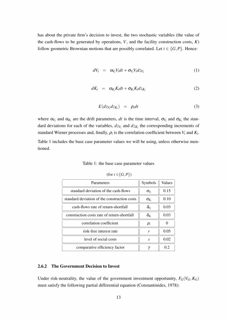
where αVi and αKi are the drift parameters, dt is the time interval, σVi and σKi the stan-dard deviations for each of the variables, dzVi and dzKi the corresponding increments ofstandard Wiener processes and, finally, ρi is the correlation coefficient between Vi and Ki.

Table 1 includes the base case parameter values we will be using, unless otherwise men-tioned.

Table 1: the base case parameter values

(for i ∈{G,P})

Parameters Symbols Values

standard deviation of the cash-flows σVi 0.15

standard deviation of the construction costs σKi 0.10

cash-flows rate of return-shortfall δVi 0.03

construction costs rate of return-shortfall δKi 0.03

correlation coefficient ρi 0

risk-free interest rate r 0.05

level of social costs s 0.02

comparative efficiency factor γ 0.2

2.6.2 The Government Decision to Invest

Under risk-neutrality, the value of the government investment opportunity, FG(VG,KG)

must satisfy the following partial differential equation (Constantinides, 1978):

13

12

σ2VG

V 2G

∂ 2FG

∂V 2G

+12

σ2KG

K2G

∂ 2FG

∂K2G+ρσVGσKGVGKG

∂ 2FG

∂VG∂KG+

(r−δVG)VG∂FG

∂VG+(r−δKG)

∂FG

∂KG− rFG− sVG =0 (4)

where r is the risk-free interest rate, sVG denotes the value of social costs as a percentageof the cash-flows to be generated by the project operations, δVG and δKG are the rates ofreturn-shortfall for VG and KG, respectively, which are given by the following equations:

δVG = r−αVG (5)

δKG = r−αKG (6)

The following general solution satisfies the partial differential equation (4):

FG(VG,KG) = A1V β+

G Kη+

G +A2V β+

G Kη−

G +A3V β−

G Kη+

G +A4V β−

G Kη−

G −s

δVG

VG (7)

where A1, A2, A3 and A4 are constants that need to be determined. β+, β−, η+ and η−

are the four roots of an elliptical equation, which is the two-factor counterpart of the one-factor stochastic model quadratic equation presented in Dixit and Pindyck (1994). Theelliptical equation is:

Q(β ,η) =12

σVGβ (β −1)+12

σ2KG

η(η−1)+

ρGσVGσKGβη +(r−δVG)β +(r−δKG)η− r = 0 (8)

The function Q(β ,η) = 0 defines an ellipse.9 Equation (8) has four quadrants, to whichof them corresponds a pair of the four roots just mentioned, i.e., the four points wherethe elliptic function meets the axes. If we now consider the absorbing barriers FG(0,0),FG(0,KG), thus A3 = A4 = 0, since the option to invest is worthless if the present value offuture cash-flows is zero. Likewise, for FG(VG,KG), and as KG becomes infinitely largefor any value of VG, then the option is also worthless. To respect this condition, we needto set constant A1 = 0, leaving only constant A2 6= 0. Thus, in our case, the quadrant

9Please refer to Adkins and Paxson (2011) for more details.

14

of interest is the second one, corresponding to the pair of roots {β+,η−}. The generalsolution for the homogeneous partial differential equation (4), given by equation (7) isthen reduced and takes the following form:

FG(VG,KG) = A2V β+

G Kη−

G −s

δVG

VG (9)

The value matching condition implies that, when the trigger values for both VG and KG aresimultaneously attained, the value of the option to invest must equal the project’s expectedNet Present Value. Being so:

FG(V ∗G,K∗G) = A2V ∗

β+

G K∗η−

G − sδVG

V ∗G =V ∗G−K∗G (10)

As the value-matching condition supports homogeneity of degree one on both sides ofthe equation, we can reduce the dimensionality of the problem to only one variable, sinceβ++η− = 1. Thus, the trigger value for V ∗G will be given by the following equation:10

V ∗G =β

β −1K∗G

(1+ sδVG

)(11)

where β is the root of the fundamental quadratic equation (12) below, whose value ex-ceeds one.11

Q =12(σ2

VG−2ρGσVGσKG +σ

2KG)β (β −1)+(δKG−δVG)β −δKG = 0 (12)

Equation (11) lead us to conclude that there is a countless pairs of government triggers,{K∗G,V

∗G}

whose values depend on the value of the root β , on the level of social costsestimated by the government, s and on the risk of return-shortfall, δVG . A discriminatoryboundary does exist, separating the waiting region from the investing region, providedthat we stipulate a set of values for K∗G or a set of values for V ∗G. By setting a value for oneof the two triggers, we reach the value of the other trigger by merely applying equation(11) for a given level of social costs and assuming the value of δVG .

10Please note that, in the absence of social costs, the solution given by equation (11) is reduced to theone presented in Dixit and Pindyck (1994) for the case of two stochastic variables.

11Please refer to Dixit and Pindyck (1994) for further details.

15

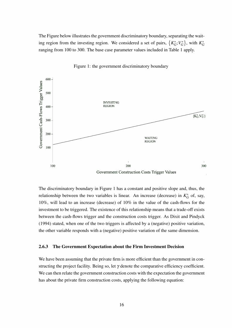
The Figure below illustrates the government discriminatory boundary, separating the wait-ing region from the investing region. We considered a set of pairs,

{K∗G;V ∗G

}, with K∗G

ranging from 100 to 300. The base case parameter values included in Table 1 apply.

Figure 1: the government discriminatory boundary

The discriminatory boundary in Figure 1 has a constant and positive slope and, thus, therelationship between the two variables is linear. An increase (decrease) in K∗G of, say,10%, will lead to an increase (decrease) of 10% in the value of the cash-flows for theinvestment to be triggered. The existence of this relationship means that a trade-off existsbetween the cash-flows trigger and the construction costs trigger. As Dixit and Pindyck(1994) stated, when one of the two triggers is affected by a (negative) positive variation,the other variable responds with a (negative) positive variation of the same dimension.

2.6.3 The Government Expectation about the Firm Investment Decision

We have been assuming that the private firm is more efficient than the government in con-structing the project facility. Being so, let γ denote the comparative efficiency coefficient.We can then relate the government construction costs with the expectation the governmenthas about the private firm construction costs, applying the following equation:

16

KP = KG(1− γ) (13)

We now proceed to compute the trigger values of the private firm as estimated by thegovernment. The firm may face a penalty cost, which we denote by c, for delaying theinitiation of the project. This means that - even though flexibility concerning the timingto implement the project is present - such flexibility implies a cost, as we have stressed.Let FP(VP,KP) denote the government expectation about the value of the private firm in-vestment opportunity. Under risk-neutrality, FP(VP,KP) must satisfy the following partialdifferential equation:

12

σ2VP

V 2P

∂ 2FP

∂V 2P+

12

σ2KP

K2P

∂ 2FP

∂K2P+ρPσVPσKPVPKP

∂ 2FP

∂VP∂KP+

(r−δVP)VP∂FP

∂VP+(r−δKP)

∂FP

∂KP− rFP− c = 0 (14)

Equation (14) has a non-homogeneous part, c and the rest of the equation is homoge-neous. We reach the general solution for the homogeneous part of the partial differentialequation (14) by applying the same reasoning as in the previous case, i.e., the governmentinvestment decision. Being so, the general solution for the homogeneous part of equation(14), FH

P (VP,KP) takes the form:

FHP (VP,KP) = A5V β+

P Kη+

P +A6V β+

P Kη−

P +A7V β−

P Kη+

P +A8V β−

P Kη−

P (15)

As in the previous case, we are only interested in the pair of roots {β+,η−}, whichsimplifies the solution given by equation (15). Hence, we reach a reduced solution, givenby the following equation:

FHP (VP,KP) = A6V β+

P Kη−

P (16)

The particular solution we propose for the non-homogeneous part, FNHP is:

FNHP = −c

r(17)

17

Stitching together the homogeneous and non-homogeneous solutions, we obtain the fol-lowing expression that satisfies the whole partial differential equation (14):

FHP (VP,KP)+FNH

P = FP(VP,KP) = A6V β+

P Kη−

P −cr

(18)

The value-matching condition, in these circumstances, is given by:

FP(V ∗P ,K∗P) = A6V ∗

β+

P K∗η−

P − cr=V ∗P −K∗P (19)

Unfortunately, this value-matching condition does not support homogeneity of degreeone on both sides, which means that β++ η− 6=1. To overcome this problem, we fol-low Adkins and Paxson (2011) quasi-analytical solution by constructing a set of threesimultaneous equations. The first equation is the elliptical equation (20) below, which isequivalent to equation (8):

Q(β ,η) =12

σ2VP

β (β −1)+12

σ2KP

η(η−1)+

ρσVPσKPβη +(r−δVP)β +(r−δKP)η− r = 0 (20)

The other two equations are the two smooth-pasting conditions derived from the value-matching condition, given by equation (19). The first smooth-pasting condition is thefirst-order derivative of the value-matching condition, in respect to V ∗P . After applyingsome rules of calculus, we obtain the first smooth-pasting condition, which is given bythe following equation:

β+(V ∗P −K∗P +

cr) = V ∗P (21)

The second smooth-pasting condition is the first-order derivative of the value matchingcondition, given by equation (19), in respect to K∗P. Likewise, after applying some rulesof calculus, we reach the second smooth-pasting condition, given by equation (22) below:

η−(V ∗P −K∗P +

cr) = −K∗P (22)

18

Firstly, we will consider that c = 0, i.e., we will derive the private firm cash-flows triggeras if no legal penalty was enforced. Being so, as in the case of Adkins and Paxson (2011),we face the existence of four unknowns: V ∗P , K∗P, β+, η− and only three equations areavailable. We will use a set of simultaneous equations, as Adkins and Paxson (2011) didto determine the four uncertains. The set of equations is formed by equations (20), (21)and (22), enabling us to reach new values for V ∗P , β+, η+, after perturbing K∗P. Thus, byapplying this procedure, we determine the firm cash-flows trigger, for a given K∗P, as if nopenalty was enforced. We will designate, from now on, this trigger as V+

P . Hence, V+P

represents the private firm trigger that needs to be moved downwards in order to perfectlymeet the government cash-flows trigger, V ∗G.12 Secondly, we will use the same set ofsimultaneous equations with the purpose of determining the exact value for c that movesV+

P downwards to perfectly meet V ∗G. The value of c that perfectly moves V+P downwards

in order to meet V ∗G is the optimal value for the contractual penalty. Therefore, the optimalcontractual penalty is the one that makes V ∗P = V ∗G for a given K∗P or, which is the same,the one that perfectly aligns both cash-flows triggers. We designate the optimal value forthe contractual penalty as c∗.

2.6.4 Determining the Optimal Value for the Contractual Penalty

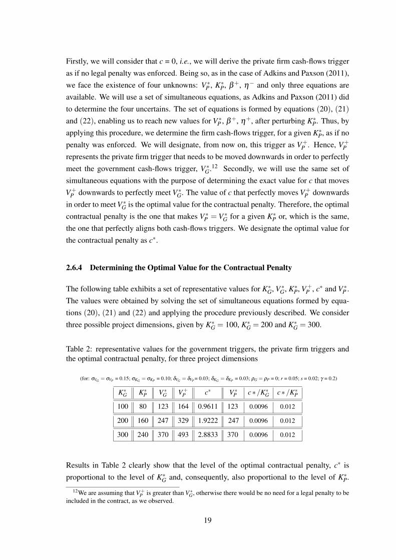
The following table exhibits a set of representative values for K∗G, V ∗G, K∗P, V+P , c∗ and V ∗P .

The values were obtained by solving the set of simultaneous equations formed by equa-tions (20), (21) and (22) and applying the procedure previously described. We considerthree possible project dimensions, given by K∗G = 100, K∗G = 200 and K∗G = 300.

Table 2: representative values for the government triggers, the private firm triggers andthe optimal contractual penalty, for three project dimensions

(for: σVG = σVP = 0.15; σKG = σKP = 0.10; δVG = δVP = 0.03; δKG = δKP = 0.03; ρG = ρP = 0; r = 0.05; s = 0.02; γ = 0.2)

K∗G K∗P V ∗G V+P c∗ V ∗P c∗/K∗G c∗/K∗P

100 80 123 164 0.9611 123 0.0096 0.012

200 160 247 329 1.9222 247 0.0096 0.012

300 240 370 493 2.8833 370 0.0096 0.012

Results in Table 2 clearly show that the level of the optimal contractual penalty, c∗ isproportional to the level of K∗G and, consequently, also proportional to the level of K∗P.

12We are assuming that V+P is greater than V ∗G, otherwise there would be no need for a legal penalty to be

included in the contract, as we observed.

19

This means that no scale-effect is present in the model: an increase (decrease) in the con-struction costs trigger will lead to an increase (decrease) in the value of the optimal legalpenalty of the same magnitude. This proportionality feature allows us to determine thelevel of the optimal contractual penalty “per unit” of the private firm’s expected construc-tion costs which, according to the inputs considered, equals approximately, 0.012.

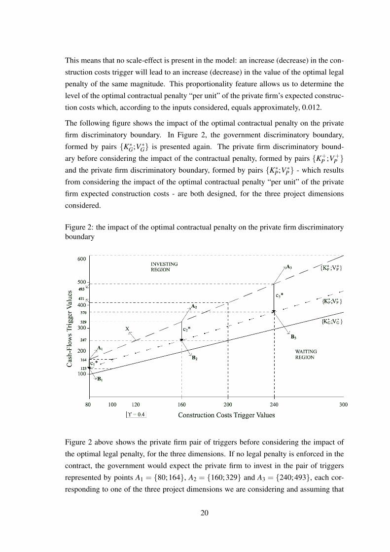
The following figure shows the impact of the optimal contractual penalty on the privatefirm discriminatory boundary. In Figure 2, the government discriminatory boundary,formed by pairs {K∗G;V ∗G} is presented again. The private firm discriminatory bound-ary before considering the impact of the contractual penalty, formed by pairs {K+

P ;V+P }

and the private firm discriminatory boundary, formed by pairs {K∗P;V ∗P} - which resultsfrom considering the impact of the optimal contractual penalty “per unit” of the privatefirm expected construction costs - are both designed, for the three project dimensionsconsidered.

Figure 2: the impact of the optimal contractual penalty on the private firm discriminatoryboundary

Figure 2 above shows the private firm pair of triggers before considering the impact ofthe optimal legal penalty, for the three dimensions. If no legal penalty is enforced in thecontract, the government would expect the private firm to invest in the pair of triggersrepresented by points A1 = {80;164}, A2 = {160;329} and A3 = {240;493}, each cor-responding to one of the three project dimensions we are considering and assuming that

20

the comparative efficiency is γ = 0.2. Thus, by solving the system of simultaneous equa-tions composed by equations (4.20), (4.21) and (4.22), we have reached the three pointsB1 = {80;123}, A2 = {160;247} and A3 = {240;370}. By joining these three points, weobtain another discriminatory boundary: the private firm discriminatory boundary afterconsidering the impact of the optimal contractual penalty, formed by pairs {K∗P;V ∗P}. Infact, points A1, A2 and A3 are three of a countless set of points representing a countlessset of pairs, {K∗P;V ∗P} which define the private firm discriminatory boundary after consid-ering the impact of the contractual penalty. Figure 2 also clearly shows that the privatefirm discriminatory boundary does not match the government discriminatory boundary.In fact, as we have argued, the optimal penalty for each project dimension, c∗1, c∗2 and c∗3is the one that moves the private firm cash-flows trigger downwards in order to perfectlymeet the government cash-flows trigger. This is exactly the effect that each of the opti-mal values for the contractual penalty produce and such effect is represented in Figure 2by three arrows, one for each project dimension. It is visible that the greater the projectdimension the greater the size of the corresponding arrow, hence reflecting that a highercontractual penalty is needed as the project assumes greater dimensions. The private firmdiscriminatory boundary, formed by pairs {K∗P;V ∗P} is then situated between the privatefirm discriminatory boundary before considering the impact of the contractual penalty,formed by pairs {K+

P ;V+P } and the government discriminatory boundary, formed by pairs

{K∗G;V ∗G}.13

Figure 2 also includes a specific point, which we designate as X . This point is situ-ated where the private firm discriminatory boundary, after considering the impact of theoptimal legal penalty (the one composed by pairs {K∗P;V ∗P}), intersects the line for thegovernment cash-flows trigger on the second dimension, i.e., V ∗G = 247. To this projectdimension, the government cash-flows trigger and private firm cash-flows trigger are bothequal to 247 and, to that cash-flows trigger value, corresponds a private firm constructioncosts trigger of K∗P = 120. Hence, considering the second dimension, given by K∗G = 200,the private firm construction costs trigger, K∗P = 120 when the comparative efficiency fac-tor, γ = 0.4. This means that, for this project dimension, if the comparative efficiencyfactor is equal or greater than 0.4, there is no need to include a legal penalty in the con-tract form because the efficiency factor, for a level of social costs equal to 0.02, is strongenough to move the private firm cash-flows trigger downwards in order to perfectly meetthe government cash-flows trigger.

13The private firm discriminatory boundary, after considering the impact of the optimal legal penalty, willonly match the government discriminatory boundary if both entities were equally efficient, i.e., if γ = 0.

21

2.7 Sensitivity Analysis

2.7.1 The Impact of the Level of Social Costs on the Optimal Contractual Penalty

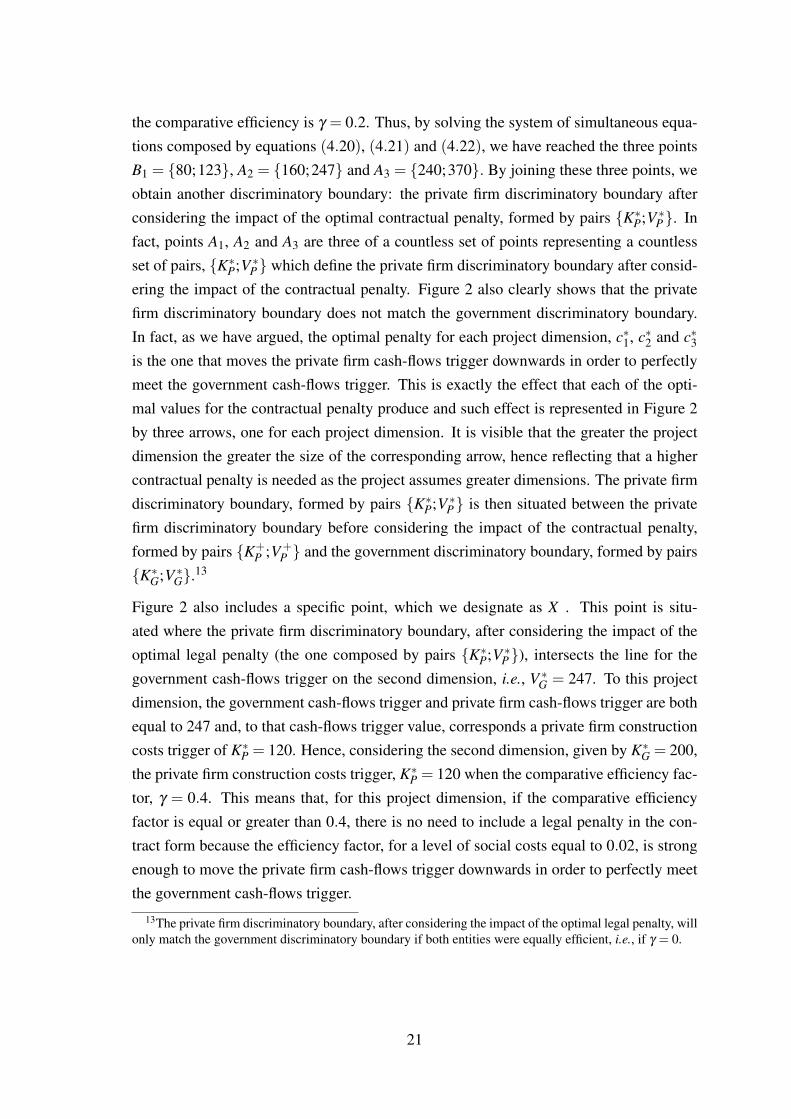
Table 3 includes a set of values for the level of social costs and their impact on the gov-ernment cash-flows trigger and on the optimal contractual penalty, assuming the projectdimension given by K∗G = 200.

Table 3: sensitivity analysis: the impact of the level of social costs on the optimal con-tractual penalty

(for: σVG = σVP = 0.15; σKG = σKP = 0.10; δVG = δVP = 0.03; δKG = δKP = 0.03; ρG = ρP = 0; r = 0.05; γ = 0.2)

K∗G K∗P s V ∗G c∗ V+P V ∗P

200 160 0.00 411 0.0000 329 411

200 160 0.01 308 0.4732 329 308

200 160 0.02 247 1.9222 329 247

200 160 0.03 206 2.9235 329 206

200 160 0.04 176 3.6661 329 176

200 160 0.05 154 4.2443 329 154

Assuming s = 0 , then there is no need for enforcing a legal penalty, since the governmentcash-flows trigger (V ∗G = 411) is placed above the private firm cash-flows trigger, beforeconsidering the effect of any penalty (V+

P = 329). For values of s greater than zero,the higher the level of social costs the more below the government cash-flows trigger issituated, which means that the distance between the private firm cash-flows trigger andthe government cash-flows trigger becomes greater. As a consequence, higher levels forthe contractual penalty are needed to move the private firm cash-flows trigger downwardsand align it with the government cash-flows trigger.

2.7.2 The Impact of the Efficiency Factor on the Optimal Contractual Penalty

Table 4 includes a set of different values for the comparative efficiency factor and theirimpact on the optimal contractual penalty, assuming that the project dimension is givenby K∗G = 200.

22

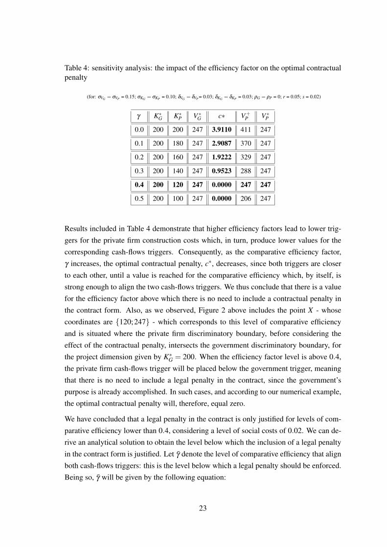
Table 4: sensitivity analysis: the impact of the efficiency factor on the optimal contractualpenalty

(for: σVG = σVP = 0.15; σKG = σKP = 0.10; δVG = δVP = 0.03; δKG = δKP = 0.03; ρG = ρP = 0; r = 0.05; s = 0.02)

γ K∗G K∗P V ∗G c∗ V+P V ∗P

0.0 200 200 247 3.9110 411 247

0.1 200 180 247 2.9087 370 247

0.2 200 160 247 1.9222 329 247

0.3 200 140 247 0.9523 288 247

0.4 200 120 247 0.0000 247 247

0.5 200 100 247 0.0000 206 247

Results included in Table 4 demonstrate that higher efficiency factors lead to lower trig-gers for the private firm construction costs which, in turn, produce lower values for thecorresponding cash-flows triggers. Consequently, as the comparative efficiency factor,γ increases, the optimal contractual penalty, c∗, decreases, since both triggers are closerto each other, until a value is reached for the comparative efficiency which, by itself, isstrong enough to align the two cash-flows triggers. We thus conclude that there is a valuefor the efficiency factor above which there is no need to include a contractual penalty inthe contract form. Also, as we observed, Figure 2 above includes the point X - whosecoordinates are {120;247} - which corresponds to this level of comparative efficiencyand is situated where the private firm discriminatory boundary, before considering theeffect of the contractual penalty, intersects the government discriminatory boundary, forthe project dimension given by K∗G = 200. When the efficiency factor level is above 0.4,the private firm cash-flows trigger will be placed below the government trigger, meaningthat there is no need to include a legal penalty in the contract, since the government’spurpose is already accomplished. In such cases, and according to our numerical example,the optimal contractual penalty will, therefore, equal zero.

We have concluded that a legal penalty in the contract is only justified for levels of com-parative efficiency lower than 0.4, considering a level of social costs of 0.02. We can de-rive an analytical solution to obtain the level below which the inclusion of a legal penaltyin the contract form is justified. Let γ̄ denote the level of comparative efficiency that alignboth cash-flows triggers: this is the level below which a legal penalty should be enforced.Being so, γ̄ will be given by the following equation:

23

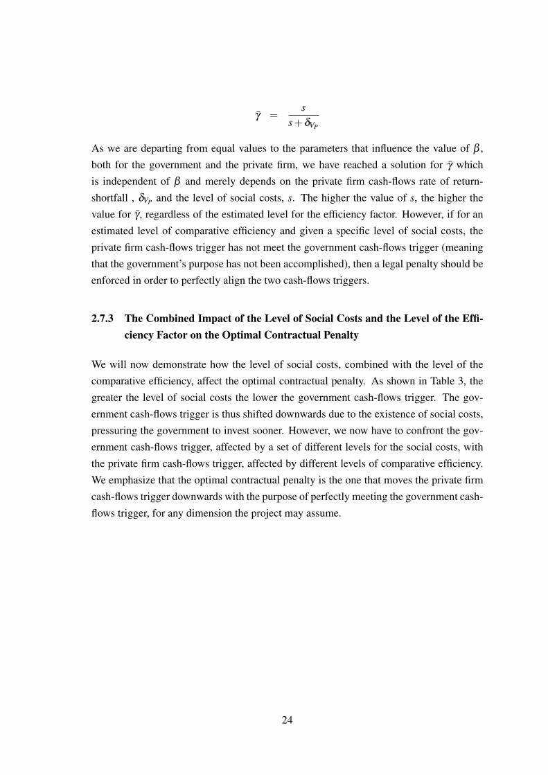
γ̄ =s

s+δVP

As we are departing from equal values to the parameters that influence the value of β ,both for the government and the private firm, we have reached a solution for γ̄ whichis independent of β and merely depends on the private firm cash-flows rate of return-shortfall , δVP and the level of social costs, s. The higher the value of s, the higher thevalue for γ̄ , regardless of the estimated level for the efficiency factor. However, if for anestimated level of comparative efficiency and given a specific level of social costs, theprivate firm cash-flows trigger has not meet the government cash-flows trigger (meaningthat the government’s purpose has not been accomplished), then a legal penalty should beenforced in order to perfectly align the two cash-flows triggers.

2.7.3 The Combined Impact of the Level of Social Costs and the Level of the Effi-ciency Factor on the Optimal Contractual Penalty

We will now demonstrate how the level of social costs, combined with the level of thecomparative efficiency, affect the optimal contractual penalty. As shown in Table 3, thegreater the level of social costs the lower the government cash-flows trigger. The gov-ernment cash-flows trigger is thus shifted downwards due to the existence of social costs,pressuring the government to invest sooner. However, we now have to confront the gov-ernment cash-flows trigger, affected by a set of different levels for the social costs, withthe private firm cash-flows trigger, affected by different levels of comparative efficiency.We emphasize that the optimal contractual penalty is the one that moves the private firmcash-flows trigger downwards with the purpose of perfectly meeting the government cash-flows trigger, for any dimension the project may assume.

24

Table 5: sensitivity analysis: the combined impact of the level of social costs and the levelof the efficiency factor on the optimal contractual penalty

(for: σVG = σVP = 0.15; σKG = σKP = 0.10; δVG = δVP = 0.03; δKG = δKP = 0.03; ρG = ρP = 0; r = 0.05)

s=0.01 s=0.02 s=0.03 s=0.04 s=0.05

γ=0.1 1.4311 2.9087 3.9359 4.7014 5.2996

γ=0.2 0.4734 1.9222 2.9235 3.6661 4.2443

γ=0.3 0.0000 0.9523 1.9290 2.6494 3.2078

γ=0.4 0.000 0.0000 0.0000 1.6535 2.1926

γ=0.5 0.000 0.0000 0.000 0.6802 1.2013

The values included in Table 5 are the optimal penalty values that result from consideringcombinations for the level of social costs and for the level of the efficiency factor. Theresults clearly illustrate what we have been arguing: the greater the level of social coststhe higher the value of the optimal legal penalty and, the higher the efficiency factor, thelower the value of the optimal penalty. However, when the comparative efficiency factoris equal to or higher than 0.4 and the level of social costs is equal to or lower than 0.03,there is no need to impose a legal penalty in the contract form because the combinationof the two factors is strong enough to align the two cash-flows triggers. The same alsohappens when γ = 0.3 and s = 0.01. This is the reason why, in such cases, the optimalcontractual penalty included in Table 5 is zero.

2.7.4 The Impact of Variations in the Correlation Coefficients on the Optimal Con-tractual Penalty

We have been assuming that the correlation coefficient, ρ is zero and, hence, all calcula-tions were made considering the absence of correlation between the facility constructioncosts and the present value of cash-flows to be generated from subsequent operations.Table 6 includes the results of the impact on the optimal contractual penalty caused byvariations in both correlation coefficients, ρG and ρP, assuming γ = 0.2 and s = 0.02. Weshould stress that any change in ρG will cause the roots that are extracted from equation(8) to change and, thus, V ∗G will also change. The impact on V+

P is also presented. We setK∗G to 200 and the conclusions are equivalent for any other level of K∗G, since the resultsincluded in Table 2 demonstrate the existence of proportionality between this trigger and

25

the optimal level for the contractual penalty, c∗.14

Table 6: the impact of variations in the correlation coefficients on the optimal contractualpenalty

(for: σVG = σVP = 0.15; σKG = σKP = 0.10; δVG = δVP = 0.03; δKG = δKP = 0.03; r = 0.05; s = 0.02; γ = 0.2)

(ρG;ρP) (-1.0;-1.0) (-0.5;-0.5) (0.0;0.0) (0.5;0.5) (1.0;1.0)

K∗G 200 200 200 200 200

V ∗G 320 284 247 205 147

V+P 427 379 329 273 196

V ∗P 320 284 247 205 147

c∗ 2.3213 2.1295 1.9222 1.6791 1.1967

Results in Table 6 show that one should expect that, as the correlation coefficients in-crease, from (−1.0;−1.0) to (1.0;1.0), the value of the optimal legal penalty would de-crease, since stronger positive (or less negative) correlations lead to lower cash-flowstrigger values, both for the government and the private firm. It is expected that increasingpositive (or less decreasing negative) correlations would result in lower cash-flows trig-gers for both entities. If, say, construction costs rise 20 and ρ = 0.5, thus the cash-flowswill, expectedly, rise 10, which means that the cash-flows trigger will be lower. If, for thesame variation in the construction costs, the cash-flows rise more than 10 (which meansthat ρ > 0.5), then one would expect that the cash-flows trigger value would be even lowerthan in the previous example. Triggers will, therefore, be closer to each other as positive(or less negative) correlations become greater and the differences between the triggers be-come smaller. And, since the difference between the triggers will be smaller, one wouldexpect that a lower value for the contractual penalty will be sufficient to perfectly alignthem. On the contrary, higher negative correlations (or lower positive correlations) will,expectedly, result in greater differences between the private firm cash-flows trigger - inthe event that no penalty is enforced - and the government cash-flows trigger, meaningthat, in these circumstances, a greater value for the legal penalty will be needed in orderto move the firm cash-flows trigger downwards and perfectly align it with the governmentcash-flows trigger, for each value the correlation coefficient may assume.

14In order to confirm the existence of this proportionality, we set K∗G to 100 and reached optimal penaltyvalues, for all levels of ρ , half as great as the ones included in Table 6. These results demonstrate theexistence of proportionality between K∗G and c∗, as the results included in Table 2 demonstrate.

26

2.7.5 The Impact of Changes in the Standard Deviations on the Optimal Contrac-tual Penalty

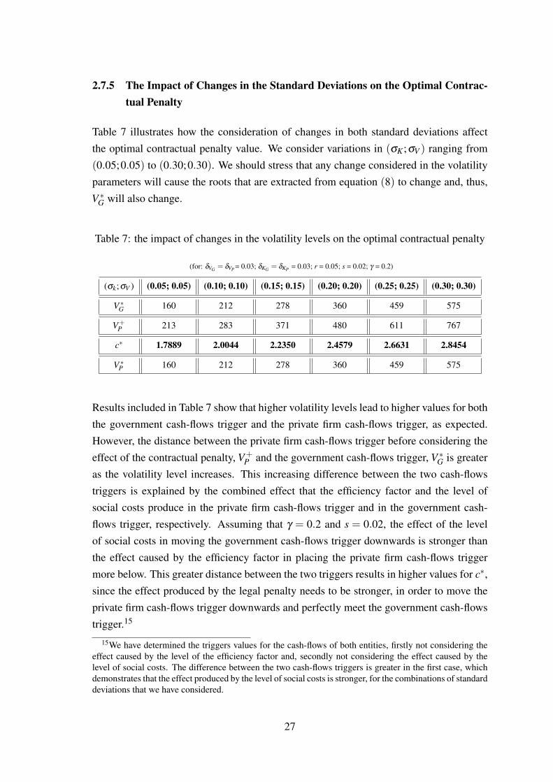
Table 7 illustrates how the consideration of changes in both standard deviations affectthe optimal contractual penalty value. We consider variations in (σK;σV ) ranging from(0.05;0.05) to (0.30;0.30). We should stress that any change considered in the volatilityparameters will cause the roots that are extracted from equation (8) to change and, thus,V ∗G will also change.

Table 7: the impact of changes in the volatility levels on the optimal contractual penalty

(for: δVG = δVP = 0.03; δKG = δKP = 0.03; r = 0.05; s = 0.02; γ = 0.2)

(σk;σV ) (0.05; 0.05) (0.10; 0.10) (0.15; 0.15) (0.20; 0.20) (0.25; 0.25) (0.30; 0.30)

V ∗G 160 212 278 360 459 575

V+P 213 283 371 480 611 767

c∗ 1.7889 2.0044 2.2350 2.4579 2.6631 2.8454

V ∗P 160 212 278 360 459 575

Results included in Table 7 show that higher volatility levels lead to higher values for boththe government cash-flows trigger and the private firm cash-flows trigger, as expected.However, the distance between the private firm cash-flows trigger before considering theeffect of the contractual penalty, V+

P and the government cash-flows trigger, V ∗G is greateras the volatility level increases. This increasing difference between the two cash-flowstriggers is explained by the combined effect that the efficiency factor and the level ofsocial costs produce in the private firm cash-flows trigger and in the government cash-flows trigger, respectively. Assuming that γ = 0.2 and s = 0.02, the effect of the levelof social costs in moving the government cash-flows trigger downwards is stronger thanthe effect caused by the efficiency factor in placing the private firm cash-flows triggermore below. This greater distance between the two triggers results in higher values for c∗,since the effect produced by the legal penalty needs to be stronger, in order to move theprivate firm cash-flows trigger downwards and perfectly meet the government cash-flowstrigger.15

15We have determined the triggers values for the cash-flows of both entities, firstly not considering theeffect caused by the level of the efficiency factor and, secondly not considering the effect caused by thelevel of social costs. The difference between the two cash-flows triggers is greater in the first case, whichdemonstrates that the effect produced by the level of social costs is stronger, for the combinations of standarddeviations that we have considered.

27

3 The Effects, to the Government, of a Including a Non-Optimal Value for the

Legal Penalty in the Contract

The model described proposes a method to determine the optimal level for the contractualpenalty, from the government perspective. Based on its own estimates about the facilityconstruction costs and the value of cash-flows to be generated from running the subse-quent operations, and estimating the level of social costs and the comparative efficiencyfactor, the government is able to reach the value for the optimal contractual penalty “perunit” of the private firm’s expected cost. This optimal contractual penalty moves theprivate firm cash-flows trigger downwards in order to meet the government cash-flowstrigger. However, as we are considering the government facility construction costs to bestochastic, one may legitimately ask which value for the government construction costsshould the government consider for the purpose of determining the optimal penalty to beincluded in the contract form, in the day the optimal contractual penalty needs to be de-termined. Since any rational agent makes decisions based on the best information he orshe has in the specific moment the decisions need to be taken, we can conclude that theestimated value for the construction costs the government has computed in that same mo-ment will be the value the government should use for the purpose of determining the op-timal contractual penalty. However, since the government construction costs, KG behavestochastically, their value might be different the day after the day the value for the contrac-tual penalty was determined. If such occurs, the value of the legal penalty determined andincluded in the contract form the day before will no longer be optimal. However, since thegovernment needs to make a decision, the optimal value for the contractual penalty, onthat day, is determined by the government, based on the expected construction costs esti-mated on that same day, and included in the contract form. Sometime after, a competitivebid takes place. All bidders have access to this crucial information since the contractualrules are included in the bid documents provided to all the participants. Bidders preparetheir proposals taking into account the presence of this contractual penalty and define theirbid prices accordingly. One of the bidders is selected and invited to sign the contract and,consequently, to invest in executing the project facility and run the subsequent activities.

Yet, one may consider that the value of the legal penalty included in the contract form isnot optimal - not only due to the fact the government construction costs behave stochas-tically, as we just mentioned - but also because the government might have inaccuratelyestimated the selected bidder comparative efficiency. In fact, it is possible that the gov-ernment has determined the value of the contractual penalty assuming a comparative ef-ficiency factor which is different from the selected bidder’s real comparative efficiency.Being so, we should examine the effects that overestimating or underestimating the effi-

28

ciency factor will produce, from the government’s perspective. For this purpose, we needto present the value of the selected bidder investment opportunity.

Let FB(VB,KB) denote the value of the selected bidder option to invest in a project wherea legal penalty will be enforced in the case the selected firm does not implement theproject immediately. VB designates the present value of the cash-flows the selected bid-der will generate by running the activities and KB designates the selected bidder facilityconstruction costs. Considering the same assumptions we have considered when we de-rived FP(VP,KP), i.e., the government expectation about the private firm decision to invest,and applying the same procedure, we then reach the boundary that separates the selectedbidder’s waiting and investing regions.16

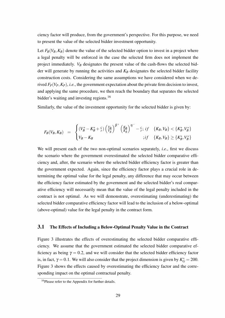
Similarly, the value of the investment opportunity for the selected bidder is given by:

FB(VB,KB) =

(V ∗B −K∗B +cr )(

VBV ∗B

)β+ (KBK∗B

)η−

− cr ; i f {KB,VB}< {K∗B,V ∗B}

VB−KB ; i f {KB,VB} ≥ {K∗B,V ∗B}

We will present each of the two non-optimal scenarios separately, i.e., first we discussthe scenario where the government overestimated the selected bidder comparative effi-ciency and, after, the scenario where the selected bidder efficiency factor is greater thanthe government expected. Again, since the efficiency factor plays a crucial role in de-termining the optimal value for the legal penalty, any difference that may occur betweenthe efficiency factor estimated by the government and the selected bidder’s real compar-ative efficiency will necessarily mean that the value of the legal penalty included in thecontract is not optimal. As we will demonstrate, overestimating (underestimating) theselected bidder comparative efficiency factor will lead to the inclusion of a below-optimal(above-optimal) value for the legal penalty in the contract form.

3.1 The Effects of Including a Below-Optimal Penalty Value in the Contract

Figure 3 illustrates the effects of overestimating the selected bidder comparative effi-ciency. We assume that the government estimated the selected bidder comparative ef-ficiency as being γ = 0.2, and we will consider that the selected bidder efficiency factoris, in fact, γ = 0.1. We will also consider that the project dimension is given by K∗G = 200.Figure 3 shows the effects caused by overestimating the efficiency factor and the corre-sponding impact on the optimal contractual penalty.

16Please refer to the Appendix for further details.

29

Figure 3: the impact of overestimating the comparative efficiency on the optimal contrac-tual penalty

In Figure 3, point A2 has the coordinates that correspond to the selected bidder pair of trig-gers before considering the effect of the contractual penalty, assuming the efficiency factorestimated by the government, i.e, {K+

B ;V+B } = {160;329}, whereas point B2 graphically

represents the selected bidder pair of triggers, {K∗B;V ∗B} = {160;329} after consideringthe impact of the legal penalty enforced in the contract, c2 = 1.9222. In these circum-stances, the government would expect the value of legal penalty included in the contractform, c2 to be sufficiently strong in moving the selected bidder cash-flows trigger down-wards, from V+

B = 329 to V ∗B = 247 and, thus, perfectly meet the government cash-flowstrigger, V ∗G = 247. By overestimating the efficiency factor, the government has not suc-ceeded in reaching such purpose. The government was expecting the selected bidder totrigger the investment in {K∗B;V ∗B} = {160;247}, represented by point B2, as the resultof enforcing the contractual penalty, c2 = 1.9222. If no penalty was enforced, the se-lected bidder would invest in point A

′2 , whose coordinates are {K+

B ;V+B } = {180;370}.

By enforcing the contractual penalty c2 = 1.9222 when the selected bidder comparativeefficiency is γ = 0.1, the government is leading the selected bidder to invest in point B’

2,whose coordinates are {K∗B;V ∗B} = {180;288}. In fact, the selected bidder constructioncosts trigger, considering his or her real comparative efficiency, is K∗B = 180, and the cor-responding cash-flows trigger is V ∗B = 288.17 Thus, by imposing the contractual penalty,

17For a given value of the selected bidder construction costs trigger, the corresponding cash-flows trigger

30

c2 = 1.9222, the government has caused the selected bidder cash-flows trigger to movefrom V+

B = 370 to V ∗B = 288. Hence, the government’s purpose of moving the selectedfirm cash-flows trigger downwards to perfectly meet the government cash-flows triggerhas not been accomplished, since the selected bidder cash-flows trigger is higher thanthe government cash-flows trigger. This means that a greater penalty value is needed tomove further downwards0the selected bidder cash-flows trigger. In Figure 3, the optimalcontractual penalty is given by c∗2 and is clearly visible that the line segment reflectingthe impact of the optimal contractual penalty, c∗2 is bigger than the line segment that re-flects the impact caused by the value of the legal penalty actually included in the contract,c2 = 1.9222. This fact graphically illustrates that overestimating the comparative effi-ciency factor leads to the definition of a below-optimal value for the contractual penalty.

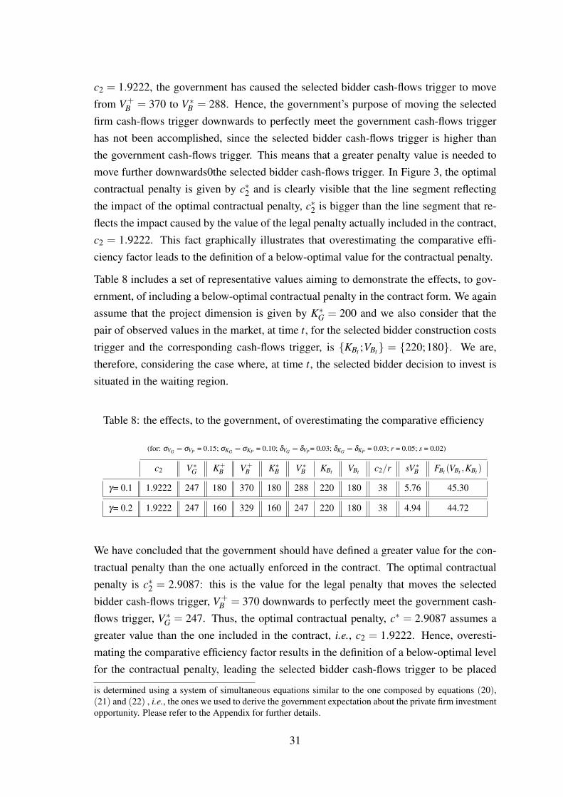
Table 8 includes a set of representative values aiming to demonstrate the effects, to gov-ernment, of including a below-optimal contractual penalty in the contract form. We againassume that the project dimension is given by K∗G = 200 and we also consider that thepair of observed values in the market, at time t, for the selected bidder construction coststrigger and the corresponding cash-flows trigger, is {KBt ;VBt} = {220;180}. We are,therefore, considering the case where, at time t, the selected bidder decision to invest issituated in the waiting region.

Table 8: the effects, to the government, of overestimating the comparative efficiency

(for: σVG = σVP = 0.15; σKG = σKP = 0.10; δVG = δVP = 0.03; δKG = δKP = 0.03; r = 0.05; s = 0.02)

c2 V ∗G K+B V+

B K∗B V ∗B KBt VBt c2/r sV ∗B FBt (VBt ,KBt )

γ= 0.1 1.9222 247 180 370 180 288 220 180 38 5.76 45.30

γ= 0.2 1.9222 247 160 329 160 247 220 180 38 4.94 44.72

We have concluded that the government should have defined a greater value for the con-tractual penalty than the one actually enforced in the contract. The optimal contractualpenalty is c∗2 = 2.9087: this is the value for the legal penalty that moves the selectedbidder cash-flows trigger, V+

B = 370 downwards to perfectly meet the government cash-flows trigger, V ∗G = 247. Thus, the optimal contractual penalty, c∗ = 2.9087 assumes agreater value than the one included in the contract, i.e., c2 = 1.9222. Hence, overesti-mating the comparative efficiency factor results in the definition of a below-optimal levelfor the contractual penalty, leading the selected bidder cash-flows trigger to be placed

is determined using a system of simultaneous equations similar to the one composed by equations (20),(21) and (22) , i.e., the ones we used to derive the government expectation about the private firm investmentopportunity. Please refer to the Appendix for further details.

31

above the government cash-flows trigger. In fact, by setting the government constructioncosts, K∗G = 200, the selected bidder construction costs trigger is K∗B = 180 for γ = 0.1and its cash-flows trigger, V ∗B = 288, considering the value of the penalty included in thecontract form, c2 = 1.9222. Since the selected bidder will have a higher cash-flows trig-ger than the government predicted, the value of social costs will be beyond the level thegovernment considers to be acceptable. The government was prepared to accept socialcosts of s = 4.94 in our example but, because the cash-flows trigger value is higher thanthe government expected, the selected bidder is causing the social costs to be s = 5.76,which means that the population will have to bear an additional value of social costs ofs = 0.82. Yet, the fact that the contractual penalty is below its optimal level results ina more valuable option to invest for the selected bidder “vis-a-vis” with the scenariowhere the contractual penalty written down in the contract is optimal. The informa-tion included in Table 8 confirms such. Assuming that the pair of observed values, attime t, {KBt ;VBt} = {220;180}, the value of the selected bidder investment opportunity,FB(KB,VB), at time t equals 45.30, whereas FB(KB,VB), at time t, in the scenario wherethe legal penalty written down in the contract is optimal, equals 44.72. This numericallydemonstrates that the value of the option to invest is more valuable in the presence of abelow-optimal contractual penalty. Since we believe that rational bidders will offer higherprices as a direct consequence of holding a more valuable option to invest, the governmentwould, therefore, receive a higher price. However, the additional revenue the governmentwould receive would also entail a cost: the higher value of social costs the populationwould have to bear. We argue that the government would prefer to receive a lower priceand ensure that the value of social costs, previously defined as being tolerable, wouldnot be exceeded. Hence, the scenario where a below-optimal contractual penalty valueis considered will produce effects, to the government, which we believe the governmentwould prefer to avoid.

3.2 The Effects of Including an Above-Optimal Penalty Value in the Contract

Figure 4 illustrates the impact of underestimating the selected bidder comparative effi-ciency on the optimal contractual penalty. We assume, in this scenario, that the selectedbidder efficiency factor is, in fact, γ = 0.3. Like in the previous scenario, we consider thatthe project dimension is given by K∗G = 200.

32

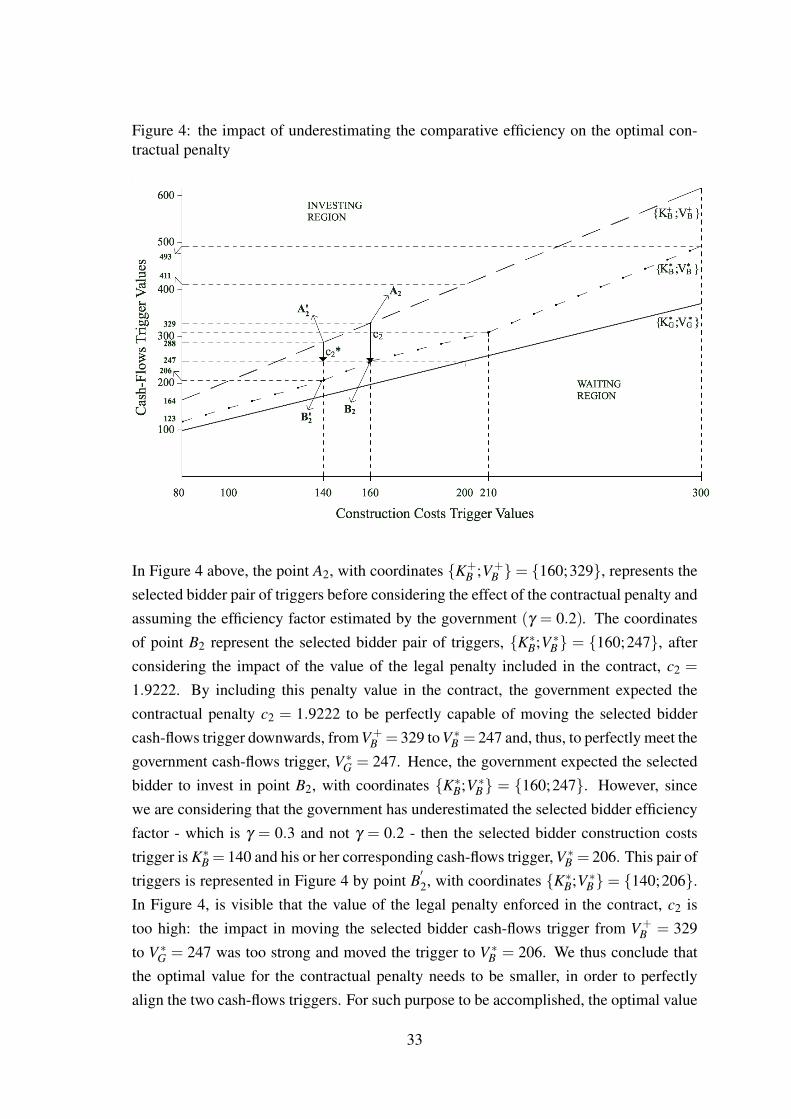
Figure 4: the impact of underestimating the comparative efficiency on the optimal con-tractual penalty

In Figure 4 above, the point A2, with coordinates {K+B ;V+

B }= {160;329}, represents theselected bidder pair of triggers before considering the effect of the contractual penalty andassuming the efficiency factor estimated by the government (γ = 0.2). The coordinatesof point B2 represent the selected bidder pair of triggers, {K∗B;V ∗B} = {160;247}, afterconsidering the impact of the value of the legal penalty included in the contract, c2 =

1.9222. By including this penalty value in the contract, the government expected thecontractual penalty c2 = 1.9222 to be perfectly capable of moving the selected biddercash-flows trigger downwards, from V+

B = 329 to V ∗B = 247 and, thus, to perfectly meet thegovernment cash-flows trigger, V ∗G = 247. Hence, the government expected the selectedbidder to invest in point B2, with coordinates {K∗B;V ∗B} = {160;247}. However, sincewe are considering that the government has underestimated the selected bidder efficiencyfactor - which is γ = 0.3 and not γ = 0.2 - then the selected bidder construction coststrigger is K∗B = 140 and his or her corresponding cash-flows trigger, V ∗B = 206. This pair oftriggers is represented in Figure 4 by point B

′2, with coordinates {K∗B;V ∗B} = {140;206}.

In Figure 4, is visible that the value of the legal penalty enforced in the contract, c2 istoo high: the impact in moving the selected bidder cash-flows trigger from V+

B = 329to V ∗G = 247 was too strong and moved the trigger to V ∗B = 206. We thus conclude thatthe optimal value for the contractual penalty needs to be smaller, in order to perfectlyalign the two cash-flows triggers. For such purpose to be accomplished, the optimal value

33

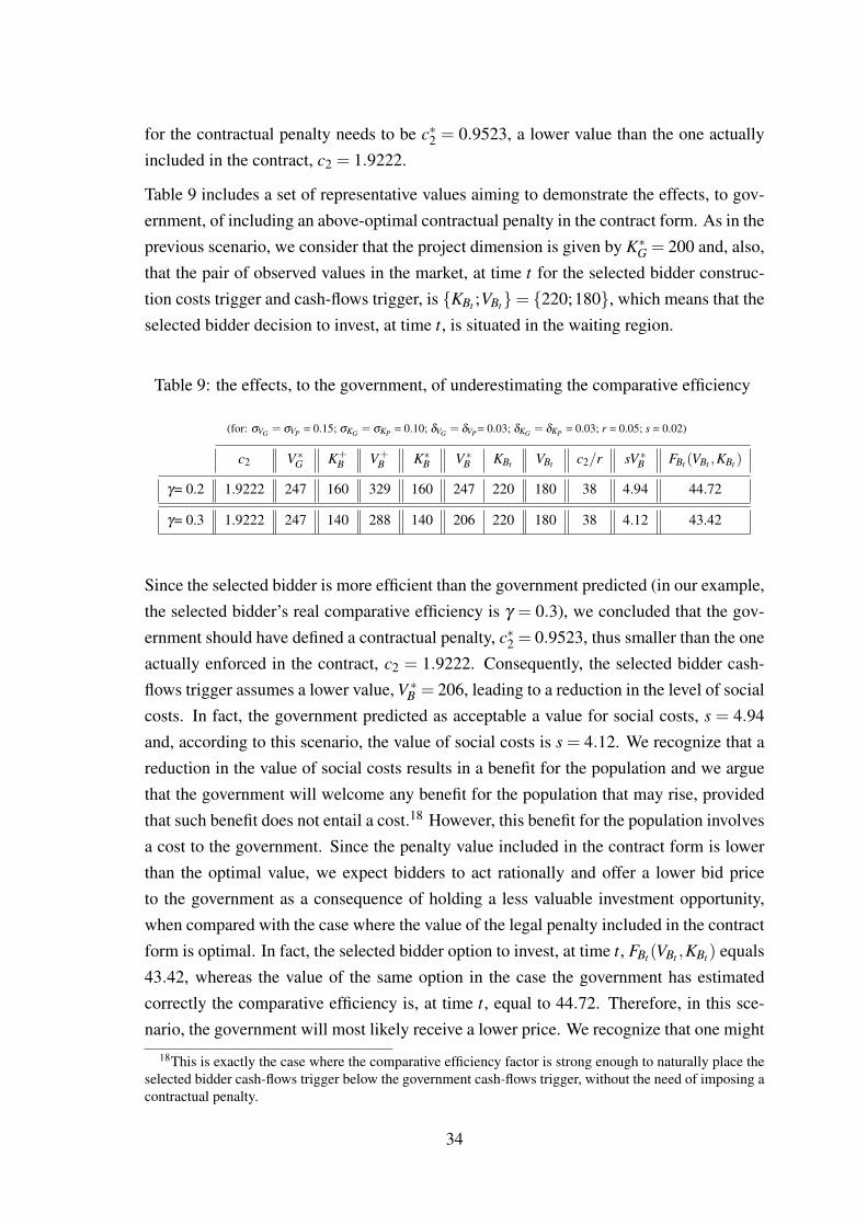
for the contractual penalty needs to be c∗2 = 0.9523, a lower value than the one actuallyincluded in the contract, c2 = 1.9222.

Table 9 includes a set of representative values aiming to demonstrate the effects, to gov-ernment, of including an above-optimal contractual penalty in the contract form. As in theprevious scenario, we consider that the project dimension is given by K∗G = 200 and, also,that the pair of observed values in the market, at time t for the selected bidder construc-tion costs trigger and cash-flows trigger, is {KBt ;VBt}= {220;180}, which means that theselected bidder decision to invest, at time t, is situated in the waiting region.

Table 9: the effects, to the government, of underestimating the comparative efficiency

(for: σVG = σVP = 0.15; σKG = σKP = 0.10; δVG = δVP = 0.03; δKG = δKP = 0.03; r = 0.05; s = 0.02)

c2 V ∗G K+B V+

B K∗B V ∗B KBt VBt c2/r sV ∗B FBt (VBt ,KBt )

γ= 0.2 1.9222 247 160 329 160 247 220 180 38 4.94 44.72

γ= 0.3 1.9222 247 140 288 140 206 220 180 38 4.12 43.42

Since the selected bidder is more efficient than the government predicted (in our example,the selected bidder’s real comparative efficiency is γ = 0.3), we concluded that the gov-ernment should have defined a contractual penalty, c∗2 = 0.9523, thus smaller than the oneactually enforced in the contract, c2 = 1.9222. Consequently, the selected bidder cash-flows trigger assumes a lower value, V ∗B = 206, leading to a reduction in the level of socialcosts. In fact, the government predicted as acceptable a value for social costs, s = 4.94and, according to this scenario, the value of social costs is s = 4.12. We recognize that areduction in the value of social costs results in a benefit for the population and we arguethat the government will welcome any benefit for the population that may rise, providedthat such benefit does not entail a cost.18 However, this benefit for the population involvesa cost to the government. Since the penalty value included in the contract form is lowerthan the optimal value, we expect bidders to act rationally and offer a lower bid priceto the government as a consequence of holding a less valuable investment opportunity,when compared with the case where the value of the legal penalty included in the contractform is optimal. In fact, the selected bidder option to invest, at time t, FBt (VBt ,KBt ) equals43.42, whereas the value of the same option in the case the government has estimatedcorrectly the comparative efficiency is, at time t, equal to 44.72. Therefore, in this sce-nario, the government will most likely receive a lower price. We recognize that one might

18This is exactly the case where the comparative efficiency factor is strong enough to naturally place theselected bidder cash-flows trigger below the government cash-flows trigger, without the need of imposing acontractual penalty.

34

consider that the decrease in the bid price the selected bidder will probably offer actuallycompensates the benefit that derives from the reduction in the value of social costs (thisreduction is equal to 0.82). However, we argue that the government will prefer to accept ahigher level of social costs until the level determined has being tolerable in the first place,and not expose itself to the possibility of incurring in the loss that results from receivinga lower bid price than the one the government would receive, if the value of the legalpenalty included in the contract was, in fact, optimal.

Part III

Conclusions

The suggested model is based on a contractual framework, in the context of a BOT project,where the government grants leeway to the selected bidder regarding the timing of theproject implementation. However, this flexibility may entail a cost, since a legal penaltyis contractual enforced if the selected bidder does not implement the project immediately.Aiming to determine the optimal value for this contractual penalty, we applied a two-factor uncertainty approach, where both the facility construction costs and the presentvalue of cash-flows to be generated by subsequent operations follow Geometric BrownianMotions that are possibly correlated.

We have assumed that the government is less efficient than the private firm in constructingthe project facility and we have also considered the existence of social costs, i.e., thecosts that correspond to the loss of social welfare occurred from the moment the projectshould have been implemented and services being provided to its users and the momentthe project is actually completed. The government’s purpose is to ensure that the selectedbidder will invest when his or her cash-flows trigger has the same value of the governmentcash-flows trigger, if the government decided to conduct the project.

To determine the optimal level for the contractual penalty, we derived the government de-cision to invest and the government expectation about the private firm decision to invest.As the later does not support homogeneity of degree one in the corresponding boundaryconditions, due to the consideration of the legal penalty in the value of the investmentopportunity, we followed Adkins and Paxson (2011) solution and constructed a set ofthree simultaneous equations, which enabled us to define the private firm discriminatoryboundary, i.e., the boundary that separates the private firm’s waiting region from the pri-vate firm’s investing region. We then reached an optimal level for the contractual penalty

35

“per unit” of cost, since there is proportionality between the optimal value for the con-tractual penalty and the value assumed by the facility construction costs.

Sensitivity analysis performed demonstrated that the greater the level of social costs thesooner one expects the government would invest, since the consideration of higher levelsof social costs result in lower values for the government cash-flows trigger. The analysisalso revealed that there is a level for the comparative efficiency above which there is noneed to include a penalty in the contract, since such level of efficiency factor, for the levelof social costs considered, naturally moves the private firm cash-flows trigger downwardsto perfectly meet the government cash-flows trigger. Sensitivity analysis also led us toconclude that changes in the correlation coefficients have a strong expected impact on theoptimal contractual penalty. As both coefficients assume greater values, the value of theoptimal penalty decreases since one expects that stronger correlations will lead to lowercash-flows triggers, both for the government and the private entity.

Finally, we examined the effects that overestimating or underestimating the comparativeefficiency factor produces in the value of the optimal contractual penalty. We concludedthat overestimating the efficiency factor results in the determination of a below-optimalvalue for the contractual penalty, and that underestimating this same factor will lead to theinclusion of an-above optimal value for the legal penalty in the contract form. Being so,since overestimating (underestimating) the value for the comparative efficiency factor willresult in the inclusion of a below-optimal (above-optimal) value for the legal penalty inthe contract, then the selected bidder cash-flows trigger will be greater (smaller) than thegovernment cash-flows trigger. Since the optimal penalty is defined as being the one thatensures the selected firm has the same cash-flows trigger the government would have, ifthe government decided to undertake the project, we then concluded that the government’spurpose will never be accomplished if the comparative efficiency factor is not estimatedwith full accuracy.

36

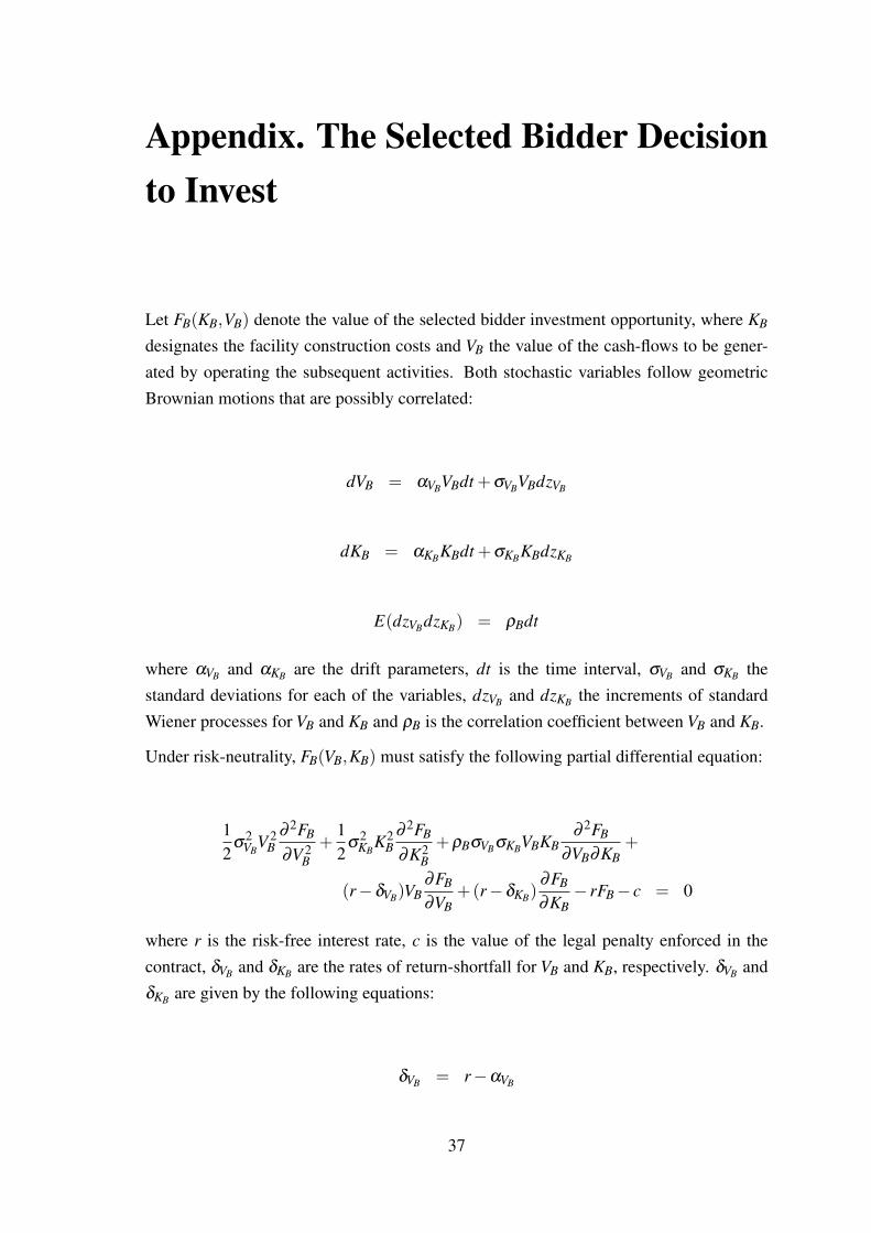
Appendix. The Selected Bidder Decisionto Invest

Let FB(KB,VB) denote the value of the selected bidder investment opportunity, where KB

designates the facility construction costs and VB the value of the cash-flows to be gener-ated by operating the subsequent activities. Both stochastic variables follow geometricBrownian motions that are possibly correlated:

dVB = αVBVBdt +σVBVBdzVB

dKB = αKBKBdt +σKBKBdzKB

E(dzVBdzKB) = ρBdt

where αVB and αKB are the drift parameters, dt is the time interval, σVB and σKB thestandard deviations for each of the variables, dzVB and dzKB the increments of standardWiener processes for VB and KB and ρB is the correlation coefficient between VB and KB.

Under risk-neutrality, FB(VB,KB) must satisfy the following partial differential equation:

12

σ2VB

V 2B

∂ 2FB

∂V 2B+

12

σ2KB

K2B

∂ 2FB

∂K2B+ρBσVBσKBVBKB

∂ 2FB

∂VB∂KB+

(r−δVB)VB∂FB

∂VB+(r−δKB)

∂FB

∂KB− rFB− c = 0

where r is the risk-free interest rate, c is the value of the legal penalty enforced in thecontract, δVB and δKB are the rates of return-shortfall for VB and KB, respectively. δVB andδKB are given by the following equations:

δVB = r−αVB

37

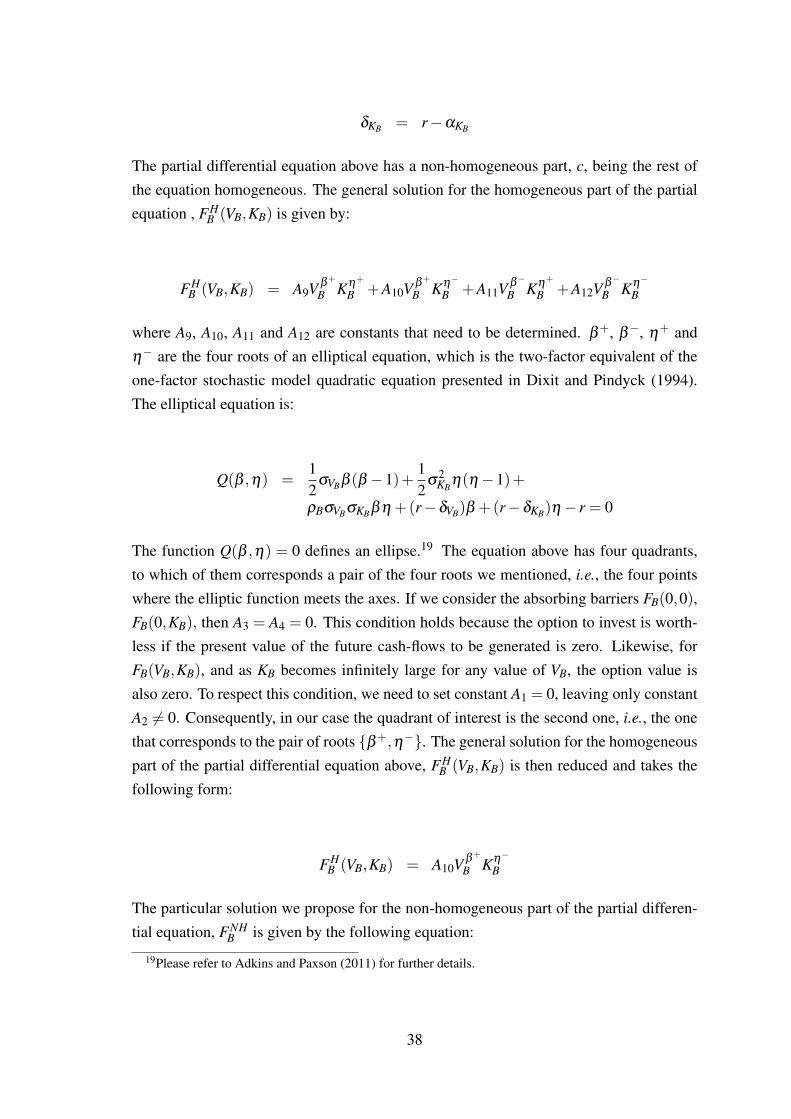
δKB = r−αKB

The partial differential equation above has a non-homogeneous part, c, being the rest ofthe equation homogeneous. The general solution for the homogeneous part of the partialequation , FH

B (VB,KB) is given by:

FHB (VB,KB) = A9V β+

B Kη+

B +A10V β+

B Kη−

B +A11V β−

B Kη+

B +A12V β−

B Kη−

B

where A9, A10, A11 and A12 are constants that need to be determined. β+, β−, η+ andη− are the four roots of an elliptical equation, which is the two-factor equivalent of theone-factor stochastic model quadratic equation presented in Dixit and Pindyck (1994).The elliptical equation is:

Q(β ,η) =12

σVBβ (β −1)+12

σ2KB

η(η−1)+

ρBσVBσKBβη +(r−δVB)β +(r−δKB)η− r = 0

The function Q(β ,η) = 0 defines an ellipse.19 The equation above has four quadrants,to which of them corresponds a pair of the four roots we mentioned, i.e., the four pointswhere the elliptic function meets the axes. If we consider the absorbing barriers FB(0,0),FB(0,KB), then A3 = A4 = 0. This condition holds because the option to invest is worth-less if the present value of the future cash-flows to be generated is zero. Likewise, forFB(VB,KB), and as KB becomes infinitely large for any value of VB, the option value isalso zero. To respect this condition, we need to set constant A1 = 0, leaving only constantA2 6= 0. Consequently, in our case the quadrant of interest is the second one, i.e., the onethat corresponds to the pair of roots {β+,η−}. The general solution for the homogeneouspart of the partial differential equation above, FH

B (VB,KB) is then reduced and takes thefollowing form:

FHB (VB,KB) = A10V β+

B Kη−

B

The particular solution we propose for the non-homogeneous part of the partial differen-tial equation, FNH

B is given by the following equation:

19Please refer to Adkins and Paxson (2011) for further details.

38

FNHB = −c

r

Joining the homogeneous and non-homogeneous solutions, we obtain the following ex-pression which satisfies the whole partial differential equation:

FHB (VB,KB)+FNH

B = FB(VB,KB) = A10V β+

B Kη−

B −cr

Hence, the value-matching condition will be given by:

FB(V ∗B ,K∗B) = A10V ∗

β+

B K∗η−

B − cr=V ∗B −K∗B

Since the value-matching condition above does not support homogeneity of degree one onboth sides (which means that β++ η− 6=1), we follow Adkins and Paxson (2011) solutionand construct a set of three simultaneous equations. The first equation is the ellipticalequation, presented above and reproduced below:

Q(β ,η) =12

σ2VB

β (β −1)+12

σ2KB

η(η−1)+

ρσVBσKBβη +(r−δVB)β +(r−δKB)η− r = 0

The other two equations are the two smooth-pasting conditions derived from the value-matching condition above. The first smooth-pasting condition is the first-order derivativeof the value-matching condition, in respect to V ∗B . After applying some rules of calculus,we reach the expression for the first smooth-pasting condition, which is given by thefollowing equation:

β+(V ∗B −K∗B +

cr) = V ∗B

The second smooth-pasting condition is the first-order derivative of the value matchingcondition, in respect to K∗B. Likewise, after applying some rules of calculus, we reach theexpression for the second smooth-pasting condition, given by the following equation:

39

η−(V ∗B −K∗B +

cr) = −K∗B

The set of simultaneous equations is thus formed by the elliptical equation and the twosmooth-pasting conditions. We need to set K∗B since we are in the presence of four uncer-tains (K∗B,V

∗B ,β

+,η−) and only have three equations available. Firstly, we solve the set ofsimultaneous equations considering that c= 0. This procedure enables us to obtain the se-lected bidder cash-flows trigger in the absence of a contractual penalty, which we denoteby V+

B . Secondly, we solve the same set of simultaneous equations to determine the exactvalue for c that moves V+

B downwards to perfectly meet the government cash-flows trig-ger, V ∗G. By repeating this process many times attributing different values for K∗B, we areable to define a discriminatory boundary separating the selected bidder investing regionfrom the selected bidder waiting region, formed by a set of countless pairs, {K∗B;V ∗B}.

The selected bidder should invest when both triggers, K∗B and V ∗B are simultaneously at-tained, i.e., {KB,VB} ≥ {K∗B,V ∗B}. When both triggers are simultaneously attained, thevalue of the option to invest equals the project’s expected net present value. Otherwise,the selected bidder should wait and defer the investment. Hence, the value of the selectedbidder investment opportunity is given by:

FB(VB,KB) =

(V ∗B −K∗B +cr )(

VBV ∗B

)β+ (KBK∗B

)η−

− cr ; i f {KB,VB}< {K∗B,V ∗B}

VB−KB ; i f {KB,VB} ≥ {K∗B,V ∗B}

Therefore, the value of the selected bidder option to invest in a project where a legalpenalty, c is enforced is given by the same function we presented when we derived thegovernment expectation about the private firm decision to invest, FP(VP,KP).

Figure 1 shows the selected bidder discriminatory boundary, assuming that the value ofthe legal penalty included in the contract is c2 = 1.9222. We consider values for K∗Branging from 80 to 480 and also consider that: σVB = 0.15; σKB = 0.10; ρB = 0; r = 0.05;δBV = δBK = 0.03; γ = 0.2.

40

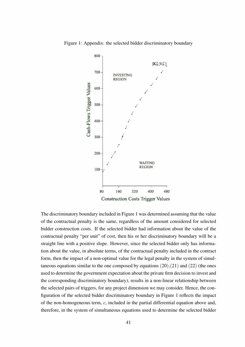
Figure 1: Appendix: the selected bidder discriminatory boundary

The discriminatory boundary included in Figure 1 was determined assuming that the valueof the contractual penalty is the same, regardless of the amount considered for selectedbidder construction costs. If the selected bidder had information about the value of thecontractual penalty “per unit” of cost, then his or her discriminatory boundary will be astraight line with a positive slope. However, since the selected bidder only has informa-tion about the value, in absolute terms, of the contractual penalty included in the contractform, then the impact of a non-optimal value for the legal penalty in the system of simul-taneous equations similar to the one composed by equations (20),(21) and (22) (the onesused to determine the government expectation about the private firm decision to invest andthe corresponding discriminatory boundary), results in a non-linear relationship betweenthe selected pairs of triggers, for any project dimension we may consider. Hence, the con-figuration of the selected bidder discriminatory boundary in Figure 1 reflects the impactof the non-homogeneous term, c, included in the partial differential equation above and,therefore, in the system of simultaneous equations used to determine the selected bidder

41

discriminatory boundary.

42

References

Adkins, R. and D. Paxson: (2011), ‘Renewing Assets with Uncertain Revenues and Operating

Costs’. Journal of Financial and Quantitative Analysis Vol. 46, Nº 3, 785–813.

Algarni, A. M., D. Arditi, and G. Polat: (2007), ‘Build-Operate-Transfer in Infrastructure Projects

in the United States’. Journal of Construction Engineering and Management Vol. 133, Nº 10,

728–735.

Alonso-Conde, A., C. Brown, and J. Rojo-Suarez: (2007), ‘Public-Private Partnerships: Incen-

tives, Risk Transfer and Real Options’. Review of Financial Economics Vol. 16, Nº 4, 335–349.

Armada, M. J. R., P. Pereira, and A. Rodrigues: (2013), ‘Optimal Investment with Two-Factor

Uncertainty’. Mathematics and Financial Economics Forthcoming.

Armada, M. J. R., P. J. Pereira, and A. Rodrigues: (2012), ‘Optimal Subsidies and Guarantees in

Public-Private Partnerships’. The European Journal of Finance Vol. 18, Nº 5, 469–495.

Brandao, L. E. and E. Saraiva: (2008), ‘The Option Value of Government Guarantees in Infras-

tructure Projects’. Construction Management and Economics Vol. 26, Nº 11, 1171–1180.

Caselli, S., S. Gatii, and A. Marciante: (2009), ‘Pricing Final Indemnification Payments to Pri-

vate Sponsors in Project-Financed Public-Private Partnerships: An Application of Real Options

Valuation’. Journal of Applied Corporate Finance Vol. 21, Nº 3, 95–106.

Cheah, C. and J. Liu: (2006), ‘Valuing Governmental Support in Infrastructure Projects as Real

Options Using Monte Carlo Simulation’. Construction Management and Economics Vol. 24,Nº 5, 515–54.

Chiara, N., M. J. Garvin, and J. Vecer: (2007), ‘Valuing Simple Multiple-Exercise Real Options

in Infrastructure Projects’. Journal of Infrastructure Systems Vol. 13, Nº 2, 97–104.

Coase, R. H.: (1960), ‘The Problem of Social Cost’. Journal of Law and Economics Vol. 3, Nº 1,

1–44.

Constantinides, G.: (1978), ‘Market Risk Adjustment in Project Valuation’. Journal of Finance

Vol. 33, Nº 2, 603–616.

Dixit, A. and R. Pindyck: (1994), Investment Under Uncertainty. New Jersey: Princeton Univer-

sity Press.

Ferreira, D. and K. Khatami: (1996), ‘Financing Private Infrastructure in Developing Countries’.

World Bank - Discussion Papers 343, 1–32.

43

Ho, S. P. and L. Y. Liu: (2002), ‘An Option Pricing-Based Model for Evaluating the Financial

Viability of Privatized Infrastructure Projects’. Construction Management and Economics Vol.20, Nº 2, 143–156.

Huang, Y. and S. Chou: (2006), ‘Valuation of the Minimum Revenue Guarantee and the Option to

Abandon in BOT Infrastructure Projects’. Construction Management and Economics Vol. 24,Nº 4, 379–389.

Huang, Y.-L. and C.-C. Pi: (2009), ‘Valuation of Multi-Stage BOT Projects Involving Dedicated

Asset Investments: A Sequential Compound Option Approach’. Construction Management and

Economics Vol. 27, Nº 7, 653–666.

Kwak, Y. H., Y. Y. Chih, and C. W. Ibbs: (2009), ‘Towards a Comprehensive Understanding of

Public Private Partnerships for Infrastructure Development’. California Management Review

Vol. 51, Nº 2, 51–78.

Liu, J. and C. Y. J. Cheah: (2009), ‘Real Option Application in PPP/PFI Project Negotiation’.

Construction Management and Economics Vol. 27, Nº 4, 331–342.

Maskin, E. and J. Tirole: (2008), ‘Public-Private Partnerships and Government Spending Limits’.

International Journal of Industrial Organization Vol. 26, Nº 2, 412–420.

McDonald, R. and D. Siegel: (1986), ‘The Value of Waiting to Invest’. The Quarterly Journal of

Economics Vol. 101, Nº 4, 707–728.

Paxson, D. and H. Pinto: (2005), ‘Rivalry under Price and Quantity Uncertainty’. Review of

Financial Economics Vol. 14, Nº 3-4, 209–224.

Pereira, P., A. Rodrigues, and M. R. Armada: (2006), ‘The Optimal Timing for the Construction

of an International Airport: a Real Options Approach with Multiple Stochastic Factors and

Shocks’. 10th Real Options Conference, NewYork. pp. 1–20.

Rus, G. and G. Nombela: (2007), ‘Is Investment in High Speed Rail Socially Profitable?’. Journal

of Transport Economics and Policy Vol. 41, Nº 1, 3–23.

Shan, L., M. Garvin, and R. Kumar: (2010), ‘Collar Options to Manage Revenue Risks in Real

Toll Public-Private Partnership Transport Projects’. Construction Management and Economics

Vol. 28, Nº 10, 1057–1059.

Shen, L. and Y. Z. Wu: (2005), ‘Risk Concession Model for Build-Operate-Transfer Contract

Projects’. Journal of Construction Engineering and Management Vol. 131, Nº 2, 211–220.

Shen, L. Y., H. LI, and Q. M. Li: (2002), ‘Alternative Concession Model for Build Operate Trans-

fer Contract Projects’. Journal of Construction Engineering and Management Vol.128, Nº 4,

326–330.

44

Trigeorgis, L.: (1996), Real Options: Managerial Flexibility and Strategy in Resource Allocation.

Boston: MIT Press.

Zhang, X. Q. and M. M. Kumaraswamy: (2001), ‘Procurement Protocols for Public-Private Part-

nered Projects’. Journal of Construction Engineering and Management Vol. 127, Nº 5, 351–

358.

45