visual media processing using matlab beginner's guide

Visual Media Processing Using MATLAB Beginner's Guide

George Siogkas

Chapter No. 3 "Morphological Operations and

Object Analysis"

In this package, you will find: A Biography of the author of the book

A preview chapter from the book, Chapter NO.3 "Morphological Operations and Object Analysis"

A synopsis of the book’s content

Information on where to buy this book

About the Author George Siogkas is currently the Associate Dean of the Department of Engineering and Informatics at New York College, Greece, where he has been teaching as a senior lecturer for the past four years. He also has more than ten years of research experience in the academia. His keen passion for MATLAB programming, especially in the areas of image and video processing, was developed while working towards a PhD in the field of computer vision for intelligent transportation systems.

Dr. Siogkas received his PhD in Electrical and Computer Engineering from the University of Patras, Greece in 2013.

For more information about the author, visit his webpage, at http://www.cvrlab.com/gsiogkas.

For More Information: www.packtpub.com/visual-media-processing-using-matlab-beginners-

guide/book

http://www.packtpub.com/visual-media-processing-using-matlab-beginners-guide/book

I would like to first and foremost thank my beautiful wife, Maro, who put up with my exhausting writing schedule for both this book and my PhD thesis, while staying focused enough to organize our wedding. I would also like to thank my parents and my brother for their continuous support, especially during this past year. Without the encouragement from all of them, this project would never even have got started in the first place.

I would also like to thank everyone at Packt Publishing who got involved in this book, especially Joanne Fitzpatrick, Hardik Patel, Navu Dhillon, and Anila Vincent. They played a very important role in helping me understand the rationale behind such a writing project and provided invaluable feedback throughout the writing process. Also, a special thanks goes to the reviewers, R. Surya Murali, Ashish Uthama, and Alexander Wright, who provided very useful and insightful comments and suggestions for improving the quality of the book. Without them all, this book would never have reached its publishing stage.


guide/book


Visual Media Processing Using MATLAB Beginner's Guide Digital visual media has, undoubtedly, become a vital part of our everyday lives. Analog means of storing and processing information have gradually faded and are nowadays used either by aficionados of analog media, or for very specialized applications. Capturing and storing image or video information have rapidly become common, fast, and cheap processes, since almost everyone can have access to a digital electronic device that can be used for these aims, whether it is a photographic or video camera, or even a mobile phone. The outburst of visual media-capturing devices has led to an increase of amateur photographers and weekend filmmakers, who oft en have a problem deciding what soft ware to use to process their stored images or videos. The rule of thumb is that free soft ware solutions oft en have limited functionalities or are very complicated, while commercial solutions tend to be very expensive and sometimes do not provide all the functionalities that a user would hope for.

This book presents a rather uncommon alternative solution that might not be considered by users who only need an image, or a video editing soft ware, but could certainly appeal to users who are also students, scientists, or just have easy access to the multi functional, high level programming environment, called MATLAB.

What This Book Covers Chapter 1, Basic Image Manipulations, introduces you to the environment of MATLAB and takes you on a tour to its basic tools and functionalities. Then, image importing and displaying in MATLAB is discussed, followed by a demonstration of the MATLAB GUI for image manipulation. Basic image transformations are covered, such as rotating/flipping, resizing, and cropping an image. Finally, different ways of writing an image are presented. The chapter includes hands-on examples that tie most of the processes covered, together.

Chapter 2, Working with Pixels in Grayscale Images, is based on examples of pixel-based processing of an image. Several classic processes for image enhancement are discussed, such as thresholding, local, or global contrast enhancement. The methods presented use several techniques that gently introduce you to the secrets of MATLAB programming. A practical example in image enhancement concludes this chapter.


guide/book


Chapter 3, Morphological Operations and Object Analysis, introduces the basic methods of morphological image analysis. In it, you will learn of ways to perform binarization of a grayscale image using the thresholding methods. Edge detection and other morphological operators are presented and explained, so that you learn how to select and manipulate particular image regions that interest you the most. You will also learn the techniques that automatically detect corners, circles, and lines in an image. Several hands-on examples will vividly demonstrate all these techniques.

Chapter 4, Working with Color Images, extends previous methods to color images. Some of the processes mentioned for grayscale are now revisited for color image processing. Different color spaces and their advantages are explained with examples on color enhancement in MATLAB. You will learn how illuminati on and color can be separated and processed independently. The technique for color isolation is explained through a practical example and finally, some of the methods mentioned previously are used to teach you how to develop a popular application: red eye correction in your photographs.

Chapter 5, 2-Dimensional Image Filtering, dives into some more complex issues for image filtering, such as deblurring and sharpening of images. You will get to work on more sophisticated techniques for image denoising. Some more interesting and fun examples will let you start enjoying your experience more deeply. We will work on ways to apply some of the filter locally, to enhance or blur specific image regions.

Chapter 6, Mixing Images for Science or Art, will wake up the artist, or the scientist in you. You will learn the techniques that mix channels of multi spectral images for scientific visualization. Then, we will present fun, hands-on examples for blending, or stitching images, to produce artistic results. We will also work on ways to create artistic HDR (High Dynamic Range) images in MATLAB. Finally, we will present a simple way to create panoramic images.

Chapter 7, Adding Motion – From Static Images to Digital Videos, introduces you to video processing by building on the previous knowledge you have acquired. The fact, that videos can be generated by static images, will help you to better comprehend basic ideas. So, after covering the basics of video frame processing in MATLAB and demonstrating how we can load and play back videos, we will show how to create a video from static images. The construction of a time-lapse video is the basic hands-on example we will be working on in this chapter.


guide/book


Chapter 8, Acquiring and Processing Videos, demonstrates the functionalities of the image acquisition tool for MATLAB. You will be given step-by-step examples on ways to shoot video with your camera and use your computer as a Digital Video Recorder, using the special GUI tool contained in MATLAB. Video compression and basic color video processing techniques are also demonstrated in this chapter, accompanied by a discussion on performance issues.

Chapter 9, Spatiotemporal Video Processing, introduces you to command line manipulation and processing of videos. After covering basic video frames manipulations in MATLAB, you will learn how to deinterlace videos, using intra-frame, inter-frame, or mixed techniques. Furthermore, spatiotemporal video filtering is presented, with hands-on examples to help you get the idea.

Chapter 10, From Beginner to Expert – Handling Motion and 3-D, introduces you to methods of motion detection in videos. Building on basic knowledge, we will get to the point of creating a simple surveillance system in MATLAB. You will also be taught the basics of estimating motion using popular optical flow algorithms, included in one of the toolboxes of MATLAB. You will also be introduced to feature-based image registration for motion compensation. The working example for this will be video stabilization. Finally, we will introduce an example of three-dimensional video and cover a very basic and fun example of turning a regular video to a 3-D one.


guide/book


Morphological Operations and Object Analysis

In the previous chapters, you learned various image processing techniques related to image manipulation. In some of them, we concentrated our processing on specific regions of the images, predefined by the user. However, many processes that involve visual media enhancement need to focus on automatically specified regions of interest. In this chapter, we will present some basic techniques for selecting the regions of interest, based on image morphology. We will also revisit the manual selection of regions, presenting some more flexible tools. Then, you will be demonstrated some basic object analysis techniques such as edge, corner, and circle detection. Several examples will help you better understand how morphological operations combined with object analysis methods can help in targeting our processing on specific areas of an image.

In this chapter, we shall:

Learn about binary images and how they are used for masking

Learn about morphological operati ons and their importance

Learn how to use MATLAB tools for Region Of Interest (ROI) selecti on

Learn how to detect edges, corners, and circles in an image

So, let's start!

3


guide/book


Morphological Operati ons and Object Analysis

[ 64 ]

The importance of binary imagesTo understand the noti on of morphological operati ons , we will have to revisit the thresholding techniques presented in the previous chapter. We have already menti oned that thresholding an image leads to binary images, which are defi ned by their two possible pixel values; 0 (for black) and 1 (for white). The way to convert a grayscale image to binary is through thresholding; that is, setti ng the pixels above a certain value to 1 and the rest to 0. Let's now explain the basic reasons for binarizing an image. The purpose of image binarizati on can be split into two levels. At a fi rst level, it is used to pinpoint the pixels of an image that interest us (usually called regions of interest or simply, ROIs), thus giving us a quick and easy overview of the image content. The binary images derived, are oft en called masks . At a second level, it can be used for processing only the selected ROIs (with pixel values equal to 1) defi ned by the mask, leaving the rest of the image unaff ected. Let's see the diff erence using, an example that covers both the functi onaliti es.

Time for action – understanding the value of thresholdingIn this example, we will try to separate the two useful aspects of image binarizati on, so that we can then use them appropriately. The fi rst thing we will do is to locate a faulty ROI of an image and then we will try to cover it using what we have already learned. For this example, we will be again using my great-grandmother's photograph. So, let's start:

1. First, we need to load the grayscale image we have created in the previous chapter, by using imread:

>> img = imread('graygrandma.BMP');

2. The second step is to perform thresholding, as we have already done in the previous chapter (using the same threshold, which was 220):

>> img_bin = (img> 220); % Image img_bin is now binary

3. Now, let's perform some rough patching of the image in the specifi c ROI that has pixels with values over 220. A way to accomplish this is to change these values to a grayer shade, for example, 100:

>> img_patched = img;>> img_patched(img_bin) = 100;

4. At this point, we have three images in our Workspace. The original one (img), the binarized one (img_bin) and the patched one (img_patched). Let's display them side-by-side to get a bett er understanding of what happened:

>> subplot(1,3,1),imshow(img),title('Original Image')>> subplot(1,3,2),imshow(img_bin),title('Binarized Image')>> subplot(1,3,3),imshow(img_patched),title('Patched Image')


guide/book


Chapter 3

[ 65 ]

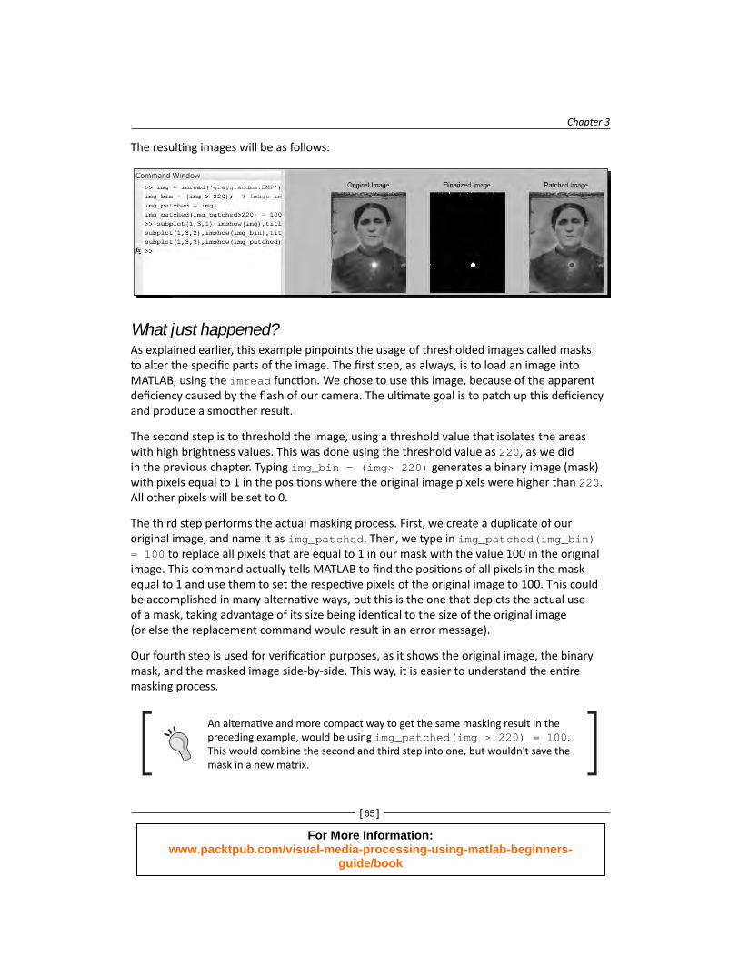
The resulti ng images will be as follows:

What just happened?As explained earlier, this example pinpoints the usage of thresholded images called masks to alter the specifi c parts of the image. The fi rst step, as always, is to load an image into MATLAB, using the imread functi on . We chose to use this image, because of the apparent defi ciency caused by the fl ash of our camera. The ulti mate goal is to patch up this defi ciency and produce a smoother result.

The second step is to threshold the image, using a threshold value that isolates the areas with high brightness values. This was done using the threshold value as 220, as we did in the previous chapter. Typing img_bin = (img> 220) generates a binary image (mask) with pixels equal to 1 in the positi ons where the original image pixels were higher than 220. All other pixels will be set to 0.

The third step performs the actual masking process. First, we create a duplicate of our original image, and name it as img_patched. Then, we type in img_patched(img_bin) = 100 to replace all pixels that are equal to 1 in our mask with the value 100 in the original image. This command actually tells MATLAB to fi nd the positi ons of all pixels in the mask equal to 1 and use them to set the respecti ve pixels of the original image to 100. This could be accomplished in many alternati ve ways, but this is the one that depicts the actual use of a mask, taking advantage of its size being identi cal to the size of the original image (or else the replacement command would result in an error message).

Our fourth step is used for verifi cati on purposes, as it shows the original image, the binary mask, and the masked image side-by-side. This way, it is easier to understand the enti re masking process.

An alternati ve and more compact way to get the same masking result in the preceding example, would be using img_patched(img > 220) = 100. This would combine the second and third step into one, but wouldn't save the mask in a new matrix.


guide/book



[ 66 ]

The preceding example describes a very useful technique in its simplest form. This simple procedure has two serious fl aws; one in the mask defi niti on and one in the image masking process.

The fl aw in the mask defi niti on is the diffi culty in pinpointi ng the specifi c ROI of our choice, using just the pixel values. Rarely can we isolate the region we need, by setti ng a specifi c threshold. Even in the example we saw (which is almost ideal for this simple technique), the mask derived from thresholding includes some pixels equal to 1 in other areas (for example, the frame of the picture). Also, the image masking result reveals that the area selected is a litt le smaller than it should be.

The fl aw in the masking process is that the result is roughly patched up and just covers the area with brightness values that are closer to what would be expected. However, the ideal result would replace the bright area with something more complex than a patch of equal brightness values. This patch could be a part of an image that more closely resembles what has been destroyed by the fl ash.

In the rest of the chapter, we will be focusing on ways to refi ne the mask selecti on process, so that the resulti ng mask is more suitable to our needs. This will be accomplished using various morphological operati ons that will tweak our mask.

Enlarging and shrinking a region of interestA very common technique for refi ning a region of interest derived using thresholding is either enlarging or shrinking it to fi t our target size. This can be accomplished by the morphological operati ons called dilati on and erosion , respecti vely. These operati ons can be implemented in MATLAB using their respecti ve functi ons, intuiti vely named imdilate and imerode.

Explaining and analyzing the mathemati cal properti es of dilati on and erosion lie beyond the scope of this book. We will instead explain their signifi cance using practi cal examples that demonstrate their importance for image processing. The basic idea that you have to understand before we start, is that the two operati ons can be used for enlarging or shrinking an ROI (denoted by the instances of 1 in the image) using a structuring element. Structuring elements can be small binary images generated by the user either arbitrarily (placing the instances of 1 and 0 in a small image), or by using the strel functi on. The choice of a structuring element should be made following two simple rules:

The larger the structuring element, the larger the enlarging/shrinking factor

Using a structuring element more similar to the shape of the ROI will typically give you a bett er result

Let's dive right in, to understand the physical meaning of all these concepts in practi ce.


guide/book


Chapter 3

[ 67 ]

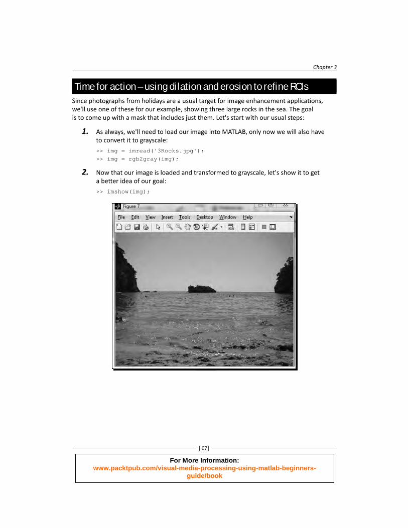
Time for action – using dilation and erosion to refi ne ROIsSince photographs from holidays are a usual target for image enhancement applicati ons, we'll use one of these for our example, showing three large rocks in the sea. The goal is to come up with a mask that includes just them. Let's start with our usual steps:

1. As always, we'll need to load our image into MATLAB, only now we will also have to convert it to grayscale:

>> img = imread('3Rocks.jpg');>> img = rgb2gray(img);

2. Now that our image is loaded and transformed to grayscale, let's show it to get a bett er idea of our goal:

>> imshow(img);


guide/book



[ 68 ]

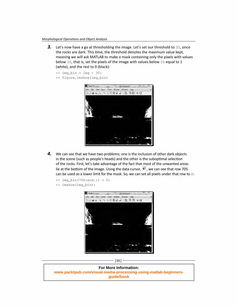
3. Let's now have a go at thresholding the image. Let's set our threshold to 30, since the rocks are dark. This ti me, the threshold denotes the maximum value kept, meaning we will ask MATLAB to make a mask containing only the pixels with values below 30, that is, set the pixels of the image with values below 30 equal to 1 (white), and the rest to 0 (black):

>> img_bin = img < 30;>> figure,imshow(img_bin)

4. We can see that we have two problems; one is the inclusion of other dark objects in the scene (such as people's heads) and the other is the subopti mal selecti on of the rocks. First, let's take advantage of the fact that most of the unwanted areas lie at the bott om of the image. Using the data cursor, , we can see that row 705 can be used as a lower limit for the mask. So, we can set all pixels under that row to 0:

>> img_bin(706:end,:) = 0;>> imshow(img_bin);


guide/book


Chapter 3

[ 69 ]

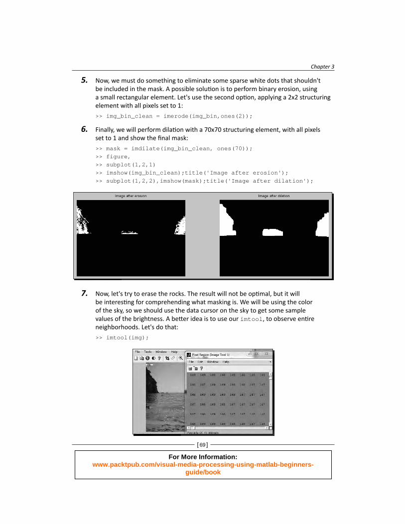
5. Now, we must do something to eliminate some sparse white dots that shouldn't be included in the mask. A possible soluti on is to perform binary erosion, using a small rectangular element. Let's use the second opti on, applying a 2x2 structuring element with all pixels set to 1:

>> img_bin_clean = imerode(img_bin,ones(2));

6. Finally, we will perform dilati on with a 70x70 structuring element, with all pixels set to 1 and show the fi nal mask:

>> mask = imdilate(img_bin_clean, ones(70));>> figure,>> subplot(1,2,1)>> imshow(img_bin_clean);title('Image after erosion');>> subplot(1,2,2),imshow(mask);title('Image after dilation');

7. Now, let's try to erase the rocks. The result will not be opti mal, but it will be interesti ng for comprehending what masking is. We will be using the color of the sky, so we should use the data cursor on the sky to get some sample values of the brightness. A bett er idea is to use our imtool, to observe enti re neighborhoods. Let's do that:

>> imtool(img);


guide/book



[ 70 ]

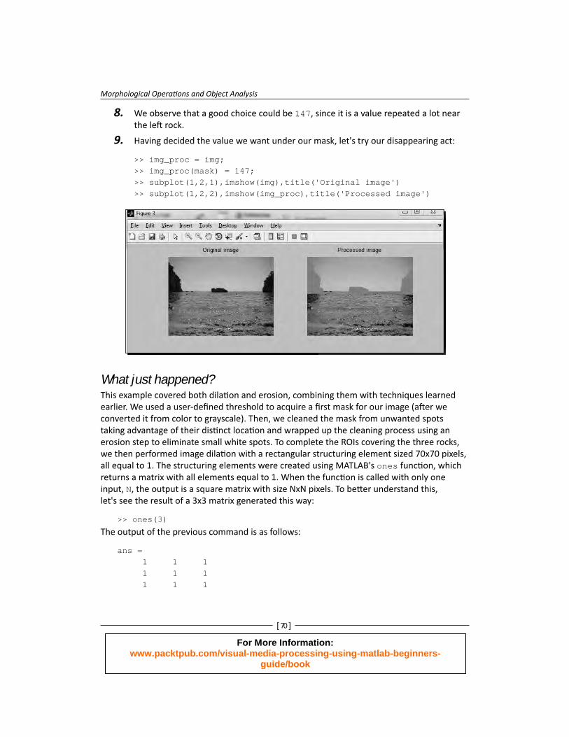
8. We observe that a good choice could be 147, since it is a value repeated a lot near the left rock.

9. Having decided the value we want under our mask, let's try our disappearing act:

>> img_proc = img;>> img_proc(mask) = 147;>> subplot(1,2,1),imshow(img),title('Original image')>> subplot(1,2,2),imshow(img_proc),title('Processed image')

What just happened?This example covered both dilati on and erosion, combining them with techniques learned earlier. We used a user-defi ned threshold to acquire a fi rst mask for our image (aft er we converted it from color to grayscale). Then, we cleaned the mask from unwanted spots taking advantage of their disti nct locati on and wrapped up the cleaning process using an erosion step to eliminate small white spots. To complete the ROIs covering the three rocks, we then performed image dilati on with a rectangular structuring element sized 70x70 pixels, all equal to 1. The structuring elements were created using MATLAB's ones functi on, which returns a matrix with all elements equal to 1. When the functi on is called with only one input, N, the output is a square matrix with size NxN pixels. To bett er understand this, let's see the result of a 3x3 matrix generated this way:

>> ones(3)

The output of the previous command is as follows:

ans = 1 1 1 1 1 1 1 1 1


guide/book


Chapter 3

[ 71 ]

Aft er creati ng our mask, we applied a patching-up process like the one described in the previous secti on. This ti me, our goal was to erase the rocks from the picture, replacing their pixels' values with one that is descripti ve of the sky. Of course, using just one brightness value for such big areas, ends up with a fl at result, which is less subtle than we would like. However, the main goal of erasing the rocks was achieved to a good extent.

The use of imerode to eliminate small objects from our mask is not always a good idea, since it aff ects all binary objects in the image. For this example, we used it in conjuncti on with imdilate. A bett er choice for such tasks would be to use the bwareaopen functi on, which eliminates small objects of a predefi ned size from the image. In the preceding example, to eliminate objects smaller than 6 pixels, we would replace the step img_bin_clean = imerode(img_bin, ones(2)); with img_bin_clean = bwareaopen(img_bin, 6);.

Choosing a structuring elementWe menti oned earlier the usage of structuring elements and the two rules we must follow when choosing them. However, in our example of dilati on and erosion, we used a rather simple rectangular structuring element, consisti ng of instances of 1. Is there a bett er choice? The answer is yes. The objects we want to mask are not rectangular, so the best choice is defi nitely not a rectangular structuring element. However, we can observe that the three rocks are not similar. The two rocks at the sides could be thought of as similar, but they have opposite orientati ons (that is, they look like they are mirrored). The shape of the small rock in the middle does not resemble the others. All these facts lead us to the conclusion that more than one structuring element should be used. However, we fall right into the next problem; how will we use diff erent structuring elements for diff erent areas? For this, we will recollect a technique we used in the previous chapter.

But fi rst thing fi rst; we should start with choosing the ideal structuring element for each rock. As you may already have understood from the results of the previous example, the sides of the rocks that are att ached to the left and right image borders remain almost untouched. Their only alterati on aft er imdilate. is being expanded at the top and bott om. The middle rock has expanded in all directi ons aft er dilati on.


guide/book



[ 72 ]

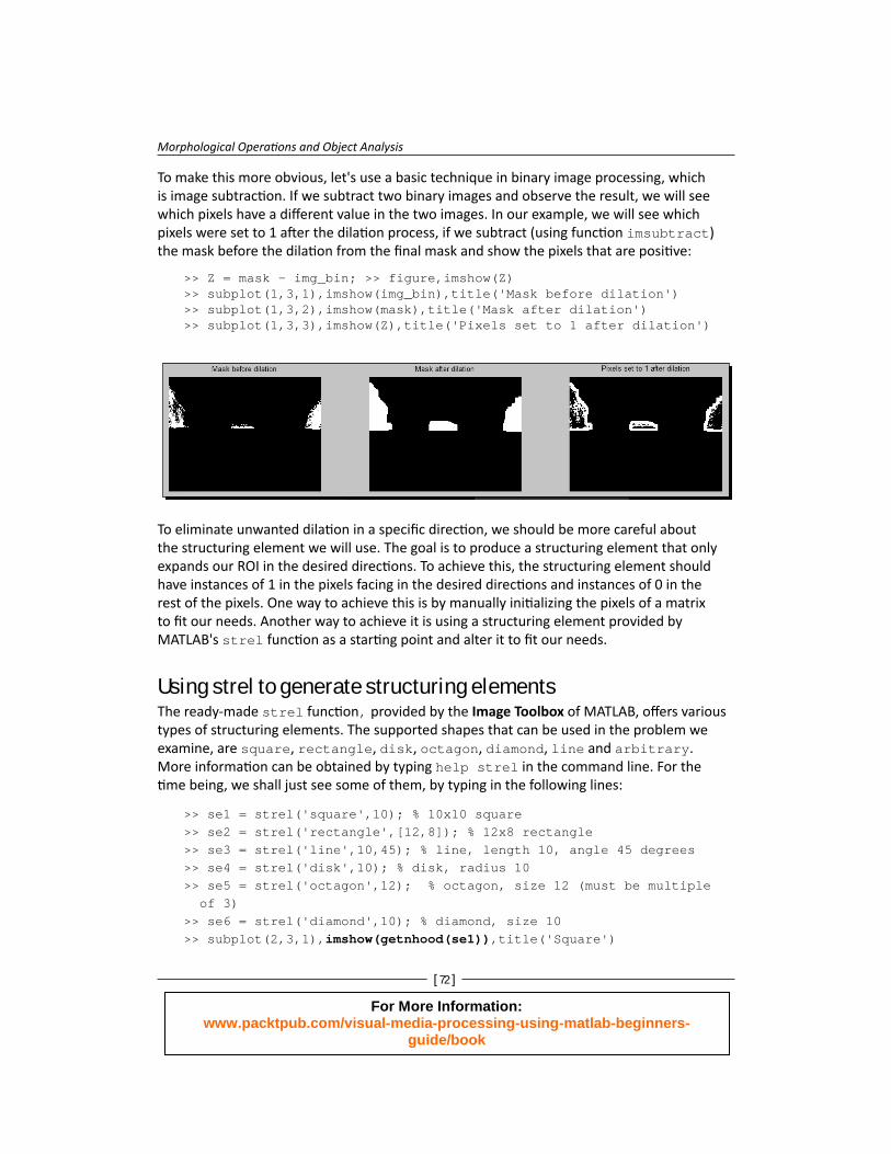
To make this more obvious, let's use a basic technique in binary image processing, which is image subtracti on. If we subtract two binary images and observe the result, we will see which pixels have a diff erent value in the two images. In our example, we will see which pixels were set to 1 aft er the dilati on process, if we subtract (using functi on imsubtract) the mask before the dilati on from the fi nal mask and show the pixels that are positi ve:

>> Z = mask - img_bin; >> figure,imshow(Z)>> subplot(1,3,1),imshow(img_bin),title('Mask before dilation')>> subplot(1,3,2),imshow(mask),title('Mask after dilation')>> subplot(1,3,3),imshow(Z),title('Pixels set to 1 after dilation')

To eliminate unwanted dilati on in a specifi c directi on, we should be more careful about the structuring element we will use. The goal is to produce a structuring element that only expands our ROI in the desired directi ons. To achieve this, the structuring element should have instances of 1 in the pixels facing in the desired directi ons and instances of 0 in the rest of the pixels. One way to achieve this is by manually initi alizing the pixels of a matrix to fi t our needs. Another way to achieve it is using a structuring element provided by MATLAB's strel functi on as a starti ng point and alter it to fi t our needs.

Using strel to generate structuring elementsThe ready-made strel functi on, provided by the Image Toolbox of MATLAB, off ers various types of structuring elements. The supported shapes that can be used in the problem we examine, are square, rectangle, disk, octagon, diamond, line and arbitrary. More informati on can be obtained by typing help strel in the command line. For the ti me being, we shall just see some of them, by typing in the following lines:

>> se1 = strel('square',10); % 10x10 square>> se2 = strel('rectangle',[12,8]); % 12x8 rectangle>> se3 = strel('line',10,45); % line, length 10, angle 45 degrees>> se4 = strel('disk',10); % disk, radius 10>> se5 = strel('octagon',12); % octagon, size 12 (must be multiple of 3)>> se6 = strel('diamond',10); % diamond, size 10>> subplot(2,3,1),imshow(getnhood(se1)),title('Square')


guide/book


Chapter 3

[ 73 ]

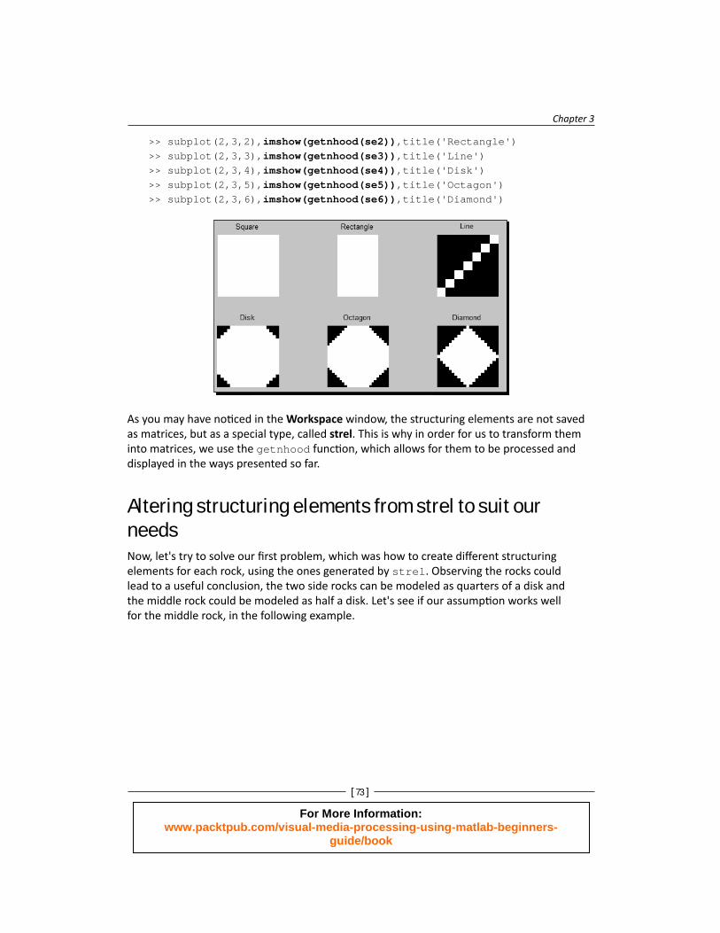
>> subplot(2,3,2),imshow(getnhood(se2)),title('Rectangle')>> subplot(2,3,3),imshow(getnhood(se3)),title('Line')>> subplot(2,3,4),imshow(getnhood(se4)),title('Disk')>> subplot(2,3,5),imshow(getnhood(se5)),title('Octagon')>> subplot(2,3,6),imshow(getnhood(se6)),title('Diamond')

As you may have noti ced in the Workspace window, the structuring elements are not saved as matrices, but as a special type, called strel. This is why in order for us to transform them into matrices, we use the getnhood functi on , which allows for them to be processed and displayed in the ways presented so far.

Altering structuring elements from strel to suit our needsNow, let's try to solve our fi rst problem, which was how to create diff erent structuring elements for each rock, using the ones generated by strel. Observing the rocks could lead to a useful conclusion, the two side rocks can be modeled as quarters of a disk and the middle rock could be modeled as half a disk. Let's see if our assumpti on works well for the middle rock, in the following example.


guide/book



[ 74 ]

Time for action – ROI refi nement using strelIn this example, we shall see how to use the disk structuring element from strel, to have a bett er masking result for the middle rock of our holiday picture. To focus on our task, we will fi rst crop the area we are mostly interested in. Assuming we have cleared our workspace using clear all (MATLAB's command to clear all the variables), we follow these steps:

1. Read our colored image, convert it to grayscale, and crop the area containing the middle rock:

>> img = imread('3rocks.jpg');>> rock = imcrop(rgb2gray(img));

2. Threshold the cropped image using the same threshold as before (30) and show the result side-by-side with the original:

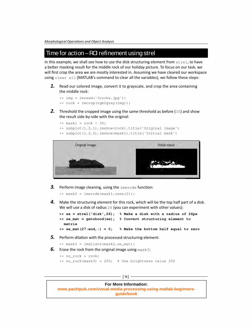
>> mask1 = rock < 30;>> subplot(1,2,1),imshow(rock),title('Original image')>> subplot(1,2,2),imshow(mask1),title('Initial mask')

3. Perform image cleaning, using the imerode functi on:

>> mask2 = imerode(mask1,ones(2));

4. Make the structuring element for this rock, which will be the top half part of a disk. We will use a disk of radius 26 (you can experiment with other values):

>> se = strel('disk',26); % Make a disk with a radius of 26px>> se_mat = getnhood(se); % Convert structuring element to

matrix>> se_mat(27:end,:) = 0; % Make the bottom half equal to zero

5. Perform dilati on with the processed structuring element:

>> mask3 = imdilate(mask2,se_mat);

6. Erase the rock from the original image using mask3:

>> no_rock = rock;>> no_rock(mask3) = 200; % Use brightness value 200


guide/book


Chapter 3

[ 75 ]

7. Demonstrate the results:

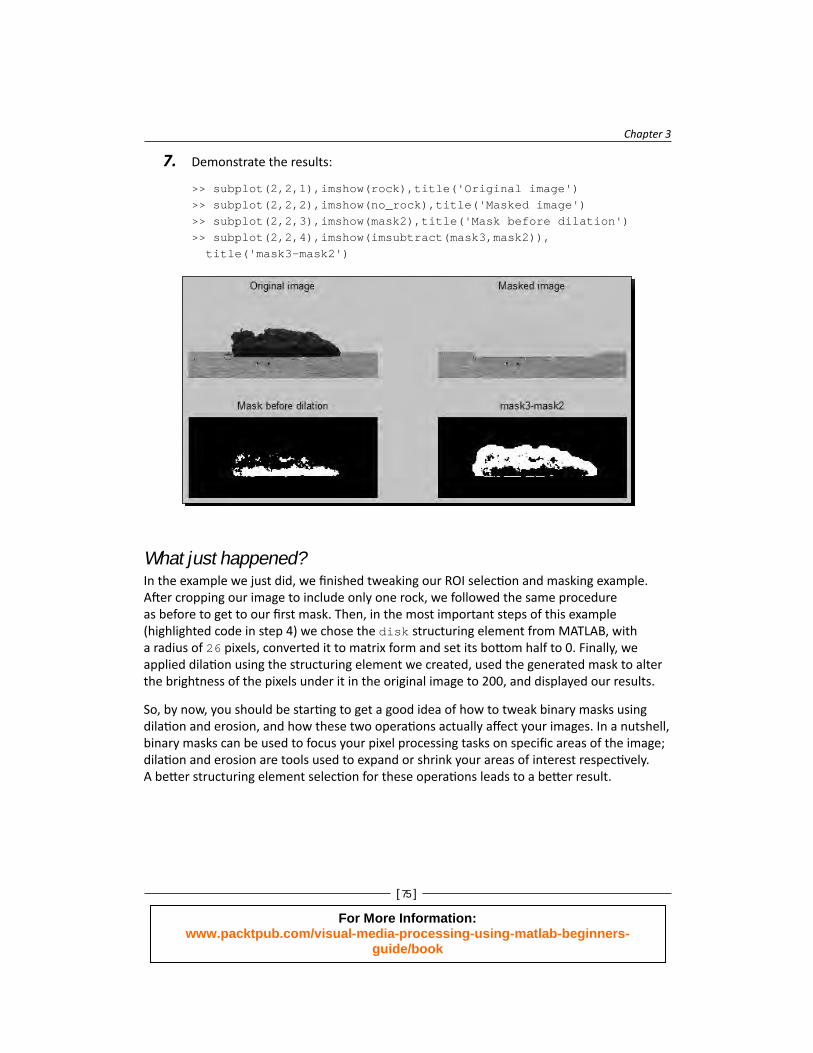
>> subplot(2,2,1),imshow(rock),title('Original image')>> subplot(2,2,2),imshow(no_rock),title('Masked image')>> subplot(2,2,3),imshow(mask2),title('Mask before dilation')>> subplot(2,2,4),imshow(imsubtract(mask3,mask2)), title('mask3-mask2')

What just happened?In the example we just did, we fi nished tweaking our ROI selecti on and masking example. Aft er cropping our image to include only one rock, we followed the same procedure as before to get to our fi rst mask. Then, in the most important steps of this example (highlighted code in step 4) we chose the disk structuring element from MATLAB, with a radius of 26 pixels, converted it to matrix form and set its bott om half to 0. Finally, we applied dilati on using the structuring element we created, used the generated mask to alter the brightness of the pixels under it in the original image to 200, and displayed our results.

So, by now, you should be starti ng to get a good idea of how to tweak binary masks using dilati on and erosion, and how these two operati ons actually aff ect your images. In a nutshell, binary masks can be used to focus your pixel processing tasks on specifi c areas of the image; dilati on and erosion are tools used to expand or shrink your areas of interest respecti vely. A bett er structuring element selecti on for these operati ons leads to a bett er result.


guide/book



[ 76 ]

Have a go hero – write a function to for local dilation/erosion

In the previous chapter, we saw how to write a functi on that performs enhancement of a rectangular area specifi ed by the user. Can you do the same for dilati on and erosion? The functi on should get three inputs; the original binary image, the structuring element and the selecti on of operati on (one for erosion and two for dilati on).

Well, the implementati on shouldn't seem so hard now. We will more or less base our functi on on what we did in the previous chapter. The fi rst step is to let the user crop the part of the image to be processed and save its coordinates. Then, we should switch to the specifi ed operati on based on the user's input. The selected operati on will then be performed on the original binary image using the structuring element provided as input. The fi nal step is to place the cropped region back on the image and return the output.

The functi on you should write, named CroppedDilationErosion.m , is defi ned as follows:

function [output] = CroppedDilationErosion(input,se,method)

% Function that performs area-based dilation or erosion with =% a user-defined structuring element.% Inputs:% input - Input image% se – Structuring element% method – Morphology operation (1: dilation, 2: erosion)% Output:% output - Output image (dilated or eroded)

To check if your functi on works as expected, you can use the mask from the previous example:

>> img = imread('3rocks.jpg');>> rock = rgb2gray(img);>> mask = rock < 30;>> mask2 = CroppedDilationErosion(mask,ones(10),2); % Erode mask>> mask3 = CroppedDilationErosion(mask,ones(10),1); % Dilate mask


guide/book


Chapter 3

[ 77 ]

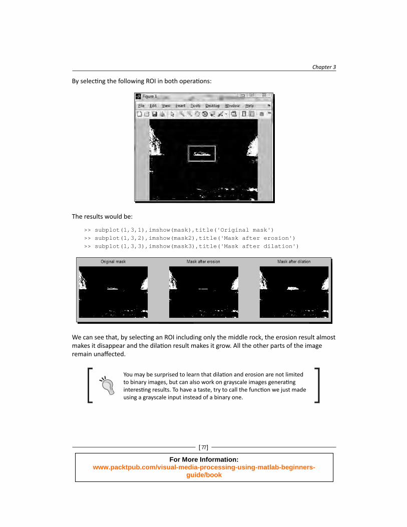
By selecti ng the following ROI in both operati ons:

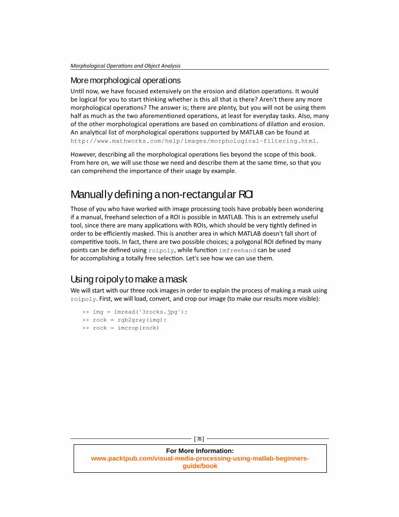
The results would be:

>> subplot(1,3,1),imshow(mask),title('Original mask')>> subplot(1,3,2),imshow(mask2),title('Mask after erosion')>> subplot(1,3,3),imshow(mask3),title('Mask after dilation')

We can see that, by selecti ng an ROI including only the middle rock, the erosion result almost makes it disappear and the dilati on result makes it grow. All the other parts of the image remain unaff ected.

You may be surprised to learn that dilati on and erosion are not limited to binary images, but can also work on grayscale images generati ng interesti ng results. To have a taste, try to call the functi on we just made using a grayscale input instead of a binary one.


guide/book



[ 78 ]

More morphological operationsUnti l now, we have focused extensively on the erosion and dilati on operati ons. It would be logical for you to start thinking whether is this all that is there? Aren't there any more morphological operati ons? The answer is; there are plenty, but you will not be using them half as much as the two aforementi oned operati ons, at least for everyday tasks. Also, many of the other morphological operati ons are based on combinati ons of dilati on and erosion. An analyti cal list of morphological operati ons supported by MATLAB can be found at http://www.mathworks.com/help/images/morphological-filtering.html.

However, describing all the morphological operati ons lies beyond the scope of this book. From here on, we will use those we need and describe them at the same ti me, so that you can comprehend the importance of their usage by example.

Manually defi ning a non-rectangular ROIThose of you who have worked with image processing tools have probably been wondering if a manual, freehand selecti on of a ROI is possible in MATLAB. This is an extremely useful tool, since there are many applicati ons with ROIs, which should be very ti ghtly defi ned in order to be effi ciently masked. This is another area in which MATLAB doesn't fall short of competi ti ve tools. In fact, there are two possible choices; a polygonal ROI defi ned by many points can be defi ned using roipoly , while functi on imfreehand can be used for accomplishing a totally free selecti on. Let's see how we can use them.

Using roipoly to make a maskWe will start with our three rock images in order to explain the process of making a mask using roipoly. First, we will load, convert, and crop our image (to make our results more visible):

>> img = imread('3rocks.jpg');>> rock = rgb2gray(img);>> rock = imcrop(rock)


guide/book


Chapter 3

[ 79 ]

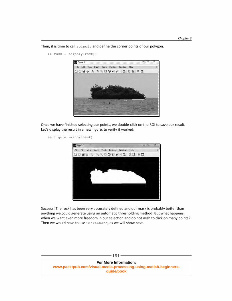
Then, it is ti me to call roipoly and defi ne the corner points of our polygon:

>> mask = roipoly(rock);

Once we have fi nished selecti ng our points, we double-click on the ROI to save our result. Let's display the result in a new fi gure, to verify it worked:

>> figure,imshow(mask)

Success! The rock has been very accurately defi ned and our mask is probably bett er than anything we could generate using an automati c thresholding method. But what happens when we want even more freedom in our selecti on and do not wish to click on many points? Then we would have to use imfreehand, as we will show next.


guide/book



[ 80 ]

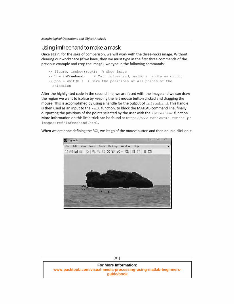
Using imfreehand to make a maskOnce again, for the sake of comparison, we will work with the three-rocks image. Without clearing our workspace (if we have, then we must type in the fi rst three commands of the previous example and crop the image), we type in the following commands:

>> figure, imshow(rock); % Show image>> h = imfreehand; % Call imfreehand, using a handle as output>> pos = wait(h); % Save the positions of all points of the selection

Aft er the highlighted code in the second line, we are faced with the image and we can draw the region we want to isolate by keeping the left mouse butt on clicked and dragging the mouse. This is accomplished by using a handle for the output of imfreehand. This handle is then used as an input to the wait functi on, to block the MATLAB command line, fi nally outputti ng the positi ons of the points selected by the user with the imfreehand functi on. More informati on on this litt le trick can be found at http://www.mathworks.com/help/images/ref/imfreehand.html.

When we are done defi ning the ROI, we let go of the mouse butt on and then double-click on it.


guide/book


Chapter 3

[ 81 ]

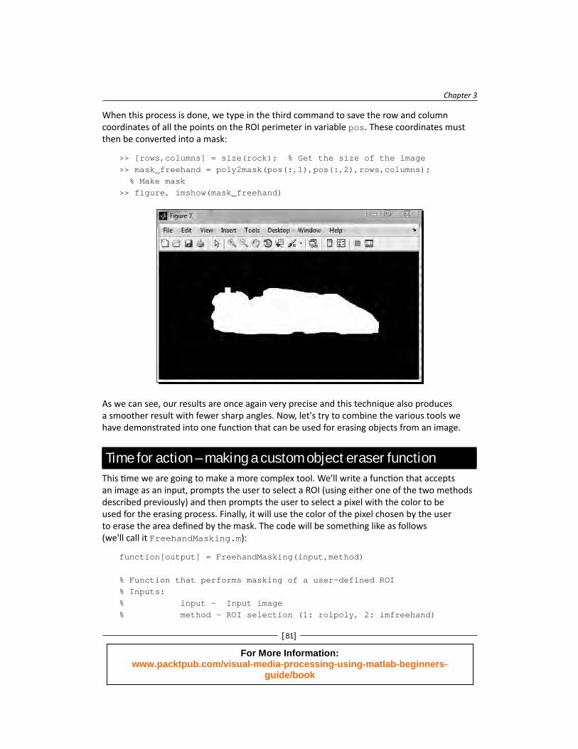
When this process is done, we type in the third command to save the row and column coordinates of all the points on the ROI perimeter in variable pos. These coordinates must then be converted into a mask:

>> [rows,columns] = size(rock); % Get the size of the image>> mask_freehand = poly2mask(pos(:,1),pos(:,2),rows,columns); % Make mask>> figure, imshow(mask_freehand)

As we can see, our results are once again very precise and this technique also produces a smoother result with fewer sharp angles. Now, let's try to combine the various tools we have demonstrated into one functi on that can be used for erasing objects from an image.

Time for action – making a custom object eraser functionThis ti me we are going to make a more complex tool. We'll write a functi on that accepts an image as an input, prompts the user to select a ROI (using either one of the two methods described previously) and then prompts the user to select a pixel with the color to be used for the erasing process. Finally, it will use the color of the pixel chosen by the user to erase the area defi ned by the mask. The code will be something like as follows (we'll call it FreehandMasking.m):

function[output] = FreehandMasking(input,method)

% Function that performs masking of a user-defined ROI% Inputs:% input - Input image% method – ROI selection (1: roipoly, 2: imfreehand)


guide/book



[ 82 ]

% Output:% output - Output image (masked)

switch methodcase 1mask = roipoly(input);););% Select ROI using roipolycase 2figure, imshow(input)h = imfreehand; % Select ROI using imfreehandpos = wait(h);[rows,columns] = size(input); mask = poly2mask(pos(:,1),pos(:,2),rows,columns);endpix = impixel(input); % Select pixel with eraser coloroutput = input; % Set output equal to inputoutput(mask) = pix(1); % Perform masking to erase selected object

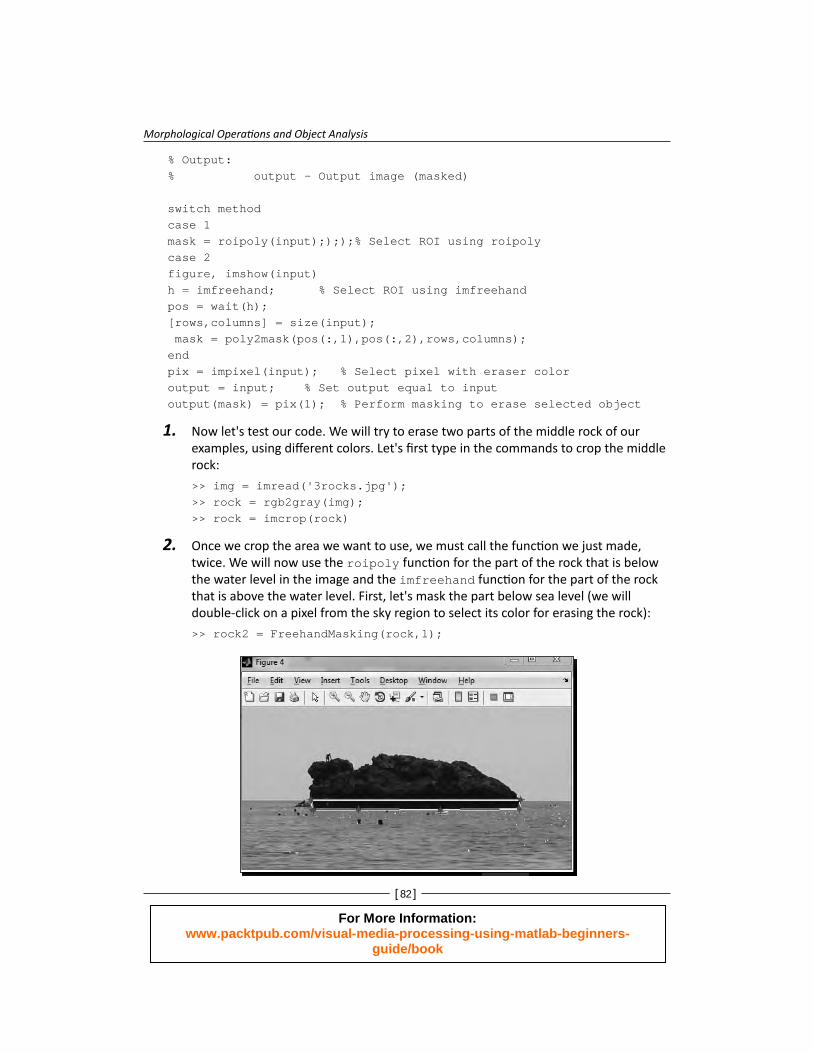
1. Now let's test our code. We will try to erase two parts of the middle rock of our examples, using diff erent colors. Let's fi rst type in the commands to crop the middle rock:

>> img = imread('3rocks.jpg');>> rock = rgb2gray(img);>> rock = imcrop(rock)

2. Once we crop the area we want to use, we must call the functi on we just made, twice. We will now use the roipoly functi on for the part of the rock that is below the water level in the image and the imfreehand functi on for the part of the rock that is above the water level. First, let's mask the part below sea level (we will double-click on a pixel from the sky region to select its color for erasing the rock):

>> rock2 = FreehandMasking(rock,1);


guide/book


Chapter 3

[ 83 ]

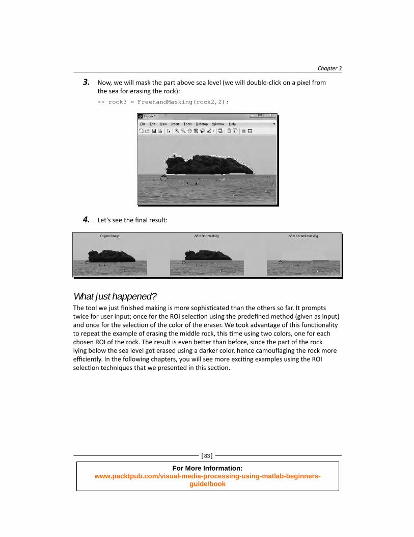
3. Now, we will mask the part above sea level (we will double-click on a pixel from the sea for erasing the rock):

>> rock3 = FreehandMasking(rock2,2);

4. Let's see the fi nal result:

What just happened?The tool we just fi nished making is more sophisti cated than the others so far. It prompts twice for user input; once for the ROI selecti on using the predefi ned method (given as input) and once for the selecti on of the color of the eraser. We took advantage of this functi onality to repeat the example of erasing the middle rock, this ti me using two colors, one for each chosen ROI of the rock. The result is even bett er than before, since the part of the rock lying below the sea level got erased using a darker color, hence camoufl aging the rock more effi ciently. In the following chapters, you will see more exciti ng examples using the ROI selecti on techniques that we presented in this secti on.


guide/book



[ 84 ]

Analyzing objects in an imageAnother main functi on of image processing is the analysis of image content (binary or other). When analyzing an image, usually we search for the presence of edges, corners, or circles inside it. Having this informati on at hand, we are in the positi on to detect shapes and locate specifi c objects in our images, or enhance selected parts of the image. This has a lot to do with the subject of ROI selecti on that we have discussed so far in this chapter. Let's start our image analysis techniques' overview with the most popular method, which is edge detecti on.

Detecting edges in an imageEdge detecti on is a process that typically transforms a grayscale image to a binary one, denoti ng all the pixels belonging to lines of diff erent orientati ons with instances of 1. The edge detecti on process is widely used and has been tackled using a variety of techniques. MATLAB has an inherent functi on called edge, which has incorporated most of the popular methods in an easily usable form.

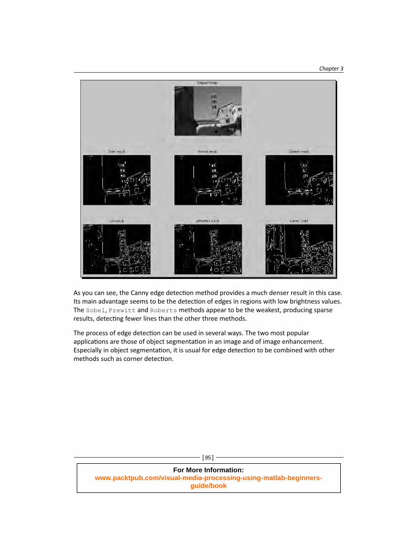
To demonstrate the process, we will use an image with many lines, so that the usefulness of each algorithm is demonstrated. The one chosen is holiday_image2.bmp. To get a bett er idea of all the diff erent methods supported by edge, you can type help edge in the command line. These methods are Sobel, Prewitt, Roberts, Laplacian of Gaussian (LoG), zero-cross and Canny. Let's use them all for our images and display the results. In order for the edge detecti on to perform faster, we will fi rst resize our image by a scale of 0.5:

>> img = imread('holiday_image2.bmp');>> img = imresize(img,0.5);>> BW1 = edge(img,'sobel');>> BW2 = edge(img,'prewitt');>> BW3 = edge(img,'roberts');>> BW4 = edge(img,'log');>> BW5 = edge(img,'zerocross');>> BW6 = edge(img,'canny');>> subplot(3,3,2),imshow(img),title('Original Image')>> subplot(3,3,4),imshow(BW1),title('Sobel result')>> subplot(3,3,5),imshow(BW2),title('Prewitt result')>> subplot(3,3,6),imshow(BW3),title('Roberts result')>> subplot(3,3,7),imshow(BW4),title('LoG result')>> subplot(3,3,8),imshow(BW5),title('Zerocross result')>> subplot(3,3,9),imshow(BW6),title('Canny result')


guide/book


Chapter 3

[ 85 ]

As you can see, the Canny edge detecti on method provides a much denser result in this case. Its main advantage seems to be the detecti on of edges in regions with low brightness values. The Sobel, Prewitt and Roberts methods appear to be the weakest, producing sparse results, detecti ng fewer lines than the other three methods.

The process of edge detecti on can be used in several ways. The two most popular applicati ons are those of object segmentati on in an image and of image enhancement. Especially in object segmentati on, it is usual for edge detecti on to be combined with other methods such as corner detecti on.


guide/book



[ 86 ]

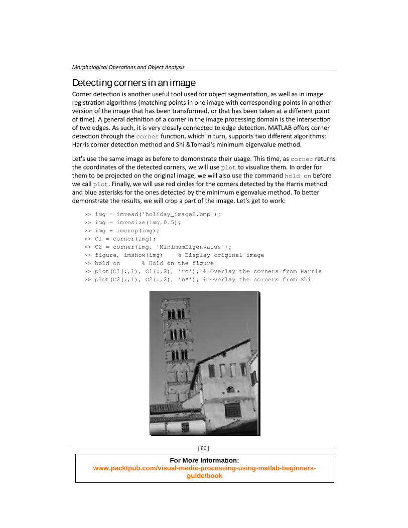
Detecting corners in an imageCorner detecti on is another useful tool used for object segmentati on, as well as in image registrati on algorithms (matching points in one image with corresponding points in another version of the image that has been transformed, or that has been taken at a diff erent point of ti me). A general defi niti on of a corner in the image processing domain is the intersecti on of two edges. As such, it is very closely connected to edge detecti on. MATLAB off ers corner detecti on through the corner functi on, which in turn, supports two diff erent algorithms; Harris corner detecti on method and Shi &Tomasi's minimum eigenvalue method.

Let's use the same image as before to demonstrate their usage. This ti me, as corner returns the coordinates of the detected corners, we will use plot to visualize them. In order for them to be projected on the original image, we will also use the command hold on before we call plot. Finally, we will use red circles for the corners detected by the Harris method and blue asterisks for the ones detected by the minimum eigenvalue method. To bett er demonstrate the results, we will crop a part of the image. Let's get to work:

>> img = imread('holiday_image2.bmp');>> img = imresize(img,0.5);>> img = imcrop(img);>> C1 = corner(img);>> C2 = corner(img, 'MinimumEigenvalue');>> figure, imshow(img) % Display original image>> hold on % Hold on the figure>> plot(C1(:,1), C1(:,2), 'ro'); % Overlay the corners from Harris>> plot(C2(:,1), C2(:,2), 'b*'); % Overlay the corners from Shi


guide/book


Chapter 3

[ 87 ]

The results show that the Shi-Tomasi method produces more results using the default setti ngs and that most of the results coincide. However, they are not completely identi cal, so we must be careful when choosing which technique to use.

Detecting circles in an imageThe last of the popular image processing methods we will visit, which is widely used in everyday tasks, is circle detecti on. Circles are a very descripti ve feature of many objects that oft en need to be detected in an image. To name a few, circle detecti on can be used to localize eyes, stars, balls, coins, ti res, lights, and so on. MATLAB's inherent functi on for circle detecti on is functi on imfindcircles. It can be used with several possible inputs, with the only ones necessary being the input image and the radius (or range of radii) in pixels of the circle we want to detect. Its output may be only the centers of the detected circles, or it can also contain the radii of the respecti ve circles and the power of each circle.

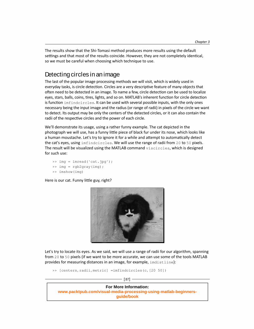
We'll demonstrate its usage, using a rather funny example. The cat depicted in the photograph we will use, has a funny litt le piece of black fur under its nose, which looks like a human moustache. Let's try to ignore it for a while and att empt to automati cally detect the cat's eyes, using imfindcircles. We will use the range of radii from 20 to 50 pixels. The result will be visualized using the MATLAB command viscircles, which is designed for such use:

>> img = imread('cat.jpg');>> img = rgb2gray(img);>> imshow(img)

Here is our cat. Funny litt le guy, right?

Let's try to locate its eyes. As we said, we will use a range of radii for our algorithm, spanning from 20 to 50 pixels (if we want to be more accurate, we can use some of the tools MATLAB provides for measuring distances in an image, for example, imdistline):

>> [centers,radii,metric] =imfindcircles(c,[20 50])


guide/book



[ 88 ]

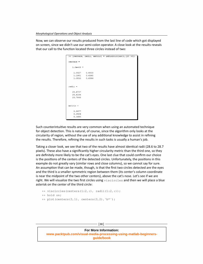
Now, we can observe our results produced from the last line of code which got displayed on screen, since we didn't use our semi-colon operator. A close look at the results reveals that our call to the functi on located three circles instead of two:

Such counterintuiti ve results are very common when using an automated technique for object detecti on. This is natural, of course, since the algorithm only looks at the circularity of region, without the use of any additi onal knowledge to assist in refi ning the results. Therefore, refi ning the results in such tasks is usually a human's job.

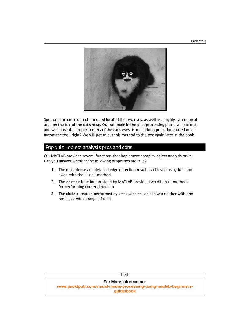
Taking a closer look, we see that two of the results have almost identi cal radii (28.6 to 28.7 pixels). These also have a signifi cantly higher circularity metric than the third one, so they are defi nitely more likely to be the cat's eyes. One last clue that could confi rm our choice is the positi ons of the centers of the detected circles. Unfortunately, the positi ons in this example do not greatly vary (similar rows and close columns), so we cannot say for sure. An assumpti on that can be made, though, is that the fi rst two circles detected are the eyes and the third is a smaller symmetric region between them (its center's column coordinate is near the midpoint of the two other centers), above the cat's nose. Let's see if we are right. We will visualize the two fi rst circles using viscircles and then we will place a blue asterisk on the center of the third circle:

>> viscircles(centers(1:2,:), radii(1:2,:));>> hold on;>> plot(centers(3,1), centers(3,2),'b*');


guide/book


Chapter 3

[ 89 ]

Spot on! The circle detector indeed located the two eyes, as well as a highly symmetrical area on the top of the cat's nose. Our rati onale in the post-processing phase was correct and we chose the proper centers of the cat's eyes. Not bad for a procedure based on an automati c tool, right? We will get to put this method to the test again later in the book.

Pop quiz – object analysis pros and cons

Q1. MATLAB provides several functi ons that implement complex object analysis tasks. Can you answer whether the following properti es are true?

1. The most dense and detailed edge detecti on result is achieved using functi on edge with the Sobel method.

2. The corner functi on provided by MATLAB provides two diff erent methods for performing corner detecti on.

3. The circle detecti on performed by imfindcircles can work either with one radius, or with a range of radii.


guide/book

www.packtpub.com/visual-media-processing-using-matlab-beginnersguide/


[ 90 ]

SummaryIn this chapter, we presented several useful morphology-based techniques for selecti ng regions of interest and masking an image. Aft er visiti ng several examples based on the morphology theory, we also provided an introductory presentati on of some powerful object analysis tools that can be used for several image processing applicati ons such as image enhancement, object detecti on, image registrati on, and so on. The focus of this chapter was on hands-on, practi cal examples demonstrati ng the signifi cance of the methods presented. More specifi cally, in this chapter we covered:

What binary images are and how we can create them using automati c thresholding techniques.

How we can refi ne a region of interest to bett er suit our needs, using dilati on (imdilate) and erosion (imerode) to perform enlargement and shrinking, respecti vely.

What structuring elements are and how they aff ect the quality of dilati on and erosion results.

What masking is and how we can use it to process specifi c regions of interest in an image.

How to manually select a region of interest in order to defi ne bett er masks for our applicati ons, using roipoly and imfreehand.

How to detect edges in a grayscale image using functi on edge.

How to detect corners in an image using functi on corner.

How to detect circles in an image with imfindcircles.

In the next chapter, we will expand the methods we have discussed so far to color image processing. We will produce new functi ons to implement our functi ons to color images and provide specialized soluti ons that take advantage of the extra informati on included in these cases. At the end of the chapter, you will be able to manipulate and process color pictures to produce results that look more appealing and even apply arti sti c eff ects that give your photographs a more professional look.


guide/book


Where to buy this book You can buy Visual Media Processing Using MATLAB Beginner's Guide from the Packt Publishing website: http://www.packtpub.com/visual-media-processing-using-matlab-beginners-guide/book. Free shipping to the US, UK, Europe and selected Asian countries. For more information, please read our shipping policy.

Alternatively, you can buy the book from Amazon, BN.com, Computer Manuals and most internet book retailers.

www.PacktPub.com


guide/book

http://www.packtpub.com/Shippingpolicy


visual media processing using matlab beginner's guide

Documents