vision based data fusion for autonomous vehicles target tracking using interacting multiple dynamic...

www.elsevier.com/locate/cviu

Computer Vision and Image Understanding 109 (2008) 1–21

Vision based data fusion for autonomous vehicles target trackingusing interacting multiple dynamic models

Zhen Jia a,*, Arjuna Balasuriya b, Subhash Challa c

a United Technologies Research Center, Shanghai, 201206, P.R. Chinab Department of Mechanical Engineering, MIT, Cambridge, MA 02139, USA

c Information and Communication Group, Faculty of Engineering, The University of Technology, Sydney, Australia

Received 29 March 2004; accepted 1 December 2006Available online 23 December 2006

Abstract

In this paper, a novel algorithm is proposed for the vision-based object tracking by autonomous vehicles. To estimate the velocity ofthe tracked object, the algorithm fuses the information captured by the vehicle’s on-board sensors such as the cameras and inertial motionsensors. Optical flow vectors, color features, stereo pair disparities are used as optical features while the vehicle’s inertial measurementsare used to determine the cameras’ motion. The algorithm determines the velocity and position of the target in the world coordinate whichare then tracked by the vehicle. In order to formulate this tracking algorithm, it is necessary to use a proper model which describes thedynamic information of the tracked object. However due to the complex nature of the moving object, it is necessary to have robust andadaptive dynamic models. Here, several simple and basic linear dynamic models are selected and combined to approximate the unpre-dictable, complex or highly nonlinear dynamic properties of the moving target. With these basic linear dynamic models, a detaileddescription of the three-dimensional (3D) target tracking scheme using the Interacting Multiple Models (IMM) along with an ExtendedKalman Filter is presented. The final state of the target is estimated as a weighted combination of the outputs from each different dynamicmodel. Performance of the proposed fusion based IMM tracking algorithm is demonstrated through extensive experimental results.� 2006 Elsevier Inc. All rights reserved.

Keywords: Optical flow; Extended Kalman Filtering; Image segmentation and clustering; Stereo vision; Target tracking; Autonomous vehicles; Lineardynamics model; Kinematic model; Interacting multiple models (IMM); Pinhole camera projection model; Template matching and updating; Sensor datafusion

1. Introduction

Computer vision for Autonomous Guided Vehicle(AGV) navigation has been an active research area for a verylong time [8]. This paper proposes a vision based trackingalgorithm whose potential applications are: autonomousvehicles target following and obstacle avoidance [8]. Forsuch applications the tracking system is expected to providethe complete 3D information of the target in the world coor-dinate with a moving environment, i.e., the target’s size, loca-tion, velocity, and depth (distance) [10].

In most of the proposed target tracking algorithms,autonomous vehicles burden the target with special equip-

1077-3142/$ - see front matter � 2006 Elsevier Inc. All rights reserved.

doi:10.1016/j.cviu.2006.12.001

* Corresponding author. Fax: +86 21 58998020.E-mail address: [email protected] (Z. Jia).

ments, for example the intelligent space (ISpace) from [23].Generally in some unknown environments or outdoor situ-ations, such special sensors may not be available for exper-imental testing. Thus in order to achieve a more robusttarget tracking, the vehicle’s on-board sensors should esti-mate the motion parameters of the tracking object accu-rately. These sensors detect the relative dynamics betweenthe autonomous vehicle and target.

Using on-board sensors for target tracking imposes fourmajor challenges [8].

• First, as the vision sensors (CCD stereo cameras pair) aremoving with the vehicle, the background changes contin-uously. With a changing background, it is hard to identifythe object’s dynamics based only on the vision sensors.

mailto:[email protected]

2 Z. Jia et al. / Computer Vision and Image Understanding 109 (2008) 1–21

• Second, for autonomous vehicles in the outdoor envi-ronment, the optical properties of the target may beunpredictable or inconsistent (such as the changes inthe environmental lighting condition) making the fea-ture extraction extremely difficult.

• Third, previous visual target tracking systems estimatethe relative position and velocity of the object to thevehicle. In order to achieve more general applicationswith the target’s dynamic information and obtain moreaccurate estimation results, the target’s 3D velocityand position need to be estimated in the worldcoordinate.

• Fourth, natural moving targets often have unpredict-able, complex or highly nonlinear motion dynamics.Commonly used linear models will not produce thesedynamic properties.

The motivation of this paper is to develop a data fusionbased target tracking system to solve the above problems.The novelty of this paper is the combination of differentdata fusion techniques to achieve a reliable tracking sys-tem. Normally data fusion can be achieved either by usingmultiple (redundant) sensors or by combining several mea-surements of a single sensor [30]. In this paper, three differ-ent data fusion steps are developed and integrated togetherto formulate the novel tracking scheme.

• First, different visual features from CCD camerasare fused to accurately extract the region of interest(ROI) from the image sequence with a changing back-ground.Most of the vision-based tracking schemes depend onoptical properties of the object of interests [31]. This cre-ates practical difficulties when these features change inthe scene, which is the case with objects in complex envi-ronments such as underwater. Thus the aim of thispaper is to use motion fields in the scene rather thanusing any special property of the object for target iden-tification and tracking, which is quite challenging.Optical flow vectors reflect the motion of target pixelsin the image sequence, and it requires a minimal priorknowledge of the observed environment. From the pre-vious research work [7,18,26,32,33], by fusing opticalflow vectors with the target’s other visual features, areliable object tracking system could be designed totrack the object’s 3D state. Also optical flow vectorscan be employed as the velocity measurements fortracking the boundaries of the nonrigid objects suchas the method of Kalman Snakes [28]. In this paperoptical flow vectors are used as the main source forthe target’s 3D features identification [18]. First, opticalflow vectors are fused with the image various visualfeatures to segment the motion fields, which is usedto identify the region of interest (ROI) from back-ground motion fields. Next, optical flow vectors arefused with the motion sensors data to estimate thetarget’s 3D velocity and position.

• Secondly, the vision sensor data are fused with thevehicle’s inertial motion sensors data for estimatingthe target’s position and velocity in the 3D world coor-dinate frame.In this paper the kinematic model of the autonomousvehicle is used to estimate the velocity of the cameras’motion based on the vehicle’s inertial sensors. The kine-matic model is able to provide information such as selfrotation/translation about/along the optical axis. Nextoptical flow vectors are fused with the moving cameras’motion parameters based on the motion compensationapproach [5]. In such a way, the target’s 3D velocityand position are estimated in the world coordinate forthe MCMO target tracking.

• Thirdly, several simple and basic linear dynamic mod-els are fused with the multiple models algorithm toapproximate the target’s complex motion propertiesfor an accurate target tracking.In visual target tracking, the dynamic information aidsthe tracking process in the presence of occlusions andmeasurement noises [16]. However, the tracking is com-plicated by the fact that natural moving targets do notexhibit one type of motion but rather have complex,unknown, highly nonlinear or time-varying dynamics.The single model approaches do not make full use ofthe information available and often rely on somewhatad hoc methods of incorporating uncertainty aboutthe mode estimates (like adjusting the filter noisecovariance in proportion to the variances in the modelestimate [18]), so the traditional single linear dynamicmodels are not quite applicable. Tracking of such tar-gets falls into the area of adaptive state estimation(multiple models methods) [9,19].The distinguishing feature of multiple models approach-es is a stochastic (typically Markov) process switchingbetween the models and the simultaneous filtering ofthe observations through all of the possible systems.The final state estimate is obtained as a weighted combi-nation of the outputs of estimates from each differentmodel, which is in contrast to single model algorithmsthat tend to use one model at any given time.Recently Forsyth et al. [13] reviewed the linear dynamicmodels for target tracking. These models are quite simpleand easy to implement and cover most of the target’s lin-ear dynamic properties. In the proposed tracking system,these simple linear dynamic models are combined togeth-er with the multiple models algorithm to represent thetarget’s complex motion properties.Research works have been carried out in target trackingusing Multiple Models (MM) filtering. Bar-Shalom andLi [1] reviewed the models in which both the statedynamics and output matrices switch, and the switchingfollows the Markovian dynamics (IMM). They have alsopresented several different methods for approximatelysolving the state-estimation problems in switching mod-els. Some other multiple models tracking systems use theBayesian network based multi-model fusion methods

Z. Jia et al. / Computer Vision and Image Understanding 109 (2008) 1–21 3

[11], and [21]. More recently, switching linear dynamicsystem (SLDS) models have been studied in [3]. SLDSmodels and their equivalents have also been studied instatistics, time-series modelling, and target tracking sincethe early 1970’s in [27]. It is concluded by Bar-Shalom [1]that the IMM algorithm performs significantly betterthan other multiple models methods. It computes thestate estimates under each possible current model usingseveral filters, with each filter using a different combina-tion of the previous model-conditioned estimates (mixedinitial condition). The mixed initial condition of IMMcan reduce the estimation errors by adjusting the initialcondition for each estimate. IMM is also faster in com-putation than other multiple models algorithms, forexample IMM requires only r filters to operate in parallelwhile the generalized pseudo-Bayesian (GPB) multiplemodels algorithm requires r or r2 to operate in parallel.Furthermore, the IMM has been shown to be able tokeep the estimation errors not worse than the raw mea-surement errors and provide significant improvements(noise reduction).In this paper the IMM approach is developed to fuse sev-eral simple and basis linear dynamic models for the tar-get dynamic information tracking. The interactingmultiple linear dynamic models algorithm provides anapproximation of the types of the target’s employedmotion, and then the target’s dynamic state estimatesare obtained with the combination of the weighted differ-ent models’ Extended Kalman Filter estimates, whichcan improve the tracking performance. The InteractingMultiple Models (IMM) algorithm here also allows thesystem to minimize tracking errors by adjusting the gainof the Extended Kalman Filter.

Fig. 1. The proposed

The rest of this paper is organized as follows: In Section2, the proposed tracking system is described. Section 3talks about the data fusion based K-means image segmen-tation and clustering and template matching algorithms. InSection 4, optical flow vectors are fused with the target’sdepth disparities information and then combined with thekinematic model of the camera system to estimate the tar-get’s 3D position and velocity in the world coordinate.With the target dynamic features, several simple lineardynamic models with the IMM algorithm are used to con-duct the target Extended Kalman Filter tracking in Section5. Section 6 presents the extensive experimental resultsobtained by nature image sequences. Section 7 concludesthe research work in this paper and makes suggestionsfor future work.

2. Proposed tracking system

The proposed tracking scheme has the ability to trackthe target’s 3D dynamics in an unknown environment inthe Moving Camera and Moving Object (MCMO) state[25]. From the literature reviews [15], the prerequisites foreffectively tracking the moving target using CCD camerasgenerally include detection of features (feature segmenta-tion and classification) and target tracking. In such away, the novel tracking methodology is designed basedon the strategies shown in Fig. 1.

In the first step, the stereo images are captured fromCCD cameras. In order to accurately identify the targetfrom the image sequences with a changing background,the image motion properties (optical flow vectors) areextracted from the image sequence. Since the system isdesigned to track the target’s 3D dynamics, the target’s

tracking system.


3D visual depth is estimated from stereo images. In the sec-ond step, because different objects have different visual fea-tures, for example the motion properties and there are alsobackground features together with the target’s features,these visual features are classified and localized by theimage processing algorithms such as image clustering andtemplate matching to find the useful ones. In the third step,optical flow vectors are fused with the target’s depth dis-parity information and then combined with the kinematicmodel of the camera system to estimate the target’s 3Dposition and velocity in the world coordinate. These infor-mation is used later for the target dynamics tracking. In thefinal step, the target 3D dynamics is estimated with Extend-ed Kalman Filter. Through the Extended Kalman Filtermeasurement equation, sensor data fusion is achieved forthe proposed tracking scheme. In the final step, several sim-ple and basic linear dynamic models with the IMMapproach are used to make the approximation of the targetcomplex motion properties.

3. Fusion based image segmentation and clustering and

template matching

In this paper, the image motion fields are clustered tofind the major motion regions. As long as the motionregion’s optical flow vectors are not zero, they can be suc-cessfully clustered out from the image sequence even if theyare less accurately estimated. Therefore, the most common-ly used Horn and Schunck’s differential (gradient-based)technique is tested for the calculation of optical flow dueto its fast computational speed, easiness to implement,100% density and accuracy [2,14]. At the same time, thedisparity (denoted as d) is estimated from the stereo imag-es. This paper chooses the normally used and simple Sumof the Absolute RGB Differences (SAD) algorithm to esti-mate the disparity d. The Sum of Absolute RGB Differenc-es (SAD) performs better than the normally used Sum ofSquared Differences in the presence of outliers [24]. Usingcolor information instead of gray values improves the sig-nal to noise ratio by 0.2–0.5.

Next, in the case of target tracking by autonomous vehi-cles, one big challenge is to separate the optical flow vectorsfield of the target from the background motion field.Assuming that the moving target is a rigid object with uni-form motion properties within its body (the assumption isquite reasonable for the normal target tracked by autono-mous vehicles.), the target region can be identified from thebackground with the motion vectors clustering and seg-mentation [18].

Recently some research works have been done on themotion based image segmentation [4,6,12]. These kinds ofwork do the optical flow estimation and image segmenta-tion simultaneously. As stated earlier, the optical flow esti-mation is based on the classic Horn and Schunck’s method.The image segmentation needs a separate and simplemethod. Therefore the well-known K-means algorithm isapplied to segment the optical flow vectors field by dividing

the image scene into different clusters. The feature set usedin the K-means algorithm is given in Eq. (1).

~x ¼ ½vx; vy ; x; y;R;G;B� ð1Þwhere x, y are the pixel’s locations in the 2D images, vx

and vy are the optical flow vectors and R, G, B are theintensities of the color components at that pixel point.The RGB color space instead of the HSV color space isused here because the RGB color values can be readdirectly from the image and it is much easier for the algo-rithm implementation.

The distance between two feature vectors is measuredusing a Mahalanobis distance, defined by

dð~x1;~x2Þ ¼X

K-means

ð~x1 �~x2ÞTS�1ð~x1 �~x2Þ ð2Þ

whereP

K-means ¼ diagð1; 1; 1; 1; 2; 2; 2Þ. S�1 is the inverseof the variance–covariance matrix of ~x. The purpose ofthe matrix

Pis to weight the color intensities since they

are of different scales (and units) from the other 4 compo-nents in the feature vector. The color features can be gen-erally weighted more than the others since normally thecolor information is more apparent and is the dominatingvisual feature [18]. After some trial-and-error,P

K-means ¼ diagð1; 1; 1; 1; 2; 2; 2Þ inP

for the RGB compo-nents is found to give good results.

Here, the target’s optical flow vectors are fused with thecolor and spatial information to make the image segmenta-tion and clustering more robust. The object is assumed tobe a rigid one with uniform motion. Integration of colorwith motion fields solves some of the image segmentationproblems. For example, if the object is a textured one withdifferent visual color properties, the K-means algorithmstill can make an accurate clustering based on the object’suniform motion properties from the image sequences.

In this paper, 5 and 3 clusters are generally selected forthe natural video images K-means clustering. This numbercan be determined automatically for video images segmen-tation by incorporating the intra-cluster and inter-clusterdistance validity measures developed by [29]. There is a ten-dency to select smaller cluster numbers for natural images,which is due to the inter-cluster distance being much great-er and greatly affecting the validity measures. The normalsmallest number of clusters that can be selected is 4 [29].In fact the clusters’ number may be changed. With moreimage clusters, the video images segmentation may be moreaccurate while at the same time the computational time willalso increase. Also the number of clusters in the experi-ments can be adapted to the contents of the video frames.For example, a small number of clusters for the objectbased image segmentation of frames with 10 objects istoo ambiguous, even though the object of interest can bewell covered. So when the background is very clutteredand there are more objects like 8–10 in the image, 8–9 clus-ters would be more appropriate. If there are fewer majorobjects like 3–5 or the environment is structured, 3–5 clus-ters would be all right.


After the image segmentation and clustering, the majormotion regions are left in the clustered optical flow vectorsfield. The smaller motion regions considered as noise areremoved. A template is defined and correlated with theclustered optical flow vectors fields to extract the ROI fromthe background motion field. The template is the target’sregion in the 2D clustered optical flow vectors field. Thematching is done with the simple cost function by thesum of squared differences (SSD) between the templateand the whole clustered motion vectors field.

SSD ¼XjjT � I jj2 ð3Þ

where T is the template and I is the clustered optical flowvectors field. The minimization of the SSD (Eq. (3)) is ob-tained by sequentially scanning the whole optical flow vec-tors field and finding the minimum value of Eq. (3). Thecoordinates of the ROI are considered as the 2D positionof the target in the image, which are used in the next sec-tion for estimating the target’s 3D dynamics in the worldcoordinate.

The template consists of only optical flow vectors, thusthe extraction of the ROI’s 2D position is carried out onlywith the target’s dynamic features, which can make thetracking system robust to localize targets independent oftheir other visual features such as shape or color. Forexample, if a target is moving in the images and its colorchanges, template matching using color information maygo wrong. In such a situation, the target’s motion is stillthe same, so the template matching by optical flow vectorscan give better results. Also using the 2D motion vectorsinstead of the image’s 3D RGB color information reducesthe whole system’s computational cost.

At present, the initial template can be automaticallyidentified from the clustered optical flow motion field ifthere is only one target moving or only one new objectentering the image scene for tracking. If there are severalobjects moving together in the image, the initial templatemust be selected manually from the first clustered opticalflow vectors field because the tracking algorithm does nothave the intelligence to tell which object is of interest. InSection 6, the tracker’s automatic initialization, terminationor multiple people tracking are discussed with experimentalresults. After the matching template is initialized, thematching value (Eq. (3)) should be very small when the tar-get is moving in the image scene. If the matching value ismuch larger than a preset threshold, it means that the targethas exited and the tracker should be automatically termi-nated. During the tracking process, the template is updatedframe by frame with the target’s previous estimated 3Ddynamic information. This updating process is known asthe ‘‘naive update’’ template updating algorithm [22].

4. Sensor data fusion for target’s 3D dynamic information

estimation

Once the target is identified in the image scene, it is thennecessary to estimate its velocity and position to track it by

autonomous vehicles. This section presents the proposedestimation procedures.

In this paper, the target’s 3D position and velocity inthe world coordinate are estimated for the visual targettracking system. In the previous autonomous vehiclestarget tracking systems, the target’s relative dynamicinformation from CCD cameras is used directly for thenavigation purpose. There are several drawbacks usingthe relative information in autonomous vehicles targettracking. First, these data are only relative from thevision sensors to the target, which are not available forother applications in the same environment. Secondly,in such a situation the vehicle’s self rotational and trans-lational motion in the world coordinate are generally notconsidered, which makes the target dynamics estimationless accurate. So in the proposed visual target trackingscheme, in order to achieve more general applicationsand get more accurate estimation results than the meth-ods like [7,8,33], the target’s 3D velocity and position areestimated in the world coordinate. For this purpose, thecameras’ motion parameters should be known and there-fore the moving vehicle’s kinematic model should beintegrated in the tracking system. With the kinematicmodel of the vehicle, tracking problems involving thecameras’ 3D motion can also be solved.

Let’s first consider the cameras mounted on an autono-mous vehicle moving in the 3D world coordinate as shownin Fig. 2a. Estimation of the target’s velocity can beachieved using the algorithm explained in Fig. 2b. Here,the motion of the target in the image stream is obtainedas optical flow vectors ~V O:F :

T . Then ~V O:F :T is transformed into

the image coordinate frame as ~V IMT . Next ~V IM

T is trans-formed into the camera frame to get the target velocity rel-ative to the cameras ~V C

T .Because the cameras are moving in the world coordi-

nate, its axis has the rotational motion RWC and transla-

tional motion T WC relative to the world coordinate. The

velocity of the moving cameras in the world coordinate~V W

C (consists of RWC and T W

C ) can be estimated based onthe kinematic model of the autonomous vehicle. Thenthe target’s velocity in the world coordinate ~V W

T can beestimated as:

~V WT ¼ RW

C � ~V CT þ T W

C ð4Þ

This equation shows how the visual features can be fusedwith the cameras’ motion parameters for estimating thetarget’s velocity.

The following section first explains how ~V CT is estimated.

Here, the 2D visual cues are fused with the disparity infor-mation using a pinhole camera projection model (Fig. 3and Eq. (5)) to obtain the target’s 3D velocity relative tothe cameras.

x

y

� �¼ f

Z

X

Y

� �ð5Þ

The time derivation of Eq. (5) gives the velocity.

Fig. 2. Experiment setup with the target’s 3D world coordinate velocity estimation procedures.

Fig. 3. The pinhole camera projection model.


X ¼ Zf

x) _X ¼ _x � Z þ _Z � xf

ð6Þ

where _X is the target’s velocity relative to the camera frameknown as ~V C

T and _x is the target’s image pixel velocity ~V IMT ,

which can be estimated from the optical flow vectors ~V O:F :T

(Eq. (7)).

~V IMT ¼ S � ~V O:F :

T ð7Þ


where S is the effective size of the pixels in the image, whichtransforms the image pixel velocity (optical flow vectors)into the real image coordinate displacement. In Eq. (6), Z

is the target depth information, which can be estimatedfrom the disparity d. The deviation of the depth _Z is ob-tained as _Z ¼ �b1f Dd

d2 , Dd is the difference of the disparityd between two time stamps. From Eqs. (5) and (7), ~V C

T

can be obtained as in Eq. (8)

~V CT ¼

V CT x

V CT y

V CT z

0B@

1CA ¼

1f ð _Z � xþ V IM

T x � ZÞ1f ð _Z � y þ V IM

T y � ZÞ_Z

0BB@

1CCA

¼

1f ð�b1f Dd

d2 � xþ Sx � V O:F :T x � b1

fdÞ

1f ð�b1f Dd

d2 � y þ Sy � V O:F :T y � b1

fdÞ

�b1f Ddd2

0BB@

1CCA ð8Þ

where (x,y) is the target 2D image coordinate, which can beestimated from the previous ROI identification. The stereocameras’ optical axes are parallel and separated by a dis-tance b1.

In order to get the cameras’ rotation and translationmatrixes RW

C and T WC , the cameras’ movement in the world

coordinate should be known. In this paper a simple two-wheel kinematic model for autonomous vehicles is usedfor the experimental testing (Fig. 4). Two tachometers mea-sure the wheels’ velocities v1 and v2. Here u1, u2 are thetachometers’ output voltages, and kT is the linear parame-ter between the tachometers’ output voltages and thewheels velocities, which gives the simple relationshipv1 = kT Æ u1 and v2 = kT Æ u2. In order to simplify the track-ing system, it is just assumed that the wheels’ slippage canbe ignored. The vehicle’s velocity along X and Z directionsin Fig. 4 can then be estimated as Eq. (9).

Fig. 4. The kinematics mode

vX

vZ

_h

0B@

1CA ¼

ðv1þv2Þ cosðhÞ2

ðv1þv2Þ sinðhÞ2

v2�v1

2b

0B@

1CA ¼

ðkT �u1þkT �u2Þ cosðhÞ2

ðkT �u1þkT �u2Þ sinðhÞ2

kT �u2�kT �u1

2b

0BB@

1CCA ð9Þ

where b is the distance between the two wheels and h is theangle between the X axis and the vehicle’s velocity in Fig. 4.

In real world applications, there may be many changes inthe vehicle’s attitude. In order to simplify the algorithm andmake the estimation more accurate, the vehicle’s motion isassumed to be on a flat ground. Therefore, the velocities inthe X and Z directions (Fig. 2a) are considered as the mosteffective movements of the vehicle. The vehicle’s velocity inthe Y-coordinate is too small compared with those of theother two directions and it can be ignored. The camera coor-dinate has only the Y axis rotation relative to the world coor-dinate and the rotational velocities in the other twodirections can be neglected. Based on this assumption, thewhole system becomes much less complex and the followingexperimental results are still good. The whole computation issimplified in a reasonable way. Let h denote the anglebetween the camera velocity and X direction, then the cam-era axis rotation matrix RW

C can be estimated as:

RWC ¼

cosðhÞ 0 � sinðhÞ0 1 0

sinðhÞ 0 cosðhÞ

0B@

1CA; hk ¼ hk�1 þ Dt � _h ð10Þ

Here Dt is the time interval from the time k � 1 to time k toestimate h from _h in Eq. (9). In the following equations, thetime k for h is omitted because all the estimations are doneat the same time stamp k.

At the same time the vehicle’s translational vector in theworld coordinate can be estimated as T W

C . The vehicle onlyhas velocities in the X and Z directions. Based on theautonomous vehicle’s kinematic model, T W

C can be writtenas Eq. (11):

l of autonomous vehicle.


T WC ¼

T WC x

T WC y

T WC z

0B@

1CA ¼

ðkT �u1þkT �u2Þ cosðhÞ2

0ðkT �u1þkT �u2Þ sinðhÞ

2

0B@

1CA ð11Þ

Finally from Eq. (4), (8), (10) and (11), the target’s 3Dvelocity ~V W

T in the world coordinate can be estimated as

V WT x

V WT y

V WT z

0B@

1CA¼

1f ð�b1f Dd

d2 �xþSx �V O:F :T x �b1

fdÞ �cosðhÞ�b1f Dd

d2 � sinðhÞþðkT �u1þkT �u2ÞcosðhÞ2

1f ð�b1f Dd

d2 �yþSy �V O:F :T y �b1f 1

dÞ1f ð�b1f Dd

d2 �xþSx �V O:F :T x �b1

fdÞ �sinðhÞþb1f Dd

d2 �cosðhÞþðkT �u1þkT �u2ÞsinðhÞ2

0BB@

1CCA

ð12Þ

The target’s 3D position in the world coordinate ~P WT can

also be obtained from Eq. (13).

~P WT ¼ RW

C �~P CT þ T W

C ð13Þ

Here RWC is the camera axis’s rotational matrix (Eq. (10)).

~P CT is the target position relative to the cameras in the cam-

era frame. T WC is the translational vector between the cam-

era coordinate and the world coordinate (Eq. (11)). So ~P WT

can be written as:

~P CT ¼

P CT x

P CT y

P CT z

0B@

1CA ¼

Sx�x�Zf

Sy �y�Zf

Z

0B@

1CA

~P WT ¼

cosðhÞ � Sx�x�Zf � sinðhÞ � Z þ t � ðkT �u1þkT �u2Þ cosðhÞ

2

Sy �y�Zf

sinðhÞ � Sx�x�Zf þ cosðhÞ � Z þ t � ðkT �u1þkT �u2Þ sinðhÞ

2

0BB@

1CCA ð14Þ

These equations (Eqs. (12) and (14)) show the data fusionof the target’s optical flow vectors ðV O:F :

T x; VO:F :T yÞ, visual

disparity d, image coordinates (x,y) and motion sensorsdata (u1,u2) into one equation to estimate the target’s 3Dvelocity and position in the world coordinate. These twoequations are used later to obtain the Extended KalmanFilter measurement function for estimating the targetdynamics, which is the proposed data fusion scheme totrack the target dynamic states.

5. Multiple models fusion based target tracking system

At this stage, the position and velocity of the target areestimated together using a Kalman Filter. Since the veloc-ity and position measurement models of the target areobtained from the inverse calculations of Eq. (12) andEq. (14), the derived Kalman Filter will always containnonlinear components. Therefore, an Extended KalmanFilter is used to cater for the nonlinearities present. Inthe tracking exercise the tracked body is assumed to be a

rigid one. Let ~X denote the target’s dynamic state,

~X ¼~P~V

� �. Then the state equation for its movement can

be written as Eq. (15).

~X kþ1 ¼ Ur~X k þ vk ð15Þ

where Ur denotes the target dynamic models,~P ¼ ðP x; P y ; P zÞT denotes the 3D position of the trackedpoint, and ~V ¼ ðV x; V y ; V zÞT denotes its velocity. vk is theGaussian white noise. vk has a 6 · 6 covariance matrixand over the increment from the time k to time k � 1, thisprocess noise enters into both the position and velocitystates.

The coordinate of the tracked point in the 2D image p

can be obtained from the 3D world coordinate by Eq. (16)

P x

P y

� �k

¼ Pð~P kÞ ð16Þ

In the above equation, P denotes the camera’s pinhole pro-jection transformation of a 3D world coordinate point ~Ponto the 2D image coordinate space (Px,Py).

The resulting position and velocity measurement vectorZ for the system can be obtained as given in Eq. (17)

~Zk ¼ Hðk; ~X kÞk þ wk; ~Zk ¼

V O:F :x

V O:F :y

u1

u2

d

x

y

0BBBBBBBBBBB@

1CCCCCCCCCCCA

ð17Þ

~Zk represents the measurements of the target from differentsensors. Hk is the measurement function, which can be ob-tained from Eq. (12) and Eq. (14). It is worth noting thatthis measurement vector ~Zk and measurement functionH(h)k comprise of the optical flow vectors ðV O:F :

T x; VO:F :T yÞ,

disparity d, tachometer sensors data (u1,u2) and image spa-tial information (x,y) into one equation. wk is the measure-ment noise, which has a covariance matrix of 7 · 7. Thisequation (Eq. (17)) provides a scheme to fuse different visu-al cues with the cameras’ motion parameters as the inputsto EKF for tracking the target’s 3D dynamics as the out-puts from EKF.

5.1. Linear dynamic models for extended Kalman filter

There are several simple and basic linear dynamic mod-els available for Extended Kalman Filter to cover the nor-mal dynamic situations of the moving target [13], whichcover all the linear dynamic properties of the movingobject. The dynamic model is achieved by multiplying thestate with some known matrix U as in the motion stateequation (Eq. (15)), and then adding a normal random var-iable of a zero mean and known covariance. The work inthis paper is to apply the IMM algorithm to fuse these sim-ple and basic models to approximate the complex and non-linear properties of the tracking system, which has not been


done by other researchers and also is the novelty of thispaper.

1. Drifting Points Model. If the dynamic model is

Ui ¼ I ð18Þwhere I is the identity matrix. Then the point’s new po-sition is its old position, plus some Gaussian noiseterms. This drifting points dynamic model can be com-monly used for the object where no better dynamicmodel is known.

2. Constant Velocity Model. p gives the position and v givesthe velocity of a point moving with the constant velocity.The constant velocity model is given in Eq. (19).

~X ¼p

v

� �; Ui ¼

I ðDtÞI0 I

� �ð19Þ

3. Constant Acceleration Model. a is the acceleration of apoint moving with a constant acceleration. Then theconstant acceleration model is given in Eq. (20).

~X ¼p

v

a

0B@

1CA; Ui ¼

I ðDtÞI 0

0 I ðDtÞI0 0 I

0B@

1CA ð20Þ

4. Periodic Motion Model. It is assumed that a point ismoving on a line with a periodic movement. Then stackthe position and velocity into a vector ~u ¼ ðp; vÞ andwith the time interval Dt, the periodic motion modelcan be obtained with a forward Euler method as shownin Eq. (21).

~ui ¼~ui�1 þ Dtdudt¼~ui�1 þ DtS~ui�1 ¼

1 Dt

�Dt 1

� �~ui�1

ð21Þ

5.2. Interacting multiple models approach

In the Interacting Multiple Models approach (IMM), itis assumed that the system obeys one of a finite number ofmodels. A Bayesian framework is used here starting withthe prior probabilities of each model being correct. Themodel, assumed to be in effect throughout the process, isone of r possible models (the system is in one of r modes)as fUjgr

j¼1.Then the prior probability that Uj is correct (the system

is in mode j) is shown in Eq. (22).

PfUjjZ0g ¼ ljð0Þ ð22Þ

where Z0 is the prior measurement information andPrj¼1ljð0Þ ¼ 1.

1. Calculation of the mixing probabilities (i,j = 1, . . . , r).The probability that the mode Ui was in effect at k � 1given that Uj is in effect at k conditioned on Zk�1 isEq. (23).

lijjðk � 1jk � 1Þ ¼ 1

�cjpijliðk � 1Þ; �cj ¼

Xr

i¼1

pijliðk � 1Þ

ð23Þ

It is assumed that the model jump process is a Markovprocess (Markov chain) with the known model transi-tion probability pij

pij ¼ PfUðkÞ ¼ UjjUðk � 1Þ ¼ Uig ð24Þ

here li is estimated later from Eq. (29).2. Mixing (j = 1, . . . , r). Starting with the previous estimate

X̂ iðk � 1jk � 1Þ one computes the mixed initial conditionfor the filter matched to Uj(k) as

X̂ 0jðk � 1jk � 1Þ ¼Xr

i¼1

X̂ iðk � 1jk � 1Þlijjðk � 1jk � 1Þ

ð25ÞThe covariance corresponding to the above is

P 0jðk � 1jk � 1Þ ¼Xr

i¼1

lijjðk � 1jk � 1ÞfP iðk � 1jk � 1Þ

þ ½X̂ iðk � 1jk � 1Þ � X̂ 0iðk � 1jk � 1Þ�� ½X̂ iðk � 1jk � 1Þ � X̂ 0jðk � 1jk � 1Þ�0g

ð26Þ

3. Model-matched filtering (j = 1, . . . , r). The estimate Eq.(25) and covariance Eq. (26) are used as the inputs tothe filter matched to Uj(k), which uses the measurementz(k) to yield X̂ jðkjkÞ and Pj(kjk). The likelihood functioncorresponding to the r filters

KjðkÞ ¼ p½zðkÞjUjðkÞ; Zk�1� ð27Þis computed using the mixed initial condition Eq. (25)and associated covariance Eq. (26) as:

KjðkÞ¼ p½zðkÞjUjðkÞ; X̂ 0jðk�1jk�1Þ; P 0jðk�1jk�1Þ�ð28Þ

4. Model probability update (j = 1, . . . , r). It is done asfollows:

ljðkÞ ¼ 1c KjðkÞ�cj; c ¼

Prj¼1

KjðkÞ�cj ð29Þ

where �cj is the expression from Eq. (23).5. Estimate and covariance combination. Combination of

the model-conditioned estimates and covariances is doneaccording to the mixture equations

X̂ ðkjkÞ ¼Xr

j¼1

X̂ jðkjkÞljðkÞ ð30Þ

P ðkjkÞ ¼Xr

j¼1

ljðkÞfP jðkjkÞ þ ½X̂ jðkjkÞ � X̂ ðkjkÞ�

� ½X̂ jðkjkÞ � X̂ ðkjkÞ�0g ð31Þ

Note that the combination is only for output purposes-itis not a part of the algorithm recursions.


5.3. Interacting multiple models for extended Kalman filter

estimation

Recall the basic model equations for the linear ExtendedKalman Filter Eq. (32).

X ðkÞ ¼ Uðk � 1Þ � X ðk � 1Þ þ vðk � 1ÞZðkÞ ¼ CðkÞ � X ðkÞ þ wðkÞ

ð32Þ

where U is the state transition matrix, X is the state vector,v is the process noise, Z is the measurement value, C is theJacobian matrix of the measurement matrix which is usedfor the Extended Kalman Filter updating, and w is themeasurement noise. The actual state estimation and pre-diction equations are given as Eq. (33):

X ðkjk�1Þ¼Uðk�1Þ � X ðk�1jk�1ÞX ðkjkÞ¼X ðkjk�1ÞþGðkÞ � residueðkÞresidueðkÞ¼ ZðkÞ�CðkÞ � X ðkjk�1ÞP ðkjk�1Þ¼Uðk�1Þ � P ðk�1jk�1Þ � Uðk�1ÞþQðk�1ÞSðkÞ¼CðkÞP ðkjk�1ÞCðkÞTþRðkÞ ð33Þ

where residue(k) is the measurement residue, a Gaussianrandom variable with the zero mean and covariance S(k),and R(k) is the covariance of the measurement noise w.

The equation for the filter gain, G, and the covariancematrix, P, of the state prediction are then as Eq. (34):

GðkÞ¼ Pðkjk�1Þ � CðkÞT �ðCðkÞ� Pðkjk�1Þ� CðkÞTþRðkÞÞ�1

PðkjkÞ¼ ðI�GðkÞ � CðkÞÞ � Pðkjk�1Þ ð34Þ

where Q(k) is the covariance of the process noise v, C(k) isthe measurement matrix from Eq. (32) and U(k) is the statetransition matrix from Eq. (32).

According to the Interacting Multiple Models (IMM)approach, several simple linear dynamic models U intro-duced in the previous sections are used as the differentstate transition matrixes (Eq. (15)) for Extended KalmanFiltering. In the IMM algorithm, the likelihood of eachmode-conditioned estimates Kj(k) as shown in Eq. (28) isgenerated with the Extended Kalman Filter measurementresidue residurej(k) (Eq. (33)) as Eq. (36).

KjðkÞ ¼ N ½residuejðkÞ; 0; SjðkÞ� ð35Þ

Now with the different model’s Extended Kalman Filterstate estimate Xj together with the covariance estimate Pj

and based on the above recursive IMM algorithm, the pro-posed data fusion based visual target tracking system canbe achieved.

Based on the Interacting Multiple Models (IMM)approach, the above four simple linear dynamic modelsare fused for Extended Kalman Filter. In the IMM algo-rithm, the likelihood of each mode-conditioned estimatesKj(k) is generated with the Extended Kalman Filter mea-surement residue residurej(k) as Eq. (36).

KjðkÞ ¼ N ½residuejðkÞ; 0; SjðkÞ� ð36Þ

where residuej(k) is the measurement residue, a Gaussianrandom variable with the zero mean and covarianceSj(k). With the different model’s Extended Kalman Filterstate estimate Xj together with the covariance estimate Pj

and based on the recursive IMM algorithm [1], the pro-posed data fusion based visual target tracking system canbe achieved.

6. Experiment results

To evaluate the performance and adjust the parametersof the proposed method, the tracking system has been test-ed under both the indoor and outdoor situations. In theexperiment a moving platform is designed with the motionsensors and CCD cameras. Motion sensors (tachometers)measure the platform’s wheels speed, which estimate thecameras’ velocity based on the vehicle’s kinematic model.Two color CCD cameras (the focus length f = 5.4 mm)are connected with the Hitachi IP5005 image processingcard for the image capturing and processing (the image sizeis 256 · 220, and the capturing rate is 15f/s).

The processing of the video images takes a lot of compu-tational time. The images are captured in a 15 Hz rate, butthe optical flow vectors estimation and stereo disparity cal-culation can not be calculated at the same time in such ahigh rate using the current computer hardware. This makesthe target tracking system difficult to work in real-time,thus the following experiments are done off-line. Howeverwith the rapid development of the hardware especiallythe image processing cards available, in the future it is sureto make this tracking system work in real time.

The data from different sensors are captured and pro-cessed in the fusion center. Later the target’s 3D worldcoordinate position and velocity are estimated and tracked.In actual autonomous vehicle experiments, these dynamicinformation will be used for the navigation commands ofthe vehicle. Here the estimated target’s 3D position in theworld coordinate is just projected into the 2D image toshow the tracking performance. If the target region canbe well identified and tracked through the image sequence,it means that the proposed tracking system’s performanceis accurate.

First, some indoor experimental results are presented toshow the step-by-step image processing and Extended Kal-man Filtering performance. Next, outdoor experimentalresults are presented to demonstrate the tracking system’sperformance under outdoor different situations.

As shown in Fig. 5, the platform carrying the cameras ismoving towards the moving target, and as a result the sizeof the object appearing in the scene increases from left toright. As explained earlier, the tracking system, proposedin this paper, can handle the changes in visual depth as wellas the varying background conditions.

In this experiment, the object of interest is always in thescene. If the object is not in the image scene, for examplewhen the motion of the camera and object is kept predom-

Fig. 5. Indoor moving target with moving background. A blue color object is moving in the image sequence. It can be seen that the background ischanging frame by frame (For interpretation of color mentioned in this figure the reader is referred to the web version of the article).


inantly horizontal, the tracking algorithm will decide thatthe target exits and will stop the image processing.

In these experiments stereo images are captured as thevision sensor data. The image processing is done only withone of the stereo image sequences and the 2D visual fea-tures are estimated in one image sequence. The stereoimages are only used later to estimate the 3D disparitydepth. In such a way, the double image processing is avoid-ed, which can reduce the total computational cost.

Fig. 6 shows the optical flow vectors fields estimated.The computation of optical flow vectors is based on thealgorithm from the book [14]. The optical flow vectors fieldis 100% dense, which reflects the movements of the targetand background. In this paper before the optical flow esti-mation, some Gaussian filters are used to smooth the rawimages captured from the cameras. With the Gaussian fil-tering, first, the optical flow estimation accuracy can beimproved. Secondly, the smoothing can reduce the textureeffects of the object and make the following image segmen-tation and clustering more accurate.

The K-means clustering algorithm is implemented tosegment the optical flow vectors fields into several regionsas shown in Fig. 7. The clustering algorithm is sensitiveto slight movements in the images, such as the movementsdue to wind. Therefore, it is necessary to eliminate thesevectors by thresholding. Fig. 7a shows the movements afterthresholding. Here the clusters with smaller areas areremoved with the use of a threshold. In this way only thesignificant movements in the image sequence are extracted.Fig. 7b show the K-means clustering results. Different col-ors represent different motion regions. As there are five col-ors in these images, the cluster number is 5. From theresults, the region of the moving object has the same colorwithin its body, which reflects that for a single image the

Fig. 6. Optical flow vectors fields estimated from the image sequence with thethe optical flow vectors fields for clarity. Each vector reflects the image pixel’s

object is clustered into one image cluster as a whole andthe image segmentation result is satisfactory.

After the image segmentation and clustering, the majormotion regions in the whole optical flow vectors field areclustered into several clusters. Next, template matching iscarried out between the template and the clustered motionvectors field. A template from the segmented optical flowvectors field is shown in Fig. 8a. It contains only the opticalflow vectors of the ROI. The correlated values of the tem-plate are shown graphically in Fig. 8b. In the experiment,the template is updated using the previous estimatedROI. This ‘‘naive template update’’ [22] process is: usingthe estimated 3D position of the target at the time k, theflow vectors region in the 2D flow vectors field (i.e. ROI)is then extracted by using a pinhole camera projectionmodel. The flow vectors region is used as the templatefor template matching at the time k + 1.

In this paper the stereo correspondence matching isdone only by matching the target region from one imageonto the other to estimate the disparity value, which canreduce the computational time by ignoring the whole imagematching. Fig. 9b shows the estimated visual depth vs. theframe number. It can be seen that the distance between thetarget and cameras are decreasing as the platform movestowards the target. The estimated depth results are com-pared with the measured distances (the ground true data).The estimation results are satisfactory.

While capturing the images, two tachometers measurethe dynamic parameters of the moving platform.Fig. 10a shows the moving platform’s velocity in the 2D(X,Z) plain. The platform’s velocity is estimated usingthe two tachometers sensors’ readings based on the vehi-cle’s kinematic model. Fig. 10b presents the estimated tra-jectory of the moving platform compared with the ground

Horn and Schunck’s method. (b and c) The enlarged figures from some ofvelocity.

Fig. 8. The matching template and the template matching values. The matching is estimated with the SSD. The smallest value means the best templatematched region.

Fig. 9. One pair of stereo images are shown in (a) and the depth estimation result is shown in (b).

Fig. 7. Motion fields segmentation and clustering results. (a) Shows the motion regions after removing the noise. (b) Shows the K-means clustering results.In these figures, different colors represent different image clusters.


truth trajectory in a 2D plain, which also agrees that thecameras are moving towards the target. The differencebetween the estimated trajectory and the ground truthdata is not large (only centimeters compared with the dis-tances in meters and less then 10%). This reflects that thetachometer motion sensor is suitable for the experimentaltesting.

The moving cameras’ velocity is fused with the opticalflow vectors and visual disparities for the target’s 3D posi-tion and velocity estimation (Eq. (12) and Eq. (14)). Afterthe estimation, the Interacting Multiple linear dynamicModels (IMM) algorithm is carried out for the ExtendedKalman Filter target tracking.

In this paper for the implementation of IMM basedExtended Kalman Filtering, the Markov chain transitionmatrixes between different linear dynamic models are takenfrom [1]. The matrix for the second order models (DriftingPoints Model, Constant Velocity Model and PeriodicMotion Model) is:

½pij� ¼0:95 0:05

0:05 0:95

� �ð37Þ

The final results are not very sensitive to these values (e.g.,p11 can be set between 0.8 and 0.98). For the third ordermodel (Constant Acceleration Model), the Markov chaintransition matrix can be

0 50 100 150

0

10

20

30

40

0 50 100 150

0

10

20

30

40

Frame

Vel

ocity

(Z

)Moving Platform Esitmated Velocity in 2D Plain

Frame

Vel

ocity

(X

)

0 50 100 150 200 250 300 3500

50

100

150

X (cm)

Z (

cm)

The Moving Cameras Platform Trajectory in the 2D Plain

Estimated Trajectory of the PlatformMeasured Trajetory of the Platform (Ground True Data)

a b

Fig. 10. Motion sensors data and the cameras platform’s movement trajectory in the 2D plain. (a) Shows the estimated two wheels velocities. The x axis isthe frame number. The y axis is the velocity (cm/s). Based on the estimated velocity of the moving platform, the movement trajectory can be plotted asshown in (b). The x and y axes represent the vehicle’s positions in the 2D plain.


½pij� ¼0:95 0:05 0

0:33 0:34 0:33

0 0:05 0:95

264

375 ð38Þ

In the experimental testing, the vector ð~P ; ~V ÞT in Eq. (15) isrewritten as (px,vx,py,vy,pz,vz)

T for the easy implementation.(px,py,pz)

T represents the target’s 3D position and(vx,vy,vz)

T represents the target’s 3D velocity. The state esti-mation noise v(k,k � 1) in Eq. (15) can be considered aszero mean, white with covariance, which is obtained basedon the noise identification procedures from [1]. The noise ineach coordinate axis is assumed independent, then it has:

Q¼E½vðk;k�1Þvðk;k�1Þ0� ¼Q1 0 0

0 Q1 0

0 0 Q1

264

375; Q1¼

Dt3=3 Dt2=2

Dt2=2 Dt

� �~q

ð39Þ

where Dt is the sampling interval. Q1 is the process noisecovariance matrix component for each direction of the tar-get’s 3D movements. The choice of the power spectral den-sity ~q of the process noise is selected based on the previousexperimental testings. Here the process noise variance ma-trix for Extended Kalman Filter is taken as

Q1 ¼1e� 3 0

0 1e� 3

� �

.The measurement noise w(k) in Eq. (17) is independent

of v, and zero mean, white with covariance

E½wðkÞwðkÞT� ¼ R ð40Þ

where R is the measurement noise covariance, which is a7 · 7 matrix. R is selected based on the different sensors’characteristics and also the optical flow vectors estimation,stereo disparity calculation and all the other image process-ing’s accuracies. In this paper, the disparity and displace-

ment fields are computed for each time step andsuperimposed with the additive Gaussian white noise witha variance 1/12.

The estimation starts with the initial covariance P(1j1)(a 6 · 6 matrix) of the state at k = 1 (based on the 2-pointdifferentiation)

P ð1j1Þ ¼P 11 0 0

0 P 11 0

0 0 P 11

264

375; P 11 ¼

r r=Dt

r=Dt 2r=Dt2

� �

ð41Þand proceeds to k = 2. P11 is the covariance matrix compo-nent for each direction of the target’s 3D movements. r canbe normally set based on the measurement noise w(k) andits covariance R.

In order to show the performance of the tracking algo-rithm, a white rectangle is plotted to represent the target’sregions in the image. The rectangle is obtained by project-ing the 3D position of the target in the world coordinateonto the 2D image using a pinhole camera model (Eq.(16)). Here the back-projecting 3D estimates into the origi-nal images may not be very accurate, because the systemat-ic errors in the vehicle localization (such as the wheelsslippage) are cancelled out in the proposed algorithm.However, in order to show the tracking results in a reason-able and clear way for the off-line testing, the back-project-ing is still a better choice despite of some possible errors.

Fig. 11 shows the 3D target tracking results with theIMM algorithm. From Fig. 11a–e, the rectangle can accu-rately fit the target region, which shows that the trackingsystem performs well. Fig. 11f shows the projected horizon-tal position of the target in the image along the x-axis of theplot and the estimated height of the target in the imagealong the y-axis. As the cameras are moving closer to thetarget, the target appears bigger and bigger in the imagesfrom left to right. In the indoor laboratory experiments,

Fig. 11. Target’s 3D tracking results with the Interacting multiple linear dynamic models algorithm. The target is correctly tracked (a–e). The size of thetemplate is changing with the distance changes. In (f) the measured target position (ground truth data) and estimated target position along the trail arecompared. The x and y axes are the 2D positions along the trail (cm).


the target’s movements along the trail are marked to obtainthe ground truth measurements (the ‘‘o�’’ lines). The ‘‘+�’’lines are the target’s estimated positions from the proposedalgorithm. There is no much difference between them (onlyseveral centimeters less than 10% of the whole position).When the estimated 3D positions are projected into the2D images as shown in Fig. 11a, the target is precisely loca-lized and these differences can be just neglected. It is clear

0 5 10 15 200

100

200

300

400

500

600

700

800

900

1000

1100Target Position Estimation Results

Target State

Pos

ition

(cm

)

Target Position Measurements

IMM

Drifting Point

Constant Velocity Model

Constant Acceleration Model

Periodic Model

Fig. 12. Target’s position (a) and velocity (b) estimation results from differencoordinate position and velocity are shown here. The estimation results withmodels. In these figures the target position measurements are the ground trut

from the figures that the proposed scheme tracks the 3Dposition of the target accurately in the world coordinate.

The off-line results of the target’s first 20 states areshown to demonstrate the estimation performance withthe IMM algorithm. From Fig. 12 the target has quitedifferent dynamic motion properties. In the target velocityestimation figure (Fig. 12b), the target’s velocity is hardlyfollowing any simple linear dynamic model, which is

0 5 10 15 20

0

50

100

150Target Velocity Estimation Results

Target State

Vel

ocity

(cm

/s)

Target Velocity Measurements

IMM

Drifting Point



Periodic Model

t models. The estimates along the x dimension of the target’s 3D worldthe IMM algorithm are relatively more accurate than those from other

h values.


changing continuously. In these figures the estimates fromthe four simple linear dynamic models and IMM are com-pared together with the measurements (the ground truthdata). It is clear that the IMM estimates are the best amongall the other linear dynamic models. Some models like theperiodic model even diverge very fast.

The model estimation performance can be evaluated bythe root-mean-square error (RMS).

RMSm ¼

ffiffiffiffiffiffiffiffiffiffiffiffiffiffiffiffiffiffiffiffiffiffiffiffiffiffiffiffiffiffiffiffiffiffiffiffiffiffiffiffiffiffiffiffiffiffiffiffi1

N

XN

i¼0

½F̂ mðziÞ � F mðziÞ�2vuut ð42Þ

where the subscript m indicates the mth profile. When agroup of profiles are considered, the mean value can becomputed,

RMS ¼ 1

M

XM

m¼1

RMSm ð43Þ

where M is the total number of profiles. If the model is per-fect, ðF̂ mðziÞ � F mðziÞÞ, RMSm should be zero. Usually, themodel is not perfect. The smaller the RME is, the better theperformance of the model is.

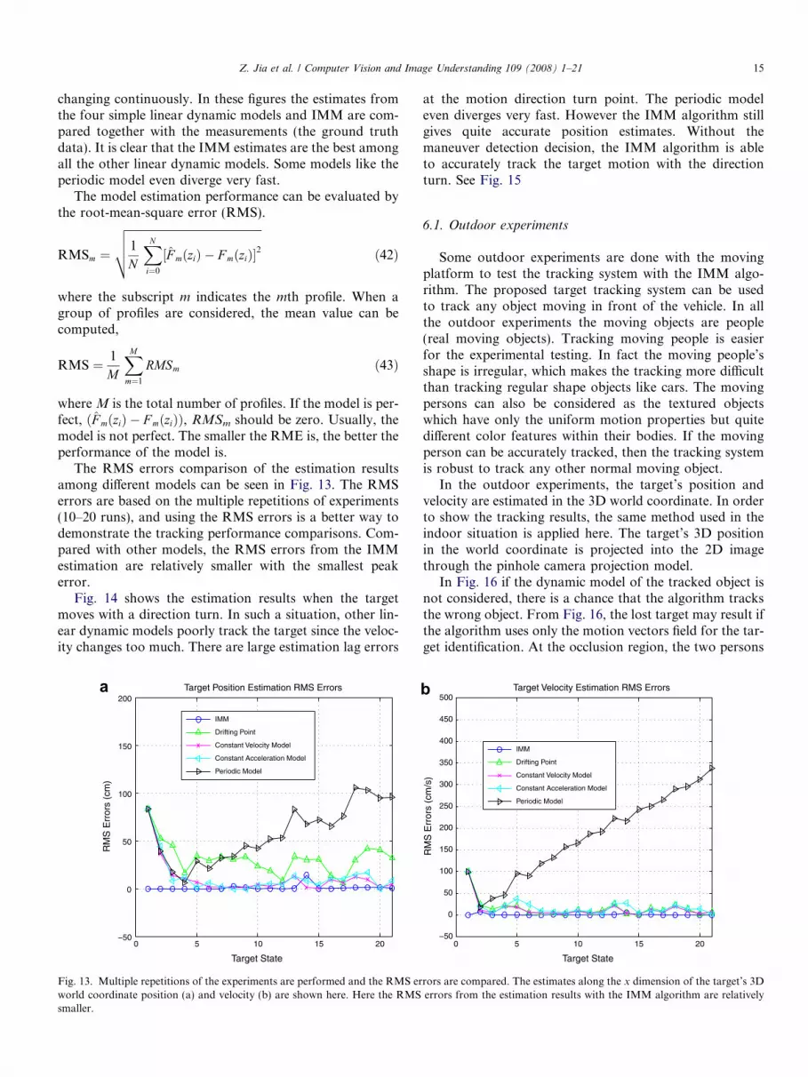
The RMS errors comparison of the estimation resultsamong different models can be seen in Fig. 13. The RMSerrors are based on the multiple repetitions of experiments(10–20 runs), and using the RMS errors is a better way todemonstrate the tracking performance comparisons. Com-pared with other models, the RMS errors from the IMMestimation are relatively smaller with the smallest peakerror.

Fig. 14 shows the estimation results when the targetmoves with a direction turn. In such a situation, other lin-ear dynamic models poorly track the target since the veloc-ity changes too much. There are large estimation lag errors

0 5 10 15 20

0

50

100

150

200Target Position Estimation RMS Errors

Target State

RM

S E

rror

s (c

m)

IMM

Drifting Point



Periodic Model

Fig. 13. Multiple repetitions of the experiments are performed and the RMS erworld coordinate position (a) and velocity (b) are shown here. Here the RMSsmaller.

at the motion direction turn point. The periodic modeleven diverges very fast. However the IMM algorithm stillgives quite accurate position estimates. Without themaneuver detection decision, the IMM algorithm is ableto accurately track the target motion with the directionturn. See Fig. 15

6.1. Outdoor experiments

Some outdoor experiments are done with the movingplatform to test the tracking system with the IMM algo-rithm. The proposed target tracking system can be usedto track any object moving in front of the vehicle. In allthe outdoor experiments the moving objects are people(real moving objects). Tracking moving people is easierfor the experimental testing. In fact the moving people’sshape is irregular, which makes the tracking more difficultthan tracking regular shape objects like cars. The movingpersons can also be considered as the textured objectswhich have only the uniform motion properties but quitedifferent color features within their bodies. If the movingperson can be accurately tracked, then the tracking systemis robust to track any other normal moving object.

In the outdoor experiments, the target’s position andvelocity are estimated in the 3D world coordinate. In orderto show the tracking results, the same method used in theindoor situation is applied here. The target’s 3D positionin the world coordinate is projected into the 2D imagethrough the pinhole camera projection model.

In Fig. 16 if the dynamic model of the tracked object isnot considered, there is a chance that the algorithm tracksthe wrong object. From Fig. 16, the lost target may result ifthe algorithm uses only the motion vectors field for the tar-get identification. At the occlusion region, the two persons

0 5 10 15 20

0

50

100

150

200

250

300

350

400

450

500Target Velocity Estimation RMS Errors

Target State

RM

S E

rror

s (c

m/s

)

IMM

Drifting Point



Periodic Model

rors are compared. The estimates along the x dimension of the target’s 3Derrors from the estimation results with the IMM algorithm are relatively

0 5 10 15 200

50

100

150

200

250

300

350

400Target Position Estimation Results

Target State

Pos

ition

(cm

)

Target Position Measurements

IMM

Drifting Point



Periodic Model

0 5 10 15 20

0

50

100Target Velocity Estimation Results

Target State

Vel

ocity

(cm

/s)

Target Velocity Measurements

IMM

Drifting Point



Periodic Model

a b

Fig. 14. Target dynamic information estimation results from different models with the target moving direction turn. The estimates along the x dimensionof the target’s 3D world coordinate position (a) and velocity (b) are shown here. In such a situation, the estimation results with the IMM algorithm are stillquite accurate. In these figures the target position measurements are the ground truth values.

0 5 10 15 20

0

50

100

150Target Position Estimation RMS Errors

Target State

RM

S E

rror

s (c

m)

IMM

Drifting Point



Periodic Model

0 5 10 15 20

0

50

100

150

200Target Velocity Estimation RMS Errors

Target State

RM

S E

rror

s (c

m/s

) IMM

Drifting Point



Periodic Model

Fig. 15. Multiple repetitions of the experiments are performed and the RMS errors are compared. The estimates along the x dimension of the target’s 3Dworld coordinate position (a) and velocity (b) are shown here. Here the RMS errors from the estimation results with the IMM algorithm are relativelysmaller.

Fig. 16. First, the person on the right is tracked. When these two people meet, due to occlusion the tracker will lose the target (a–e). The person movingfrom left to right is then tracked. (f) is the image segmentation result with occlusion. The tracking system can not recognize the previous tracked personwhen they are occluded.



have similar motion regions (Fig. 16f). The tracking algo-rithm can not distinguish the previous tracked one fromthe other.

In this paper, the above problem is solved by using asuitable dynamic model for tracking, which can estimateand predict the expected direction of the movement ofthe target. As explained earlier, the Interacting Multiplelinear dynamic Models algorithm is used to predict thenew possible position of the target in the image sequence.The predicted position of the target with its current posi-tion is used to identify the direction of its movement(Fig. 17). With the prediction, the above mentioned prob-lem is avoided as shown in Fig. 18.

In Fig. 19 two different persons are moving together inthe same direction and they have different velocities. Using

Fig. 17. Tracking with the direction prediction based on the dynamicmodel. The direction prediction can be used to solve the occlusionproblem.

Fig. 18. Improved tracking performance with the modifica

Fig. 19. Two persons are moving with a moving camera in a cluttered outdosecond person (d and e). The target is lost. Here the occlusion problem is solvedcan still be tracked.

Fig. 20. Target’s 3D tracking result when a person is interacting with the movinmoving towards the moving cameras. The person is correctly tracked with thchange between the person and the cameras.

the Extended Kalman Filter estimates, the tracked object’svelocity and motion direction can be estimated and thenonly in the predicted regions, the person is identified andtracked. In such a way, the previous tracked person is stillbeing correctly tracked.

Figs. 18, 20, 21 and 22 show the proposed algorithm’sperformance in different outdoor situations. First, themoving object can be seen as the textured object in theoutdoor cluttered environment. The moving person withdifferent colors within its body can be accurately segment-ed out and identified from the images using the fusionbased K-means clustering algorithm. Second, as the cam-eras and object are moving towards each other, the camer-as have not only the pure translational but also the 3Dmotions. Since the person’s moving region is required tobe in image scene for tracking, the target’s 3D velocityand position are estimated with the cameras’ rotationaland z-translational motions based on the moving cameras’kinematic model (R from Eq. (10) for the rotationalmotion and T from Eq. (11) for the translational motion).Third, in Fig. 20 the motion of the cameras looks largewhile in Fig. 21 the cameras look to be moving with a slowvelocity. When the moving cameras are moving close tothe moving object and their motion looks large, the chang-es between two consecutive images are relatively largerthan those with the cameras’ slow motion. In this paper,

tion to solve the two persons’ occlusion problem (a–e).

or environment (a–g). Here when the first person is fully occluded by thewith the Extended Kalman Filter prediction (Fig. 17) and the first person

g vehicle. The background is changing frame by frame (a–f). The person ise proposed system. The tracked region’s size is scaled due to the distance

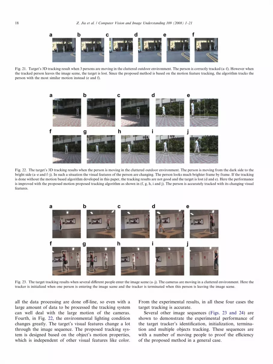
Fig. 21. Target’s 3D tracking result when 3 persons are moving in the cluttered outdoor environment. The person is correctly tracked (a–f). However whenthe tracked person leaves the image scene, the target is lost. Since the proposed method is based on the motion feature tracking, the algorithm tracks theperson with the most similar motion instead (e and f).

Fig. 22. The target’s 3D tracking results when the person is moving in the cluttered outdoor environment. The person is moving from the dark side to thebright side (a–e and f–j). In such a situation the visual features of the person are changing. The person looks much brighter frame by frame. If the trackingis done without the motion based algorithm developed in this paper, the tracking results are not good and the target is lost (d and e). Here the performanceis improved with the proposed motion proposed tracking algorithm as shown in (f, g, h, i and j). The person is accurately tracked with its changing visualfeatures.

Fig. 23. The target tracking results when several different people enter the image scene (a–j). The cameras are moving in a cluttered environment. Here thetracker is initialized when one person is entering the image scene and the tracker is terminated when this person is leaving the image scene.


all the data processing are done off-line, so even with alarge amount of data to be processed the tracking systemcan well deal with the large motion of the cameras.Fourth, in Fig. 22, the environmental lighting conditionchanges greatly. The target’s visual features change a lotthrough the image sequence. The proposed tracking sys-tem is designed based on the object’s motion properties,which is independent of other visual features like color.

From the experimental results, in all these four cases thetarget tracking is accurate.

Several other image sequences (Figs. 23 and 24) areshown to demonstrate the experimental performance ofthe target tracker’s identification, initialization, termina-tion and multiple objects tracking. These sequences arewith a number of moving people to proof the efficiencyof the proposed method in a general case.

Fig. 24. The target tracking results when several people are moving in the same environment (a–j). The cameras are also moving. As same as Fig. 23, thetracker can be automatically initialized and terminated for each person. The target tracking can be accurately done when several people move in the sameenvironment. Even if two persons have quite similar visual properties (h, i and j), the tracking can still be accurately done.


If a new person is entering the image scene, the trackercan be automatically identified and initialized for this per-son. When the person is leaving the image scene, the track-er can also be automatically terminated. The targettracking results are good as shown in Fig. 23.

In Figs. 23 and 24, the target tracking algorithm is testedwhen several different persons enter and leave the imagescene. In such a situation, the target tracking system cantrack different people at the same time in the same environ-ment. If several persons are moving in the environment anda new person is entering the image scene, the target track-ing is set so that the appearance of the pervious trackedperson is memorized as the image template, and then anew tracker different from the previous tracked one is ini-tialized for the newly entered motion region in the images.From the experimental results the system can accuratelyinitialize or terminate a tracker for each person. Thisreflects that the proposed target tracking algorithm hasthe ability to track different objects with similar visual fea-tures at the same time.

7. Conclusion

In this paper, a novel data fusion based target-trackingscheme is proposed. Optical flow vectors, stereo disparityand cameras’ motion parameters are combined togetherthrough the image processing algorithm to obtain the mov-ing target’s 3D dynamic features. Several simple and basiclinear dynamic models [13] are combined using the IMMalgorithm to provide an accurate approximate model forthe target’s dynamics. Through extensive experiments, theproposed tracking scheme demonstrates the advantagesof combining different data fusion strategies to get reliabletarget tracking results under different situations.

The main contribution of this paper is not any individ-ual technique used or developed but the whole new track-ing system formulated. In conclusion the proposedsystem has the following advantages over the previousworks such as [7,10,17,19, 20,26,33], 1. it is only based on

the vehicle’s onboard sensors to detect and track the object;2. the object is detected mainly based on its motion prop-erties independent of its specific visual properties, whichthus can deal with the situations of the unexpected or tex-tured objects tracking or tracking different objects at thesame environment. 3. the kinematic model of the vehicleis included in the tracking system, which can deal withthe cameras’ complex motions. 4. fusion of different track-ing models using IMM make target tracking more reliable.In conclusion it can be stated that the proposed trackingscheme is suitable for the target identification and trackingby autonomous vehicles.

The experiments in this paper are done off-line. Cur-rently, a moving platform is designed with all the sensorsand embedded pc available to simulate an autonomousvehicle. Building a real vehicle with fully autonomousfunctions is really difficult. But from the off-line outdoorexperiments, the results are good under different situa-tions and the theories of this paper are also sound. Soafter new hardwares are purchased and a whole newautonomous vehicle is built, the proposed algorithmscan be successfully implemented to get the satisfactoryreal-time performance. Another reason is that the real-time part of the experiments is only that after the targethas been tracked, the target’s dynamic information is justsent to the vehicle’s motion controller and it will generatecommands to control the vehicle’s movement to track orfollow the target. The vehicle’s kinematic control is reallyout of the scope of this paper. This paper is to design acomputer vision and sensor data fusion based targettracking system, and for this part it has successfully ful-filled the task.

The major computation complexity of the proposedscheme is from the image processing parts (optical flowvectors and stereo image processing). The 3D velocityestimation, the Extended Kalman Filter and the IMMalgorithm do not add any more computational burden.Thus in order to simplify the whole tracking system, theimage processing parts should be faster. However with


the rapid development of the hardware especially the imageprocessing cards (FPGA) available, in the future it is quitereasonable to make this tracking system perform well inreal-time.

As for future work, each part of the system can be mod-ified to make them work in cooperation under difficult sit-uations to get reliable results. These can be that: A betterimage segmentation algorithm and template initializingand updating algorithm can be developed to make theimage 2D features extractions more accurate. In order toobtain the best Extended Kalman Filter estimation results,the IMM algorithm has to be properly improved to meetthe following requirements: 1. design of the target motionmodels for all the modes of movements considering boththe quality and complexity of the model; 2. selection ofthe model parameters, such as the noise level. 3. determina-tion of the parameters of the underlying Markov chain,that is, the transition probabilities. Further experimentscan be done on autonomous vehicles to conduct the real-time target tracking tasks.

References

[1] Y. Bar-Shalom, X.R. Li, T. Kirubarajan, Estimation with Applica-tions to Tracking and Navigation, Wiley, New York, USA, 2001.

[2] J.L. Barron, D.J. Fleet, S.S. Beauchemin, Performance of optical flowtechniques, International Journal of Computer Vision 12 (1) (1994)43–77.

[3] C. Bregler. Learning and recognizing human dynamics in videosequences. In Proceedings of IEEE Computer Society Conference onComputer Vision and Pattern Recognition, San Juan, Puerto Rico,June 1997, pp. 568–574.

[4] T. Brox, A. Bruhn, N. Papenberg, J. Weickert. High accuracy opticalflow estimation based on a theory for warping. In Proceedings of 8thEuropean Conference on Computer Vision, volume 3024 of LectureNotes in Computer Science, Prague, Czech Republic, May 2004,Springer, pp. 25–36.

[5] J.Y. Chang, W.F. Hu, M.H. Cheng, B.S. Chang, Digital imagetranslational and rotational motion stabilization using optical flowtechnique, IEEE Transactions on Consumer Electronics 48 (1) (2002)108–115.

[6] D. Cremers, A variational framework for image segmentationcombining motion estimation and shape regularization. In Proceed-ings of 2003 IEEE Conference on Computer Vision and PatternRecognition, vol. 1, Madison, Wisconsin, USA, June 2003, pp.53–58.

[7] T. Dang, C. Hoffmann, C. Stiller. Fusing optical flow and stereodisparity for object tracking. In Proceedings of the 5th IEEEInternational Conference On Intelligent Transportation Systems,Singapore, September 2002, pp. 112–117.

[8] G.N. DeSouza, A.C. Kak, Vision for mobile robot navigation: Asurvey, IEEE Transactions on Pattern Analysis and Machine Intel-ligence 24 (2) (2002) 237–267.

[9] J.S. Evans, R.J. Evans, Image-enhanced multiple model tracking,Automatica 35 (11) (1999) 1769–1786.

[10] Y.J. Fang, I. Masaki, B. Horn, Depth-based target segmentation forintelligent vehicles: Fusion of radar and binocular stereo, IEEETransactions on Intelligent Transportation Systems 3 (2002) 196–202.

[11] M.E. Farmer, R.-L. Hsu, A.K. Jain, Interacting multiple model(imm) Kalman filters for robust high speed human motiontracking. In Proceedings of the 16th International Conference onPattern Recognition, vol. 2, pp. 20–23, Quebec City, Canada,August 2002.

[12] G. Farneback. Very high accuracy velocity estimation using orienta-tion tensors, parametric motion, and simultaneous segmentation ofthe motion field. In Proceedings of the Eighth IEEE InternationalConference on Computer Vision, vol. I, pp. 171–177, Vancouver,Canada, July 2001.

[13] D.A. Forsyth, J. Ponce, Computer Vision: A Modern Approach,Prentice Hall, USA, 2002.

[14] B.K.P. Horn, Robot Vision, MIT Press, USA, 1986.[15] W.M. Hu, T.N. Tan, L. Wang, S. Maybank, A survey on visual

surveillance of object motion and behaviors, IEEE Transactions onSystems, Man, and Cybernetics—Part C: Applications and Reviews34 (3) (2004) 334–352.

[16] M.H. Jeong, Y. Kuno, N. Shimada, Y. Shirai. Two-hand gesturerecognition using coupled switching linear model. In Proceedings ofthe 16th International Conference on Pattern Recognition, vol. 3, pp.529–532, Quebec City, Canada, August 2002.

[17] Zhen Jia, A. Balasuriya, S. Challa. Motion based 3d target trackingwith interacting multiple linear dynamic models. In Proceedings ofthe 15th British Machine Vision Conference, United Kindom,September 2004.

[18] Zhen Jia, A. Balasuriya, and S. Challa. Visual information andcamera motion fusion for 3d target tracking. In Proceedings ofThe Eighth International Conference on Control, Automation,Robotics and Vision, pp. 2296–2301, Kunming, China, December2004.

[19] Zhen Jia, A. Balasuriya, S. Challa. Sensor fusion based 3d targetvisual tracking for autonomous vehicles with imm. In Proceedings of2005 IEEE International Conference on Robotics and Automation(ICRA 2005), Barcelona, Spain, April 2005, pp. 1841–1846.

[20] A. Kosaka, M. Meng, and A.C. Kak. Vision-guided mobile robotnavigation using retroactive updating of position uncertainty. InProceedings of 1993 IEEE International Conference on Robotics andAutomation, vol. 2, Atlanta, Georgia, USA, May 1993, pp. 1–7.

[21] F. Liu, X.Y. Lin, S.Z. Li, Y. Shi. Multi-modal face tracking usingBayesian network. In Proceedings of IEEE International Workshopon Analysis and Modelling of Faces and Gestures, Nice, France,October 2003, pp. 135–142.

[22] I. Matthews, T. Ishikawaa, S. Baker, The template update problem,IEEE Transactions on Pattern Analysis and Machine Intelligence 26(6) (2004) 810–815.

[23] K. Morioka, J.H. Lee, H. Hashimoto, Human-following mobilerobot in a distributed intelligent sensor network, IEEE Transactionson Industrial Electronics 51 (1) (2004) 229–237.

[24] K. Muhlmann, D. Maier, R. Hesser, R. Manner. Calculating densedisparity maps from color stereo images, an efficient implementation.In Proceedings of the IEEE Workshop on Stereo and Multi-BaselineVision, Kauai, Hawaii, USA, December 2001, pp. 30–36.

[25] S. Nadimi, B. Bhanu. Multistrategy fusion using mixture model formoving object detection. In Proceedings of International Conferenceon Multisensor Fusion and Integration for Intelligent Systems,Baden-Baden, German, August 2001, pp. 317–322.

[26] R. Okada, Y. Shirai, and J. Miura. Tracking a person with 3-dmotion by integrating optical flow and depth. In Proceedings ofthe Fourth IEEE International Conference on Automatic Faceand Gesture Recognition, Grenoble, France, March 2000, pp. 336–341.

[27] V. Pavlovic, J.M. Rehg, T.J. Cham, and K.P. Murphy. A dynamicbayesian network approach to figure tracking using learned dynam-ical models. In Proceedings of International Conference on ComputerVision, Kerkyra, Corfu, Greece, September 1999, pp. 94–101.

[28] N. Peterfreund, Robust tracking of position and velocity withKalman snakes, IEEE Transactions on Pattern Analysis and MachineIntelligence 21 (6) (1999) 564–569.

[29] S. Ray, R. H. Turi. Determination of number of clusters in k-meansclustering and application in colour image segmentation. In Proceed-ings of the 4th International Conference on Advances in PatternRecognition and Digital Techniques (ICAPRDT’99), Calcutta, India,December 1999, pp. 137–143.


[30] M. Ridley, E. Nettleton, S. Sukkarieh, H. Durrant-Whyte. Trackingin decentralised air-ground sensing networks. In Proceedings of theFifth International Conference on Information Fusion, vol. 1,Annapolis, USA, July 2002, pp. 616–623,.

[31] D. Wettergreen, C. Gaskett, and A. Zelinsky. Development ofa visually-guided autonomous underwater vehicle. In Proceedingsof Conference on OCEANS, vol. 2, September 1998, pp. 1200–1204.

[32] T. Yamane, Y. Shirai, J. Miura. Person tracking by integratingoptical flow and uniform brightness regions. In Proceedings of IEEEInternational Conference on Robotics and Automation, vol. 4,Leuven, Belgium, May 1998, pp. 3267–3272.

[33] F. Yang and A. Balasuriya. Optical flow based speed estimation inauv target tracking. In Proceedings of MTS/IEEE Conference andExhibition on OCEANS, vol. 4, Hawaii, USA, November, pp. 2377–2382.

vision based data fusion for autonomous vehicles target tracking using interacting multiple dynamic...

Documents