very sparse lssvm reductions for large scale data - ku
TRANSCRIPT
1
Very Sparse LSSVM Reductions for Large ScaleData
Raghvendra Mall and Johan A.K. Suykens
Abstract—Least Squares Support Vector Machines (LSSVM)have been widely applied for classification and regression withcomparable performance to SVMs. The LSSVM model lackssparsity and is unable to handle large scale data due to compu-tational and memory constraints. A primal Fixed-Size LSSVM(PFS-LSSVM) was previously proposed in [1] to introducesparsity using Nystrom approximation with a set of prototypevectors (PV). The PFS-LSSVM model solves an over-determinedsystem of linear equations in the primal. However, this solutionis not the sparsest. We investigate the sparsity-error trade-off byintroducing a second level of sparsity. This is done by meansof L0-norm based reductions by iteratively sparsifying LSSVMand PFS-LSSVM models. The exact choice of the cardinality forthe initial PV set is not important then as the final model ishighly sparse. The proposed method overcomes the problem ofmemory constraints and high computational costs resulting inhighly sparse reductions to LSSVM models. The approximationsof the two models allow to scale the models to large scale datasets.Experiments on real world classification and regression datasetsfrom the UCI repository illustrate that these approaches achievesparse models without a significant trade-off in errors.
Index Terms—L0-norm, reduced models, LSSVM classification& regression, sparsity
I. INTRODUCTION
Least Squares Support Vector Machines (LSSVM) wereintroduced in [2] and have become a state-of-the-art learningtechnique for classification and regression. In the LSSVM for-mulation instead of solving a quadratic programming problemwith inequality constraints as in the standard SVM [3], one hasequality constraints and the L2-loss function. This leads to anoptimization problem whose solution in the dual is obtainedby solving a system of linear equations.
A drawback of LSSVM models is the lack of sparsity asusually all the data points become support vectors (SV) asshown in [1]. Several works in the literature address thisproblem of lack of sparsity in the LSSVM model. They canbe categorized as:
1) Reduction methods: - Training the model on the dataset,pruning support vectors and selecting the rest for retrain-ing the model.
2) Direct methods: - Enforcing sparsity from the beginning.Some works in the first category are [4], [5], [6], [7], [8], [11],[9] and [10]. In [5], the authors provide an approximate SVMsolution under the assumption that the classification problem
Raghvendra Mall, Department of Electrical Engineering, ESAT-STADIUS (SCD), KU Leuven, B-3001 Leuven, Belgium, email:[email protected].
Johan A.K. Suykens, Department of Electrical Engineering,ESAT-STADIUS (SCD), KU Leuven, B-3001 Leuven, Belgium,email:[email protected].
is separable in the feature space. In [6] and [7], the proposedalgorithm approximates the weight vector such that the dis-tance to the original weight vector is minimized. The authorsof [8] eliminate the support vectors that are linearly dependenton other support vectors. In [9] and [10], the authors work ona reduced set for optimization by pre-selecting a subset of dataas support vectors without emphasizing much on the selectionmethodology. The authors of [11] prune the support vectorswhich are farthest from the decision boundary. This is donerecursively until the performance degrades. Another work [12]in this direction suggests to select the support vectors closerto the decision boundary. However, these techniques cannotguarantee a large reduction in the number of support vectors.
In the second category, the number of support vectors re-ferred to as prototype vectors (PVs) are fixed in advance. Onesuch approach is introduced in [1] and is referred to as fixed-size least squares support vector machines (FS-LSSVM). Itprovides a solution to the LSSVM problem in the primal spaceresulting in a parametric model and a sparse representation.The method uses an explicit expression for the feature mapusing the Nystrom method [13] and [14]. The Nystrom methodis related to finding a low rank approximation to the givenkernel matrix by choosing M rows or columns from the largeN ×N kernel matrix. In [1], the authors proposed searchingfor M rows or columns by maximizing the quadratic Renyientropy criterion. It was shown in [15] that the cross-validationerror of primal FS-LSSVM (PFS-LSSVM) decreases withrespect to the number of selected PVs until it does not changeanymore and is heavily dependent on the initial set of PVsselected by quadratic Renyi entropy. This point of “saturation”can be achieved for M ¿ N but this is not the sparsestsolution. A sparse conjugate direction pursuit approach wasdeveloped in [16] where they iteratively build up a conjugateset of vectors of increasing cardinality to approximately solvethe over-determined PFS-LSSVM linear system. The approachworks most efficiently when few iterations suffice for a goodapproximation. However, when few iterations don’t suffice forapproximating the solution the cardinality will be M .
In recent years the L0-norm has been receiving increasingattention. The L0-norm is the number of non-zero elementsof a vector. So when the L0-norm of a vector is minimizedit results into the sparsest model. But this problem is NP-hard. Therefore, several approximations to it are discussedin [17] and [18] etc. In this paper, we modify the iterativesparsification procedure introduced in [19] and [20]. The majordrawbacks of the methods described in [19] and [20] are thatthese approaches cannot scale to very large scale datasets dueto memory (N×N kernel matrix) and computational (O(N3)
2
time) constraints. We reformulate the iterative sparsificationprocedure for LSSVM and PFS-LSSVM methods to producehighly sparse models. These models can efficiently handlevery large scale data. We discuss two different initializationmethods for which in a next step the sparsification step isapplied:• Initialization by Primal Fixed-Size LSSVM: Sparsifi-
cation of the primal fixed-size LSSVM (PFS-LSSVM)method leads to a highly sparse parametric model namelysparsified primal FS-LSSVM (SPFS-LSSVM).
• Initialization by Subsampled Dual LSSVM: The subsam-pled dual LSSVM (SD-LSSVM) is a fast initialization tothe LSSVM model solved in the dual. Its sparsificationresults into a highly sparse non-parametric model namelysparsified subsampled dual LSSVM (SSD-LSSVM).
We compare the proposed methods with state-of-the-arttechniques including C-SV C, ν-SV C from the LIBSVM[22] software, Keerthi’s method [23], L0-norm based methodproposed by Lopez [20] and the L0-reduced PFS-LSSVMmethod (SV L0-norm PFS-LSSVM) [21] on several bench-mark datasets from the UCI repository [24]. Below we mentionsome motivations to obtain a sparse solution:• Sparseness can be exploited for having more memory
and computationally efficient techniques, e.g. in matrixmultiplications and inversions.
• Sparseness is essential for practical purposes such asscaling the algorithm to very large scale datasets. Sparsesolutions means fewer support vectors and less timerequired for out-of-sample extensions.
• By introducing two levels of sparsity, we overcome theproblem of selection of the smallest cardinality (M ) forthe PV set faced by the PFS-LSSVM method.
• The two level of sparsity allows scaling to large scaledatasets while having very sparse models.
We also investigate the sparsity versus error trade-off.This paper is organized as follows. A brief description of
PFS-LSSVM and SD-LSSVM is given in Section II. The L0-norm based reductions to PFS-LSSVM, i.e., SPFS-LSSVMand SD-LSSVM, i.e., SSD-LSSVM are discussed in SectionIII. In Section IV, the different algorithms are successfullydemonstrated on real-life datasets. We discuss about the spar-sity versus error trade-off in Section V. Section VI states theconclusion of the paper.
II. INITIALIZATIONS
In this paper, we consider two initializations. One is basedon solving the least squares support vector machine problemin the primal (PFS-LSSVM). The other is a fast initializationmethod solving a subsampled least squares support vectormachines problem in the dual (SD-LSSVM).
A. Primal FS-LSSVM
1) Least Squares Support Vector Machine: We provide abrief summary of the Least Squares Support Vector Machines(LSSVM) methodology for classification and regression.
Given a sample of N data points xi, yi, i = 1, ..., N,where xi ∈ Rd and yi ∈ +1,−1 for classification and yi ∈
R for regression, the LSSVM primal problem is formulatedas follows:
minw,b,e
J (w, e) =12wᵀw +
γ
2
N∑
i=1
e2i
s.t. wᵀφ(xi) + b = yi − ei, i = 1, . . . , N,
(1)
where φ : Rd → Rnh is a feature map to a high dimensionalfeature space, where nh denotes the dimension of the featurespace (which can be infinite dimensional), ei ∈ R are theerrors and w ∈ Rnh , b ∈ R.
Using the coefficients αi for the Lagrange multipliers, thesolution to (1) can be obtained by the Karush-Kuhn-Tucker(KKT) [25] conditions for optimality. The result is given bythe following linear system in the dual variables αi:
[0 1ᵀ
N
1N Ω + 1γ IN
] [bα
]=
[0y
], (2)
with y = (y1, y2, . . . , yN )ᵀ, 1N = (1, . . . , 1)ᵀ, α =(α1, α2, . . . , αN )ᵀ and Ωkl = φ(xk)ᵀφ(xl) = K(xk, xl), fork, l = 1, . . . , N with K a Mercer kernel function. From the
KKT conditions we get that w =N∑
i=1
αiφ(xi) and αi = γei.
The second condition causes the LSSVM to be non-sparse aswhenever ei is non-zero then αi 6= 0. Generally, in real worldscenarios the ei 6= 0, i = 1, . . . , N for most data points. Thisleads to lack of sparsity in the LSSVM model.
2) Nystrom Approximation and Primal Estimation: Forlarge datasets it is often advantageous to solve the problemin the primal where the dimension of the parameter vectorw ∈ Rd is smaller compared to α ∈ RN . However, oneneeds an explicit expression for φ or the approximation ofthe nonlinear mapping φ : Rd → RM based on a sampledset of prototype vectors (PV) from the whole dataset. In [15],the authors provide a method to select this subsample of sizeM ¿ N by maximizing the Quadratic Renyi entropy.
Williams and Seeger [26] uses the Nystrom method tocompute the approximated feature map φ : Rd → RM , i =1, . . . ,M for a training point, or for any new point x∗, withφ = (φ1, . . . , φM )ᵀ, is given by
φi(x∗) =1√λs
i
M∑
j=1
(ui)jK(zj , x∗), (3)
where λsi and ui denote the eigenvalues and the eigenvectors of
the kernel matrix Ω ∈ RM×M with Ωij = K(zi, zj), where zi
and zj belong to the subsampled set SPV which is a subset ofthe whole dataset D. The matrix Ω relates to a subset of the bigkernel matrix Ω ∈ RN×N . However, we should never calculatethis big kernel matrix Ω in our proposed methodologies. Thecomputation of the features corresponding to each point xi ∈D in matrix notation can be written as:
Φ =
φ1(x1) . . . φM (x1)...
. . ....
φ1(xN ) . . . φM (xN )
. (4)
Solving (1) with the approximate feature matrix Φ ∈ RN×M
in the primal as proposed in [1] results into solving the
3
following linear system of equations:[
ΦᵀΦ + 1γ I Φᵀ1N
1ᵀN Φ 1ᵀ
N1N
] [w
b
]=
[Φᵀy1ᵀ
Ny
], (5)
where w ∈ RM , b ∈ R are the model parameters in the primalspace with y ∈ +1,−1 for classification and y ∈ R forregression.
3) Parameter Estimation for Very Large Datasets: In [15],the authors propose a technique to obtain tuning parametersfor very large scale datasets. We utilize the same methodologyto obtain the parameters of the model (w and b) when theapproximate feature matrix Φ given by (4) cannot fit intomemory. The basic concept is to decompose the feature matrixΦ into a set of S blocks. Thus, Φ is not required to be storedinto memory completely. Let ls, where s = 1, . . . , S, denote
the number of rows in the sth block such thatS∑
s=1ls = N .
The matrix Φ can be described as:
Φ =
Φ[1]
...Φ[S]
,
with Φ[S] ∈ Rls×(M+1) and the vector y is given by
y =
y[1]
...y[S]
,
with y[S] ∈ Rls . The matrix Φᵀ[S]Φ[S] and the vector Φᵀ
[S]y[S]
can be calculated in an updating scheme and stored efficientlyin the memory since their sizes are (M + 1) × (M + 1) and(M +1)×1 respectively, provided that the size of each block,i.e., ls can fit into memory. Moreover, the following also holds:
ΦᵀΦ =S∑
s=1
Φᵀ[s]Φ[s], Φᵀy =
S∑s=1
Φᵀ[s]y[s].
Algorithm 1 summarizes the overall idea.
Algorithm 1: PFS-LSSVM for very large scale data [15]Divide the training data D into approximately S equal blockssuch that Φ[s] with s = 1, . . . , S, calculated using (4) can fitinto memory.Initialize matrix A ∈ R(M+1)×(M+1) and c ∈ RM+1.for s = 1 to S do
Calculate matrix Φ[s] for the sth block using Nystromapproximation (4)A← A + Φᵀ
[s]Φ[s]
c← c + Φᵀ[s]y[s]
endSet A← A +
IM+1γ
Solve the linear system (5) to obtain parameters w,b.
Algorithm 2: Primal FS-LSSVM methodData: D = (xi, yi) : xi ∈ Rd, yi ∈ +1,−1 for
classification & yi ∈ R for regression, i = 1, . . . , N.1 Determine the kernel bandwidth using the multivariate
rule-of-thumb.2 Given the number of PV, perform prototype vector selection by
maximizing the quadratic Renyi entropy.3 Determine the learning parameters σ and γ performing fast
v-fold cross validation as described in [15].4 if the approximate feature matrix (4) can be stored into
memory then5 Given the optimal learning parameters, obtain the
PFS-LSSVM parameters w and b by solving the linearequation (5).
6 else7 Use Algorithm 1 to obtain the PFS-LSSVM parameters w
and b.8 end
B. Fast Initialization: Subsampled Dual LSSVM
In this case, we propose a different approximation instead ofthe Nystrom approximation and solve a subsampled LSSVMproblem in the dual (SD-LSSVM). We first use the activesubset selection method as described in [15] to obtain an initialset of prototype vectors PV, i.e., SPV . This set of points isobtained by maximizing the quadratic Renyi entropy criterion,i.e., approximate the information of the big N × N kernelmatrix by means of a smaller M ×M matrix and this can beconsidered as the set of representative points of the dataset.
The assumption for the approximation in the proposedapproach is that this set of prototype vectors is sufficient totrain an initial LSSVM model in the dual and is sufficientto obtain the tuning parameters σ and γ for the SD-LSSVMmodel. Here the major advantage is that it greatly reducesthe computation time required for training and cross-validation(O(M3) in comparison to O(NM2) for PFS-LSSVM). Thisresults in an approximate value for the tuning parameters closeto the optimal values (for the entire training dataset). However,as the training of the LSSVM model is performed in the dual,we no longer need explicit approximate feature maps and canhave the original feature map of the form φ : Rd → Rnh
where nh denotes the dimension of the feature space whichcan be infinite dimensional.
Thus, the SD-LSSVM problem of training on the M pro-totype vectors selected by Renyi entropy is given by:
minw,b,e
J (w, e) =12wᵀw +
γ
2
M∑
i=1
e2i
s.t. wᵀφ(zi) + b = yi − ei, i = 1, . . . , M,
(6)
where zi ∈ SPV and SPV is a subset of the whole dataset D.
III. SPARSIFICATIONS
We propose two L0-norm reduced models starting fromthe initializations explained in Section II: One for the primalFS-LSSVM method namely the sparsified primal FS-LSSVM(SPFS-LSSVM) and the other one for the SD-LSSVM methodnamely sparsified subsampled dual LSSVM (SSD-LSSVM).Both models can handle very large scale data efficiently.
4
A. L0-norm Reduced PFS-LSSVM - SPFS-LSSVM
In this section, we propose an approach using the L0-normto introduce a second level of sparsity resulting in a reducedset of prototype vectors SSV whose cardinality is M ′ andis giving a highly sparse solution. We modify the proceduredescribed in [19] and [20]. The methodology used in [19] and[20] cannot be extended to large scale data due to memoryconstraints (O(N × N)) and computational costs (O(N3)).The L0-norm problem can be formulated as:
minw,b,e
J (w, e) = ‖w‖0 +γ
2
N∑
i=1
e2i
s.t. wᵀφ(xi) + b = yi − ei, i = 1, . . . , N,
(7)
where w, b and ei, i = 1, . . . , N are the variables of theoptimization problem and φ is the explicit feature map asdiscussed in (3).
The weight vector w can be approximated as a linear com-bination of the M prototype vectors, i.e., w =
∑Mj=1 βj φ(zj)
where βj ∈ R which don’t need to be the Lagrange multipliers.We apply the regularization weight λj on each of these βj
to iteratively sparsify such that most of the βj move to zeroleading to an approximate L0-norm solution as shown in [19].The L0-norm problem can then be re-formulated in terms ofreweighting steps of the form:
minβ,b,e
J(β, e) =12
M∑
j=1
λj β2j +
γ
2
N∑
i=1
e2i
s.t.M∑
j
βjQij + b = yi − ei, i = 1, . . . , N.
(8)
The matrix Q is a rectangular matrix of size N ×M and isdefined by its elements Qij = φ(xi)ᵀφ(zj) where xi ∈ D,zj ∈ SPV . The set SPV is a subset of the dataset D. Thisproblem (8) is similar to the one formulated for SVMs in [19]and guarantees sparsity and convergence. It is well knownthat the Lp-norm problem is non-convex for 0 < p < 1. Weobtain an approximate solution for p → 0 by the iterativesparsification procedure and converge to a local minimum.
We propose to solve this problem in the primal whichallows us to extend the sparsification procedure to large scaledatasets along with incorporating the information about theentire training dataset D. Thus, after eliminating the ei theoptimization problem becomes:
minβ,b
J(β, b) =12
M∑
j=1
λj β2j +
γ
2
N∑
i=1
(yi − (M∑
j=1
βjQij + b))2.
(9)The solution to (9) resembles the ridge regression solution
(in case of zero bias term) and is obtained by solving:[
QᵀQ + 1γ diag(λ) Qᵀ1N
1ᵀN Q 1ᵀ
N1N
][β
b
]=
[Qᵀy1ᵀ
Ny
](10)
where diag(λ) is a diagonal M × M matrix with diagonalelements λj . The iterative sparsification method is presentedin Algorithm 3.
Algorithm 3: SPFS-LSSVM method
Data: Solve PFS-LSSVM (5) to obtain initial w and bβ = wλi ← βi, i = 1, . . . , Mif the Q matrix can be stored into memory then
Calculate QᵀQ once and store into memory.else
Divide into blocks for very large datasets computingQᵀ
[s]Q[s] in an additive updating scheme similar toprocedure in Algorithm 1.Calculate once and store the M ×M matrix into memory.
endwhile not convergence do
H ← QᵀQ + diag(λ)/γ ;Solve system (10) to give β and b ;λi ← 1/β2
i , i = 1, . . . , M ;endResult: indices = find(|βi| > 0), β′ = β(indices), b′ = b.
The procedure to obtain sparseness involves iteratively solv-ing the system (10) for decreasing values of λ. Considering thetth iteration, we can build the matrix H ← QᵀQ+diag(λ)/γfrom the in-memory matrix QᵀQ and the modified matrixdiag(λt) and solve the system of linear equations. From thissolution we get λt+1 and the process is restarted. It was shownin [19] that as t→∞, βt converges to the L0-norm solutionasymptotically. This is shown in Algorithm 3. Since, this β′
depends on the initial choice of weights, we set them to thePFS-LSSVM solution w and b to avoid ending up in verydifferent local minima. For this procedure we need to calculateQᵀQ matrix just once and keep it into memory. The finalpredictive model is:
f(x∗) =M ′∑
i=1
β′iφ(zi)ᵀφ(x∗) + b′.
We use f(x∗) for regression and sign[f(x∗)] for classification.Table I provides a conceptual and notational overview of thesteps involved in SPFS-LSSVM model.
Initial 1st Reduction 2nd ReductionSV/Train N/N M/N M ′/N
Primal w, D Step 1 → w, SPV Step 2 → β′, b′, SSVφ(x) ∈ Rnh PFS-LSSVM φ(x) ∈ RM SPFS-LSSVM
TABLE I: Given the dataset D we first perform the primal FS-LSSVM in Step 1. We obtain the prototype vector set SPV , theweight vector w along with the explicit feature map φ : Rd →RM . In Step 2 we perform the SPFS-LSSVM, i.e., we use aniterative sparsifying L0-norm procedure in the primal wherew =
∑Mj=1 βj φ(zj) and regularization weights λj are applied
on βj . We construct the Q matrix which has information aboutthe entire training set D. After the 2nd reduction we obtainthe solution vector β′ and b′. The solution vector relates toprototype vectors of the highly sparse solution set SSV .
5
B. L0-norm reduced subsampled dual LSSVM - SSD-LSSVM
The subsampled dual LSSVM (SD-LSSVM) performs afast initialization on a subsample obtained by maximizing thequadratic Renyi entropy. The SD-LSSVM model as describedin Section II results in α, i = 1, . . . , M and b as a solutionin the dual. However, we have not seen all the data in thetraining set for this case. Also, we don’t know beforehandthe ideal value of the cardinality M for the initial PV set.In general, we start with a large value of M for fixing theinitial cardinality of the PV set. But we propose an iterativesparsification procedure for the SD-LSSVM model leading toan L0-norm based solution. This results in a set of reducedprototype vectors SSV whose cardinality is M ′ which can bemuch less than M . We use these reduced prototype vectorsalong with the non-zero αi, i = 1, . . . , M and b obtained asa result of the iterative sparsification procedure for the out-of-sample extensions (i.e. test data predictions). The L0-normproblem for the SD-LSSVM model can then be formulated as:
minw,b,e
J (w, e) = ‖w‖0 +γ
2
N∑
i=1
e2i
s.t. wᵀφ(xi) + b = yi − ei, i = 1, . . . , N,
(11)
where w, b and ei, i = 1, . . . , N are the variables of theoptimization problem and φ is the original feature map.
One of the KKT conditions of (6) is w =M∑i=1
αiφ(zi) where
αi are Lagrange dual variables. We apply the regularizationweight λj on each of these αj to iteratively sparsify such thatmost of the αj move to zero leading to an approximate L0-norm solution as shown in [19]. In order to handle large scaledatasets and obtain the non-zero αj leading to the reducedset of prototype vectors SSV , we formulate the optimizationproblem by eliminating each ei. Thus, the optimization prob-lem can be reformulated as:
minα,b
J(α, b) =12
M∑
j=1
λjα2j +
γ
2
N∑
i=1
(yi − (M∑
j=1
αjQij + b))2.
(12)The matrix Q is a rectangular matrix of size N × M andis defined by its elements Qij = φ(xi)ᵀφ(zj) = K(xi, zj)where xi ∈ D, zj ∈ SPV . The variables xj and zj which arepart of the PV set SPV are used interchangeably. This marksthe distinction between (12) and (9) where we use explicitapproximate feature maps. The solution to (12) is obtained bysolving:
[QᵀQ + 1
γ diag(λ) Qᵀ1N
1ᵀNQ 1ᵀ
N1N
] [αb
]=
[Qᵀy1ᵀ
Ny
]. (13)
Here diag(λ) is a diagonal M × M matrix with diagonalelements λj . We train the SD-LSSVM only on the PV set(cardinality M ) but we incorporate the information from theentire training dataset (cardinality N ) in the loss functionwhile performing the iterative sparsification algorithm. Thisresults into an improvement in performance as more informa-tion is incorporated in the model. The approach to perform aniterative sparsification procedure for the SD-LSSVM model ispresented in Algorithm 4.
Algorithm 4: SSD-LSSVM methodData: Solve SD-LSSVM (6) on actively selected PV set to
obtain the initial α and bλi ← αi, i = 1, . . . , Mif the Q matrix can be stored into memory then
Calculate QᵀQ once and store into memory.else
Divide into blocks for very large datasets computingQᵀ
[s]Q[s] in an additive updating scheme similar toprocedure in Algorithm 1.Calculate once and store the M ×M matrix into memory.
endwhile not convergence do
H ← QᵀQ + diag(λ)/γ ;Solve system (13) to give α and b ;λi ← 1/α2
i , i = 1, . . . , M ;endResult: indices = find(|αi| > 0), α′ = α(indices), b′ = b
The procedure to obtain sparseness works similarly asdescribed in Section III-A. Once we obtain the indicescorresponding to the non-zero αi, we can obtain the reducedset of prototype vectors SV corresponding to those non-zeroαi. We can then use α′ and b′ (as defined in Algorithm 4)along with these SV to perform the test predictions. The finalpredictive model is:
f(x∗) =M ′∑
i=1
α′iK(zi, x∗) + b′.
We use f(x∗) for regression and sign[f(x∗)] for classification.Table II provides a conceptual and notational overview of thesteps involved in SSD-LSSVM model.
Initial 1st Reduction 2nd ReductionSV/Train N/N M/M M ′/N
Dual α, D Step 1 → α, SP V Step 2 → α′, b′, SSV
φ(x) ∈ Rnh SD-LSSVM φ(x) ∈ Rnh SSD-LSSVM
TABLE II: Given the dataset D we first perform the SD-LSSVM as a fast initialization in Step 1. We obtain the dualLagrange variables αi, i = 1, . . . , M . In Step 2 we performthe SSD-LSSVM, i.e., we use an iterative sparsifying L0-norm procedure in the primal resulting in a reduced set ofvectors SSV . We construct the rectangular matrix Q whichincorporates information about the entire training set. Afterthe 2nd reduction we select the non-zero αi and b to obtainthe solution vector α′ and b′.
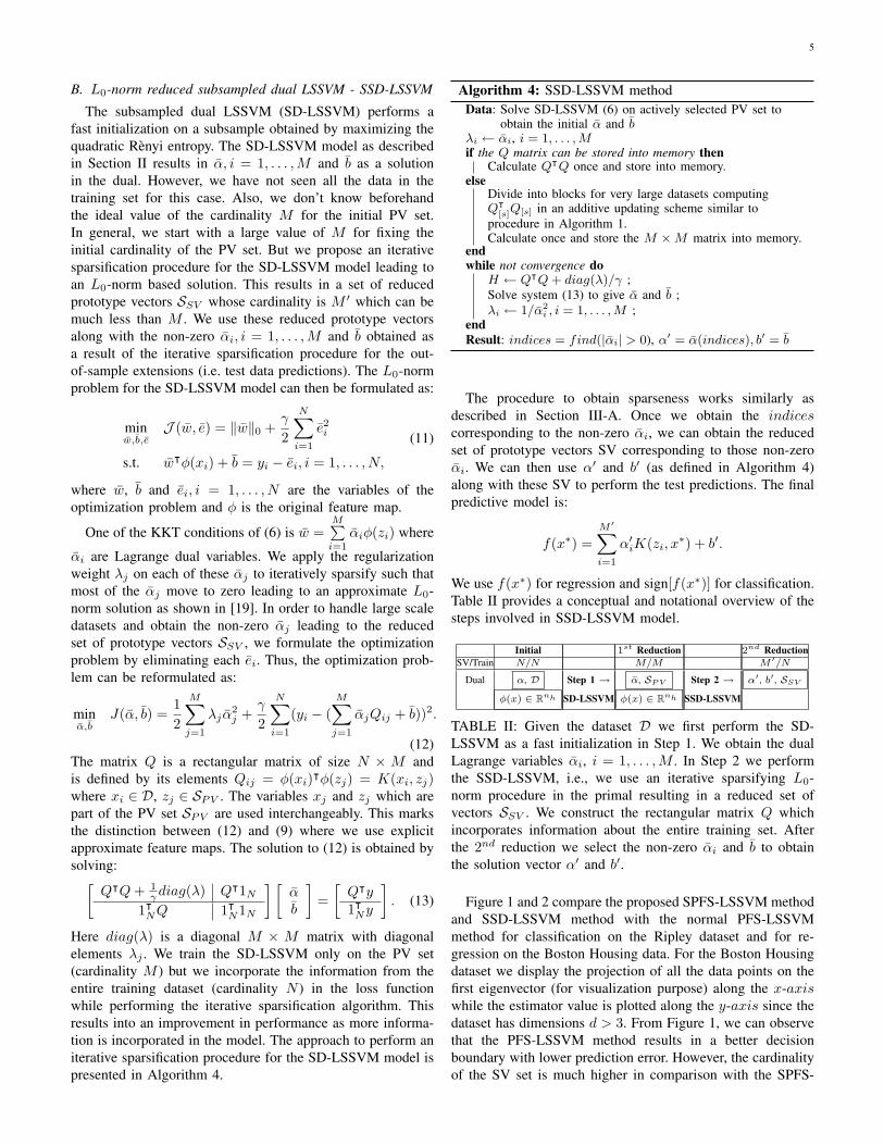
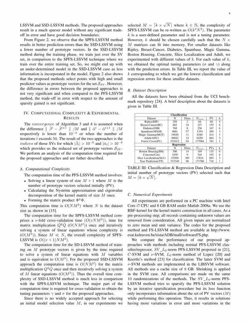
Figure 1 and 2 compare the proposed SPFS-LSSVM methodand SSD-LSSVM method with the normal PFS-LSSVMmethod for classification on the Ripley dataset and for re-gression on the Boston Housing data. For the Boston Housingdataset we display the projection of all the data points on thefirst eigenvector (for visualization purpose) along the x-axiswhile the estimator value is plotted along the y-axis since thedataset has dimensions d > 3. From Figure 1, we can observethat the PFS-LSSVM method results in a better decisionboundary with lower prediction error. However, the cardinalityof the SV set is much higher in comparison with the SPFS-
6
LSSVM and SSD-LSSVM methods. The proposed approachesresult in a much sparser model without any significant trade-off in error and have good decision boundaries.
From Figure 2, we observe that the SPFS-LSSVM methodresults in better prediction errors than the SSD-LSSVM usinga fewer number of prototype vectors. In the SSD-LSSVMmethod during the training phase, we train just over the SVset, in comparison to the SPFS-LSSVM technique where wetrain over the entire training set. So, we might end up withan under-determined model in the SSD-LSSVM case as lessinformation is incorporated in the model. Figure 2 also showsthat the proposed methods select points with high and smallpredictor values as prototype vectors for the set SSV . However,the difference in errors between the proposed approaches isnot very significant and when compared to the PFS-LSSVMmethod, the trade-off in error with respect to the amount ofsparsity gained is not significant.
IV. COMPUTATIONAL COMPLEXITY & EXPERIMENTALRESULTS
The convergence of Algorithm 3 and 4 is assumed whenthe difference ‖ βt − βt+1 ‖ /M and ‖ αt − αt+1 ‖ /Mrespectively is lower than 10−4 or when the number ofiterations t exceeds 50. The result of the two approaches is theindices of those SVs for which |βi| > 10−6 and |αi| > 10−6
which provides us the reduced set of prototype vectors SSV .We perform an analysis of the computation time required forthe proposed approaches and are futher described.
A. Computational Complexity
The computation time of the PFS-LSSVM method involves:• Solving a linear system of size M + 1 where M is the
number of prototype vectors selected initially (PV).• Calculating the Nystrom approximation and eigenvalue
decomposition of the kernel matrix of size M once.• Forming the matrix product ΦᵀΦ.
This computation time is O(NM2) where N is the datasetsize as shown in [15].
The computation time for the SPFS-LSSVM method com-prises a v-fold cross-validation time (O(vNM2)), time formatrix multiplication QᵀQ (O(NM2)) once and iterativelysolving a system of linear equations whose complexity is(O(M3)). Since M ¿ N , the overall complexity of SPFS-LSSVM is O((v + 1)NM2).
The computation time for the SD-LSSVM method of train-ing on M prototype vectors is given by the time requiredto solve a system of linear equations with M variablesand is equivalent to O(M3). For the proposed SSD-LSSVMapproach the computation time is O(NM2) for the matrixmultiplication QᵀQ once and then iteratively solving a systemof M linear equations (O(M3)). Thus the overall time com-plexity of SSD-LSSVM method is much less in comparisonwith the SPFS-LSSVM technique. The major part of thecomputation time is required for cross-validation to obtain thetuning parameters γ and σ for the proposed approaches.
Since there is no widely accepted approach for selectingan initial model selection value M , in our experiments we
selected M = dk × √Ne where k ∈ N, the complexity ofSPFS-LSSVM can be re-written as O(k2N2). The parameterk is a user-defined parameter and is not a tuning parameter.However, k should be chosen carefully such that the N ×M matrices can fit into memory. For smaller datasets likeRipley, Breast-Cancer, Diabetes, Spambase, Magic Gamma,Boston Housing, Concrete, Slice Localization and Adult, weexperimented with different values of k. For each value of k,we obtained the optimal tuning parameters (σ and γ) alongwith the prediction errors. In Table III, we report the value ofk corresponding to which we get the lowest classification andregression errors for these smaller datasets.
B. Dataset Description
All the datasets have been obtained from the UCI bench-mark repository [24]. A brief description about the datasets isgiven in Table III.
ClassificationDataset N Dims Ntest PV k
Ripley(RIP) 250 2 84 60 4Breast-Cancer(BC) 682 10 227 155 6
Diabetes(DIB) 768 8 256 167 6Spambase(SPAM) 4061 57 1354 204 3
Magic Gamma(MGT) 19020 11 6340 414 3Adult(ADU) 48842 14 16281 664 3
Forest Cover(FC) 531012 54 177004 763 1Regression
Dataset N Dims Ntest PVs kBoston Housing(BH) 506 14 169 135 6
Concrete(Con) 1030 9 344 192 6Slice Localization(SLC) 53500 385 17834 694 3
Year Prediction(YP) 515345 90 171780 718 1
TABLE III: Classification & Regression Data Description andinitial number of prototype vectors (PV) selected such thatM = dk ×√Ne.
C. Numerical Experiments
All experiments are performed on a PC machine with IntelCore i7 CPU and 8 GB RAM under Matlab 2008a. We use theRBF-kernel for the kernel matrix construction in all cases. As apre-processing step, all records containing unknown values areremoved from consideration. All given inputs are normalizedto zero mean and unit variance. The codes for the proposedmethod and FS-LSSVM method are available at http://www.esat.kuleuven.be/sista/ADB/mall/softwareFS.php.
We compare the performance of our proposed ap-proaches with methods including normal PFS-LSSVM clas-sifier/regressor, SV L0-norm PFS-LSSVM proposed in [21],C-SVM and ν-SVM, L0-norm method of Lopez [20] andKeerthi’s method [23] for classification. The latter SVM andν-SVM methods are implemented in the LIBSVM software.All methods use a cache size of 8 GB. Shrinking is appliedin the SVM case. All comparisons are made on the same10 randomizations of the methods. The SV L0-norm PFS-LSSVM method tries to sparsify the PFS-LSSVM solutionby an iterative sparsification procedure but its loss functiononly incorporates information about the set of PV vectors (M )while performing this operation. Thus, it results in solutionshaving more variations in error and more variations in the
7
Fig. 1: Comparison of best results out of 10 randomizations for the PFS-LSSVM method with the proposed approaches forthe Ripley dataset.
Fig. 2: Comparison of best results out of 10 randomizations for the PFS-LSSVM method with the proposed approaches forthe Boston Housing dataset projected on the first eigenvector as the dimensions of the dataset (d > 3). We use 337 trainingpoints whose projections are plotted for all the methods. This projection is only for visualization purposes.
8
number of reduced prototype vectors (SV). Details of themethod are provided in [21]. The Lopez method cannot scaleto large scale data. Keerthi’s method greedily finds a set ofbasis functions of a specified size using a Newton optimizationtechnique. However, if the number of iterations required forthe Newton method to converge increases, the time complexityincreases and becomes even worse than the time required forthe SVM methods as shown in Table IV.
For all the approaches, we use the method of coupledsimulated annealing (CSA) as described in [34] to obtainthe optimal tuning parameters namely γ, σ for PFS-LSSVM,LSSVM, SVM, Lopez, Keerthi, SV L0-norm PFS-LSSVM,SPFS-LSSVM and SSD-LSSVM methods. We start by using5 multiple random starters for each tuning parameter. For eachcombination of tuning parameters we evaluate the cost. Thecost is defined as the accuracy in the case of classificationand mean squared error (mse) in the case of regression. Thiscost is obtained by performing one iteration of 10-fold cross-validation of the corresponding method. These costs alongwith the combination of parameters are provided to CSA toobtain the optimal tuning parameters as illustrated in [34]. Wefixed the ν parameter in ν-SVM to a value of 0.5 becauseif we tuned for ν then the method becomes computationallyvery expensive. Thus, the number of 10-fold cross-validationsperformed for PFS-LSSVM, LSSVM, SVM, Lopez, Keerthiand the two proposed approaches is 25 (5 × 5) for eachrandomization of these methods. The time reported in TableIV includes the time required for performing all these cross-validations.
All comparisons are performed on an out-of-sample testset depicted as Ntest in Table III consisting of 1/3 of thedata. The first 2/3 of the data is reserved for training andcross-validation. Several techniques [27], [28], [29] use cross-validation for estimating the model parameters as it optimizesthe bias-variance trade-off. For each algorithm, the averageset performances and sample standard deviations on the same10 randomizations are reported. Also the mean total time(training, cross-validation and testing) and the correspondingstandard deviation, the mean number of prototype vectors foreach method is depicted in Table IV.
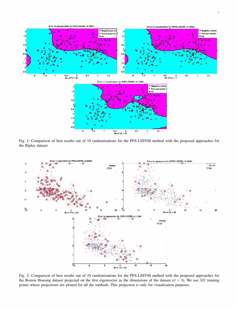
Table IV provides a comparison of the mean estimatederror, mean value of cardinality of prototype vectors (PV orSV, denoted in Table IV by SV) and a comparison of themean run time computations of the proposed approaches withKeerthi’s, Lopez method, PFS-LSSVM and SVM methods forvarious classification and PFS-LSSVM and SVR methods fordifferent regression datasets. Figure 3 represents the estimatederror, run time performance and variations in the number ofprototype vectors for Adult dataset (ADU). From Figure 3,we observe that Keerthi’s method result in best predictionerrors but requires the maximum computation time as well.The variations in the prediction errors by the proposed SPFS-LSSVM and SSD-LSSVM method are insignificant and theirestimated errors are comparable to that of the PFS-LSSVMmethod though they require a much smaller prototype vectorsset. An important observation was that the SSD-LSSVMmethod produces the maximum amount of sparsity and hasthe least computation time without significant trade-off in error
and thus making it highly suitable for very large scale datasets.The SSD-LSSVM method works well because the initial setof prototype vectors (PV) that it selects is only helping toconstruct a basis set where this basis set is maximizing thequadratic Renyi entropy criterion. We also observe that thenumber of reduced prototype vectors (SV) can vary a lot forL0-norm based methods as during each randomization westart with a different initialization and after performing theiterative sparsification procedure we end up in a different localminimum. This results in variations in the number of reducedsupport vectors (SV) for these methods.
D. Performance Analysis
In case of classification datasets, the proposed approachescalled SPFS-LSSVM and SSD-LSSVM work much better incomparison with SVM methods both in terms of sparsity andprediction errors as observed from Table IV. Their errors arecomparable to those of PFS-LSSVM and Keerthi’s methodand in the case of the Forest Cover dataset even better thanPFS-LSSVM method. The amount of sparsity introduced isquite high for the proposed approaches, which is consistentwith the fact that the L0-norm leads to highly sparse solutions.However, an observation shows that the number of prototypevectors is reduced to a maximum extent in most of the datasetsfor the SSD-LSSVM approach. The SPFS-LSSVM methodresults in best prediction error for Breast-Cancer(BC) datasetwhile the SSD-LSSVM method gives best results for thevery large scale FC dataset as highlighted in Table IV. Theamount of sparsity introduced varies for different datasets. Forexample, for the BC dataset the PFS-LSSVM method uses33.65%, Keerthi’s method uses 6.59%, SPFS-LSSVM andSSD-LSSVM method use 5.71% and 1.76% of the trainingdata respectively as SV without significant trade-off in errors.
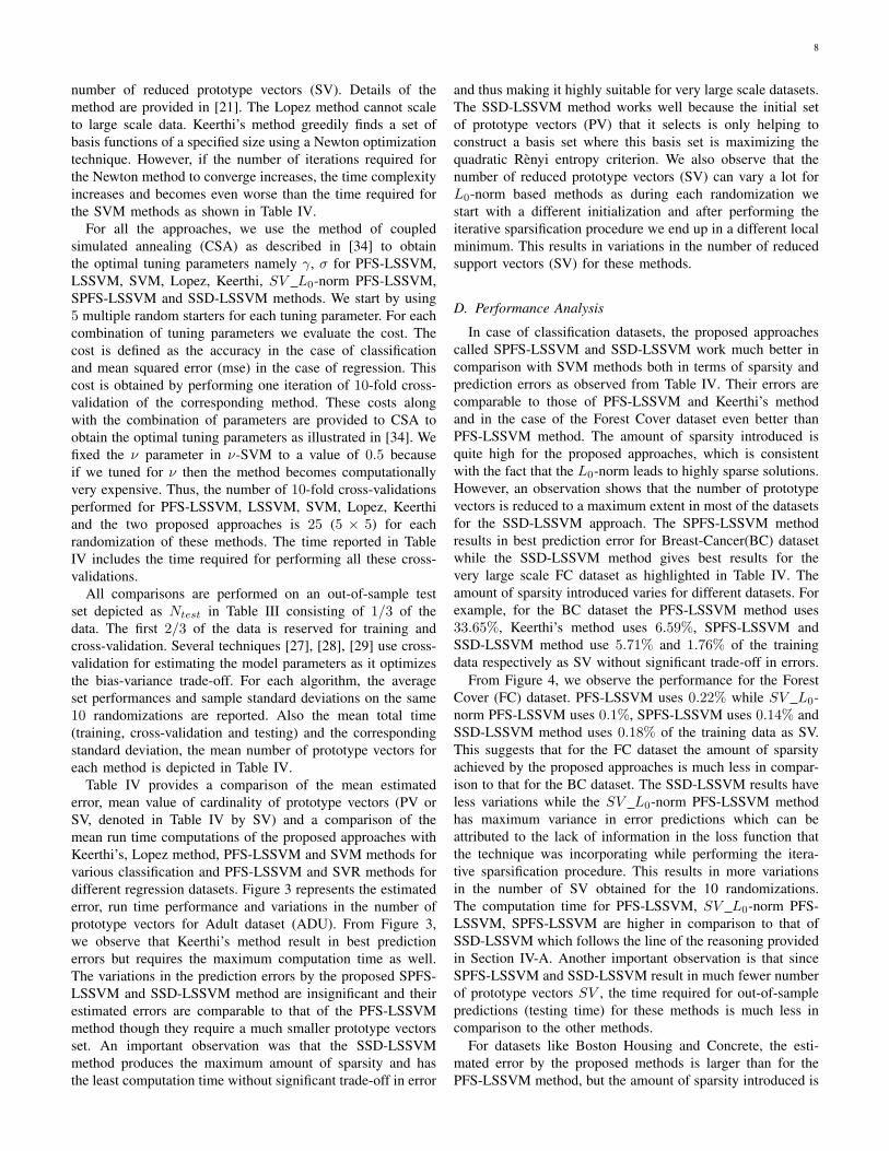
From Figure 4, we observe the performance for the ForestCover (FC) dataset. PFS-LSSVM uses 0.22% while SV L0-norm PFS-LSSVM uses 0.1%, SPFS-LSSVM uses 0.14% andSSD-LSSVM method uses 0.18% of the training data as SV.This suggests that for the FC dataset the amount of sparsityachieved by the proposed approaches is much less in compar-ison to that for the BC dataset. The SSD-LSSVM results haveless variations while the SV L0-norm PFS-LSSVM methodhas maximum variance in error predictions which can beattributed to the lack of information in the loss function thatthe technique was incorporating while performing the itera-tive sparsification procedure. This results in more variationsin the number of SV obtained for the 10 randomizations.The computation time for PFS-LSSVM, SV L0-norm PFS-LSSVM, SPFS-LSSVM are higher in comparison to that ofSSD-LSSVM which follows the line of the reasoning providedin Section IV-A. Another important observation is that sinceSPFS-LSSVM and SSD-LSSVM result in much fewer numberof prototype vectors SV , the time required for out-of-samplepredictions (testing time) for these methods is much less incomparison to the other methods.
For datasets like Boston Housing and Concrete, the esti-mated error by the proposed methods is larger than for thePFS-LSSVM method, but the amount of sparsity introduced is

9
Test
Cla
ssifi
catio
n(E
rror
and
Mea
nSV
)R
IPB
CD
IBSP
AM
MG
TA
DU
FCA
lgor
ithm
Err
orSV
Err
orSV
Err
orSV
Err
orSV
Err
orSV
Err
orSV
Err
orSV
PFS-
LSS
VM
[15]
0.10
2±
0.00
858
0.0
23±
0.0
04
153
0.21±
0.00
816
70.
08±
0.00
220
40.
134±
0.00
141
40.1
47±
0.0
664
0.2
048±
0.0
26
763
C-S
VC
[22]
0.1
5±
0.0
781
0.0
348±
0.0
241
40.3
32±
0.0
250
90.0
75±
0.0
67
800
0.1
44±
0.0
15
7000
0.1
51(∗
)11085(∗
)0.1
85(∗
)185000(∗
)ν
-SV
C[2
2]0.1
67±
0.0
311
20.0
28±
0.0
11
3980
.338±
0.0
17
512
0.1
13±
0.0
715
250.1
58±
0.0
14
7252
0.1
61(∗
)12205(∗
)184(∗
)165205(∗
)L
opez
[20]
0.1
83±
0.1
70.
04±
0.01
117
0.24
8±
0.03
410
0.07
26±
0.00
534
0-
--
--
-K
eert
hi[2
3]0.1
29±
0.0
33
260.
0463±
0.03
730
0.22
8±
0.03
553
0.07±
0.00
517
50.1
35±
0.0
02
260
0.14
5±
0.00
249
40.
2054
(*)
762(
*)S
VL
0-n
orm
[21]
0.1
651±
0.1
315
0.02
3±
0.01
270.
27±
0.05
390.1
27±
0.0
915
20.1
5±
0.0
09
750.1
49±
0.0
01
236
0.23
46±
0.02
535
2SP
FS-L
SSV
M0.1
47±
0.0
311
0.02
1±
0.01
260.
273±
0.04
80.0
82±
0.0
02
169
0.14
1±
0.00
416
30.1
48±
0.0
464
0.2
195±
0.0
350
5SS
D-L
SSV
M0.1
3±
0.0
211
0.02
56±
0.00
78
0.22
7±
0.02
60.0
836±
0.0
05
630.1
35±
0.0
280
0.1
488±
0.0
01
102
0.19
05±
0.00
963
5Te
stR
egre
ssio
n(E
rror
and
Mea
nSV
)B
osto
nH
ousi
ngC
oncr
ete
Slic
eL
ocal
izat
ion
Yea
rPr
edic
tion
Alg
orith
mE
rror
SVE
rror
SVE
rror
SVE
rror
SVPF
S-L
SSV
M[1
5]0.
133±
0.00
211
30.
112±
0.00
619
30.
0554±
0.0
694
0.40
2±
0.03
471
8ε-
SVR
[22]
0.16±
0.05
226
0.23±
0.02
670
0.10
2(*)
1301
2(*)
0.46
5(*)
1924
20(*
)ν
-SV
R[2
2]0.
16±
0.04
195
0.22±
0.02
330
0.09
2(*)
1252
40.
472(
*)17
5250
(*)
Lop
ez[2
0]0.
16±
0.05
650.
165±
0.07
215
--
--
SV
L0-n
orm
[21]
0.19
2±
0.01
538
0.26
5±
0.02
250.
156±
0.13
381
0.49
5±
0.03
422
SPFS
-LSS
VM
0.17
6±
0.03
500.
2383±
0.04
460.
058±
0.00
265
10.
44±
0.05
595
SSD
-LSS
VM
0.18
9±
0.02
243
0.16
45±
0.01
754
0.05
6±
0.0
577
0.42±
0.01
688
Trai
n,C
ross
-val
idat
ion
&Te
stC
lass
ifica
tion(
Com
puta
tion
Tim
e)A
lgor
ithm
RIP
BC
DIB
SPA
MM
GT
AD
UFC
PFS-
LSS
VM
[15]
3.16±
0.18
27.3
6±
1.33
36.1
4±
2.4
182±
731
42±
6116
523±
540
1185
00±
9294
C-S
VC
[22]
4.6±
0.83
14.7
6±
161±
7510
10±
5320
603±
396
1397
3(*)
5896
2(*)
ν-S
VC
[22]
5.67±
1114
.91±
183
.5±
115
785±
2213
901±
189
1399
2.7(
*)53
478(
*)L
opez
[20]
5.12±
0.9
28.2±
5.4
39.1±
5.9
950±
78.5
--
-K
eert
hi[2
3]21
.1±
0.6
74.3
4±
3.9
86.7±
5.12
1070±
37.7
1660
8±
397
2035
9±
762
9149
.8(*
)S
VL
0-n
orm
[21]
3.19±
0.16
27.3
84±
1.32
36.1
8±
2.4
182.
2±
731
43±
6116
527±
539
1185
40±
9267
.9SP
FS-L
SSV
M3.
21±
0.16
27.4
2±
1.33
36.2
66±
2.4
182.
3±
731
55±
6116
588±
529
1185
70±
9247
.6SS
D-L
SSV
M0.
955±
0.05
8.67±
0.14
11.8
2±
0.14
81.5±
0.6
2192±
1.9
1348
2±
15.6
8646
0±
2.8
Trai
n,C
ross
-val
idat
ion
&Te
stR
egre
ssio
n(C
ompu
tatio
nal
Tim
e)A
lgor
ithm
Bos
ton
Hou
sing
Con
cret
eSl
ice
Loc
aliz
atio
nY
ear
Pred
ictio
nPF
S-L
SSV
M[1
5]14
.28±
0.2
58.4
1±
1.41
3376
9±
1571
2480
46±
1533
0ε-
SVR
[22]
63±
116
8±
352
438(
*)67
231(
*)ν
-SV
R[2
2]61±
113
1±
242
724(
*)59
899(
*)L
opez
[20]
158.
6±
3.2
753±
35.5
--
SV
L0-n
orm
[21]
14.5
8±
0.2
58.6±
1.48
3377
5±
1574
2481
78±
1526
2SP
FS-L
SSV
M14
.5±
0.2
58.7
6±
1.44
3379
0±
1571
2484
12±
1524
8SS
D-L
SSV
M3.
75±
0.06
21.3
5±
0.13
725
991±
1186
652±
24
TAB
LE
IV:
Com
pari
son
inpe
rfor
man
ceof
the
diff
eren
tm
etho
dsfo
rU
CI
repo
sito
ryda
tase
ts.T
he(*
)re
pres
ents
nocr
oss-
valid
atio
nan
dpe
rfor
man
ceon
afix
edva
lue
oftu
ning
para
met
ers
due
toco
mpu
tatio
nal
burd
enan
d(-
)re
pres
ents
the
met
hod
cann
otsc
ale
for
this
data
set.
10
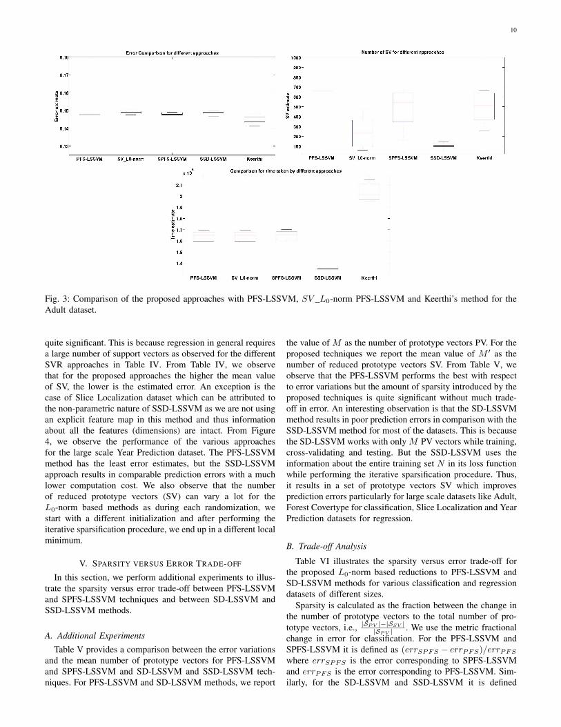
Fig. 3: Comparison of the proposed approaches with PFS-LSSVM, SV L0-norm PFS-LSSVM and Keerthi’s method for theAdult dataset.
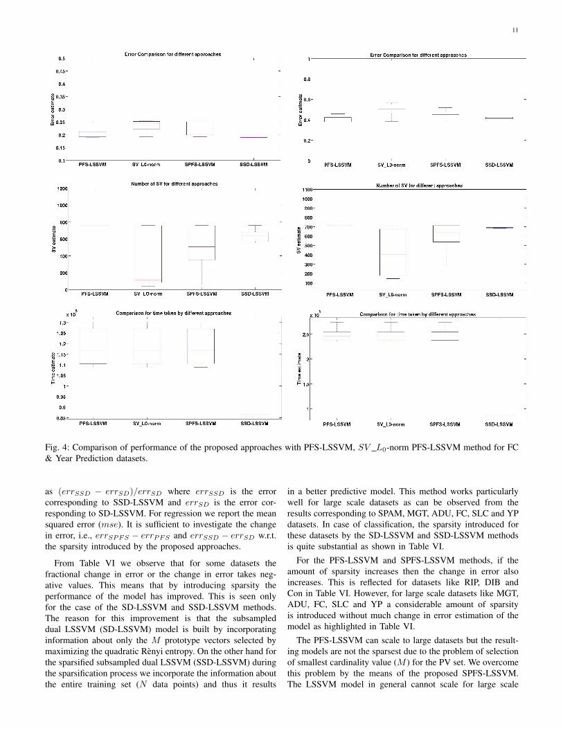
quite significant. This is because regression in general requiresa large number of support vectors as observed for the differentSVR approaches in Table IV. From Table IV, we observethat for the proposed approaches the higher the mean valueof SV, the lower is the estimated error. An exception is thecase of Slice Localization dataset which can be attributed tothe non-parametric nature of SSD-LSSVM as we are not usingan explicit feature map in this method and thus informationabout all the features (dimensions) are intact. From Figure4, we observe the performance of the various approachesfor the large scale Year Prediction dataset. The PFS-LSSVMmethod has the least error estimates, but the SSD-LSSVMapproach results in comparable prediction errors with a muchlower computation cost. We also observe that the numberof reduced prototype vectors (SV) can vary a lot for theL0-norm based methods as during each randomization, westart with a different initialization and after performing theiterative sparsification procedure, we end up in a different localminimum.
V. SPARSITY VERSUS ERROR TRADE-OFF
In this section, we perform additional experiments to illus-trate the sparsity versus error trade-off between PFS-LSSVMand SPFS-LSSVM techniques and between SD-LSSVM andSSD-LSSVM methods.
A. Additional Experiments
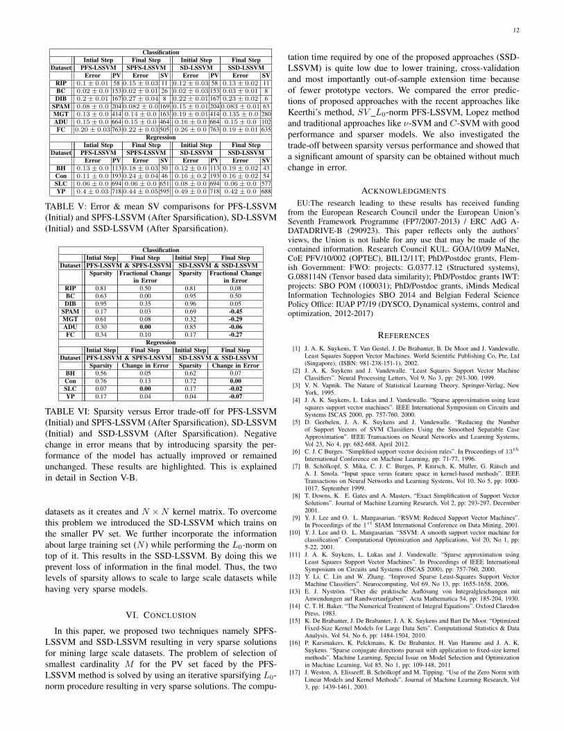
Table V provides a comparison between the error variationsand the mean number of prototype vectors for PFS-LSSVMand SPFS-LSSVM and SD-LSSVM and SSD-LSSVM tech-niques. For PFS-LSSVM and SD-LSSVM methods, we report
the value of M as the number of prototype vectors PV. For theproposed techniques we report the mean value of M ′ as thenumber of reduced prototype vectors SV. From Table V, weobserve that the PFS-LSSVM performs the best with respectto error variations but the amount of sparsity introduced by theproposed techniques is quite significant without much trade-off in error. An interesting observation is that the SD-LSSVMmethod results in poor prediction errors in comparison with theSSD-LSSVM method for most of the datasets. This is becausethe SD-LSSVM works with only M PV vectors while training,cross-validating and testing. But the SSD-LSSVM uses theinformation about the entire training set N in its loss functionwhile performing the iterative sparsification procedure. Thus,it results in a set of prototype vectors SV which improvesprediction errors particularly for large scale datasets like Adult,Forest Covertype for classification, Slice Localization and YearPrediction datasets for regression.
B. Trade-off Analysis
Table VI illustrates the sparsity versus error trade-off forthe proposed L0-norm based reductions to PFS-LSSVM andSD-LSSVM methods for various classification and regressiondatasets of different sizes.
Sparsity is calculated as the fraction between the change inthe number of prototype vectors to the total number of pro-totype vectors, i.e., |SP V |−|SSV |
|SP V | . We use the metric fractionalchange in error for classification. For the PFS-LSSVM andSPFS-LSSVM it is defined as (errSPFS − errPFS)/errPFS
where errSPFS is the error corresponding to SPFS-LSSVMand errPFS is the error corresponding to PFS-LSSVM. Sim-ilarly, for the SD-LSSVM and SSD-LSSVM it is defined
11
Fig. 4: Comparison of performance of the proposed approaches with PFS-LSSVM, SV L0-norm PFS-LSSVM method for FC& Year Prediction datasets.
as (errSSD − errSD)/errSD where errSSD is the errorcorresponding to SSD-LSSVM and errSD is the error cor-responding to SD-LSSVM. For regression we report the meansquared error (mse). It is sufficient to investigate the changein error, i.e., errSPFS − errPFS and errSSD − errSD w.r.t.the sparsity introduced by the proposed approaches.
From Table VI we observe that for some datasets thefractional change in error or the change in error takes neg-ative values. This means that by introducing sparsity theperformance of the model has improved. This is seen onlyfor the case of the SD-LSSVM and SSD-LSSVM methods.The reason for this improvement is that the subsampleddual LSSVM (SD-LSSVM) model is built by incorporatinginformation about only the M prototype vectors selected bymaximizing the quadratic Renyi entropy. On the other hand forthe sparsified subsampled dual LSSVM (SSD-LSSVM) duringthe sparsification process we incorporate the information aboutthe entire training set (N data points) and thus it results
in a better predictive model. This method works particularlywell for large scale datasets as can be observed from theresults corresponding to SPAM, MGT, ADU, FC, SLC and YPdatasets. In case of classification, the sparsity introduced forthese datasets by the SD-LSSVM and SSD-LSSVM methodsis quite substantial as shown in Table VI.
For the PFS-LSSVM and SPFS-LSSVM methods, if theamount of sparsity increases then the change in error alsoincreases. This is reflected for datasets like RIP, DIB andCon in Table VI. However, for large scale datasets like MGT,ADU, FC, SLC and YP a considerable amount of sparsityis introduced without much change in error estimation of themodel as highlighted in Table VI.
The PFS-LSSVM can scale to large datasets but the result-ing models are not the sparsest due to the problem of selectionof smallest cardinality value (M ) for the PV set. We overcomethis problem by the means of the proposed SPFS-LSSVM.The LSSVM model in general cannot scale for large scale
12
ClassificationIntial Step Final Step Initial Step Final Step
Dataset PFS-LSSVM SPFS-LSSVM SD-LSSVM SSD-LSSVMError PV Error SV Error PV Error SV
RIP 0.1± 0.01 58 0.15± 0.03 11 0.12± 0.03 58 0.13± 0.02 11BC 0.02± 0.0 153 0.02± 0.01 26 0.02± 0.03 153 0.03± 0.01 8DIB 0.2± 0.01 167 0.27± 0.04 8 0.22± 0.01 167 0.23± 0.02 6
SPAM 0.08± 0.0 204 0.082± 0.0 169 0.15± 0.01 204 0.083± 0.01 63MGT 0.13± 0.0 414 0.14± 0.0 163 0.19± 0.01 414 0.135± 0.0 280ADU 0.15± 0.0 664 0.15± 0.0 464 0.16± 0.0 664 0.15± 0.0 102FC 0.20± 0.03 763 0.22± 0.03 505 0.26± 0.0 763 0.19± 0.01 635
RegressionIntial Step Final Step Initial Step Final Step
Dataset PFS-LSSVM SPFS-LSSVM SD-LSSVM SSD-LSSVMError PV Error SV Error PV Error SV
BH 0.13± 0.0 113 0.18± 0.03 50 0.12± 0.0 113 0.19± 0.02 43Con 0.11± 0.0 193 0.24± 0.04 46 0.16± 0.2 193 0.16± 0.02 54SLC 0.06± 0.0 694 0.06± 0.0 651 0.08± 0.0 694 0.06± 0.0 577YP 0.4± 0.03 718 0.44± 0.05 595 0.49± 0.0 718 0.42± 0.0 688
TABLE V: Error & mean SV comparisons for PFS-LSSVM(Initial) and SPFS-LSSVM (After Sparsification), SD-LSSVM(Initial) and SSD-LSSVM (After Sparsification).
ClassificationIntial Step Final Step Initial Step Final Step
Dataset PFS-LSSVM & SPFS-LSSVM SD-LSSVM & SSD-LSSVMSparsity Fractional Change Sparsity Fractional Change
in Error in ErrorRIP 0.81 0.50 0.81 0.08BC 0.63 0.00 0.95 0.50DIB 0.95 0.35 0.96 0.05
SPAM 0.17 0.03 0.69 -0.45MGT 0.61 0.08 0.32 -0.29ADU 0.30 0.00 0.85 -0.06FC 0.34 0.10 0.17 -0.27
RegressionIntial Step Final Step Initial Step Final Step
Dataset PFS-LSSVM & SPFS-LSSVM SD-LSSVM & SSD-LSSVMSparsity Change in Error Sparsity Change in Error
BH 0.56 0.05 0.62 0.07Con 0.76 0.13 0.72 0.00SLC 0.07 0.00 0.17 -0.02YP 0.17 0.04 0.04 -0.07
TABLE VI: Sparsity versus Error trade-off for PFS-LSSVM(Initial) and SPFS-LSSVM (After Sparsification), SD-LSSVM(Initial) and SSD-LSSVM (After Sparsification). Negativechange in error means that by introducing sparsity the per-formance of the model has actually improved or remainedunchanged. These results are highlighted. This is explainedin detail in Section V-B.
datasets as it creates and N ×N kernel matrix. To overcomethis problem we introduced the SD-LSSVM which trains onthe smaller PV set. We further incorporate the informationabout large training set (N ) while performing the L0-norm ontop of it. This results in the SSD-LSSVM. By doing this weprevent loss of information in the final model. Thus, the twolevels of sparsity allows to scale to large scale datasets whilehaving very sparse models.
VI. CONCLUSION
In this paper, we proposed two techniques namely SPFS-LSSVM and SSD-LSSVM resulting in very sparse solutionsfor mining large scale datasets. The problem of selection ofsmallest cardinality M for the PV set faced by the PFS-LSSVM method is solved by using an iterative sparsifying L0-norm procedure resulting in very sparse solutions. The compu-
tation time required by one of the proposed approaches (SSD-LSSVM) is quite low due to lower training, cross-validationand most importantly out-of-sample extension time becauseof fewer prototype vectors. We compared the error predic-tions of proposed approaches with the recent approaches likeKeerthi’s method, SV L0-norm PFS-LSSVM, Lopez methodand traditional approaches like ν-SVM and C-SVM with goodperformance and sparser models. We also investigated thetrade-off between sparsity versus performance and showed thata significant amount of sparsity can be obtained without muchchange in error.
ACKNOWLEDGMENTS
EU:The research leading to these results has received fundingfrom the European Research Council under the European Union’sSeventh Framework Programme (FP7/2007-2013) / ERC AdG A-DATADRIVE-B (290923). This paper reflects only the authors’views, the Union is not liable for any use that may be made of thecontained information. Research Council KUL: GOA/10/09 MaNet,CoE PFV/10/002 (OPTEC), BIL12/11T; PhD/Postdoc grants, Flem-ish Government: FWO: projects: G.0377.12 (Structured systems),G.088114N (Tensor based data similarity); PhD/Postdoc grants IWT:projects: SBO POM (100031); PhD/Postdoc grants, iMinds MedicalInformation Technologies SBO 2014 and Belgian Federal SciencePolicy Office: IUAP P7/19 (DYSCO, Dynamical systems, control andoptimization, 2012-2017)
REFERENCES
[1] J. A. K. Suykens, T. Van Gestel, J. De Brabanter, B. De Moor and J. Vandewalle.Least Squares Support Vector Machines. World Scientific Publishing Co, Pte, Ltd(Singapore), (ISBN: 981-238-151-1), 2002.
[2] J. A. K. Suykens and J. Vandewalle. “Least Squares Support Vector MachineClassifiers”. Neural Processing Letters, Vol 9, No 3, pp: 293-300, 1999.
[3] V. N. Vapnik. The Nature of Statistical Learning Theory. Springer-Verlag, NewYork, 1995.
[4] J. A. K. Suykens, L. Lukas and J. Vandewalle. “Sparse approximation using leastsquares support vector machines”. IEEE International Symposium on Circuits andSystems ISCAS 2000, pp. 757-760, 2000.
[5] D. Geebelen, J. A. K. Suykens and J. Vandewalle. “Reducing the Numberof Support Vectors of SVM Classifiers Using the Smoothed Separable CaseApproximation”. IEEE Transactions on Neural Networks and Learning Systems,Vol 23, No 4, pp: 682-688, April 2012.
[6] C. J. C Burges. “Simplified support vector decision rules”. In Proceedings of 13th
International Conference on Machine Learning, pp: 71-77, 1996.[7] B. Scholkopf, S. Mika, C. J. C. Burges, P. Knirsch, K. Muller, G. Ratsch and
A. J. Smola. “Input space verus feature space in kernel-based methods”. IEEETransactions on Neural Networks and Learning Systems, Vol 10, No 5, pp: 1000-1017, September 1999.
[8] T. Downs, K. E. Gates and A. Masters. “Exact Simplification of Support VectorSolutions”. Journal of Machine Learning Research, Vol 2, pp: 293-297, December2001.
[9] Y. J. Lee and O. L. Mangasarian. “RSVM: Reduced Support Vector Machines”.In Proceedings of the 1st SIAM International Conference on Data Mining, 2001.
[10] Y. J. Lee and O. L. Mangasarian. “SSVM: A smooth support vector machine forclassification”. Computational Optimization and Applications, Vol 20, No 1, pp:5-22, 2001.
[11] J. A. K. Suykens, L. Lukas and J. Vandewalle. “Sparse approximation usingLeast Squares Support Vector Machines”. In Proceedings of IEEE InternationalSymposium on Circuits and Systems (ISCAS 2000), pp: 757-760, 2000.
[12] Y. Li, C. Lin and W. Zhang. “Improved Sparse Least-Squares Support VectorMachine Classifiers”. Neurocomputing, Vol 69, No 13, pp: 1655-1658, 2006.
[13] E. J. Nystrom. “Uber die praktische Auflosung von Integralgleichungen mitAnwendungen auf Randwertaufgaben”. Acta Mathematica 54, pp: 185-204, 1930.
[14] C. T. H. Baker. “The Numerical Treatment of Integral Equations”. Oxford ClaredonPress, 1983.
[15] K. De Brabanter, J. De Brabanter, J. A. K. Suykens and Bart De Moor. “OptimizedFixed-Size Kernel Models for Large Data Sets”. Computational Statistics & DataAnalysis, Vol 54, No 6, pp: 1484-1504, 2010.
[16] P. Karsmakers, K. Pelckmans, K. De Brabanter, H. Van Hamme and J. A. K.Suykens. “Sparse conjugate directions pursuit with application to fixed-size kernelmethods”. Machine Learning, Special Issue on Model Selection and Optimizationin Machine Learning, Vol 85, No 1, pp: 109-148, 2011
[17] J. Weston, A. Elisseeff, B. Scholkopf and M. Tipping. “Use of the Zero Norm withLinear Models and Kernel Methods”. Journal of Machine Learning Research, Vol3, pp: 1439-1461, 2003.
13
[18] E. J. Candes, M. B. Wakin and S. Boyd. “Enhancing Sparsity by Reweighted l1Minimization”. Journal of Fourier Analysis and Applications, Vol 14, No 5, pp:877-905, special issue on sparsity, 2008.
[13] G. C. Cawley and N. L. C. Talbot. “Improved sparse least-squares support vectormachines”. Neurocomputing, Vol 48, No 1-4, pp: 1025-1031, 2002.
[19] K. Huang, D. Zheng, J. Sun, Y. Hotta, K. Fujimoto and S. Naoi. “Sparse Learningfor Support Vector Classification”. Pattern Recognition Letters, Vol 31, No 13, pp:1944-1951, 2010.
[20] J. Lopez, K. De Brabanter, J. R. Dorronsoro and J. A. K. Suykens. “SparseLSSVMs with L0-norm minimization”. In Proceedings of the European Sym-posium on Artificial Neural Networks, Computational Intelligence and MachineLearning (ESANN 2011), pp: 189-194, Belgium, 2011.
[21] R. Mall and J. A. K. Suykens. “Sparse Variations to Fixed-Size Least SquaresSupport Vector Machines for Large Scale Data”. In the The 17th Pacific-AsiaConference on Knowledge Discovery and Data Mining (PAKDD2013). ftp://ftp.esat.kuleuven.be/SISTA/rmall/PAKDD ms.pdf
[22] C. C. Chang and C. J. Lin. “LIBSVM : a library for support vector machines”,ACM Transactions on Intelligent Systems and Technology, Vol 2, No 27, pp.1-27,2011.
[23] S. S. Keerthi, O. Chapelle and D. DeCoste. “Building support vector machineswith reduced classifier complexity”. Journal of Machine Learning Research, Vol7, pp: 1493-1515, July 2006.
[24] C. L. Blake and C. J. Merz. “UCI repository of machine learning databases”.http://archive.ics.uci.edu/ml/datasets.html , Irvine, CA.
[25] R. Fletcher. Practical methods of Optimization. John Wiley & Sons, 1987.[26] C. K. I. Williams and M. Seeger. “Using the Nystrom method to speed up kernel
machines”. Advances in Neural Information Processing Systems, Vol 13, pp: 682-688, 2001.
[27] M. Rudemo. “Empirical choice of histograms and kernel density estimators”.Scandinavian Journal of Statistics, Vol 9, pp: 65-78, 1982.
[28] L. Du, Y. Yang, D. He, R. G. Harley, T. G. Habetler and B. Lu. “SupportVector Machines Based Methods For Non-Intrusive Identification of MiscellaneousElectric Loads”, 38th Annual Conference of the IEEE Industrial ElectronicsSociety (IECON 2012), October 25-28, Montreal, Quebec, Canada.
[29] A. W. Bowman. “An alternative method of cross-validation for smoothing ofdensity estimators”. Biometrika, Vol 71, pp: 353-360, 1984.
[30] D. W. Scott and G. R. Terrel. “Biased and unbiased cross-validation in densityestimation”. Journal of American Statistical Association, Vol 82, pp: 1131-1146,1987.
[31] C. C. Taylor. “Bootstrap choice of the smoothing parameter in kernel densityestimation”. Biometrika, Vol 76, pp: 705-712, 1989.
[32] S. J. Sheather and M. C. Jones. “A reliable data-based bandwidth selection methodfor kernel density estimation”. Journal of the Royal Statistical Society, Vol 53, pp:683-690, 1991.
[33] D. W. Scott and S. R. Sain. “Multi-dimensional Density Estimation”. Data Miningand Computational Statistics, Vol 23, pp: 229-263, 2004.
[34] S. Xavier de Souza, J. A. K. Suykens, J. Vandewalle and D. Bolle. “CoupledSimulated Annealing for Continuous Global Optimization”. IEEE Transactions onSystems, Man, and Cybertics - Part B, Vol 40, No 2, pp: 320-335, 2010.
Johan A.K. Suykens received the degree in Electro-Mechanical Engineering and the Ph.D. degree inApplied Sciences from the KU Leuven, in 1989and 1995, respectively. In 1996 he has been aVisiting Postdoctoral Researcher at the Universityof California, Berkeley. He has been a PostdoctoralResearcher with the Fund for Scientific ResearchFWO Flanders and is currently a Professor with KULeuven. He is author of the books ”Artificial NeuralNetworks for Modelling and Control of Non-linearSystems” (Kluwer Academic Publishers) and ”Least
Squares Support Vector Machines” (World Scientific), co-author of the book”Cellular Neural Networks, Multi-Scroll Chaos and Synchronization” (WorldScientific) and editor of the books ”Nonlinear Modeling: Advanced Black-BoxTechniques” (Kluwer Academic Publishers), ”Advances in Learning Theory:Methods, Models and Applications” (IOS Press) and Regularization, Opti-mization, Kernels, and Support Vector Machines (Chapman and Hall/CRC).He is a Senior IEEE member and has served as associate editor for the IEEETransactions on Circuits and Systems (1997-1999 and 2004-2007) and for theIEEE Transactions on Neural Networks (1998-2009). He received an IEEESignal Processing Society 1999 Best Paper Award and several Best PaperAwards at International Conferences. He is a recipient of the InternationalNeural Networks Society INNS 2000 Young Investigator Award for significantcontributions in the field of neural networks. He has been awarded an ERCAdvanced Grant 2011.
Raghvendra Mall was born in Kolkata, India onMarch 5th, 1988. He received his BTech degree in2010 and MS by Research in Computer Science in2011 from IIIT-Hyderabad, India. He is started hisdoctorate at ESAT-STADIUS, KU Leuven, Leuven,Belgium in 2012 under the guidance of Prof. JohanA.K. Suykens. He is currently developing techniquesto explore sparsity in large scale machine learn-ing problems. His current research interests includesampling and community detection in complex net-works,exploring the role of sparsity in classification,
clustering and regression.